$R$-current six-point correlators in $AdS_{5}$ Supergravity

Abstract

Within the conjectured duality between ${\cal N}=4$ super Yang-Mills and Anti-deSitter string theory, the BFKL Pomeron of the gauge theory corresponds to the graviton mode of the dual string. As a first step towards analyzing multigraviton exchange, we investigate $R$-current six-point functions within the supergravity approximation. We compute the analogue of diffractive scattering, and we analyze the triple Regge limit. In the supergravity approximation the triple graviton vertex is found to vanish.

DESY–09–217

1 Introduction

Since many years, the high energy behavior of scattering amplitudes in quantum field theory has attracted interest, and extensive calculations have been performed in order to understand the structure well beyond leading orders of perturbation theory. In this context, a special role is played by the Regge limit which is closely connected with unitarity of the theory.

The AdS/CFT correspondence [1, 2, 3, 4] has raised new hopes to determine the high energy behavior to all orders of the ’t Hooft coupling $\lambda$, including the strong coupling region, at least for those gauge theories which possess a dual string theory description. The most prominent example of such a duality relates 4D super Yang-Mills (SYM) theory with ${\cal N}=4$ supersymmetries to type IIB string theory in the Anti-deSitter background $AdS_{5}\times S_{5}$. Through the correspondence, the gauge theoretic BFKL Pomeron [5, 6, 7] gets related to graviton on the string theory side [8, 9].

In [10] and [11] we have examined this correspondence in some detail. Stimulated by QCD where $\gamma^{*}\gamma^{*}$ scattering provides a safe framework for investigating the BFKL Pomeron, we have studied the elastic scattering of two $R$-currents [12] in ${\cal N}=4$ SYM theory. On the weak coupling side, the high energy scattering amplitude factorizes into the current impact factors and the BFKL Green’s function. In [10] the $R$-current impact factor has been calculated to leading order. The BFKL Green’s function is known also in NLO [13, 14, 15]. In the strong coupling region, the method of calculating leading order correlations function was defined in [3]. It involves the summation of Witten diagrams containing supergravity fields which live on the $AdS_{5}$ space. Our calculation of the high energy behavior of Witten diagrams has shown that the scattering amplitudes for infinite ’t Hooft coupling $\lambda$ also come as a convolution of impact factors and an exchange propagator, just as in the weakly coupled theory. The convolution is defined through an integration over the radial direction of the $AdS_{5}$ geometry. As a result of our calculation, we have obtained an expression for the $R$-current impact factor at $\lambda\to\infty$. Corrections of the order $1/\lambda$ require string theory calculations. As to the exchanged graviton, Witten diagrams in the Regge limit yield a power law behavior ${\cal A}_{graviton}\sim s^{j}$, with $j=2$ being the spin of the graviton. The higher order corrections to the graviton trajectory

$$j\ =\ 2-\frac{4+\nu^{2}}{2\sqrt{\lambda}}+{\cal O}(\frac{1}{\lambda})\,,$$ (1.1)

cannot be derived from Witten diagrams, and they have been deduced from other lines of arguments [8, 9]. In [16] a representation for the Regge limit of four current correlators has been suggested which would allow to interpolate between weak and strong limits. We have not attempted to cast our result for the Witten diagram into this form.

Within QCD, it is well known that the BFKL Pomeron violates unitarity bounds since it grows as ${\cal A}_{BFKL}\sim is^{j}$ with $j=1+\omega_{BFKL}$ at very high energies. Consequently the Pomeron must be tamed by suitable corrections. Elaborate calculations have been performed in order to identify the relevant corrections within perturbation theory. An example arises in the context of deep inelastic electron proton scattering at small $x$ (which is related to the elastic scattering of a virtual photon on the proton). It has been argued that the most important corrections to the BFKL exchange are given by ’fan’ diagrams (an example is shown in fig. 1a) which contain the triple Pomeron vertex. This vertex describes the splitting of one BFKL Pomeron into two Pomerons. A derivation of this result is obtained by considering, first, the scattering of the virtual photon on two (weakly coupled) nucleons and, then, closing the two BFKL Pomerons at the lower end by integrating over the ’diffractive’ squared mass $M^{2}$ (fig. 1b). As a key feature, the fan diagram in fig. 1a. contains, in its lower part, the exchange of two BFKL Pomerons which comes with a minus sign relative to the single BFKL exchange. At high energies, double Pomeron exchange grows as ${\cal A}_{double\,\,BFKL}\sim-is^{1+2\omega_{BFKL}}$, and thus starts to weaken the growth of the single BFKL exchange. In preparation for extending this discussion to ${\cal N}=4$ SYM theory, one may replace the two nucleons at the bottom by virtual photons. In this way, the essential amplitude to be studied, becomes the six-point electromagnetic current correlator, evaluated in the triple Regge limit. It is a remarkable feature of QCD that the two lower Pomerons do not couple directly to the upper impact factor. Such a ’direct’ coupling would correspond to the eikonal approximation. The absence of this direct coupling in the leading logarithmic approximation of QCD means that the eikonal picture is not supported.

Turning to ${\cal N}=4$ SYM theory, the analogous correlator is the six-point correlator of $R$-currents. Our comments on QCD suggest to investigate, as a first step of addressing the unitarization, the six-point $R$-current correlator in the limit $s_{1}\sim s_{2}\gg M^{2}$.

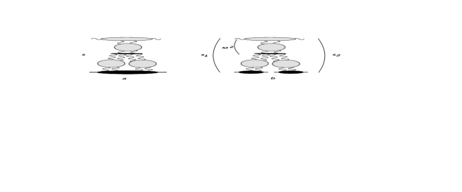
Figure 1: Unitarity corrections in QCD: (a) a fan diagram; (b) the six-point function

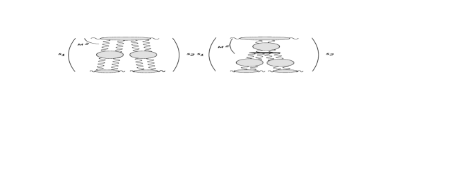
Figure 2: High energy limit of the six-point function in ${\cal N}=4$ SYM

In the weak coupling limit, this high energy limit of the six-point $R$-current correlator in ${\cal N}=4$ SYM theory has been studied in [17]. The main result is illustrated in fig. 2. At high energies, the six-point amplitude can be written as a sum of several pieces [18]; each of them corresponds to a distinct set of simultaneous energy discontinuities, in agreement with the Steinmann relations. For our discussion we are interested only in those terms which contribute to the discontinuity in the energies $s_{1}$, $s_{2}$ and in the square of the diffractive mass, $M^{2}$. In the leading log approximation, the triple Pomeron vertex (fig. 2, right figure) is the same as in QCD. The amplitude corresponding to this diagram has the form

$${\cal A}_{3\to 3}^{triple}\ =\ \frac{s_{1}s_{2}}{M^{2}}\int\int\int\frac{d\omega d\omega_{1}d\omega_{2}}{(2\pi i)^{3}}s_{1}^{\omega_{1}}s_{2}^{\omega_{2}}(M^{2})^{\omega-\omega_{1}-\omega_{2}}\\ \xi(\omega_{1})\xi(\omega_{2})\xi(\omega,\omega_{1},\omega_{2})F(\omega,\omega_{1},\omega_{2})\,,$$

where the signature factors are given by

$$\xi(\omega)\ =\ -\pi\frac{e^{-ipi\omega}-1}{\sin\pi\omega}\quad,\quad\,\,\,\xi(\omega,\omega_{1},\omega_{2})\ =\ -\pi\frac{e^{-i\pi(\omega-\omega_{1}-\omega_{2})}-1}{\sin\pi(\omega-\omega_{1}-\omega_{2})}\,,$$ (1.2)

and

$$F(\omega,\omega_{1},\omega_{2})\ =\ \Phi(Q^{2})\otimes G(\omega)\otimes V\otimes G(\omega_{1})\otimes\Phi(Q_{A}^{2})\otimes G(\omega_{2})\otimes\Phi(Q_{B}^{2})\,.$$ (1.3)

Here $\otimes$ denotes the integration over transverse momenta, $G(\omega)$ is the BFKL Green’s function, $\Phi$ is the impact factor presented in  [10], and details on the triple Pomeron vertex $V$ can be can be found in [17]. The discontinuity of this six-point function across the cut in $M^{2}$ leads to the cross section of the diffractive scattering process (in the notations of QCD) $\gamma^{*}+\gamma^{*}\to M_{X}+\gamma^{*}$. Since $M^{2}$ is large, we obtain a contribution of ’large diffractive masses’. In all three $\omega$ variables, the leading singularity is given by the BFKL characteristic functions

$$\omega\ =\ \omega_{1}\ =\ \omega_{2}\ =\ \alpha_{s}\chi(\nu=0,n=0)\ =\ \frac{4N_{c}\alpha_{s}\ln 2}{\pi}\ .$$ (1.4)

As an important feature of ${\cal N}=4$ SYM theory we find an extra contribution (see fig. 2, left figure) where the two BFKL exchanges couple directly to the upper $R$-currents. The presence of this ’direct’ coupling, which is absent in QCD and might be viewed as a support of eikonalization in ${\cal N}=4$ SYM theory, can be traced back to the fact that fermions (and scalars) belong to the adjoint representation. The corresponding scattering amplitude is of the form

$${\cal A}_{3\to 3}^{direct}\ =\ s_{1}s_{2}\int\int\frac{d\omega_{1}d\omega_{2}}{(2\pi i)^{2}}s_{1}^{\omega_{1}}s_{2}^{\omega_{2}}\xi(\omega_{1})\xi(\omega_{2})F(M^{2};\omega_{1},\omega_{2})\,,$$ (1.5)

where

$$F(M^{2};\omega_{1},\omega_{2})\ =\ \Phi(Q^{2};M^{2})^{direct}\otimes G(\omega_{1})\otimes\Phi(Q_{A}^{2})\otimes G(\omega_{2})\otimes\Phi(Q_{B}^{2})\,.$$ (1.6)

An expression for the new impact factor $\Phi(M^{2};Q^{2}))^{direct}$ which describes the coupling of the two BFKL Pomerons to the upper $R$-current can be found in [19, 20] and [17, 21] . For large $M^{2}$, this impact factor falls off as $M^{-4}$. For the diffractive cross section one takes the $M^{2}$-discontinuity of the six-point amplitude, i.e. the $M^{2}$-discontinuity of the impact factor $\Phi(M^{2};Q^{2}))^{direct}$. The latter falls off as $M^{-8}$, i.e. it contributes to the region of small diffractive masses.

In the present paper we continue the investigtion of the high energy limit in the strongly coupled theory using Witten diagrams. Our main interest now is in the six-point $R$-current correlators. In the triple Regge limit, the amplitude is dominated by $t-$channel exchanges of gravitons. The relevant diagrams are shown in figs. 3 and 4. There is an obvious correspondence between the two contributions on the weak (fig. 2) and on the strong coupling side (figs. 3 and 4, left diagram).

Figure 3: Witten diagrams for the two graviton exchange in the $t-$channel

These Witten diagrams will be considered as the strong coupling analogue of our weak coupling results obtained in ${\cal N}=4$ SYM theory .

Our article is organized as follows. Section 2 is devoted to a brief review of our notation used in [11]. In section 3 we present computations of the scattering amplitude with the two $t-$channel gravitons and one intermediate $R$-boson carrying mass $M$ (fig. 3). We rewrite the amplitude to momentum space and perform the high energy limit. The amplitude is found to be proportional to the square of two large energy variables, namely $s_{1}^{2}s_{2}^{2}$. The planar graph (left part of fig. 3) has a cut for positive $M^{2}$, starting at $M^{2}=0$, and, for large $M^{2}$ (triple Regge limit), falls off as $M^{-2}$. Correspondingly, the crossed graph (right part of fig. 3) has a cut for negative values of $M^{2}$. Finally, in section 4 we consider the correlation function with the triple graviton vertex (fig. 4). In the triple Regge limit, the expected contribution to the triple Regge behavior $\sim(s_{1}/M^{2})^{j_{1}}(s_{2}/M^{2})^{j_{2}}(M^{2})^{j}$ with $j=j_{1}=j_{2}=2$ vanishes. Instead, we find contributions proportional to $s_{1}^{2}$, $s_{2}^{2}$, and $s_{1}s_{2}$.

Figure 4: Left figure: triple graviton exchange with the triple graviton vertex. Right figure: two graviton exchange with the direct coupling of two gravitons and two bosons.

2 Six-point correlation functions at strong coupling

Let us consider ${\cal N}=4$ super Yang-Mills (SYM) theory in four dimensional Euclidean space. The Fourier transform of the six-point correlator reads as

$$(2\pi)^{4}\delta(\sum_{i=1}^{6}\vec{p}_{i})A_{j_{1}j_{2}j_{3}j_{4}j_{5}j_{6}}(\vec{p}_{i})\ =\ \int\left(\prod_{i=1}^{6}d^{4}x_{i}\mathop{\rm e}\nolimits^{-i\vec{p}_{i}\cdot\vec{x}_{i}}\right)\langle\prod_{a=1}^{6}J_{j_{a}}(\vec{x}_{a})\rangle\,.$$ (2.1)

By $J_{j}$ we denote $R$-currents with $j$ labelling the spacial directions, $j=1,\dots,d=4$. The $\vec{x}=(x_{1},x_{2},x_{3},x_{4})$ stands for the four dimensional Euclidean vector (the value $j=0$ refers to the fifth coordinate).

We use the same notations as in  [11]. Starting with the Euclidean notation $\vec{p}=(p_{1},p_{2},p_{3},p_{4})$ and $|\vec{p}|=\sqrt{\vec{p}^{2}}$, the Wick rotation continues $|\vec{p}|^{2}=\vec{p}^{2}\to-p^{2}=-p_{4}^{2}+p_{1}^{2}+p_{2}^{2}+p_{3}^{2}$ in Minkowski space. In the high energy limit, our scattering amplitude depends upon the energies $s_{1}$, $s_{2}$, the diffractive mass squared $M^{2}$, and the momentum transfers $t_{1}$, $t_{2}$, and $t$. Furthermore, $|\vec{p}_{1}|$, $|\vec{p}_{2}|$, $|\vec{p}_{3}|$, ($|\vec{p}_{4}|$ ,$|\vec{p}_{5}|$ and $|\vec{p}_{6}|$) are the virtualities of the incoming (outgoing) currents. In Euclidean notation we have

$$s_{1}\ =\ -(\vec{p}_{1}+\vec{p}_{2})^{2}\,,\quad s_{2}\ =\ -(\vec{p}_{1}+\vec{p}_{3})^{2}\,,\quad M^{2}\ =\ -(\vec{p}_{1}+\vec{p}_{2}+\vec{p}_{5})^{2}\,,\quad$$

$$-t\ =\ (\vec{p}_{1}+\vec{p}_{4})^{2}\,,\quad-t_{1}\ =\ (\vec{p}_{2}+\vec{p}_{5})^{2}\,,\quad-t_{2}\ =\ (\vec{p}_{3}+\vec{p}_{6})^{2}\,.\quad$$ (2.2)

After Wick rotations, the energy variables $s_{1}$, $s_{2}$, and $M^{2}$ are positive, whereas the momentum transfer variables $t$, $t_{1}$, $t_{2}$ remain negative; the masses of the external currents are kept negative (space-like), $-|\vec{p}_{i}|$. After Wick rotation, we still continue to use the vector symbol $\vec{p}$ for the Minkowski vector $(p_{1},p_{2},p_{3},p_{4})$, but now $\vec{p}^{2}=-p^{2}$.

The high energy limit is defined as

$$s_{1},\,s_{2}\,\gg M^{2}\,-t,\,-t_{1},\,-t_{2},-|\vec{p}_{i}|^{2}.$$ (2.3)

For the two graviton exchange diagrams we will keep $M^{2}$ finite, whereas for the triple graviton diagram we take the triple Regge limit where also $M^{2}$ becomes large.

Finally, we find it convenient to present the scattering amplitude in the helicity basis. To this end we contract the correlator $A$ with appropriate polarization vectors

$${\cal A}_{\lambda_{1}\lambda_{2}\lambda_{3};\lambda_{4}\lambda_{5}\lambda_{6}}(|\vec{p}_{i}|;s_{1},s_{2},M^{2};t,t_{1},t_{2})\ =$$

$$\hskip 5.69054pt=\sum_{j_{i}}\epsilon_{j_{1}}^{(\lambda_{1})}(\vec{p}_{1})\epsilon_{j_{2}}^{(\lambda_{2})}(\vec{p}_{2})\epsilon_{j_{3}}^{(\lambda_{3})}(\vec{p}_{3})\epsilon_{j_{4}}^{(\lambda_{4})}(\vec{p}_{4})^{\ast}\epsilon_{j_{5}}^{(\lambda_{5})}(\vec{p}_{5})^{\ast}\epsilon_{j_{6}}^{(\lambda_{6})}(\vec{p}_{6})^{\ast}{A}_{j_{1}j_{2}j_{3}j_{4}j_{5}j_{6}}(\vec{p}_{i})\,,$$ (2.4)

where $\lambda_{i}=L,\pm$ runs through the possible helicities and we introduced the polarization vectors $\epsilon_{j}^{\lambda_{i}}(\vec{p}_{i})$ such that $p_{i}^{j}\epsilon_{j}^{(\lambda_{i})}(\vec{p_{i}})=0$.

In order to calculate the amplitude (2.1) in the limit of infinite ’t Hooft coupling [10] we make use of the conjectured AdS/CFT correspondence [2] between IIB string theory on $AdS_{5}$ space and ${\cal N}=4$ $SU(N_{c})$ super Yang-Mills theory. An efficient calculation can only be performed in the limit of large $N_{c}$. Moreover the full string theory on $AdS_{5}$ is well approximated by classical supergravity when ’t Hooft coupling $\lambda=g^{2}_{YM}N_{c}$ goes to infinity.

According to the AdS/CFT correspondence, correlation functions are related with a classical supergravity action $S_{AdS}$ by  [3, 4]

$$\langle J(1)J(2)\ldots J(n)\rangle_{CFT}\ =\ \omega_{n}\frac{\delta^{n}}{\delta\phi_{0}(1)\ldots\delta\phi_{0}(n)}\exp(-S_{AdS}[\phi[\phi_{0}]])\big{|}_{\phi_{0}=0}\,,$$ (2.5)

where the factor $\omega_{n}$ comes from the relative normalization [22] while the sources $\phi_{0}$ of operators in super Yang-Mills theory correspond to the boundary values of supergravity fields in $AdS_{5}$ in the $4$-dimensional quantum field theory, i.e. $\phi|_{\partial AdS}\sim\phi_{0}$. We are using the following conventions concerning the Anti-deSitter space $AdS_{d+1}$. Its Euclidean continuation is parameterized by $z_{0}>0$ and $\vec{x}$ with coordinates $x_{i}$ enumerated by the Latin indices $i=1,\ldots,d$. We use the metric

$$ds^{2}\ =\ \frac{1}{z_{0}^{2}}(dz_{0}^{2}+d\vec{x}^{2})\,,$$ (2.6)

where $d\vec{x}^{2}$ can be related to the metric of Minkowski space by Wick rotation. The limit $z_{0}\to 0$ corresponds to the boundary of the Anti-deSitter space. The most interesting case is for $d=4$ which can be related to QCD.

To simplify notation we truncate the $SU(4)$ $R$-current group to $U(1)_{R}$. However, our considerations may easily be generalized to the non-Abelian case. The supergravity action is defined by

$$S\ =\ \frac{1}{2\kappa_{d+1}^{2}}\int d^{d+1}z\sqrt{g}(-{\cal R}+\Lambda)+S_{m}\,,$$ (2.7)

where ${\cal R}$ is the scalar curvature while the covariant matter action reads as [23, 22, 24, 25]

$$S_{m}\ =\ \frac{1}{2\kappa_{d+1}^{2}}\int d^{d+1}z\sqrt{g}\left[\frac{1}{4}F_{\mu\nu}F^{\mu\nu}-A_{\mu}J^{\mu}+\ldots\right]\ .$$ (2.8)

Here $\kappa_{5}^{2}$ is fixed by matching two- and three-point protected operators [23, 22], while $F_{\mu\nu}$ is the field strength of the gauge field $A$. Throughout this note, Greek indices refer to the $(d+1)$-dimensional space, i.e. they take values from $0$ to $d$. Latin subscripts, on the other hand, parameterize directions along the Euclidean $d$-dimensional boundary of $AdS_{d+1}$. Contractions of the full metric (2.6) are denoted with upper and lower indices while contractions of both lower indices denotes simple summation with Kronecker delta.

After these technical preparations we can now begin to evaluate the high energy limit of our six-point correlator at strong coupling, where supergravity on AdS is believed to provide an accurate description. To this end we make use of a very convenient and intuitive diagrammatic procedure that was first proposed by Witten [3] and then developed further by many other authors. It relies on summing diagrams which in our case contain only three basic building blocks, namely the bulk-to-bulk propagators for the graviton and the gauge $R$-bosons as well as the bulk-to-boundary $R$-boson propagator. They are connected by vertices defined in eqs. (2.7) and (2.8). In the high energy limit it is enough to analyze diagrams plotted in figs. 3, 4.

3 Two Graviton exchange: Low diffractive masses

In this section we analyze two Witten diagrams depicted in fig. 3. These will later turn out to contain all leading order contributions to the high energy limit of the full amplitude. After a very detailed discussion of the first diagram we can obtain the contribution from the second diagram through analytic continuation. The results are spelled out in eqs. (3.27) and (3.30). They involve a new impact factor, defined in eq. (3.21), whose properties shall be analyzed in subsection 3.3. The final subsection is then devoted to a study of the deep inelastic limit of the amplitude.

3.1 The Momentum space representation

We start from the expression for the two graviton exchange in configuration space. Its contribution to the six current matrix element is

$$I^{\rm 2G,planar} = \int\frac{d^{d+1}y}{y_{0}^{d-3}}\int\frac{d^{d+1}v}{v_{0}^{d-3}}\int\frac{d^{d+1}w}{w_{0}^{d-3}}\int\frac{d^{d+1}z}{z_{0}^{d-3}}\tilde{T}_{(14)\mu\nu,\rho\sigma}(z,y)$$

$$G_{\mu\nu;\mu^{\prime}\nu^{\prime}}(z,w)G_{\rho\sigma;\rho^{\prime}\sigma^{\prime}}(y,v)\tilde{T}_{(25)\mu^{\prime}\nu^{\prime}}(w)\tilde{T}_{(36)\rho^{\prime}\sigma^{\prime}}(v)\,,$$

where the stress-energy tensor

$$\tilde{T}_{(14)\mu\nu} = z_{0}^{2}\partial_{[\mu}G_{\lambda]\rho_{1}}(z,\vec{x}_{1})\partial_{[\nu}G_{\lambda]j_{4}}(z,\vec{x}_{4})+z_{0}^{2}\partial_{[\nu}G_{\lambda]\rho_{1}}(z,\vec{x}_{1})\partial_{[\mu}G_{\lambda]j_{4}}(z,\vec{x}_{4})$$ (3.2)

$$\hskip 56.9055pt-\frac{1}{2}z_{0}^{2}\delta_{\mu\nu}\partial_{[\alpha}G_{\beta]\rho_{1}}(z,\vec{x}_{1})\partial_{[\alpha}G_{\beta]j_{4}}(z,\vec{x}_{4})\,.$$

In the high energy limit, the highest contribution comes from the first two terms. For the coupling of the two gravitons to the upper currents one can define the double stress-energy tensor

$$\tilde{T}_{(14)\mu\nu,\rho\sigma} = (\delta_{\mu\mu^{\prime}}\delta_{\nu\nu^{\prime}}+\delta_{\mu\nu^{\prime}}\delta_{\nu\mu^{\prime}})(\delta_{\rho\rho^{\prime}}\delta_{\sigma\sigma^{\prime}}+\delta_{\rho\sigma^{\prime}}\delta_{\sigma\rho^{\prime}})$$ (3.3)

$$[z_{0}^{2}y_{0}^{2}\partial_{z_{[\mu^{\prime}}}G_{\lambda]j_{1}}(z,\vec{x}_{1})\partial_{y_{[\rho^{\prime}}}\partial_{z_{[\nu^{\prime}}}G_{\lambda]\tau]}(z,y)\partial_{y_{[\sigma^{\prime}}}G_{\tau],j_{4}}(y,\vec{x}_{4})$$

$$-\frac{1}{2}z_{0}^{2}y_{0}^{2}\delta_{\mu^{\prime}\nu^{\prime}}\partial_{z_{[\alpha}}G_{\lambda]j_{1}}(z,\vec{x}_{1})\partial_{y_{[\rho^{\prime}}}\partial_{z_{[\alpha}}G_{\lambda]\tau]}(z,y)G\partial_{y_{[\sigma^{\prime}}}G_{\tau],j_{4}}(y,\vec{x}_{4})$$

$$-\frac{1}{2}y_{0}^{2}z_{0}^{2}\delta_{\sigma^{\prime}\rho^{\prime}}\partial_{z_{[\nu^{\prime}}}G_{\lambda]j_{1}}(z,\vec{x}_{1})\partial_{y_{[\beta}}\partial_{z_{[\mu^{\prime}}}G_{\lambda]\tau]}(z,y)\partial_{y_{[\beta}}G_{\tau]j_{4}}(y,\vec{x}_{4})$$

$$+\frac{1}{4}y_{0}^{2}z_{0}^{2}\delta_{\sigma^{\prime}\rho^{\prime}}\delta_{\mu^{\prime}\nu^{\prime}}\partial_{z_{[\alpha}}G_{\lambda]j_{1}}(z,\vec{x}_{1})\partial_{y_{[\beta}}\partial_{z_{[\alpha}}G_{\lambda]\tau]}(z,y)\partial_{y_{[\beta}}G_{\tau]j_{4}}(y,\vec{x}_{4})]\,.$$

In the high energy limit, only the first term contributes to the leading power in energy. The expressions for the propagators are listed in Ref. [11].

Let us now specify $d=4$. Using the expressions for the propagators presented in Ref. [11] we rewrite the formulae in the momentum space. We define Fourier transform of stress-energy tensors as

$$\tilde{T}_{(14)\mu\nu}(z) = \frac{1}{(2\pi)^{8}}\int d^{4}p_{1}\int d^{4}p_{4}\mathop{\rm e}\nolimits^{-i\vec{p}_{1}\cdot(\vec{z}-\vec{x}_{1})}\mathop{\rm e}\nolimits^{-i\vec{p}_{4}\cdot(\vec{z}-\vec{x}_{4})}T_{(14)\mu\nu}(z_{0};\vec{p}_{1},\vec{p}_{4})\,,$$ (3.4)

and

$$\tilde{T}_{(14)\mu\nu,\rho\sigma}(z,y) = \frac{1}{(2\pi)^{12}}\int d^{4}p_{1}\int d^{4}p_{4}\int d^{4}p\,\mathop{\rm e}\nolimits^{-i\vec{p}_{1}\cdot(\vec{z}-\vec{x}_{1})}\mathop{\rm e}\nolimits^{-i\vec{p}_{4}\cdot(\vec{y}-\vec{x}_{4})}\mathop{\rm e}\nolimits^{-i\vec{p}\cdot(\vec{y}-\vec{z})}$$ (3.5)

$$\hskip 142.26378ptT_{(14)\mu\nu,\rho\sigma}(z_{0},y_{0};\vec{p}_{1},\vec{p},\vec{p}_{4})\,.$$

This gives

$$T_{(14)\mu\nu}(z_{0};\vec{p}_{1},\vec{p}_{4}) \approx -z_{0}^{2}{p_{1}}_{[\mu}G_{\lambda]\rho_{1}}(z_{0},\vec{p}_{1}){p_{4}}_{[\nu}G_{\lambda]j_{4}}(z_{0},\vec{p}_{4})$$ (3.6)

$$-z_{0}^{2}{p_{1}}_{[\nu}G_{\lambda]\rho_{1}}(z_{0},\vec{p}_{1}){p_{4}}_{[\mu}G_{\lambda]j_{4}}(z_{0},\vec{p}_{4})\,,$$

with ${p_{k}}_{0}\equiv i{\partial}_{z_{0}}$ and

$$T_{(14)\mu\nu,\rho\sigma}(z_{0},y_{0};\vec{p}_{1},\vec{p},\vec{p}_{4}) \approx z_{0}^{2}y_{0}^{2}{p_{1}}_{{[\mu}}G_{\lambda]j_{1}}(z_{0},\vec{p}_{1}){\bar{p}}_{{[\rho}}{p}_{{[\nu}}G_{\lambda]\tau]}(z_{0},y_{0};\vec{p}){p_{4}}_{{[\sigma}}G_{\tau],j_{4}}(y_{0},\vec{p}_{4})$$

$$+z_{0}^{2}y_{0}^{2}{p_{1}}_{{[\nu}}G_{\lambda]j_{1}}(z_{0},\vec{p}_{1}){\bar{p}}_{{[\rho}}{p}_{{[\mu}}G_{\lambda]\tau]}(z_{0},y_{0};\vec{p}){p_{4}}_{{[\sigma}}G_{\tau],j_{4}}(y_{0},\vec{p}_{4})$$

$$+z_{0}^{2}y_{0}^{2}{p_{1}}_{{[\mu}}G_{\lambda]j_{1}}(z_{0},\vec{p}_{1}){\bar{p}}_{{[\sigma}}{p}_{{[\nu}}G_{\lambda]\tau]}(z_{0},y_{0};\vec{p}){p_{4}}_{{[\rho}}G_{\tau],j_{4}}(y_{0},\vec{p}_{4})$$

$$+z_{0}^{2}y_{0}^{2}{p_{1}}_{{[\nu}}G_{\lambda]j_{1}}(z_{0},\vec{p}_{1}){\bar{p}}_{{[\sigma}}{p}_{{[\mu}}G_{\lambda]\tau]}(z_{0},y_{0};\vec{p}){p_{4}}_{{[\rho}}G_{\tau],j_{4}}(y_{0},\vec{p}_{4})\,,$$

with $\partial_{\vec{z}_{i}}=-ip_{i}$, $\partial_{\vec{y}_{i}}=-i\bar{p}_{i}$, $p_{0}=i\partial_{z_{0}}$, $\bar{p}_{0}=i\partial_{y_{0}}$, ${p_{1}}_{0}\equiv i{\partial}_{z_{0}}$, ${p_{4}}_{0}\equiv i{\partial}_{y_{0}}$. In the above formulae the approximation indicates that we omit terms which, in the high energy limit, are power suppressed.

Finally, our expression in the four-dimensional momentum space takes the following form

$$(2\pi)^{4}\delta^{(4)}(\sum_{i}\vec{p}_{i}){A}^{\rm 2G,planar}_{j_{1}j_{2}j_{3}j_{4}j_{5}j_{6}}(\vec{p}_{i})\ =\ \left(\prod_{j=1}^{6}\int d^{4}x_{j}\mathop{\rm e}\nolimits^{-i\vec{x}_{j}\cdot\vec{p}_{j}}\right)I^{\rm 2G,planar}\ =$$

$$= {(2\pi)^{4}}\delta^{(4)}(\sum_{i}\vec{p}_{i})\int_{0}^{\infty}\frac{dy_{0}}{y_{0}}\int_{0}^{\infty}\frac{dv_{0}}{v_{0}}\int_{0}^{\infty}\frac{dw_{0}}{w_{0}}\int_{0}^{\infty}\frac{dz_{0}}{z_{0}}\,T_{(14)\mu\nu,\rho\sigma}(z_{0},y_{0};\vec{p}_{1},\vec{p}_{1}+\vec{p}_{2}+\vec{p}_{5},\vec{p}_{4})$$

$$\hskip 8.53581ptG_{\mu\nu;\mu^{\prime}\nu^{\prime}}(z_{0},w_{0};\vec{p}_{2}+\vec{p}_{5})T_{(25)\mu^{\prime}\nu^{\prime}}(w_{0};\vec{p}_{2},\vec{p}_{5})G_{\rho\sigma;\rho^{\prime}\sigma^{\prime}}(y_{0},v_{0};\vec{p}_{3}+\vec{p}_{6})T_{(36)\rho^{\prime}\sigma^{\prime}}(v_{0};\vec{p}_{3},\vec{p}_{6})\,.$$

3.2 The high energy limit

In the high energy limit, the leading contribution can be obtained exactly in the same way as it was done for four point functions [11]. For the incoming $R$-boson propagators, the only important parts are those proportional to $p_{k}$, namely

$${p}_{[k}G_{l]j}(z_{0},\vec{p}) = z_{0}({p}_{k}\delta_{lj}-{p}_{l}\delta_{kj})|\vec{p}|K_{1}(z_{0}|\vec{p}|)\approx z_{0}{p}_{k}\delta_{lj}|\vec{p}|K_{1}(z_{0}|\vec{p}|)\,,$$ (3.8)

$${p}_{[k}G_{0]j}(z_{0},\vec{p}) = iz_{0}(\delta_{kj}|\vec{p}|^{2}-{p}_{j}{p}_{k})K_{0}(z_{0}|\vec{p}|)\approx-iz_{0}{p}_{j}{p}_{k}K_{0}(z_{0}|\vec{p}|)\,,$$ (3.9)

where $\partial_{\vec{z}_{i}}=-ip_{i}$, $p_{0}=i\partial_{z_{0}}$. Making use of the Ward identity, i.e. shifting the polarization vectors (listed in [11], Appendix A), we can remove terms without $p_{k}$. To simplify the notation of the bulk-to-bulk $R$-boson propagator we introduce

$${\cal K}_{a}(z_{0},y_{0};|\vec{p}|) = \sum_{k=0}^{\infty}\frac{2^{-2k-1}}{\Gamma(k+2)\Gamma(k+1)}\left(\frac{z_{0}y_{0}|\vec{p}|}{\sqrt{z_{0}^{2}+y_{0}^{2}}}\right)^{2k+a}K_{2k+a}(|\vec{p}|\sqrt{z_{0}^{2}+y_{0}^{2}})\,,$$ (3.10)

and

$$\tilde{\cal K}_{a}(z_{0},y_{0};|\vec{p}|)\ =\ \sum_{k=0}^{\infty}\frac{2^{-2k-a}}{\Gamma(k+1+a)\Gamma(k+1)}\left(\frac{z_{0}y_{0}|\vec{p}|}{\sqrt{z_{0}^{2}+y_{0}^{2}}}\right)^{2k+a}K_{2k+a}(|\vec{p}|\sqrt{z_{0}^{2}+y_{0}^{2}})\,.$$ (3.11)

This allows us to rewrite the bulk-to-bulk $R$-boson propagators as

$$G_{\mu j}(z_{0},y_{0},\vec{p}) = {\textstyle\frac{1}{8}}\delta_{\mu j}z_{0}y_{0}\tilde{\cal K}_{1}-{\textstyle\frac{i}{8}}p_{j}\delta_{\mu 0}z_{0}y_{0}^{2}{\cal K}_{0}\,,$$ (3.12)

and

$$G_{\mu 0}(z_{0},y_{0},\vec{p}) = {\textstyle\frac{1}{8}}\delta_{\mu 0}(z_{0}^{2}+y_{0}^{2})\tilde{\cal K}_{1}-{\textstyle\frac{1}{8}}\delta_{\mu 0}z_{0}y_{0}\tilde{\cal K}_{0}+{\textstyle\frac{i}{8}}p_{j}\delta_{\mu j}z_{0}^{2}y_{0}{\cal K}_{0}\,.$$ (3.13)

Furthermore, in the high energy limit the leading term of the graviton propagator is given by

$$G_{\mu\nu;\mu^{\prime}\nu^{\prime}}(z_{0},w_{0},\vec{p}) \approx (\delta_{\mu\mu^{\prime}}\delta_{\nu\nu^{\prime}}+\delta_{\mu\nu^{\prime}}\delta_{\nu\mu^{\prime}}){\cal G}(z_{0},w_{0};\vec{p})\,,$$ (3.14)

with

$${\cal G}(z_{0},w_{0};\vec{p}) \equiv \tilde{\cal K}_{a=2}(z_{0},w_{0};|\vec{p}|)\,.$$ (3.15)

To calculate the scattering amplitude we have to contract the resulting expression with the polarization vectors, namely

$${\cal A}^{\rm 2G,planar}_{\lambda_{1}\lambda_{2}\lambda_{3};\lambda_{4}\lambda_{5}\lambda_{6}}\ =\ {\sum}_{j_{i}}\prod_{a=1}^{3}\epsilon_{j_{a}}^{(\lambda_{a})}(\vec{p}_{a})\ ({A}^{\rm 2G,planar})_{j_{1}j_{2}j_{3};j_{4}j_{5}j_{6}}\ \prod_{b=4}^{6}\epsilon_{j_{b}}^{(\lambda_{b})}(\vec{p}_{b})^{\ast}\,.$$ (3.16)

Substituting the expressions for the propagators, the double stress-energy tensor reads as

$$T_{(14)\mu\nu,\rho\sigma}(z_{0},y_{0};\vec{p}_{1},\vec{p};\vec{p}_{4}) \approx -{\textstyle\frac{1}{8}}z_{0}^{4}y_{0}^{4}{p_{1}}_{k_{1}}p_{k_{2}}p_{k_{3}}{p_{4}}_{k_{4}}(\delta_{\mu k_{1}}\delta_{\nu k_{3}}+\delta_{\mu k_{3}}\delta_{\nu k_{1}})(\delta_{\rho k_{2}}\delta_{\sigma k_{4}}+\delta_{\rho k_{4}}\delta_{\sigma k_{2}})$$ (3.17)

$$\sum_{m=0,1}W^{m}_{j_{1}j_{4}}(\vec{p}_{1},\vec{p}_{4})K_{m}(z_{0}|\vec{p}_{1}|)\tilde{\cal K}_{m}(z_{0},y_{0};|\vec{p}|)K_{m}(y_{0}|\vec{p}_{4}|)\,,$$

where we have introduced the vector

$$\vec{p}\ =\ \vec{p}_{1}+\vec{p}_{2}+\vec{p}_{5}.$$ (3.18)

The tensor part, namely

$$W^{m}_{j_{1}j_{4}}(\vec{p}_{1},\vec{p}_{4})\ =\ (\delta_{j_{1}j_{4}}|\vec{p}_{1}||\vec{p}_{4}|\delta_{m,1}-{p_{1}}_{j_{1}}{p_{4}}_{j_{4}}\delta_{m,0})\,,$$ (3.19)

in the basis of polarization vectors basis (cf. [11]), can be written as

$${\cal W}^{m_{1}}_{\lambda_{1}\lambda_{4}}(\vec{p}_{1},\vec{p}_{4}) = \sum_{j_{1},j_{4}}\epsilon^{(\lambda_{1})}_{j_{1}}(\vec{p}_{1})\epsilon^{(\lambda_{4})}_{j_{4}}(\vec{p}_{4})^{\ast}W^{m_{1}}_{j_{1}j_{4}}(\vec{p}_{1},\vec{p}_{4})$$ (3.20)

$$\approx |\vec{p}_{1}||\vec{p}_{4}|(\delta_{m_{1},1}\delta_{\lambda_{1},h}\delta_{\lambda_{4},h}+\delta_{m_{1},0}\delta_{\lambda_{1},L}\delta_{\lambda_{4},L})\,.$$

In analogy with [11], we introduce the impact factor for the coupling of two gravitons

$$\Phi_{\lambda_{1}\lambda_{4}}(|\vec{p}_{1}|,|\vec{p}|,|\vec{p}_{4}|;z_{0},y_{0})\ =\ \sum_{m=0,1}{\cal W}^{m}_{\lambda_{1}\lambda_{4}}(\vec{p}_{1},\vec{p}_{4})K_{m}(z_{0}|\vec{p}_{1}|)\tilde{\cal K}_{m}(z_{0},y_{0};|\vec{p}|)K_{m}(y_{0}|\vec{p}_{4}|)\,.$$ (3.21)

We rewrite eq. (3.17) as

$$T_{(14)\mu\nu,\rho\sigma}(z_{0},y_{0};\vec{p}_{1},\vec{p};\vec{p}_{4}) \approx -{\textstyle\frac{1}{8}}z_{0}^{4}y_{0}^{4}{p_{1}}_{k_{1}}p_{k_{2}}p_{k_{3}}{p_{4}}_{k_{4}}(\delta_{\mu k_{1}}\delta_{\nu k_{3}}+\delta_{\mu k_{3}}\delta_{\nu k_{1}})$$ (3.22)

$$(\delta_{\rho k_{2}}\delta_{\sigma k_{4}}+\delta_{\rho k_{4}}\delta_{\sigma k_{2}})\Phi_{\lambda_{1}\lambda_{4}}(|\vec{p}_{1}|,|\vec{p}|,|\vec{p}_{4}|;z_{0},y_{0})\,.$$

For the lower stress-energy tensors we make use of the impact factors introduced in [11]

$$\Phi_{\lambda_{2}\lambda_{5}}(|\vec{p}_{2}|,|\vec{p}_{5}|;w_{0})\ =\ \sum_{m=0,1}{\cal W}^{m}_{\lambda_{2}\lambda_{5}}(\vec{p}_{2},\vec{p}_{5})K_{m}(w_{0}|\vec{p}_{2}|)K_{m}(w_{0}|\vec{p}_{5}|)\,.$$ (3.23)

With this notation, the lower stress-energy tensors can be written in the form

$$T_{(25)\mu^{\prime}\nu^{\prime}}(w_{0};\vec{p}_{2},\vec{p}_{5})\ \approx\ 2w_{0}^{4}{p_{2}}_{k_{2}^{\prime}}{p_{5}}_{k_{5}^{\prime}}(\delta_{\mu^{\prime}k_{2}^{\prime}}\delta_{\nu^{\prime}k_{5}^{\prime}}+\delta_{\mu^{\prime}k_{5}^{\prime}}\delta_{\nu^{\prime}k_{2}^{\prime}})\,\Phi_{\lambda_{2}\lambda_{5}}(|\vec{p}_{2}|,|\vec{p}_{5}|;w_{0})$$ (3.24)

and

$$T_{(36)\rho^{\prime}\sigma^{\prime}}(v_{0};\vec{p}_{3},\vec{p}_{6})\ \approx\ 2v_{0}^{4}{p_{3}}_{k_{3}^{\prime}}{p_{6}}_{k_{6}^{\prime}}(\delta_{\rho^{\prime}k_{3}^{\prime}}\delta_{\sigma^{\prime}k_{6}^{\prime}}+\delta_{\rho^{\prime}k_{6}^{\prime}}\delta_{\sigma^{\prime}k_{3}^{\prime}})\,\Phi_{\lambda_{3}\lambda_{6}}(|\vec{p}_{3}|,|\vec{p}_{6}|;v_{0})\,.$$ (3.25)

We note that, similarly to the four point correlators in [11], helicity is conserved in all impact factors. With the vector $\vec{p}=\vec{p}_{1}+\vec{p}_{2}+\vec{p}_{5}$ from eq. (3.18) and with

$$M^{2}\ =\ -{\vec{p}}^{2}$$ (3.26)

we now perform the Wick rotation to positive $M^{2}$: $|\vec{p}|\to iM$. In the limit of large $s_{1}$ and $s_{2}$ we thus arrive at:

$${\cal A}^{\rm 2G,planar}_{\lambda_{1}\lambda_{2}\lambda_{3}\lambda_{4}\lambda_{5}\lambda_{6}} = 2s_{1}^{2}s_{2}^{2}\int_{0}^{\infty}dz_{0}\int_{0}^{\infty}dy_{0}\int_{0}^{\infty}dw_{0}\int_{0}^{\infty}dv_{0}\,z_{0}^{3}y_{0}^{3}w_{0}^{3}v_{0}^{3}\,\Phi_{\lambda_{1}\lambda_{4}}(|\vec{p}_{1}|,iM,|\vec{p}_{4}|;z_{0},y_{0})$$ (3.27)

$${\cal G}(z_{0},w_{0};\vec{p}_{2}+\vec{p}_{5}){\cal G}(y_{0},v_{0};\vec{p}_{3}+\vec{p}_{6})\,\Phi_{\lambda_{2}\lambda_{5}}(|\vec{p}_{2}|,|\vec{p}_{5}|;w_{0})\Phi_{\lambda_{3}\lambda_{6}}(|\vec{p}_{3}|,|\vec{p}_{6}|;v_{0})\,.$$

This formula summarizes our results for the high energy limit of the planar amplitude in fig. 3. The second Witten diagram with crossed bulk-to-bulk graviton propagators can now be obtained very easily. Introducing the vector

$$\vec{p}^{\prime}\ =\ \vec{p}_{1}+\vec{p}_{3}+\vec{p}_{6}\,,$$ (3.28)

with

$$|\vec{p}^{\prime}|^{2}\ =\ M^{2}+t-t_{1}-t_{2}+|\vec{p}_{1}|^{2}+|\vec{p}_{4}|^{2}\approx M^{2}+|\vec{p}_{1}|^{2}+|\vec{p}_{4}|^{2}\,,$$ (3.29)

the high energy limit of the crossed diagram has the form

$${\cal A}^{\rm 2G,crossed}_{\lambda_{1}\lambda_{2}\lambda_{3}\lambda_{4}\lambda_{5}\lambda_{6}} = 2s_{1}^{2}s_{2}^{2}\int_{0}^{\infty}dz_{0}\int_{0}^{\infty}dy_{0}\int_{0}^{\infty}dw_{0}\int_{0}^{\infty}dv_{0}\,z_{0}^{3}y_{0}^{3}w_{0}^{3}v_{0}^{3}\,\Phi_{\lambda_{1}\lambda_{4}}(|\vec{p}_{1}|,|\vec{p}^{\prime}|,|\vec{p}_{4}|;z_{0},y_{0})$$ (3.30)

$${\cal G}(y_{0},w_{0};\vec{p}_{2}+\vec{p}_{5}){\cal G}(z_{0},v_{0};\vec{p}_{3}+\vec{p}_{6})\,\Phi_{\lambda_{2}\lambda_{5}}(|\vec{p}_{2}|,|\vec{p}_{5}|;w_{0})\Phi_{\lambda_{3}\lambda_{6}}(|\vec{p}_{3}|,|\vec{p}_{6}|;v_{0})\,.$$

For large $M^{2}$ we could substitute $|\vec{p}^{\prime}|\to M$, but for the moment we keep $M^{2}$ finite.

3.3 Analytic structure of the two graviton impact factor

In the last section we have identified the two graviton impact factor (3.21) as one of the new building blocks for the planar amplitude. Let us pause for a moment and have a closer look at its analytic structure. We are interested in the region where $M^{2}=-|\vec{p}|^{2}$ is positive and we have substituted $|\vec{p}|\to-iM$. The impact factor contains the function ${\cal\tilde{K}}_{m}(z_{0},y_{0};|\vec{p}|)$ that arises from the intermediate bulk-to-bulk $R$-boson propagator and is defined as the analytic continuation of $\tilde{\cal K}_{m}(z_{0},y_{0};M)$. Since $\tilde{\cal K}_{m}(z_{0},y_{0};M)$ is defined as an infinite sum over modified Bessel functions, see eq. (3.11), its analytic continuation

$$(\mp iM)^{n}K_{n}(\mp iM)\ =\ -{\textstyle\frac{\pi}{2}}M^{n}(Y_{n}(M)\mp iJ_{n}(M))\,,$$ (3.31)

has a cut for positive $M^{2}$ with a branching point at $M^{2}=0$, its discontinuity being given by $\pi M^{n}J_{n}(M)$. While the upper sign corresponds the region above the cut which is related to the Feynman propagator, the lower sign is valid below the cut.

The analytic structure becomes more transparent if we make use of another representation of the bulk-to-bulk $R$-boson propagator [27, 28]

$$\tilde{\cal K}_{m}(z_{0},y_{0};|\vec{p}|) = \int_{0}^{\infty}\frac{\omega\,d\omega}{\omega^{2}+|\vec{p}|^{2}}J_{m}(\omega z_{0})J_{m}(\omega y_{0})$$ (3.32)

$$= K_{m}(z_{0}|\vec{p}|)I_{m}(y_{0}|\vec{p}|)\theta(z_{0}-y_{0})+K_{m}(y_{0}|\vec{p}|)I_{m}(z_{0}|\vec{p}|)\theta(y_{0}-z_{0})\,,$$

where $K_{a}(x)$ and $I_{a}(x)$ are modified Bessel functions. The subscripts $m=1$ and $m=0$ correspond to the transverse and longitudinal polarization, respectively. Making use of the first line on the right hand side of eq. (3.32), one can rewrite the two graviton impact factor as a superposition of products of single graviton impact factors

$$\Phi_{\lambda_{1}\lambda_{4}}(|\vec{p}_{1}|,|\vec{p}|,|\vec{p}_{4}|;z_{0},y_{0}) = \int_{0}^{\infty}\frac{\omega\,d\omega}{\omega^{2}+|\vec{p}|^{2}}\sum_{m=0,1}{\cal W}^{m}_{\lambda_{1}\lambda_{4}}(\vec{p}_{1},\vec{p}_{4})K_{m}(z_{0}|\vec{p}_{1}|)J_{m}(\omega z_{0})$$ (3.33)

$$\hskip 85.35826ptJ_{m}(\omega y_{0})K_{m}(y_{0}|\vec{p}_{4}|)\,.$$

Using eq. (3.20), the second line on the right hand side can be rewritten as

$$\Phi_{\lambda_{1}\lambda_{4}}(|\vec{p}_{1}|,|\vec{p}|,|\vec{p}_{4}|;z_{0},y_{0}) = \frac{1}{|\vec{p}_{1}||\vec{p}_{4}|}\int_{0}^{\infty}\frac{\omega\,d\omega}{\omega^{2}+|\vec{p}|^{2}}\sum_{m=0,1}{\cal W}^{m}_{\lambda_{1}\lambda_{4}}(\vec{p}_{1},\vec{p}_{4})K_{m}(z_{0}|\vec{p}_{1}|)J_{m}(\omega z_{0})$$ (3.34)

$$\hskip 56.9055pt\sum_{m^{\prime}=0,1}{\cal W}^{m^{\prime}}_{\lambda_{1}\lambda_{4}}(\vec{p}_{1},\vec{p}_{4})J_{m^{\prime}}(\omega y_{0})K_{m^{\prime}}(y_{0}|\vec{p}_{4}|)\,.$$

Performing the Wick rotation, substituting $|\vec{p}|\to iM$ and comparing with the single graviton impact factor in eq. (3.23) we identify the right hand side as a dispersion integral over the product of the imaginary parts of two single graviton impact factors, where one of the currents has been analytically continued into the time like region

$$\Phi_{\lambda_{1}\lambda_{4}}(|\vec{p}_{1}|,-iM,|\vec{p}_{4}|;z_{0},y_{0}) = \frac{4}{\pi^{2}}\frac{1}{|\vec{p}_{1}||\vec{p}_{4}|}\int_{0}^{\infty}\frac{\omega\,d\omega}{\omega^{2}-M^{2}}\mathop{\rm Im}\nolimits(i^{m}\Phi_{\lambda_{1}\lambda_{4}}(|\vec{p}_{1}|,-i\omega;z_{0}))\,\times$$ (3.35)

$$\hskip 85.35826pt\times\,\mathop{\rm Im}\nolimits(i^{m}\Phi_{\lambda_{1}\lambda_{4}}(-i\omega,|\vec{p}_{4}|;y_{0}))\,.$$

On the other hand the dispersion integral is given by

$$\Phi_{\lambda_{1}\lambda_{4}}(|\vec{p}_{1}|,-iM,|\vec{p}_{4}|;z_{0},y_{0}) = \frac{1}{\pi}\int_{0}^{\infty}\frac{2\omega\,d\omega}{\omega^{2}-M^{2}}\mathop{\rm Im}\nolimits(\Phi_{\lambda_{1}\lambda_{4}}(|\vec{p}_{1}|,-i\omega,|\vec{p}_{4}|;z_{0},y_{0}))\,.$$ (3.36)

Comparing the previous two equations we conclude that the imaginary part of the two graviton impact factor is equal to the product of imaginary parts of two single graviton impact factors.

Finally, it is also interesting to investigate the behavior of the two graviton impact factor for large values of $M^{2}$. Making use of the integral representation (3.32) of the $R$-boson propagator along with the completeness relation for Bessel functions, one can expand the propagator for large $M$ to obtain

$${\cal\tilde{K}}_{\epsilon_{P}}(z_{0},y_{0};,|\vec{p}|)\ =\ \frac{\delta(z_{0}-y_{0})}{z_{0}|\vec{p}|^{2}}-\frac{1}{|\vec{p}|^{4}}\int_{0}^{\infty}d\omega\omega^{3}J_{\epsilon_{P}}(\omega z_{0})J_{\epsilon_{P}}(\omega y_{0})+\ldots\,.$$ (3.37)

A similar analysis also applies to the crossed amplitude. For large $M^{2}$ we have $|\vec{p}^{\prime}|^{2}\approx M^{2}$. Therefore the leading contributions proportional to $1/M^{2}$ cancel from the sum of the two diagrams. We are left with the asymptotic behavior $\sim 1/M^{4}$ of the combined amplitude. This behavior of the two graviton impact factor (3.21) may be compared with the analogous impact factor on the weak coupling side, $\Phi^{direct}$ in eq. (1.6). It is curious to observe that the latter has the same asymptotic behavior $\sim 1/M^{4}$ for large values of $M^{2}$.

3.4 The deep inelastic limit

In this subsection we turn to the diffractive cross section which is given by the discontinuity of the six-point correlator across the positive $M^{2}$ cut. For this discussion we specialize on the kinematic limit where the virtualities of the upper bosons are much larger than the virtualities of the lower ones, namely

$$|\vec{p}_{1}|^{2},|\vec{p}_{4}|^{2}\gg|\vec{p}_{2}|^{2},|\vec{p}_{3}|^{2},|\vec{p}_{5}|^{2},|\vec{p}_{6}|^{2}.$$ (3.38)

For further simplification we set

$$|\vec{p}_{1}|^{2}\ =\ |\vec{p}_{4}|^{2}\ =\ Q_{A}^{2}$$ (3.39)

and

$$|\vec{p}_{2}|^{2}\ =\ |\vec{p}_{3}|^{2}\ =\ |\vec{p}_{5}|^{2}\ =\ |\vec{p}_{6}|^{2}\ =\ Q_{B}^{2}.$$ (3.40)

This is the kinematic limit probed in, e.g., deep inelastic electron proton scattering; for this reason we name this limit as ’deep inelastic limit’. This limit will allow us to perform the integrations over the fifth coordinates and to obtain explicit analytic expressions. In particular, this limit will allow us to study the large-$M^{2}$ behavior of the imaginary part of the impact factor which, in the diffractive cross section, determines the large-$M^{2}$ behavior of the cross section.

To simplify notation we define dimensionless variables

$$z_{M}\ =\ z_{0}M\,,\quad y_{M}\ =\ y_{0}M\,,\quad v_{M}\ =\ v_{0}M\,,\quad w_{M}\ =\ w_{0}M\,,$$ (3.41)

the ratios

$$\alpha\ =\ Q_{A}/M\,,\quad\beta\ =\ Q_{B}/Q_{A}\,.$$ (3.42)

and

$$\varepsilon_{k}\ =\ |\vec{q}_{k}|/Q_{B}\,,\quad\vec{q}_{1}\ =\ \vec{p}_{2}+\vec{p}_{5}\,,\quad\vec{q}_{2}\ =\ \vec{p}_{3}+\vec{p}_{6}\,.$$ (3.43)

With these definitions we rewrite the the planar amplitude (3.27) as

$${\cal A}^{\rm 2G,planar}_{\lambda_{A}\lambda_{B1}\lambda_{B2}} = 2\left(\frac{s_{1}}{Q_{A}^{2}}\right)^{2}\left(\frac{s_{2}}{Q_{A}^{2}}\right)^{2}\alpha^{16}\beta^{4}Q_{A}^{-2}\int_{0}^{\infty}dy_{M}\int_{0}^{\infty}dv_{M}\int_{0}^{\infty}dw_{M}\int_{0}^{\infty}dz_{M}w_{M}^{3}v_{M}^{3}z_{M}^{3}y_{M}^{3}$$ (3.44)

$$K_{m(\lambda_{A})}(z_{M}\alpha){\cal\tilde{K}}_{m(\lambda_{A})}(z_{M},y_{M};-i)K_{m(\lambda_{A})}(y_{M}\alpha)$$

$${\cal G}(z_{M},w_{M};\varepsilon_{1}\alpha\beta){\cal G}(y_{M},v_{M};\varepsilon_{2}\alpha\beta)$$

$$K_{m(\lambda_{B1})}(w_{M}\alpha\beta)K_{m(\lambda_{B1})}(w_{M}\alpha\beta)K_{m(\lambda_{B2})}(v_{M}\alpha\beta)K_{m(\lambda_{B2})}(v_{M}\alpha\beta)\,.$$

Here we have inserted the definitions of the impact factors. Making use use of helicity conservation we can rename the helicity variables such that $\lambda_{A}=\lambda_{1}=\lambda_{4}$ and $\lambda_{B1}=\lambda_{2}=\lambda_{5}$, $\lambda_{B2}=\lambda_{3}=\lambda_{6}$. Furthermore, $m(\lambda)=0$ for longitudinal polarization, and $m(\lambda)=1$ for transverse polarization. We have also a similar expression for the crossed diagram.

As a first step of simplification let us consider the forward limit

$$\varepsilon_{k}\to 0\,,$$ (3.45)

for $k=1,2$, i.e. $t_{1}=t_{2}\to 0$, so that the graviton propagator

$${\cal G}(z_{M},w_{M};0)\ =\ \frac{1}{4}(\frac{w_{M}^{2}}{z_{M}^{2}}\theta(z_{M}-w_{M})+\frac{z_{M}^{2}}{w_{M}^{2}}\theta(w_{M}-z_{M}))\,.$$ (3.46)

Then

$${\cal A}^{\rm 2G,planar}_{\lambda_{A}\lambda_{B1}\lambda_{B2}} = \frac{1}{8}\left(\frac{s_{1}}{Q_{A}^{2}}\right)^{2}\left(\frac{s_{2}}{Q_{A}^{2}}\right)^{2}\alpha^{16}\beta^{4}Q_{A}^{-2}\int_{0}^{\infty}dy_{M}\int_{0}^{\infty}dv_{M}\int_{0}^{\infty}dw_{M}\int_{0}^{\infty}dz_{M}w_{M}^{3}v_{M}^{3}z_{M}^{3}y_{M}^{3}$$ (3.47)

$$K_{m(\lambda_{A})}(z_{M}\alpha){\cal\tilde{K}}_{m(\lambda_{A})}(z_{M},y_{M};-i)K_{m(\lambda_{A})}(y_{M}\alpha)$$

$$\left(\frac{w_{M}^{2}}{z_{M}^{2}}\theta(z_{M}-w_{M})\frac{v_{M}^{2}}{y_{M}^{2}}\theta(y_{M}-v_{M})+\frac{z_{M}^{2}}{w_{M}^{2}}\theta(w_{M}-z_{M})\frac{v_{M}^{2}}{y_{M}^{2}}\theta(y_{M}-v_{M})\right.$$

$$\left.+\frac{w_{M}^{2}}{z_{M}^{2}}\theta(z_{M}-w_{M})\frac{y_{M}^{2}}{v_{M}^{2}}\theta(v_{M}-y_{M})+\frac{z_{M}^{2}}{w_{M}^{2}}\theta(w_{M}-z_{M})\frac{y_{M}^{2}}{v_{M}^{2}}\theta(v_{M}-y_{M})\right)$$

$$K_{m(\lambda_{B1})}(w_{M}\alpha\beta)K_{m(\lambda_{B1})}(w_{M}\alpha\beta)K_{m(\lambda_{B2})}(v_{M}\alpha\beta)K_{m(\lambda_{B2})}(v_{M}\alpha\beta)\,.$$

Making use of expressions given in the Appendix A is is possible to do the integrals over $w_{M}$ and $v_{M}$, and with the saddle point method described in Appendix C, one can investigate the large $M^{2}$ limit. However, we chose another way.

We turn to the DIS limit (3.38), which implies $\beta\to 0$, and we expand in powers of $\beta$. Due to the fast vanishing of the Bessel functions of the two graviton vertex (which do not contain the $\beta$ variable) one can the lower impact factors in powers of $\beta$ and perform the integrals over $w_{M}$ and $v_{M}$. In the case of transverse polarizations of the lower $R$-currents, the small-$\beta$ behavior of the Bessel functions gives rise to logarithmic divergences for small $\beta$. The appearance of such logarithms is known already from the single graviton exchange  [11]. For two gravitons we have maximally two logarithms in $\beta$. Using eq. (3.32) one can then perform the integrals over $z_{M}$ and $y_{M}$. Thus, the amplitude of the planar diagram becomes

$${\cal A}^{\rm 2G,planar}_{\lambda_{A}\lambda_{B1}\lambda_{B2}} \approx -M^{-2}\left(\frac{s_{1}}{Q_{A}^{2}}\right)^{2}\left(\frac{s_{2}}{Q_{A}^{2}}\right)^{2}I_{\lambda}(-\alpha^{2})\,\log^{m(\lambda_{B1})+m(\lambda_{B2})}(\beta^{-2})\,,$$ (3.48)

where the function $I_{\lambda}(-\alpha^{2})$ stands for the result of the integrals over $z_{M}$ and $y_{M}$

$$I_{\lambda}(-\alpha^{2}) = -\frac{\alpha^{-2}}{32}\int_{0}^{\infty}dz_{M}\int_{0}^{\infty}dy_{M}z_{M}^{5}y_{M}^{5}K_{m(\lambda)}(z_{M})\tilde{\cal K}_{m(\lambda)}(z_{M}/\alpha,y_{M}/\alpha;-i)K_{m(\lambda)}(y_{M})\,.$$

The integrations can be done analytically leading to

$$-\alpha^{2}I_{\lambda}(-\alpha^{2})\ =\ \left(p^{(0)}_{\lambda}+p^{(1)}_{\lambda}\log(-\alpha^{2})+p^{(2)}_{\lambda}\log(\rho)\right)_{\rho=1}\,.$$ (3.50)

The functions $p^{(i)}_{\lambda}$ are rational functions in $\alpha$ and $\rho$, and their detailed form is presented in Appendix B . Due to the $\ln(-\alpha^{2})$, the function $I_{\lambda}$ has a cut for real positive $\alpha^{2}=Q_{A}^{2}/M^{2}$, i.e a right cut in $M^{2}$ starting at $M^{2}=0$. There no no poles in $M^{2}$. If we would have taken the virtualities of the currents $\vec{p}_{1}$ and $\vec{p}_{2}$ to be different from each other, we would have obtained also logarithms in the ratio $\vec{p}_{1}/\vec{p}_{2}$. For further details we refer to Appendix C.

The contribution related to the crossed diagram is obtained by substituting: $-M^{2}\to\tilde{M}^{2}\equiv M^{2}+t-t_{1}-t_{2}+|\vec{p}_{1}|^{2}+|\vec{p}_{4}|^{2}$, i.e. ${\cal A}^{\rm 2G,crossed}_{\lambda_{A}\lambda_{B1}\lambda_{B2}}$ is obtained from the analytic continuation of ${\cal A}^{\rm 2G,planar}_{\lambda_{A}\lambda_{B1}\lambda_{B2}}$ in the $M^{2}$ plane. As we have already discussed before, in the large-$M^{2}$ limit the leading term of ${\cal A}^{\rm 2G,crossed}_{\lambda_{A}\lambda_{B1}\lambda_{B2}}$, is of the order $\tilde{M}^{-2}\approx-M^{-2}$, and it cancels with the leading term of ${\cal A}^{\rm 2G,planar}_{\lambda_{A}\lambda_{B1}\lambda_{B2}}$. This means that the sum is of the order $M^{-4}$,

$${\cal A}^{\rm 2G,planar}_{\lambda_{A}\lambda_{B1}\lambda_{B2}}+{\cal A}^{\rm 2G,crossed}_{\lambda_{A}\lambda_{B1}\lambda_{B2}}\ =\ -\frac{Q_{A}^{2}}{M^{4}}\left(\frac{s_{1}}{Q_{A}^{2}}\right)^{2}\left(\frac{s_{2}}{Q_{A}^{2}}\right)^{2}\hat{I}_{\lambda}(\alpha^{2})\log^{m(\lambda_{A})+m(\lambda_{B})}(\beta^{-2})\,.$$

\psfrag{'laT.dat'}{$\lambda=T$}\psfrag{'laL.dat'}{$\lambda=L$}\psfrag{al}{$M^{2}/Q_{A}^{2}$}\epsfbox{laX.eps}

Figure 5: The logarithm of the absolute value of $\alpha^{4}\hat{I}_{\lambda}(\alpha^{2})$ plotted as a function of $\alpha^{-2}=M^{2}/Q_{A}^{2}$.

\psfrag{'puT.dat'}{$\lambda=T$}\psfrag{'puL.dat'}{$\lambda=L$}\psfrag{al}{$M^{2}/Q_{A}^{2}$}\epsfbox{puX.eps}

Figure 6: The phase of the upper impact factor, namely $\pi^{-1}\arg(-\alpha^{4}\hat{I}_{\lambda}(\alpha^{2}))$, plotted as a function of $\alpha^{-2}=M^{2}/Q_{A}^{2}$. For $M^{2}>0$ we present the branch above the cut while for $M^{2}<0$ we show the phase below the cut.

The function

$$\hat{I}_{\lambda}(\alpha^{2})\ =\ \alpha^{-2}(I_{\lambda}(-\alpha^{2})-I_{\lambda}((\alpha^{-2}+2)^{-1}))\,,$$ (3.51)

describing the sum of the planar and crossed impact factor has both right and left hand cuts in $M^{2}$. The absolute value of $\alpha^{4}\hat{I}_{\lambda}(\alpha^{2})$ is shown fig. 5 and 6, both for transverse and longitudinal polarizations. In both cases, there is a maximum at the beginning of the $M^{2}$-cuts. In contrast to the transverse impact factor, the longitudinal one is logarithmically divergent at $M^{2}=0$ and $\tilde{M}^{2}=0$. These divergences come from the logarithmic behavior of the longitudinal $R$-boson propagator (3.11). In the large $M^{2}$ limit the leading term of $\hat{I}_{\lambda}(\alpha^{2}=0)$ is of the form

$$\hat{I}_{\lambda}(\alpha^{2}=0)\ =\ \int_{0}^{\infty}drr^{7}K_{m(\lambda)}^{2}(r)\ =\ \frac{8}{35}\Gamma(4-m(\lambda))\Gamma(4+m(\lambda))\,.$$ (3.52)

From eq. (3.50), with the explicit form of $p^{(1)}_{\lambda}$ being given in the appendix, it is straightforward to determine the discontinuity of the amplitude (3.48) across the right hand cut in $M^{2}$

$${\rm disc}_{M^{2}}I_{T}(-\alpha^{2}) = -\frac{576\alpha^{12}\left(\alpha^{2}-1\right)\pi\left(\alpha^{2}-1\right)}{\left(\alpha^{2}+1\right)^{5}\left(\alpha^{2}+1\right)^{5}}\,,$$ (3.53)

and

$${\rm disc}_{M^{2}}I_{L}(-\alpha^{2}) = -\frac{64\alpha^{10}\left(\alpha^{4}-4\alpha^{2}+1\right)\pi\left(\alpha^{4}-4\alpha^{2}+1\right)}{\left(\alpha^{2}+1\right)^{5}\left(\alpha^{2}+1\right)^{5}}\,.$$ (3.54)

For $M\to 0$ the discontinuity for transversely polarized $R-$bosons vanishes as $M^{2}$, while the longitudinally polarized one goes to a constant. For large $M^{2}$, the imaginary part of ${\cal A}^{\rm 2G,planar}_{\lambda_{A}\lambda_{B1}\lambda_{B2}}$ is proportional to $M^{-12}$ ($M^{-14}$) for the longitudinal (transverse) polarization. Finally, one can also notice that the rescaled imaginary part, $\alpha^{-4}\mathop{\rm Im}\nolimits I_{\lambda}(-\alpha^{2})$, is invariant under the substitution $\alpha^{2}\leftrightarrow(\alpha^{2})^{-1}$.

We end this section with a comment on the diagram on the rhs of fig.4. It contains a direct coupling of two gravitons to the upper $R$ boson, and it does not depend upon $M^{2}$. At the end of the following section we will show that its dependence upon $s_{1}$ and $s_{2}$ is quite similar to the triple graviton diagram to which we turn in the following section.

4 The triple Regge limit: triple graviton exchange

There are two more Witten diagrams that can contribute to the six-point correlators of R-currents, namely the two terms that are depicted in fig. 4. The first one involves the triple graviton vertex. We will construct the vertex in the following subsection before we evaluate the Regge limit of the entire diagram in subsection 4.2. The second diagram in fig. 4 is the subject of subsection 4.3. It contains a vertex between two gravitons and two R-bosons. Through our analysis, the only term that could contribute to the discontinuity in $M^{2}$ is found to vanish. Furthermore, we shall show that the remaining $M^{2}$-independent terms from the two diagrams in fig. 4 are subleading compared to the contributions from the Witten diagrams in fig. 3.

4.1 Triple graviton vertex

In order to analyze the first diagram of fig. 4 we need an expression for the three graviton vertex. This vertex was derived before in Ref. [26]. In the following, we re-derive the vertex at prepare for the high energy limit. As usual, our task is to expand the Einstein Hilbert action

$$S\ =\ -\frac{1}{2\kappa_{d+1}^{2}}\int d^{d+1}z\sqrt{g}R\,,$$ (4.1)

in small fluctuations $h_{\mu\nu}$ of the metric $g_{\mu\nu}\ =\ \bar{g}_{\mu\nu}+h_{\mu\nu}$ around the metric $\bar{g}_{\mu\nu}$ of the AdS background. In order to fix our conventions we recall that the curvature, Ricci tensor and Riemann tensor are defined through

$$R = R_{\mu\nu}g^{\mu\nu}\ =\ R_{\mu\alpha\beta\nu}g^{\mu\nu}g^{\alpha\beta}\,,$$ (4.2)

$$R_{\mu\alpha\beta\nu} = g_{\mu\gamma}R^{\gamma}_{\;\alpha\beta\nu}\ =\ g_{\mu\gamma}(\partial_{\beta}\Gamma^{\gamma}_{\alpha\nu}-\partial_{\nu}\Gamma^{\gamma}_{\alpha\beta}+\Gamma^{\gamma}_{\rho\beta}\Gamma^{\rho}_{\alpha\nu}-\Gamma^{\gamma}_{\rho\nu}\Gamma^{\rho}_{\alpha\beta})\,,$$ (4.3)

where the Christoffel symbols are given by

$$\Gamma^{\alpha}_{\beta\gamma}\ =\ {\textstyle\frac{1}{2}}g^{\alpha\rho}(\partial_{\beta}g_{\gamma\rho}+\partial_{\gamma}g_{\beta\rho}-\partial_{\rho}g_{\beta\gamma})\,.$$ (4.4)

In the following calculation we need to expand both the inverse metric $g^{\alpha\beta}$ and the determinant $g$ up to third order in the fluctuation $h_{\mu\nu}$. For the inverse metric we find

$$g^{\alpha\beta}\,=\,\bar{g}^{\alpha\beta}-\bar{g}^{\alpha\mu_{1}}h_{\mu_{1}\nu_{1}}\bar{g}^{\nu_{1}\beta}+\bar{g}^{\alpha\mu_{1}}h_{\mu_{1}\nu_{1}}\bar{g}^{\nu_{1}\mu_{2}}h_{\mu_{2}\nu_{2}}\bar{g}^{\nu_{2}\beta}-\bar{g}^{\alpha\mu_{1}}h_{\mu_{1}\nu_{1}}\bar{g}^{\nu_{1}\mu_{2}}h_{\mu_{2}\nu_{2}}\bar{g}^{\nu_{2}\mu_{3}}h_{\mu_{3}\nu_{3}}\bar{g}^{\nu_{3}\beta}\ldots\,,$$

while

$$\sqrt{g} = \exp{\ln\sqrt{g}}\ \approx\ \sqrt{\bar{g}}(1+{\textstyle\frac{1}{2}}\bar{g}^{\sigma\rho}h_{\rho\sigma}-{\textstyle\frac{1}{4}}\bar{g}^{\sigma\rho}h_{\rho\nu_{1}}\bar{g}^{\nu_{1}\rho_{1}}h_{\rho_{1}\sigma}+{\textstyle\frac{1}{8}}(\bar{g}^{\sigma\rho}h_{\rho\sigma})^{2}+$$ (4.5)

$$+{\textstyle\frac{1}{6}}\bar{g}^{\sigma\rho}h_{\rho\nu_{1}}\bar{g}^{\nu_{1}\rho_{1}}h_{\rho_{1}\nu_{2}}\bar{g}^{\nu_{2}\rho_{2}}h_{\rho_{2}\sigma}-{\textstyle\frac{1}{8}}(\bar{g}^{\sigma\rho}h_{\rho\nu_{1}}\bar{g}^{\nu_{1}\rho_{1}}h_{\rho_{1}\sigma})\bar{g}^{\nu_{3}\rho_{3}}h_{\rho_{3}\nu_{3}}+{\textstyle\frac{1}{48}}(\bar{g}^{\sigma\rho}h_{\rho\sigma})^{3}).$$

After the substitution $g_{\mu\nu}\to\bar{g}_{\mu\nu}+h_{\mu\nu}$ we can expand the Langrangian of the Einstein Hilbert action,

$$-\sqrt{g}R\ =\ -\sqrt{\bar{g}}\left(\bar{R}+H^{(1)}+H^{(2)}+H^{(3)}\right)\,,$$ (4.6)

up to third order in the fluctuation field $h_{\mu\nu}$. The constant term is determined by the AdS curvature $-\bar{R}\ =\ -d(d+1)$. The first order corrections to the curvature $\bar{R}$ involve the quantity

$$H^{(1)} = -z_{0}^{2}(d-2)(d-1)h_{00}(z)+\frac{1}{2}z_{0}^{2}((d-3)d+4)\bar{h}-z_{0}^{3}(d-4)\partial_{0}\bar{h}$$ (4.7)

$$\hskip 56.9055pt+z_{0}^{3}\,2(d-2)\partial_{\alpha}h_{\alpha 0}+z_{0}^{4}(\partial_{\alpha}\partial_{\alpha}\bar{h}-\partial_{\alpha}\partial_{\beta}h_{\alpha\beta})\,,$$

where $\bar{h}=h_{\alpha\alpha}$ is the trace of the fluctuation field. After multiplication with the factor $\sqrt{g}$, we can write these terms as a total derivative, in agreement with the fact that we are expanding around a solution $\bar{g}$ of the Einstein Hilbert action. The equation of motion for the fluctuation field $h$ is related to the second order terms $H^{(2)}$ in the expansion of the Lagrangian. We have reproduced an explicit expression in Appendix D. What we really need here is the form of the terms that appear in the third order,

$$H^{(3)} = \frac{1}{48}((d-11)d+36)z_{0}^{6}{\bar{h}}^{3}-\frac{1}{8}z_{0}^{6}((d-11)d+34)h_{00}{\bar{h}}^{2}+\frac{1}{2}(d-11)dz_{0}^{6}\bar{h}h_{\alpha 0}h_{\alpha 0}$$ (4.8)

$$+\frac{1}{8}((11-d)d-40)z_{0}^{6}h_{\alpha\beta}h_{\alpha\beta}{\bar{h}}+\frac{1}{4}z_{0}^{6}((d-11)d+38)h_{\alpha\beta}h_{\alpha\beta}h_{00}$$

$$-z_{0}^{6}(d-8)(d-3)h_{\alpha\beta}h_{\alpha 0}h_{\beta 0}+\frac{1}{6}((d-11)d+48)z_{0}^{6}h_{\alpha\beta}h_{\alpha\gamma}h_{\beta\gamma}+\frac{1}{2}z_{0}^{8}{\bar{h}}\partial_{\alpha}h_{\alpha\beta}\partial_{\gamma}h_{\beta\gamma}$$

$$+15z_{0}^{6}h_{\alpha 0}h_{\alpha 0}{\bar{h}}+9z_{0}^{7}h_{0\gamma}h_{\alpha\beta}\partial_{\gamma}h_{\alpha\beta}-\frac{1}{8}z_{0}^{7}(d-8){\bar{h}}^{2}\partial_{0}{\bar{h}}+\frac{1}{8}z_{0}^{8}\partial_{\alpha}\partial_{\beta}h_{\alpha\beta}(2h_{\gamma\rho}h_{\gamma\rho}-{\bar{h}}^{2})$$

$$+\frac{1}{4}z_{0}^{7}(d-6){\bar{h}}^{2}\partial_{\alpha}h_{\alpha 0}+\frac{1}{2}z_{0}^{7}(d-8){\bar{h}}h_{0\alpha}\partial_{\alpha}{\bar{h}}-z_{0}^{7}(d-6){\bar{h}}h_{0\alpha}\partial_{\beta}h_{\alpha\beta}$$

$$+\frac{1}{2}z_{0}^{7}(d-9){\bar{h}}h_{\alpha\beta}\partial_{0}h_{\alpha\beta}-z_{0}^{7}(d-5){\bar{h}}h_{\alpha\beta}\partial_{\alpha}h_{\beta 0}-z_{0}^{7}dh_{0\gamma}h_{\beta\alpha}\partial_{\gamma}h_{\beta\alpha}$$

$$-z_{0}^{7}(d-8)h_{0\alpha}h_{\beta\alpha}\partial_{\beta}{\bar{h}}+2z_{0}^{7}(d-6)h_{0\alpha}h_{\beta\alpha}\partial_{\gamma}h_{\beta\gamma}+2z_{0}^{7}(d-5)h_{0\alpha}h_{\beta\gamma}\partial_{\gamma}h_{\beta\alpha}$$

$$+z_{0}^{7}(d+2)h_{\alpha\beta}h_{\alpha\gamma}\partial_{0}h_{\beta\gamma}+\frac{1}{4}z_{0}^{7}(d-8)h_{\alpha\beta}h_{\alpha\beta}\partial_{0}{\bar{h}}-\frac{1}{2}z_{0}^{7}(d-6)h_{\alpha\beta}h_{\alpha\beta}\partial_{\gamma}h_{\gamma 0}$$

$$+z_{0}^{8}h_{\beta\alpha}\partial_{\rho}h_{\alpha\rho}\partial_{\beta}h_{\gamma\gamma}+\frac{3}{2}z_{0}^{8}h_{\beta\alpha}\partial_{\gamma}h_{\beta\rho}\,\partial_{\gamma}h_{\alpha\rho}-z_{0}^{8}h_{\beta\alpha}\partial_{\beta}h_{\gamma\rho}\,\partial_{\gamma}h_{\alpha\rho}-\frac{1}{2}z_{0}^{8}h_{\beta\alpha}\partial_{\gamma}h_{\beta\rho}\,\partial_{\rho}h_{\alpha\gamma}$$

$$-\frac{1}{2}z_{0}^{8}h_{\beta\alpha}\partial_{\gamma}h_{\alpha\beta}\,\partial_{\gamma}{\bar{h}}-\frac{1}{4}z_{0}^{8}h_{\beta\alpha}\partial_{\alpha}{\bar{h}}\,\partial_{\beta}{\bar{h}}-z_{0}^{8}h_{\beta\alpha}h_{\rho\gamma}\partial_{\gamma}\partial_{\beta}h_{\alpha\rho}+\frac{3}{4}z_{0}^{8}h_{\beta\alpha}\partial_{\beta}h_{\gamma\rho}\,\partial_{\alpha}h_{\rho\gamma}$$

$$+z_{0}^{8}h_{\beta\alpha}\partial_{\beta}h_{\alpha\gamma}\,\partial_{\gamma}{\bar{h}}-2z_{0}^{8}h_{\beta\alpha}\partial_{\beta}h_{\alpha\gamma}\,\partial_{\rho}h_{\gamma\rho}+z_{0}^{8}h_{\beta\alpha}h_{\alpha\gamma}\,\partial_{\beta}\partial_{\gamma}{\bar{h}}-2z_{0}^{8}h_{\beta\alpha}h_{\alpha\gamma}\,\partial_{\gamma}\partial_{\rho}h_{\beta\rho}$$

$$+z_{0}^{8}h_{\beta\alpha}h_{\alpha\gamma}\,\partial_{\rho}\partial_{\rho}h_{\beta\gamma}+z_{0}^{8}h_{\beta\alpha}\partial_{\gamma}h_{\alpha\beta}\,\partial_{\rho}h_{\gamma\rho}+z_{0}^{8}h_{\beta\alpha}\partial_{\gamma}h_{\alpha\gamma}\,\partial_{\beta}{\bar{h}}-z_{0}^{8}h_{\beta\alpha}\partial_{\gamma}h_{\alpha\gamma}\,\partial_{\rho}h_{\beta\rho}$$

$$+z_{0}^{8}{\bar{h}}h_{\beta\gamma}\partial_{\beta}\partial_{\alpha}h_{\alpha\gamma}-\frac{1}{2}z_{0}^{8}{\bar{h}}h_{\beta\gamma}\partial_{\alpha}\partial_{\alpha}h_{\beta\gamma}-\frac{1}{2}z_{0}^{8}{\bar{h}}\partial_{\alpha}h_{\alpha\beta}\partial_{\beta}{\bar{h}}-\frac{1}{8}z_{0}^{8}\partial_{\alpha}\partial_{\alpha}{\bar{h}}(2h_{\gamma\rho}h_{\gamma\rho}-{\bar{h}}^{2})$$

$$-\frac{3}{8}z_{0}^{8}{\bar{h}}\partial_{\gamma}h_{\alpha\beta}\partial_{\gamma}h_{\alpha\beta}+\frac{1}{4}z_{0}^{8}{\bar{h}}\partial_{\alpha}h_{\beta\gamma}\partial_{\beta}h_{\alpha\gamma}+\frac{1}{8}z_{0}^{8}{\bar{h}}\alpha{\bar{h}}\alpha{\bar{h}}-\frac{1}{2}z_{0}^{8}{\bar{h}}h_{\beta\gamma}\partial_{\beta}\partial_{\gamma}{\bar{h}}\,.$$

In the following analysis we shall now specialize to $d=4$. Having spelled out the third order terms $H^{(3)}$, we can now read off the triple graviton vertex $V^{TR}$. In order to spell out the answer, we shall split the vertex into four different contributions,

$$V^{TR}_{\mu_{1}\nu_{1},\mu_{2}\nu_{2},\mu_{3}\nu_{3}}(Q_{1},Q_{2},Q_{3}) = V^{TR,11}_{\mu_{1}\nu_{1},\mu_{2}\nu_{2},\mu_{3}\nu_{3}}(Q_{1},Q_{2},Q_{3})+V^{TR,20}_{\mu_{1}\nu_{1},\mu_{2}\nu_{2},\mu_{3}\nu_{3}}(Q_{1},Q_{2},Q_{3})$$ (4.9)

$$+\,V^{TR,10}_{\mu_{1}\nu_{1},\mu_{2}\nu_{2},\mu_{3}\nu_{3}}(Q_{1},Q_{2},Q_{3})+V^{TR,00}_{\mu_{1}\nu_{1},\mu_{2}\nu_{2},\mu_{3}\nu_{3}}(Q_{1},Q_{2},Q_{3})\,.$$

Here, we group terms according to the number of the Kronecker deltas which connect different gravitons, i.e. Kronecker deltas of the form $\delta_{\mu_{i},\nu_{i}}$ and those involving internal (summed) labels are not counted. Explicitly, the terms that contribute to $V^{TR,20}$ are given by

$$V \!\!\!\!\!\!{}^{TR,20}_{\mu_{1}\nu_{1},\mu_{2}\nu_{2},\mu_{3}\nu_{3}} \!\!\!\!\!\!(Q_{1},Q_{2},Q_{3})$$ (4.10)

$$= -\frac{3}{8}\delta_{\mu_{1},\mu_{2}}\delta_{\nu_{1},\nu_{2}}\delta_{\mu_{3},\nu_{3}}Q_{1,\nu}Q_{2,\nu}z_{0}^{3}-\frac{1}{2}\delta_{\mu_{1},\mu_{2}}\delta_{\nu_{1},\nu_{2}}\delta_{\mu_{3},\nu_{3}}Q_{2,\nu}Q_{2,\nu}z_{0}^{3}$$

$$+\frac{3}{4}\delta_{\mu_{2},\nu_{3}}\delta_{\nu_{2},\mu_{3}}Q_{2,\mu_{1}}Q_{3,\nu_{1}}z_{0}^{3}+\delta_{\mu_{1},\nu_{2}}\delta_{\nu_{1},\mu_{2}}Q_{2,\mu_{3}}Q_{3,\nu_{3}}z_{0}^{3}$$

$$-\frac{1}{2}\delta_{\mu_{1},\nu_{2}}\delta_{\nu_{1},\mu_{2}}\delta_{\mu_{3},\nu_{3}}Q_{2,\nu}Q_{3,\nu}z_{0}^{3}+\delta_{\mu_{1},\nu_{3}}\delta_{\nu_{1},\mu_{3}}Q_{3,\mu_{2}}Q_{3,\nu_{2}}z_{0}^{3}$$

$$+\frac{1}{4}\delta_{\mu_{1},\mu_{2}}\delta_{\nu_{1},\nu_{2}}Q_{3,\mu_{3}}Q_{3,\nu_{3}}z_{0}^{3}-\frac{1}{4}\delta_{\mu_{1},\mu_{2}}\delta_{\nu_{1},\nu_{2}}\delta_{\mu_{3},\nu_{3}}Q_{3,\nu}Q_{3,\nu}z_{0}^{3}$$

$$-\frac{5}{2}\delta_{\mu_{1},\mu_{2}}\delta_{\nu_{1},\nu_{2}}\delta_{\mu_{3},\nu_{3}}Q_{2,0}z_{0}^{2}+5\delta_{\mu_{2},\mu_{3}}\delta_{\nu_{2},\nu_{3}}\delta_{0,\mu_{1}}Q_{3,\nu_{1}}z_{0}^{2}$$

$$+\delta_{\mu_{1},\mu_{2}}\delta_{\nu_{1},\nu_{2}}\delta_{0,\nu_{3}}Q_{3,\mu_{3}}z_{0}^{2}-\delta_{\mu_{1},\mu_{2}}\delta_{\nu_{1},\nu_{2}}\delta_{\mu_{3},\nu_{3}}Q_{3,0}z_{0}^{2}$$

$$-\frac{3}{2}\delta_{\mu_{1},\mu_{2}}\delta_{\nu_{1},\nu_{2}}\delta_{\mu_{3},\nu_{3}}z_{0}+\frac{5}{2}\delta_{\mu_{2},\mu_{3}}\delta_{\nu_{2},\nu_{3}}\delta_{0,\mu_{1}}\delta_{0,\nu_{1}}z_{0}\,.$$

All terms we displayed contract the indices among two of the three fluctuation fields. Terms in which the contractions involve all three graviton fields are collected in

$$V \!\!\!\!\!\!{}^{TR,11}_{\mu_{1}\nu_{1},\mu_{2}\nu_{2},\mu_{3}\nu_{3}} \!\!\!\!\!\!(Q_{1},Q_{2},Q_{3})$$ (4.11)

$$= -\delta_{\nu_{1},\mu_{3}}\delta_{\nu_{2},\nu_{3}}Q_{2,\mu_{1}}Q_{3,\mu_{2}}z_{0}^{3}-\frac{1}{2}\delta_{\mu_{1},\mu_{2}}\delta_{\nu_{1},\mu_{3}}Q_{2,\nu_{3}}Q_{3,\nu_{2}}z_{0}^{3}$$

$$-2\delta_{\nu_{1},\mu_{2}}\delta_{\nu_{2},\mu_{3}}Q_{2,\mu_{1}}Q_{3,\nu_{3}}z_{0}^{3}-\delta_{\mu_{1},\mu_{3}}\delta_{\nu_{1},\mu_{2}}Q_{2,\nu_{2}}Q_{3,\nu_{3}}z_{0}^{3}$$

$$+\frac{3}{2}\delta_{\mu_{1},\mu_{2}}\delta_{\nu_{1},\mu_{3}}\delta_{\nu_{2},\nu_{3}}Q_{2,\nu}Q_{3,\nu}z_{0}^{3}-\delta_{\nu_{1},\mu_{3}}\delta_{\mu_{2},\nu_{3}}Q_{3,\mu_{1}}Q_{3,\nu_{2}}z_{0}^{3}$$

$$-2\delta_{\mu_{1},\mu_{3}}\delta_{\nu_{1},\mu_{2}}Q_{3,\nu_{2}}Q_{3,\nu_{3}}z_{0}^{3}+\delta_{\mu_{1},\mu_{3}}\delta_{\nu_{1},\mu_{2}}\delta_{\nu_{2},\nu_{3}}Q_{3,\nu}Q_{3,\nu}z_{0}^{3}$$

$$-2\delta_{\nu_{1},\nu_{3}}\delta_{\mu_{2},\mu_{3}}\delta_{0,\mu_{1}}Q_{3,\nu_{2}}z_{0}^{2}-4\delta_{\nu_{1},\nu_{2}}\delta_{\mu_{2},\mu_{3}}\delta_{0,\mu_{1}}Q_{3,\nu_{3}}z_{0}^{2}$$

$$+6\delta_{\mu_{1},\mu_{3}}\delta_{\nu_{1},\mu_{2}}\delta_{\nu_{2},\nu_{3}}Q_{3,0}z_{0}^{2}+\frac{10}{3}\delta_{\mu_{1},\mu_{2}}\delta_{\nu_{1},\nu_{3}}\delta_{\nu_{2},\mu_{3}}z_{0}$$

$$+4\delta_{\mu_{1},\mu_{2}}\delta_{\nu_{1},\mu_{3}}\delta_{0,\nu_{2}}\delta_{0,\nu_{3}}z_{0}\,.$$

Terms in which only two of the graviton fields are contracted directly through a single contraction are grouped together into the vertex

$$V \!\!\!\!\!\!{}^{TR,10}_{\mu_{1}\nu_{1},\mu_{2}\nu_{2},\mu_{3}\nu_{3}} \!\!\!\!\!\!(Q_{1},Q_{2},Q_{3})$$ (4.12)

$$= \frac{1}{4}\delta_{\mu_{1},\sigma_{2}}\delta_{\nu_{1},\nu_{2}}\delta_{\mu_{2},\sigma_{1}}\delta_{\mu_{3},\nu_{3}}Q_{1,\sigma_{1}}Q_{2,\sigma_{2}}z_{0}^{3}+\frac{1}{2}\delta_{\mu_{1},\sigma_{1}}\delta_{\nu_{1},\nu_{2}}\delta_{\mu_{2},\sigma_{2}}\delta_{\mu_{3},\nu_{3}}Q_{1,\sigma_{1}}Q_{2,\sigma_{2}}z_{0}^{3}$$

$$+\delta_{\mu_{1},\sigma_{1}}\delta_{\nu_{1},\nu_{2}}\delta_{\mu_{2},\sigma_{2}}\delta_{\mu_{3},\nu_{3}}Q_{2,\sigma_{1}}Q_{2,\sigma_{2}}z_{0}^{3}+\delta_{\mu_{1},\sigma_{2}}\delta_{\nu_{1},\mu_{2}}\delta_{\nu_{2},\sigma_{1}}\delta_{\mu_{3},\nu_{3}}Q_{2,\sigma_{1}}Q_{3,\sigma_{2}}z_{0}^{3}$$

$$+\delta_{\mu_{1},\sigma_{1}}\delta_{\nu_{1},\mu_{2}}\delta_{\nu_{2},\sigma_{2}}\delta_{\mu_{3},\nu_{3}}Q_{2,\sigma_{1}}Q_{3,\sigma_{2}}z_{0}^{3}+\delta_{\mu_{1},\sigma_{1}}\delta_{\nu_{1},\mu_{2}}\delta_{\nu_{2},\sigma_{2}}\delta_{\mu_{3},\nu_{3}}Q_{3,\sigma_{1}}Q_{3,\sigma_{2}}z_{0}^{3}$$

$$+2\delta_{\mu_{1},\mu_{2}}\delta_{\nu_{2},\sigma_{1}}\delta_{\mu_{3},\nu_{3}}\delta_{0,\nu_{1}}Q_{2,\sigma_{1}}z_{0}^{2}+\delta_{\mu_{1},\sigma_{1}}\delta_{\nu_{1},\mu_{2}}\delta_{\mu_{3},\nu_{3}}\delta_{0,\nu_{2}}Q_{2,\sigma_{1}}z_{0}^{2}$$

$$+4\delta_{\nu_{1},\nu_{2}}\delta_{\mu_{2},\sigma_{1}}\delta_{\mu_{3},\nu_{3}}\delta_{0,\mu_{1}}Q_{3,\sigma_{1}}z_{0}^{2}+\delta_{\mu_{1},\mu_{2}}\delta_{\mu_{3},\nu_{3}}\delta_{0,\nu_{1}}\delta_{0,\nu_{2}}z_{0}\,.$$

What remains are those terms of the three graviton vertex that contain no direct contractions of two different graviton fields,

$$V \!\!\!\!\!\!{}^{TR,00}_{\mu_{1}\nu_{1},\mu_{2}\nu_{2},\mu_{3}\nu_{3}} \!\!\!\!\!\!(Q_{1},Q_{2},Q_{3})$$ (4.13)

$$= -\frac{1}{8}\delta_{\mu_{1},\sigma_{1}}\delta_{\nu_{1},\sigma_{2}}\delta_{\mu_{2},\nu_{2}}\delta_{\mu_{3},\nu_{3}}Q_{1,\sigma_{1}}Q_{1,\sigma_{2}}z_{0}^{3}+\frac{1}{8}\delta_{\mu_{1},\nu_{1}}\delta_{\mu_{2},\nu_{2}}\delta_{\mu_{3},\nu_{3}}\delta_{\sigma_{1},\sigma_{2}}Q_{1,\sigma_{1}}Q_{1,\sigma_{2}}z_{0}^{3}$$

$$-\frac{1}{2}\delta_{\mu_{1},\sigma_{1}}\delta_{\nu_{1},\sigma_{2}}\delta_{\mu_{2},\nu_{2}}\delta_{\mu_{3},\nu_{3}}Q_{1,\sigma_{1}}Q_{2,\sigma_{2}}z_{0}^{3}+\frac{1}{8}\delta_{\mu_{1},\nu_{1}}\delta_{\mu_{2},\nu_{2}}\delta_{\mu_{3},\nu_{3}}\delta_{\sigma_{1},\sigma_{2}}Q_{1,\sigma_{1}}Q_{2,\sigma_{2}}z_{0}^{3}$$

$$-\frac{1}{2}\delta_{\mu_{1},\sigma_{1}}\delta_{\nu_{1},\sigma_{2}}\delta_{\mu_{2},\nu_{2}}\delta_{\mu_{3},\nu_{3}}Q_{2,\sigma_{1}}Q_{2,\sigma_{2}}z_{0}^{3}-\frac{1}{4}\delta_{\mu_{1},\sigma_{2}}\delta_{\nu_{1},\sigma_{1}}\delta_{\mu_{2},\nu_{2}}\delta_{\mu_{3},\nu_{3}}Q_{2,\sigma_{1}}Q_{3,\sigma_{2}}z_{0}^{3}$$

$$+\frac{1}{2}\delta_{\mu_{1},\nu_{1}}\delta_{\mu_{2},\nu_{2}}\delta_{\mu_{3},\nu_{3}}\delta_{0,\sigma_{1}}Q_{1,\sigma_{1}}z_{0}^{2}-2\delta_{\mu_{1},\sigma_{1}}\delta_{\mu_{2},\nu_{2}}\delta_{\mu_{3},\nu_{3}}\delta_{0,\nu_{1}}Q_{2,\sigma_{1}}z_{0}^{2}$$

$$-\frac{1}{2}z_{0}^{2}\delta_{\mu_{1},\nu_{1}}\delta_{\mu_{2},\nu_{2}}\delta_{0,\nu_{1}}Q_{3,\mu_{3}}+\frac{1}{6}\delta_{\mu_{1},\nu_{1}}\delta_{\mu_{2},\nu_{2}}\delta_{\mu_{3},\nu_{3}}z_{0}$$

$$-\frac{3}{4}\delta_{\mu_{2},\nu_{2}}\delta_{\mu_{3},\nu_{3}}\delta_{0,\mu_{1}}\delta_{0,\nu_{1}}z_{0}\,.$$

Figure 7: The three graviton vertex.

The symbols $Q_{k}$ denote five dimensional derivatives acting on $k$-th external graviton propagators ($k$ runs from $1$ to $3$, cf. fig. 7),

$$Q_{k,\mu}\equiv\partial_{{z_{k}}_{\mu}}\,.$$ (4.14)

Before turning to the high energy limit, we still have to symmetrize these expressions. This can be done in two steps. To begin with, we symmetrize the two indices $(\mu_{k},\nu_{k})$ for each graviton (labelled by $k$). Then, in a second step, we also symmetrize in the label $k$.

4.2 The triple Regge limit

So far we have worked in configuration space. The Fourier transform is defined as before, and derivatives in configuration space, as before, turn into external momenta, $\vec{p}_{1}$,…,$\vec{p}_{6}$. When computing the scattering amplitude in the triple Regge limit one notices that the large energy variables, $s_{1}$ and $s_{2}$, are constructed by contracting large momenta contained in the stress-energy tensors via Kronecker deltas from the graviton propagators and from the triple graviton vertex. Since the graviton vertex involves at most two contractions of external indices from two different gravitons, the amplitude with the triple graviton vertex provides terms proportional to $s_{1}^{2}$, $s_{2}^{2}$, or $s_{1}s_{2}$ plus lower order contributions. In fact, the leading contribution from the triple Regge limit comes form the terms (4.11) and (4.10). While the former leads to terms which are proportional to $s_{1}s_{2}$, the latter provides two types of terms which are either proportional to $s_{1}^{2}$ or to $s_{2}^{2}$.

We compare this result with one expects from general arguments [18]. In the notation of Regge theory, the kinematic limit which we referred to as the ’triple Regge limit’ is a mixed Regge-helicity limit. For this high energy limit the Steinmann relations allow for four sets of non-vanishing energy discontinuities. Following the arguments in [18] as well as eq. (4.24) of the same paper, one expects the six-point scattering amplitude to consist of four terms. If we label the leading angular momentum singularities in the three $t$ channels by $j$, $j_{1}$, and $j_{2}$, respectively, the four terms have the following energy dependence

		(i)	$(M^{2})^{j-j_{1}-j_{2}}s_{1}^{j_{1}}s_{2}^{j_{2}}$ ,	and
(ii)	$s_{2}^{j}$ ,	(iii)	$s_{1}^{(j+j_{1}-j_{2})/2}s_{2}^{(j+j_{2}-j_{1})/2}$  ,	(iv)	$s_{1}^{j}$ ,

The only term which contributes to the discontinuity in $M^{2}$ is the first one: This is the six-point amplitude in QCD (or ${\cal N}=4$ SYM) which we have described in the introduction. In the weak coupling limit, the leading singularities in the angular momentum plane are given by the BFKL Pomeron. Returning to graviton exchange we have computed the complete (i.e. not restricted ourselves to the $M^{2}$-dependent piece) six-point correlator in the supergravity approximation. The leading singularities are at $j=j_{1}=j_{2}=2$, and the three terms we have found are in agreement with the energy dependence of (ii) - (iv). The first term is absent, i.e. in the Witten diagram with ‘elementary’ graviton exchange, the triple graviton vertex is found to vanish.

From the point of view of Feynman diagrams, this result can also be understood as follows. In [11] it has been demonstrated that the helicity structure of graviton exchange at high energies can be viewed as the exchange of two spin one bosons, each of them being in a circular polarized t-channel helicity state. Correspondingly, in our high energy limit where the graviton exchanges above and below the triple vertex can be viewed as double-boson exchanges, the triple graviton vertex acts like a product of two triple boson vertices. A simple look at the triple gluon boson vertex of QCD shows that - in the triple Regge limit - the six-point amplitude with three gluon exchange comes with two terms: One of them is proportional to $s_{1}$ while the other is proportional to $s_{2}$. Again, no term proportional to $s_{1}s_{2}(M^{2})^{-1}$ appears. Consequently, the product of two such three gluon exchanges produces three terms, proportional to $s_{1}^{2}$, $s_{2}^{2}$, and $s_{1}s_{2}$.

A similar result can also be found in flat supergravity  [30, 31]. In the zero slope limit the triple graviton vertex decouples. A non-vanishing triple graviton exchange is expected to appear only once the gravitons are reggeized. This, however, requires a genuine string calculation and thus goes beyond the scope of this paper.

4.3 The coupling of two gravitons and two $R-$bosons

There is one more diagram we need to compute, namely the second one depicted in fig. 4. In the high energy limit it will turn out to contribute to the same order as the triple graviton exchange. The analysis follows the same steps we have described at great length in the first two subsections. Hence, we can be rather brief now. Copying our derivation of the triple graviton vertex, one can calculate the vertex with two $R-$bosons and two gravitons, i.e. the vertex that appears in the second diagram of fig. 4. Making use of eqs. (4.2)-(4.5) we expand the kinetic term of $R-$bosons

$$-\sqrt{g}F_{\mu\nu}F^{\mu\nu}=\sqrt{\bar{g}}(F^{(0)}+F^{(1)}+F^{(2)})\,,$$ (4.15)

where $F^{(0)}=-z_{0}^{4}F_{\mu\nu}F_{\mu\nu}$ and the stress-energy tensor is defined by

$$F^{(1)}\ =\ (2z_{0}^{2}F_{\rho\mu}F_{\rho\nu}-\frac{1}{2}z_{0}^{2}F_{\sigma\rho}F_{\sigma\rho}\delta_{\mu\nu})z_{0}^{4}h_{\mu\nu}\ =\ T_{\mu\nu}z_{0}^{4}h_{\mu\nu}\,.$$ (4.16)

The coupling of two gravitons and two $R-$bosons can be read from

$$F^{(2)} = \left(\frac{1}{4}F_{\rho\sigma}F_{\rho\sigma}\delta_{\mu_{1}\mu_{2}}\delta_{\nu_{1}\nu_{2}}-\frac{1}{8}F_{\rho\sigma}F_{\rho\sigma}\delta_{\mu_{1}\nu_{1}}\delta_{\mu_{2}\nu_{2}}+\frac{1}{2}F_{\rho\mu_{2}}F_{\rho\nu_{2}}\delta_{\mu_{1}\nu_{1}}\right.$$ (4.17)

$$\left.+\frac{1}{2}F_{\rho\mu_{1}}F_{\rho\nu_{1}}\delta_{\mu_{2}\nu_{2}}-F_{\mu_{1}\nu_{2}}F_{\nu_{1}\mu_{2}}-2F_{\mu_{1}\mu_{2}}F_{\nu_{1}\nu_{2}}\right)z_{0}^{8}h_{\mu_{1}\nu_{1}}h_{\mu_{2}\nu_{2}}\,.$$

In the high energy limit, the diagram under consideration can only give subleading contribution which are proportional to $s_{1}^{2}$, $s_{2}^{2}$, or $s_{1}s_{2}$. In fact, as we have argued previously, powers of $s_{1}$ and $s_{2}$ appear if and only if momenta (derivatives) from the field strength tensors $F_{\mu\nu}$ are contracted by the Kronecker deltas coming with the graviton propagators. In the coupling (4.17) of two gravitons and two $R-$bosons, each term involves only two field strength tensors. Since each field strength tensor contains only one momentum that is contracted with the graviton by using eqs. (3.8)-(3.9), contributions proportional to $s_{1}^{2}s_{2}^{2}$ are impossible to obtain. The first two terms of the vertex lead to traces over the graviton propagator and hence they furnish constant contributions to high energy scattering. The remaining terms behave as $s_{i}s_{j}$, at most. Hence, at high energies, the six-point correlator of $R$-currents is dominated by the two diagrams in fig. 3. The two diagrams in fig. 4 are subleading.

5 Summary

In this paper we have investigated the correlation function of six $R$-currents at high energies and in the strong coupling limit. Interest in such six-point functions comes from the observation that graviton exchanges at high energies need to be unitarized. As a first step, we need to compute the coupling of two gravitons to the $R$-current. Such a coupling appears as a part of the six-point function. We have two classes of Witten diagrams, one containing the two graviton exchanges depicted in fig. 3, the other one containing the three graviton exchange in fig. 4. The latter one represents the triple Regge limit. These Witten diagrams have their analogues on the weak coupling side, i.e. in the high energy behavior of $R$-current correlators in ${\cal N}=4$ SYM: The diagrams in fig. 3 correspond to the exchange of two BFKL Pomerons on the weak coupling side, see fig. 2, left figure. On the other hand, the triple graviton diagram in fig. 4 has its weak coupling counterpart in the triple Pomeron diagram on the right hand side of fig. 2. It is remarkable that the existence of the former contribution is a consequence of the supersymmtric structure of ${\cal N}=4$ SYM, and it does not hold for (nonsupersymmetric) QCD. The study of the present paper can be viewed as the strong coupling analogue of an earlier paper [17].

Beginning with the two graviton exchange, the correlation function has the same structure as on the weak coupling side, a convolution of impact factors and exchange propagators. The integration is over the position of the impact factors in the direction of the fifth coordinate. One of our main results is the new impact factor which describes the coupling of two gravitons to the upper $R$-boson. Similar to its weak coupling counterpart (which consists of a closed loop of spinors and scalars in the adjoint representation of the color group), it has a cut in the mass variable $M^{2}$, is maximal for small $M^{2}$ and, for large $M^{2}$, falls off as $M^{-4}$.

In the second part we have considered the three graviton diagram. We derived an expression for the triple graviton vertex, and found that the coupling of three elementary gravitons vanishes in the triple Regge limit. In agreement with the Steinmann relations, we obtained three terms which grow as $s_{1}^{2}$, $s_{2}^{2}$, and $s_{1}s_{2}$, respectively. We expect that the triple graviton vertex will be nonzero once the attached gravitons reggeize. This, however, requires genuine string scattering amplitudes and thus goes well beyond the analysis of Witten diagrams. Note that the triple vertex of the BFKL Pomeron in weakly coupled QCD possesses a non-trivial inner structure. This is linked to the fact that the BFKL Pomeron is a composite object. Hence, it is tempting to expect some kind of reggeization for the dual graviton so as to match its triple vertex with that of the Pomeron.

As we have said at the beginning, our present study was mainly motivated by the interest in two-graviton exchange. As a first step, we have investigated the coupling of two gravitons to the $R$-current. The existence of the direct coupling hints at the importance of eikonalization. Nevertheless, the triple graviton diagram also needs further investigation.

Our study of higher order $R$-current correlators should be seen also within another context. One of the most important ingredients in the analysis of gauge/string dualities is the remarkable appearance of integrability. For multi-color QCD is was shown many years ago, see  [32, 33, 34], that the BKP Hamiltonian, i.e. the operator that encodes the rapidity evolution of $n$-gluon $t$ channel states, corresponds to a closed spin chain and is integrable. Such BKP states enter the high energy limit of scattering amplitudes with more than eight external legs. Our study of the six-point amplitude therefore also serves as a preparation for pursuing further studies in this direction.

Appendix A Integrals for the forward case

To calculate the forward case as well as the OPE limit we have found the following integrals

$$\gamma\int_{v}^{\infty}dv_{A}v_{A}K_{0}(v_{A})K_{0}(v_{A}\gamma)\ =\ -\gamma\frac{v\left(K_{0}(\gamma v)K_{1}(v)-\gamma K_{0}(v)K_{1}(\gamma v)\right)}{(\gamma-1)(\gamma+1)}\ =\ \frac{\gamma\log(\gamma)}{\gamma^{2}-1}+O\left(v^{2}\right)$$ (A.1)

and

$$\gamma\int_{v}^{\infty}dv_{A}v_{A}K_{1}(v_{A})K_{1}(v_{A}\gamma) = \gamma\frac{v\left(\gamma K_{0}(\gamma v)K_{1}(v)-K_{0}(v)K_{1}(\gamma v)\right)}{(\gamma+1)(\gamma-1)}$$ (A.2)

$$= \log(v^{-1})+(\log(2)-\gamma_{E})+\frac{\gamma^{2}\log\left(\gamma\right)}{\gamma^{2}-1}+O\left(v^{2}\right)$$

as well as

$$\int_{0}^{v} \!\!\!\!\!\!dv_{A} \!\!\!\!\!\!v_{A}^{5}K_{0}(v_{A})K_{0}(v_{A}\gamma)\ =\ \left(-\frac{4\left(\gamma^{2}+1\right)v^{4}}{\left(\gamma^{2}-1\right)^{2}}-\frac{32\left(\gamma^{4}+4\gamma^{2}+1\right)v^{2}}{\left(\gamma^{2}-1\right)^{4}}\right)K_{0}(v)K_{0}(\gamma v)$$ (A.3)

$$+\left(\frac{v^{5}}{\gamma^{2}-1}+\frac{16\left(2\gamma^{2}+1\right)v^{3}}{\left(\gamma^{2}-1\right)^{3}}+\frac{64\left(\gamma^{4}+4\gamma^{2}+1\right)v}{\left(\gamma^{2}-1\right)^{5}}\right)K_{1}(v)K_{0}(\gamma v)$$

$$+\left(\frac{\gamma v^{5}}{1-\gamma^{2}}-\frac{16\gamma\left(\gamma^{2}+2\right)v^{3}}{\left(\gamma^{2}-1\right)^{3}}-\frac{64\left(\gamma^{5}+4\gamma^{3}+\gamma\right)v}{\left(\gamma^{2}-1\right)^{5}}\right)K_{0}(v)K_{1}(\gamma v)$$

$$+\left(\frac{8\gamma v^{4}}{\left(\gamma^{2}-1\right)^{2}}+\frac{96\left(\gamma^{3}+\gamma\right)v^{2}}{\left(\gamma^{2}-1\right)^{4}}\right)K_{1}(v)K_{1}(\gamma v)$$

$$+\frac{32\left(-3\gamma^{4}+2\left(\gamma^{4}+4\gamma^{2}+1\right)\log(\gamma)+3\right)}{\left(\gamma^{2}-1\right)^{5}}$$

and

$$\int_{0}^{v} \!\!\!\!\!\!dv_{A} \!\!\!\!\!\!v_{A}^{5}K_{1}(v_{A})K_{1}(v_{A}\gamma)\ =\ \left(\frac{8\gamma v^{4}}{\left(\gamma^{2}-1\right)^{2}}+\frac{96\left(\gamma^{3}+\gamma\right)v^{2}}{\left(\gamma^{2}-1\right)^{4}}\right)K_{0}(v)K_{0}(\gamma v)$$ (A.4)

$$+\left(\frac{\gamma v^{5}}{1-\gamma^{2}}-\frac{8\gamma\left(\gamma^{2}+5\right)v^{3}}{\left(\gamma^{2}-1\right)^{3}}-\frac{192\left(\gamma^{3}+\gamma\right)v}{\left(\gamma^{2}-1\right)^{5}}\right)K_{1}(v)K_{0}(\gamma v)$$

$$+\left(\frac{v^{5}}{\gamma^{2}-1}+\frac{8\left(5\gamma^{2}+1\right)v^{3}}{\left(\gamma^{2}-1\right)^{3}}+\frac{192\left(\gamma^{4}+\gamma^{2}\right)v}{\left(\gamma^{2}-1\right)^{5}}\right)K_{0}(v)K_{1}(\gamma v)$$

$$+\left(-\frac{4\left(\gamma^{2}+1\right)v^{4}}{\left(\gamma^{2}-1\right)^{2}}-\frac{16\left(\gamma^{4}+10\gamma^{2}+1\right)v^{2}}{\left(\gamma^{2}-1\right)^{4}}\right)K_{1}(v)K_{1}(\gamma v)$$

$$+\frac{16\left(\gamma^{6}+9\gamma^{4}-9\gamma^{2}-12\left(\gamma^{4}+\gamma^{2}\right)\log(\gamma)-1\right)}{\gamma\left(\gamma^{2}-1\right)^{5}}$$

The above results can be also used to perform integrals from [11].

Appendix B Integrals appearing in the DIS limit

In this appendix we present further details of the six-point amplitude, restricting ourselves to the limit of deep inelastic scattering. We will be slightly more general than in section 3.4, by allowing the external virtualities to be less restricted. In particular, we allow $|\vec{p}_{1}|,|\vec{p}_{4}|\gg|\vec{p}_{2}|,|\vec{p}_{3}|,|\vec{p}_{5}|,|\vec{p}_{6}|$, without the constraints $|\vec{p}_{1}|=|\vec{p}_{4}|$ etc., and we define

$$\alpha\ =\ |\vec{p}_{1}|/M\,,\quad\beta\ =\ |\vec{p}_{2}|/|\vec{p}_{1}|\,,\quad\rho\ =\ |\vec{p}_{4}|/|\vec{p}_{1}|\,,\quad\rho_{1}\ =\ |\vec{p}_{5}|/|\vec{p}_{2}|\,,\quad\rho_{2}\ =\ |\vec{p}_{6}|/|\vec{p}_{3}|\,.$$ (B.1)

As a result, our integrals depend also upon the variables $\rho$, $\rho_{1}$, $\rho_{2}$. Thus, the exchange defined by planar diagram reads as

$${\cal A}^{\rm 2G,planar}_{\lambda_{A}\lambda_{B1}\lambda_{B2}} \approx -M^{-2}\left(\frac{s_{1}}{|\vec{p}_{1}||\vec{p}_{4}|}\right)^{2}\left(\frac{s_{2}}{|\vec{p}_{1}||\vec{p}_{4}|}\right)^{2}I_{\lambda}(-\alpha^{2},\rho)L_{\lambda_{B1}}(\beta,\rho_{1})L_{\lambda_{B2}}(\beta,\rho_{2})\,,\,$$ (B.2)

where the integrations over lower vertices give

$$L_{\lambda_{B}}(\beta,\rho)\ =\ \log^{m(\lambda_{B})}(\beta^{-2})\left(\frac{\rho\log(\rho^{2})}{\rho^{2}-1}\right)^{1-m(\lambda_{B})}$$ (B.3)

while contribution coming from the integral over upper vertices, $I_{\lambda}(-\alpha^{2},\rho)$, is defined by

$$-\alpha^{2}\rho I_{\lambda}(-\alpha^{2},\rho)\ =\ p^{(0)}_{\lambda}+p^{(1)}_{\lambda}\log(-\alpha^{2})+p^{(2)}_{\lambda}\log(\rho)\,.$$ (B.4)

For the transverse polarization we found that

$$p^{(0)}_{T} = \frac{96\alpha^{2}\rho^{4}}{\left(\alpha^{2}+1\right)^{4}\left(\rho^{2}-1\right)^{8}\left(\alpha^{2}\rho^{2}+1\right)^{4}}$$ (B.5)

$$\left(\rho^{5}\left(\rho^{2}+1\right)\left(\rho^{12}-9\rho^{10}+17\rho^{8}-858\rho^{6}+17\rho^{4}-9\rho^{2}+1\right)\alpha^{14}\right.$$

$$\left.-2\rho^{3}\left(5\rho^{16}-39\rho^{14}+172\rho^{12}+1333\rho^{10}+2938\rho^{8}+1333\rho^{6}+172\rho^{4}-39\rho^{2}+5\right)\alpha^{12}\right.$$

$$\left.+\rho\left(\rho^{2}+1\right)\left(\rho^{16}\!+11\rho^{14}\!-261\rho^{12}\!-4081\rho^{10}\!-8980\rho^{8}\!-4081\rho^{6}\!-261\rho^{4}\!+11\rho^{2}+1\right)\alpha^{10}\right.$$

$$\left.-2\left(\rho^{17}+42\rho^{15}+1609\rho^{13}+7020\rho^{11}+12056\rho^{9}+7020\rho^{7}+1609\rho^{5}+42\rho^{3}+\rho\right)\alpha^{8}\right.$$

$$\left.-\rho\left(\rho^{2}+1\right)\left(18\rho^{12}+883\rho^{10}+6856\rho^{8}+13886\rho^{6}+6856\rho^{4}+883\rho^{2}+18\right)\alpha^{6}\right.$$

$$\left.-4\rho\left(8\rho^{12}+437\rho^{10}+2125\rho^{8}+3680\rho^{6}+2125\rho^{4}+437\rho^{2}+8\right)\alpha^{4}\right.$$

$$\left.-\rho\left(\rho^{2}+1\right)\left(23\rho^{8}+1298\rho^{6}+3238\rho^{4}+1298\rho^{2}+23\right)\alpha^{2}\right.$$

$$\left.-2\rho\left(3\rho^{8}+178\rho^{6}+478\rho^{4}+178\rho^{2}+3\right)\right)$$

$$p^{(1)}_{T} = \frac{576\alpha^{14}\left(\alpha^{2}-1\right)\rho^{7}\left(\alpha^{2}\rho^{2}-1\right)}{\left(\alpha^{2}+1\right)^{5}\left(\alpha^{2}\rho^{2}+1\right)^{5}}$$ (B.6)

$$p^{(2)}_{T} = \frac{1152\alpha^{2}\rho^{7}}{\left(\rho^{2}-1\right)^{9}\left(\alpha^{2}\rho^{2}+1\right)^{5}}$$ (B.7)

$$\left(10\alpha^{8}\left(5\rho^{4}+18\rho^{2}+5\right)\rho^{10}+\alpha^{6}\left(145\rho^{10}+669\rho^{8}+334\rho^{6}-36\rho^{4}+9\rho^{2}-1\right)\rho^{2}\right.$$

$$\left.+20\left(\rho^{6}+6\rho^{4}+6\rho^{2}+1\right)+\alpha^{2}\left(94\rho^{8}+534\rho^{6}+464\rho^{4}+34\rho^{2}-6\right)\right.$$

$$\left.+\alpha^{4}\left(171\rho^{10}+897\rho^{8}+632\rho^{6}-18\rho^{4}-3\rho^{2}+1\right)\right)$$

while for the longitudinal polarization

$$p^{(0)}_{L} = -\frac{192\alpha^{2}\rho^{6}}{\left(\alpha^{2}+1\right)^{4}\left(\rho^{2}-1\right)^{8}\left(\alpha^{2}\rho^{2}+1\right)^{4}}$$ (B.8)

$$\left(\rho\left(\rho^{17}-8\rho^{15}+28\rho^{13}-186\rho^{11}-510\rho^{9}-186\rho^{7}+28\rho^{5}-8\rho^{3}+\rho\right)\alpha^{14}\right.$$

$$\left.-\left(\rho^{2}+1\right)\left(\rho^{16}-4\rho^{14}-8\rho^{12}+612\rho^{10}+1738\rho^{8}+612\rho^{6}-8\rho^{4}-4\rho^{2}+1\right)\alpha^{12}\right.$$

$$\left.+\left(5\rho^{16}-34\rho^{14}-688\rho^{12}-4552\rho^{10}-7102\rho^{8}-4552\rho^{6}-688\rho^{4}-34\rho^{2}+5\right)\alpha^{10}\right.$$

$$\left.-2\left(\rho^{2}+1\right)\left(3\rho^{12}+236\rho^{10}+1704\rho^{8}+3464\rho^{6}+1704\rho^{4}+236\rho^{2}+3\right)\alpha^{8}\right.$$

$$\left.-2\left(62\rho^{12}+791\rho^{10}+3653\rho^{8}+5688\rho^{6}+3653\rho^{4}+791\rho^{2}+62\right)\alpha^{6}\right.$$

$$\left.-6\left(\rho^{2}+1\right)\left(41\rho^{8}+336\rho^{6}+716\rho^{4}+336\rho^{2}+41\right)\alpha^{4}\right.$$

$$\left.-2\left(93\rho^{8}+743\rho^{6}+1268\rho^{4}+743\rho^{2}+93\right)\alpha^{2}\right.$$

$$\left.-10\left(\rho^{2}+1\right)\left(5\rho^{4}+32\rho^{2}+5\right)\right)$$

$$p^{(1)}_{L} = \frac{64\alpha^{12}\left(\alpha^{4}-4\alpha^{2}+1\right)\rho^{6}\left(\alpha^{4}\rho^{4}-4\alpha^{2}\rho^{2}+1\right)}{\left(\alpha^{2}+1\right)^{5}\left(\alpha^{2}\rho^{2}+1\right)^{5}}$$ (B.9)

$$p^{(2)}_{L} = -\frac{128\alpha^{2}\rho^{6}}{\left(\rho^{2}-1\right)^{9}\left(\alpha^{2}\rho^{2}+1\right)^{5}}$$ (B.10)

$$\left(\rho^{4}\left(100\rho^{12}+1125\rho^{10}+1251\rho^{8}+16\rho^{6}+36\rho^{4}-9\rho^{2}+1\right)\alpha^{8}\right.$$

$$\left.+\rho^{2}\left(275\rho^{12}+3681\rho^{10}+5652\rho^{8}+512\rho^{6}-63\rho^{4}+27\rho^{2}-4\right)\alpha^{6}\right.$$

$$\left.+\left(316\rho^{12}+4617\rho^{10}+8523\rho^{8}+1888\rho^{6}-252\rho^{4}+27\rho^{2}+1\right)\alpha^{4}\right.$$

$$\left.+9\left(19\rho^{10}+293\rho^{8}+608\rho^{6}+208\rho^{4}-7\rho^{2}-1\right)\alpha^{2}\right.$$

$$\left.+36\left(\left(\rho^{2}+2\right)\left(\rho^{4}+14\rho^{2}+8\right)\rho^{2}+1\right)\right)$$

One can notice that the poles in $\alpha^{2}$-plane are spurious, i.e. all poles of $p^{(k)}_{\lambda}(\alpha^{2},\rho)$ cancel each other in the sum.

The contribution related to the crossed diagram is defined by the formula with $-M^{2}\to\tilde{M}^{2}\equiv M^{2}+t-t_{1}-t_{2}+|\vec{p}_{1}|^{2}+|\vec{p}_{4}|^{2}$, namely ${\cal A}^{\rm 2G,crossed}_{\lambda_{A}\lambda_{B1}\lambda_{B2}}$ is analytic continuation of ${\cal A}^{\rm 2G,planar}_{\lambda_{A}\lambda_{B1}\lambda_{B2}}$ in $M^{2}$ plane. In the large $M^{2}$ limit the leading terms of ${\cal A}^{\rm 2G,crossed}_{\lambda_{A}\lambda_{B1}\lambda_{B2}}$, which is of $\tilde{M}^{-2}\approx M^{-2}$ order, cancels with the leading term of ${\cal A}^{\rm 2G,planar}_{\lambda_{A}\lambda_{B1}\lambda_{B2}}$. This means that the sum is of $M^{-4}$ order

$${\cal A}^{\rm 2G,planar}_{\lambda_{A}\lambda_{B1}\lambda_{B2}}+{\cal A}^{\rm 2G,crossed}_{\lambda_{A}\lambda_{B1}\lambda_{B2}} = -\frac{|\vec{p}_{1}||\vec{p}_{4}|}{M^{4}}\left(\frac{s_{1}}{|\vec{p}_{1}||\vec{p}_{4}|}\right)^{2}\left(\frac{s_{2}}{|\vec{p}_{1}||\vec{p}_{4}|}\right)^{2}\hat{I}_{\lambda}(\alpha^{2},\rho)L_{\lambda_{B1}}(\beta,\rho_{1})L_{\lambda_{B2}}(\beta,\rho_{2})\,,$$

where $t_{1}=t_{2}=t=0$. The function describing the sum of the planar and crossed upper impact factor reads as

$$\hat{I}_{\lambda}(\alpha^{2},\rho)\ =\ \alpha^{-2}\rho^{-1}(I_{\lambda}(-\alpha^{2},\rho)-I_{\lambda}((\alpha^{-2}+1+\rho^{2})^{-1},\rho))\,,$$ (B.12)

In the large $M^{2}$ limit, its value is defined by

$$\hat{I}_{\lambda}(\alpha^{2}=0,\rho)\ =\ \rho^{4}\int_{0}^{\infty}drr^{7}K_{\epsilon_{\lambda}}(r)K_{\epsilon_{\lambda}}(r\rho)\,,$$ (B.13)

and it is plotted in fig. 8 as a function of the ratio of upper virtualities, i.e. $\rho$. The function reminds the Gaussian profile with maximum at $|\vec{p}_{1}|=|\vec{p}_{4}|$.

\psfrag{'mtnrrt.dat'}{$\lambda=T$}\psfrag{'mtnrrl.dat'}{$\lambda=L$}\psfrag{r}{$\frac{1-\rho}{1+\rho}$}\epsfbox{mirho2nlo.eps}

Figure 8: Functions $\hat{I}_{\lambda}(\alpha^{2}=0,\rho)=(\rho+\rho^{-1})I^{(0)}_{\lambda}(\rho)-2I^{(1)}_{\lambda}(\rho)$ plotted as a function of $\frac{1-\rho}{1+\rho}=\frac{|\vec{p}_{1}|-|\vec{p}_{4}|}{|\vec{p}_{1}|+|\vec{p}_{4}|}$

Making use of eq. (3.32) one can find that the imaginary part of $R$-boson propagator

$$\mathop{\rm Im}\nolimits\tilde{\cal K}_{\epsilon_{\lambda}}(z_{M}/\alpha,y_{M}/\alpha;\mp i)\ =\ \pm\frac{\pi}{2}J_{\epsilon_{\lambda}}(z_{M}/\alpha)J_{\epsilon_{\lambda}}(y_{M}/\alpha)\,.$$ (B.14)

This allows to calculate simply the imaginary part of the amplitude (B.2) related to discontinuity along $M^{2}>0$, namely

$${\rm disc}_{M^{2}}I_{T}(-\alpha^{2},\rho) = -\frac{576\alpha^{12}\left(\alpha^{2}-1\right)\pi\rho^{6}\left(\alpha^{2}\rho^{2}-1\right)}{\left(\alpha^{2}+1\right)^{5}\left(\alpha^{2}\rho^{2}+1\right)^{5}}$$ (B.15)

and

$${\rm disc}_{M^{2}}I_{L}(-\alpha^{2},\rho) = -\frac{64\alpha^{10}\left(\alpha^{4}-4\alpha^{2}+1\right)\pi\rho^{5}\left(\alpha^{4}\rho^{4}-4\alpha^{2}\rho^{2}+1\right)}{\left(\alpha^{2}+1\right)^{5}\left(\alpha^{2}\rho^{2}+1\right)^{5}}$$ (B.16)

The roots, which are related to the change of the amplitude phase, appear at

$$|\vec{p}_{1}|/M,|\vec{p}_{4}|/M =1$$ for the transverse part, (B.17)

$$|\vec{p}_{1}|/M,|\vec{p}_{4}|/M =\frac{1}{\sqrt{2}}(\sqrt{3}\pm 1)$$ for the longitudinal part.

Also, similarly to the $\rho=1$ case we can observe the symmetry of

$$\rho^{-2}\alpha^{-4}\mathop{\rm Im}\nolimits I_{\lambda}(-\alpha^{2},\rho)\quad\mbox{ under }\quad\rho\alpha^{2}\leftrightarrow(\rho\alpha^{2})^{-1}\,,$$ (B.18)

where $\rho\alpha^{2}\equiv\frac{|\vec{p}_{1}||\vec{p}_{4}|}{M^{2}}$. Thus, the discontinuity multiplied by $(\rho\alpha^{2})^{-3}$ is invariant under the inversion in the $M^{2}/(|\vec{p}_{1}||\vec{p}_{4}|)$ variable.

Appendix C The saddle point method for large $M^{2}$ expansion

In this appendix we calculate the real part of the integral

$$I_{\lambda}(\alpha^{2},\rho) = {\textstyle\frac{1}{32}}\alpha^{-2}\rho^{5}\int_{0}^{\infty}dz_{M}\int_{0}^{\infty}dy_{M}z_{M}^{5}y_{M}^{5}K_{\epsilon_{\lambda}}(z_{M})K_{\epsilon_{\lambda}}(y_{M}\rho)\tilde{\cal K}_{\epsilon_{\lambda}}(z_{M}/\alpha,y_{M}/\alpha;1)\,,$$ (C.1)

from eq. (3.48) in large $M^{2}$ limit making use expression for the propagator $\tilde{\cal K}_{\epsilon_{\lambda}}(z_{M},y_{M};1)$ defined by eq. (3.11). Let us change variables $z_{M}=r\sin(\phi)$ and $y_{M}=r\cos(\phi)$ and $|J|=r$. Analyzing eq. (C.1) one can find that in its first two order expansion in small $\alpha$ the leading contribution comes from the region where $k\sim\alpha^{-2}$. Thus we can apply the saddle point method with the large $k$ parameter, i.e.

$$I_{\lambda}(\alpha^{2},\rho) = \int_{0}^{\infty}dr\sum_{k=0}^{\infty}\alpha^{-\epsilon_{\lambda}-2k-2}\frac{4^{-k-3}(2-\epsilon_{\lambda}+2(1-\epsilon_{\lambda})k)}{\Gamma(k+1)\Gamma(k+2)}r^{11+2k+\epsilon_{\lambda}}\rho^{5}$$ (C.2)

$$\int_{0}^{\pi/2}d\phi K_{\epsilon_{\lambda}+2k}\left(\frac{r}{\alpha}\right)K_{\epsilon_{\lambda}}(r\rho\cos(\phi))K_{\epsilon_{\lambda}}(r\sin(\phi))\cos^{5+{\epsilon_{\lambda}}}(\phi)\sin^{5+{\epsilon_{\lambda}}}(\phi)(\sin(\phi)\cos(\phi))^{2k}$$

$$=\,\int_{0}^{\infty}dr\sum_{k=0}^{\infty}\alpha^{-{\epsilon_{\lambda}}-2k-2}\frac{4^{-k-3}(2-{\epsilon_{\lambda}}+2(1-{\epsilon_{\lambda}})k)}{\Gamma(k+1)\Gamma(k+2)}r^{11+2k+{\epsilon_{\lambda}}}\rho^{5}K_{{\epsilon_{\lambda}}+2k}\left(\frac{r}{\alpha}\right)h(r,k)\,,$$

where

$$h(r,k) = \int_{0}^{\pi/2}d\phi g_{r}(\phi)\mathop{\rm e}\nolimits^{kf(\phi)}\,=\,\int_{0}^{\pi/2}d\phi\left(g_{r}(\phi_{0})+g_{r}^{\prime}(\phi_{0})(\phi-\phi_{0})+{\textstyle\frac{1}{2}}g_{r}^{\prime\prime}(\phi_{0})(\phi-\phi_{0})^{2}+\ldots\right)$$ (C.3)

$$\mathop{\rm e}\nolimits^{kf(\phi_{0})+kf^{\prime}(\phi_{0})(\phi-\phi_{0})+{\textstyle\frac{1}{2!}}kf^{\prime\prime}(\phi_{0})(\phi-\phi_{0})^{2}+{\textstyle\frac{1}{3!}}kf^{\prime\prime\prime}(\phi_{0})(\phi-\phi_{0})^{3}+{\textstyle\frac{1}{4!}}kf^{(iv)}(\phi_{0})(\phi-\phi_{0})^{4}+\ldots}\,,$$

with

$$g_{r}(\phi) = K_{\epsilon_{\lambda}}(r\rho\cos(\phi))K_{\epsilon_{\lambda}}(r\sin(\phi))\cos^{5+{\epsilon_{\lambda}}}(\phi)\sin^{5+{\epsilon_{\lambda}}}(\phi)\,,$$ (C.4)

and

$$f(\phi) = 2\log(\sin(\phi)\cos(\phi))\,=\,2\log\left(\cos(\phi_{0})\sin(\phi_{0})\right)+4\cot(2\phi_{0})(\phi-\phi_{0})$$ (C.5)

$$\hskip 42.67912pt-4\csc^{2}(2\phi_{0})(\phi-\phi_{0})^{2}+\frac{16}{3}\cot(2\phi_{0})\csc^{2}(2\phi_{0})(\phi-\phi_{0})^{3}$$

$$\hskip 42.67912pt-\frac{8}{3}\left((\cos(4\phi_{0})+2)\csc^{4}(2\phi_{0})\right)(\phi-\phi_{0})^{4}+O\left((\phi-\phi_{0})^{5}\right)\,.$$

Since we are going to calculate the first two orders we have to expand $f(\phi)$ to fourth order and $g(\phi)$ to second order. The saddle point corresponds to $z_{0}=y_{0}$, i.e. $\phi_{0}=\pi/4$. It is defined by $\cot(2\phi_{0})=0$, so that $f^{\prime}(\phi_{0})=f^{\prime\prime\prime}(\phi_{0})=0$. To integrate out $\phi$ we use

$$\int_{0}^{\pi/2}d\phi\mathop{\rm e}\nolimits^{-4k\phi^{2}-{\textstyle\frac{8}{3}}k\phi^{4}} = \frac{\sqrt{3}}{2\sqrt{2}}\mathop{\rm e}\nolimits^{\frac{3k}{4}}K_{1/4}\left(\frac{3k}{4}\right)$$ (C.6)

$$= \frac{1}{2}\sqrt{\pi}k^{-\frac{1}{2}}-\frac{1}{16}\sqrt{\pi}k^{-\frac{3}{2}}+\frac{35}{768}\sqrt{\pi}k^{-\frac{5}{2}}+O\left(k^{-\frac{7}{2}}\right)\,,$$

and

$$\int_{0}^{\pi/2}d\phi\phi^{2}\mathop{\rm e}\nolimits^{-4k\phi^{2}-{\textstyle\frac{8}{3}}k\phi^{4}} = \frac{3}{16}\sqrt{\frac{3}{2}}e^{3k/4}\left(K_{\frac{3}{4}}\left(\frac{3k}{4}\right)-K_{\frac{1}{4}}\left(\frac{3k}{4}\right)\right)$$ (C.7)

$$= \frac{1}{16}\sqrt{\pi}k^{-\frac{3}{2}}-\frac{5}{128}\sqrt{\pi}k^{-\frac{5}{2}}+\frac{105}{2048}\sqrt{\pi}k^{-\frac{7}{2}}+O\left(k^{-\frac{9}{2}}\right)\,,$$

which results

$$I_{\lambda}(\alpha^{2},\rho) = -\int_{0}^{\infty}dr\sum_{k=0}^{\infty}\frac{2^{-\epsilon_{\lambda}-4k-17}}{\alpha^{2}k^{5/2}\Gamma(k)\Gamma(k+2)}(\epsilon_{\lambda}+2(\epsilon_{\lambda}-1)k-2)\sqrt{\pi}r^{11}K_{\epsilon_{\lambda}+2k}\left(\frac{r}{\alpha}\right)$$ (C.8)

$$\left(\frac{r}{\alpha}\right)^{\epsilon_{\lambda}+2k}\rho^{2}\left(2rK_{\epsilon_{\lambda}+1}\left(\frac{r}{\sqrt{2}}\right)\left(\sqrt{2}(\epsilon_{\lambda}+1)K_{\epsilon_{\lambda}}\left(\frac{r\rho}{\sqrt{2}}\right)-r\rho K_{\epsilon_{\lambda}+1}\left(\frac{r\rho}{\sqrt{2}}\right)\right)\right.$$

$$\left.+K_{\epsilon_{\lambda}}\left(\frac{r}{\sqrt{2}}\right)\left(\left(\left(\rho^{2}+1\right)r^{2}-16\epsilon_{\lambda}+32k-44\right)K_{\epsilon_{\lambda}}\left(\frac{r\rho}{\sqrt{2}}\right)\right.\right.$$

$$\left.\left.+2\sqrt{2}(\epsilon_{\lambda}+1)r\rho K_{\epsilon_{\lambda}+1}\left(\frac{r\rho}{\sqrt{2}}\right)\right)\right)+\ldots\,.$$

Since the dominant contribution for small $\alpha$ is defined in the region where

$$k\ =\ \kappa/\alpha^{2}\quad\mbox{with}\quad\kappa\ =\ \mbox{fixed}\,,$$ (C.9)

one can exchange sum over $k$ by integral over $\kappa$. We substitute the large $k$ expansion of Bessel functions, i.e.

$$K_{2k+\epsilon_{\lambda}}(r/\alpha)\approx\frac{1}{2}\left(\frac{r}{2\alpha}\right)^{-\epsilon_{\lambda}-2k}\sum_{j=0}^{J}\frac{\Gamma(\epsilon_{\lambda}+2k-j)}{\Gamma(j+1)}\left(-\frac{r^{2}}{4\alpha^{2}}\right)^{j}\,,$$ (C.10)

and making use of

$$\frac{(2k)^{j-{\epsilon_{\lambda}}}}{2^{-2k}}\frac{\Gamma({\epsilon_{\lambda}}-j+2k)}{\Gamma(k)\Gamma(k+2)} \approx \frac{\alpha^{3}}{2\kappa^{3/2}\sqrt{\pi}}+\frac{\left(2{\epsilon_{\lambda}}^{2}-2(2j+1){\epsilon_{\lambda}}+2j(j+1)-9\right)\alpha^{5}}{16\kappa^{5/2}\sqrt{\pi}}+\ldots\,$$ (C.11)

we resum $j$. Finally, one can find that

$$I_{\lambda}(\alpha^{2},\rho) = I^{(0)}_{\lambda}(\rho)+I^{(1)}_{\lambda}(\rho)\rho\alpha^{2}+\ldots\,,$$ (C.12)

where

$$I^{(0)}_{\lambda}(\rho) = \frac{\rho^{5}}{8192}\int_{0}^{\infty}drr^{11}K_{\epsilon_{\lambda}}\left(\frac{r}{\sqrt{2}}\right)K_{\epsilon_{\lambda}}\left(\frac{r\rho}{\sqrt{2}}\right)\int_{0}^{\infty}d\kappa e^{-\frac{r^{2}}{8\kappa}}\kappa^{-2}\,,$$ (C.13)

$$I^{(1)}_{\lambda}(\rho) = \rho^{4}\int_{0}^{\infty}drr^{11}\int_{0}^{\infty}d\kappa\frac{e^{-\frac{r^{2}}{8\kappa}}}{2097152\sqrt{2}\kappa^{5}}$$

$$\left(16rK_{{\epsilon_{\lambda}}+1}\left(\frac{r}{\sqrt{2}}\right)\left(2({\epsilon_{\lambda}}+1)K_{{\epsilon_{\lambda}}}\left(\frac{r\rho}{\sqrt{2}}\right)-\sqrt{2}r\rho K_{{\epsilon_{\lambda}}+1}\left(\frac{r\rho}{\sqrt{2}}\right)\right)\kappa^{2}\right.$$

$$\left.+\,K_{{\epsilon_{\lambda}}}\left(\frac{r}{\sqrt{2}}\right)\left(32({\epsilon_{\lambda}}+1)r\rho K_{{\epsilon_{\lambda}}+1}\left(\frac{r\rho}{\sqrt{2}}\right)\kappa^{2}\right.\right.$$

$$\left.\left.+\sqrt{2}\left(r^{4}+16({\epsilon_{\lambda}}-1)\kappa r^{2}+8\kappa^{2}\left(\left(\rho^{2}+1\right)r^{2}+8({\epsilon_{\lambda}}-7){\epsilon_{\lambda}}-48\right)\right)K_{{\epsilon_{\lambda}}}\left(\frac{r\rho}{\sqrt{2}}\right)\right)\right)\,.$$

Moreover we perform the integrals over $\kappa$, i.e.

$$I^{(0)}_{\lambda}(\rho) = \frac{\rho^{5}}{32}\int_{0}^{\infty}drr^{9}K_{{\epsilon_{\lambda}}}\left(r\right)K_{{\epsilon_{\lambda}}}\left(r\rho\right)\,,$$ (C.15)

$$I^{(1)}_{\lambda}(\rho) = \int_{0}^{\infty}dr\frac{\rho^{4}r^{7}}{128}\left(rK_{{\epsilon_{\lambda}}+1}\left(r\right)\left(2({\epsilon_{\lambda}}+1)K_{{\epsilon_{\lambda}}}\left(r\rho\right)-2r\rho K_{{\epsilon_{\lambda}}+1}\left(r\rho\right)\right)\right.$$ (C.16)

$$\left.+K_{{\epsilon_{\lambda}}}\left(r\right)\left(\left(\left(\rho^{2}+1\right)r^{2}+4({\epsilon_{\lambda}}-3){\epsilon_{\lambda}}-16\right)K_{{\epsilon_{\lambda}}}\left(r\rho\right)\right.\right.$$

$$\left.\left.+2({\epsilon_{\lambda}}+1)r\rho K_{{\epsilon_{\lambda}}+1}\left(r\rho\right)\right)\right)\,.$$

and over $r$. For $\epsilon_{\lambda}=1$ we get

$$I^{(0)}_{T}(\rho) = \frac{192\rho^{4}}{\left(\rho^{2}-1\right)^{8}}\left(3\rho^{8}+178\rho^{6}+478\rho^{4}+178\rho^{2}+3\right)$$ (C.17)

$$-60\frac{192\rho^{6}\log(\rho^{2})}{\left(\rho^{2}-1\right)^{9}}\left(\rho^{6}+6\rho^{4}+6\rho^{2}+1\right)\,,$$

and

$$I^{(1)}_{T}(\rho) = \frac{96\rho^{3}}{\left(\rho^{2}-1\right)^{8}}(\rho^{10}+127\rho^{8}+712\rho^{6}+712\rho^{4}+127\rho^{2}+1)$$ (C.18)

$$-\frac{1152\rho^{5}\log(\rho^{2})}{\left(\rho^{2}-1\right)^{9}}\left(3\rho^{8}+33\rho^{6}+68\rho^{4}+33\rho^{2}+3\right)\,,$$

while for $\epsilon_{\lambda}=0$ the resulting expression looks like

$$I^{(0)}_{L}(\rho) = -\frac{1920\rho^{5}}{\left(\rho^{2}-1\right)^{8}}\left(5\rho^{6}+37\rho^{4}+37\rho^{2}+5\right)$$ (C.19)

$$+12\frac{192\rho^{5}\log(\rho^{2})}{\left(\rho^{2}-1\right)^{9}}\left(\rho^{8}+16\rho^{6}+36\rho^{4}+16\rho^{2}+1\right)\,,$$

$$I^{(1)}_{L}(\rho) = -\frac{384\rho^{4}}{\left(\rho^{2}-1\right)^{8}}(7\rho^{8}+97\rho^{6}+212\rho^{4}+97\rho^{2}+7)$$ (C.20)

$$+\frac{576\rho^{4}\log(\rho^{2})}{\left(\rho^{2}-1\right)^{9}}\left(\rho^{10}+27\rho^{8}+112\rho^{6}+112\rho^{4}+27\rho^{2}+1\right)\,.$$

Moreover, the integral from eq. (3.4) reads

$$\hat{I}_{\lambda}(\alpha^{2}=0,\rho) \equiv \hat{I}^{(0)}_{\lambda}(\rho)=(\rho+\rho^{-1})I^{(0)}_{\lambda}(\rho)-2I^{(1)}_{\lambda}(\rho)\,,$$ (C.21)

so that

$$\hat{I}^{(0)}_{T}(\rho) = \frac{384\rho^{3}}{\left(\rho^{2}-1\right)^{6}}\left(\rho^{6}+29\rho^{4}+29\rho^{2}+1\right)-\frac{4608\rho^{5}\log\left(\rho^{2}\right)}{\left(\rho^{2}-1\right)^{7}}\left(\rho^{4}+3\rho^{2}+1\right)\,,$$ (C.22)

$$\hat{I}^{(0)}_{L}(\rho) = -\frac{384\rho^{4}}{\left(\rho^{2}-1\right)^{6}}\left(11\rho^{4}+38\rho^{2}+11\right)+\frac{1152\rho^{4}\log\left(\rho^{2}\right)}{\left(\rho^{2}-1\right)^{7}}\left(\rho^{6}+9\rho^{4}+9\rho^{2}+1\right)\,.$$ (C.23)

Appendix D Variations of the action

The second variation of the action reads as , i.e.

$$H^{(2)} = z_{0}^{4}(d-5)(d-2)h_{\alpha 0}h_{\alpha 0}-\frac{1}{4}z_{0}^{4}((d-7)d+20)h_{\alpha\beta}h_{\alpha\beta}+\frac{1}{8}z_{0}^{4}((d-7)d+16){\bar{h}}^{2}$$ (D.1)

$$-\frac{1}{2}z_{0}^{4}((d-7)d+14)h_{00}\bar{h}+z_{0}^{5}(d-6)h_{\alpha 0}\partial_{\alpha}\bar{h}-2z_{0}^{5}(d-4)h_{\alpha 0}\partial_{\beta}h_{\alpha\beta}$$

$$+z_{0}^{5}(d-7)h_{\alpha\beta}\partial_{0}h_{\alpha\beta}-2z_{0}^{5}(d-3)h_{\alpha\beta}\partial_{\alpha}h_{\beta 0}-\frac{1}{2}z_{0}^{5}(d-6)\bar{h}\partial_{0}\bar{h}+z_{0}^{5}(d-4)\bar{h}\partial_{\alpha}h_{\alpha 0}$$

$$-\frac{3}{4}z_{0}^{6}\partial_{\alpha}h_{\beta\gamma}\,\partial_{\alpha}h_{\beta\gamma}+\frac{1}{2}z_{0}^{6}\partial_{\alpha}h_{\beta\gamma}\,\partial_{\beta}h_{\alpha\gamma}+\frac{1}{4}z_{0}^{6}\partial_{\alpha}\bar{h}\,\partial_{\alpha}\bar{h}-z_{0}^{6}h_{\alpha\beta}\partial_{\alpha}\partial_{\beta}\bar{h}+2z_{0}^{6}h_{\beta\gamma}\partial_{\alpha}\partial_{\beta}h_{\alpha\gamma}$$

$$-z_{0}^{6}h_{\beta\gamma}\partial_{\alpha}\partial_{\alpha}h_{\beta\gamma}-z_{0}^{6}\partial_{\alpha}h_{\alpha\beta}\,\partial_{\beta}\bar{h}+z_{0}^{6}\partial_{\alpha}h_{\alpha\gamma}\,\partial_{\beta}h_{\beta\gamma}+\frac{1}{2}z_{0}^{6}\bar{h}\partial_{\alpha}\partial_{\alpha}\bar{h}-\frac{1}{2}z_{0}^{6}\bar{h}\partial_{\alpha}\partial_{\beta}h_{\alpha\beta}$$

References

- [1] Alexander M. Polyakov. Gauge Fields as Rings of Glue. Nucl. Phys., B164:171–188, 1980.
- [2] Juan Martin Maldacena. The large N limit of superconformal field theories and supergravity. Adv. Theor. Math. Phys., 2:231–252, 1998.
- [3] Edward Witten. Anti-de Sitter space and holography. Adv. Theor. Math. Phys., 2:253–291, 1998.
- [4] S. S. Gubser, Igor R. Klebanov, and Alexander M. Polyakov. Gauge theory correlators from non-critical string theory. Phys. Lett., B428:105–114, 1998.
- [5] E. A. Kuraev, L. N. Lipatov, and Victor S. Fadin. Multi - Reggeon Processes in the Yang-Mills Theory. Sov. Phys. JETP, 44:443–450, 1976.
- [6] E. A. Kuraev, L. N. Lipatov, and Victor S. Fadin. The Pomeranchuk Singularity in Nonabelian Gauge Theories. Sov. Phys. JETP, 45:199–204, 1977.
- [7] I. I. Balitsky and L. N. Lipatov. The Pomeranchuk Singularity in Quantum Chromodynamics. Sov. J. Nucl. Phys., 28:822–829, 1978.
- [8] A. V. Kotikov, L. N. Lipatov, A. I. Onishchenko, and V. N. Velizhanin. Three-loop universal anomalous dimension of the Wilson operators in N = 4 SUSY Yang-Mills model. Phys.Lett., B595:521-529,2004, Erratum-ibid.B632:754-756,2006.
- [9] Richard C. Brower, Joseph Polchinski, Matthew J. Strassler, and Chung-I Tan. The Pomeron and Gauge/String Duality. JHEP, 12:005, 2007.
- [10] J. Bartels, A. M. Mischler, and M. Salvadore. Four point function of R-currents in N=4 SYM in the Regge limit at weak coupling. Phys. Rev., D78:016004, 2008.
- [11] J. Bartels, J. Kotanski, A. M. Mischler, and V. Schomerus. Regge limit of R-current correlators in AdS Supergravity. 2009. hep-th/0908.2301.
- [12] Simon Caron-Huot, Pavel Kovtun, Guy D. Moore, Andrei Starinets, and Laurence G. Yaffe. Photon and dilepton production in supersymmetric Yang- Mills plasma. JHEP, 12:015, 2006.
- [13] Victor S. Fadin and L. N. Lipatov. BFKL pomeron in the next-to-leading approximation. Phys. Lett., B429:127–134, 1998.
- [14] Marcello Ciafaloni and Gianni Camici. Energy scale(s) and next-to-leading BFKL equation. Phys. Lett., B430:349–354, 1998.
- [15] G. Camici and M. Ciafaloni. Irreducible part of the next-to-leading BFKL kernel. Phys. Lett., B412:396–406, 1997.
- [16] Lorenzo Cornalba, Miguel S. Costa, and Joao Penedones. Deep Inelastic Scattering in Conformal QCD. 2009. hep-th/0911.0043.
- [17] Jochen Bartels, Martin Hentschinski, and Anna-Maria Mischler. The topology of the triple Pomeron vertex in N=4 SYM. Phys. Lett., B679:460–466, 2009.
- [18] R. C. Brower, Carleton E. DeTar, and J. H. Weis. Regge Theory for Multiparticle Amplitudes. Phys. Rept., 14:257, 1974.
- [19] Jochen Bartels and M. Wusthoff. The Triple Regge limit of diffractive dissociation in deep inelastic scattering. Z. Phys., C66:157–180, 1995.
- [20] Jochen Bartels, H. Lotter, and M. Wusthoff. Quark-Antiquark Production in DIS Diffractive Dissociation. Phys. Lett., B379:239–248, 1996.
- [21] J. Bartels, C. Ewerz, M. Hentschinski, and A.-M. Mischler. to be published.
- [22] Gordon Chalmers, Horatiu Nastase, Koenraad Schalm, and Ruud Siebelink. R-current correlators in N = 4 super Yang-Mills theory from anti-de Sitter supergravity. Nucl. Phys., B540:247–270, 1999.
- [23] Daniel Z. Freedman, Samir D. Mathur, Alec Matusis, and Leonardo Rastelli. Correlation functions in the CFT()/AdS() correspondence. Nucl. Phys., B546:96–118, 1999.
- [24] M. Cvetic et al. Embedding AdS black holes in ten and eleven dimensions. Nucl. Phys., B558:96–126, 1999.
- [25] G. Arutyunov and S. Frolov. Four-point functions of lowest weight CPOs in N = 4 SYM(4) in supergravity approximation. Phys. Rev., D62:064016, 2000.
- [26] G. Arutyunov and S. Frolov. Three-point Green function of the stress-energy tensor in the AdS/CFT correspondence. Phys. Rev., D60:026004, 1999.
- [27] Richard C. Brower, Matthew J. Strassler, and Chung-I Tan. On the Eikonal Approximation in AdS Space. JHEP, 03:050, 2009.
- [28] E. Avsar, E. Iancu, L. McLerran, and D. N. Triantafyllopoulos. Shockwaves and deep inelastic scattering within the gauge/gravity duality. JHEP, 11:105, 2009.
- [29] M. Hentschinski. The effective action and the triple Pomeron vertex. 2009. hep-ph/0910.2981.
- [30] Fernando T. Brandt and J. Frenkel. The Three graviton vertex function in thermal quantum gravity. Phys. Rev., D47:4688–4697, 1993.
- [31] Zhong-Qiu Chen, Chang-Gui Shao, and Wei-Chuan Ma. Three-graviton vertex calculation and divergence analysis of higher-derivative quantum gravity. Int. J. Theor. Phys., 36:2839–2845, 1997.
- [32] L. N. Lipatov. High-energy asymptotics of multicolor QCD and exactly solvable lattice models. DFPD-93-TH-70, 1993.
- [33] L. N. Lipatov. Asymptotic behavior of multicolor QCD at high energies in connection with exactly solvable spin models. JETP Lett., 59:596–599, 1994.
- [34] L. D. Faddeev and G. P. Korchemsky. High-energy QCD as a completely integrable model. Phys. Lett., B342:311–322, 1995.