An Extremely Deep, Wide-Field Near-Infrared Survey: Bright Galaxy Counts and Local Large Scale Structure

Abstract

We present a deep, wide-field near-infrared (NIR) survey over five widely separated fields at high Galactic latitude covering a total of $\sim$ 3 deg² in $J$, $H$, and $K_{s}$. The deepest areas of the data ($\sim$ 0.25 deg²) extend to a 5 $\sigma$ limiting magnitude of $JHK_{s}>24$ in the AB magnitude system. Although depth and area vary from field to field, the overall depth and large area of this dataset make it one of the deepest wide-field NIR imaging surveys to date. This paper discusses the observations, data reduction, and bright galaxy counts in these fields. We compare the slope of the bright galaxy counts with the Two Micron All Sky Survey (2MASS) and other counts from the literature and explore the relationship between slope and supergalactic latitude. The slope near the supergalactic equator is sub-Euclidean on average pointing to the possibility of a decreasing average space density of galaxies by $\sim 10-15$% over scales of $\sim 250-350$ Mpc. On the contrary, the slope at high supergalactic latitudes is strongly super-Euclidean on average suggesting an increase in the space density of galaxies as one moves from the voids just above and below the supergalactic plane out to distances of $\sim 250-350$ Mpc. These results suggest that local large scale structure could be responsible for large discrepancies in the measured slope between different studies in the past. In addition, the local universe away from the supergalactic plane appears to be underdense by $\sim 25-100$% relative to the space densities of a few hundred megaparsecs distant.

1. Introduction

Historically, deep and wide-area surveys in the near-infrared (NIR) have been mutually exclusive. Deep surveys covered only small solid angles while wide surveys covered large solid angles, to only bright limiting magnitudes. Both types of surveys suffer from a limited range of apparent magnitudes over which good statistics could be obtained. The boundaries between the two have come closer together in recent years with the development of large format NIR imagers capable of covering large areas to significant depths. Bridging the gap between “deep” and “wide” NIR photometry is now becoming possible, allowing a coherent observational picture of the history of the universe and large scale structure to be developed.

In this paper we present a dataset composed of five large and widely separated fields at high galactic latitudes, including one centered on an Abell cluster (Abell 370). Here we present the observations, data reduction, and bright galaxy counts in these fields. In total, our survey consists of $\sim$ 2.75 deg² to a 5 $\sigma$ limit in a 3$\arcsec$ aperture of $JHK_{s}\sim 22-23$ and an additional $\sim 0.25$ deg² to $JHK_{s}\sim 24$, making it one of the deepest wide-field surveys to date in the NIR.

The NIR samples a region of the spectral energy distribution (SED) of galaxies that is insensitive to galaxy type over a large redshift range (Cowie et al. 1994). As such, galaxy counts in the NIR can be used as a tracer of large scale structure without having to make assumptions about the distribution of galaxy types in the counts. Bright galaxy counts are expected to be dominated by $M\leq M^{*}$ galaxies at low redshift ($z\leq 0.2$). The logarithmic derivative (“slope” hereafter) of the bright counts is expected to follow the Euclidean prediction ($\alpha=0.6$) until the knee of the luminosity function induces a transition to a lower slope around an apparent magnitude of $JHK_{s}\sim 17.5$ (Barro et al. 2009). Thus, if one assumes no recent evolution in the NIR galaxy luminosity function, then the slope of the counts curve is a measure of homogeneity in the local universe on scales of hundreds of megaparsecs ($M^{*}\sim 16$ at 500 Mpc).

Several authors have found evidence for a large (hundreds of megaparsecs in radius) local underdensity of galaxies using galaxy counts (Huang et al. 1997; Busswell et al. 2004; Frith et al. 2003, 2005). An underdensity on these scales could imply that local measurements of the Hubble constant are high by some tens of percent (Huang et al. 1997). The Two Micron All Sky Survey (2MASS, Skrutskie et al. 2006) probes to depths of $JHK_{s}\sim 15$ providing a measure of very nearby large scale structure. A challenge to deeper NIR surveys has been to cover a large enough area of sky to achieve good counting statistics at magnitudes just beyond the reach of 2MASS. The wide-field aspect of our data allow us to investigate the question of a possible local void by linking our galaxy counts to those of 2MASS and calculating the slope of the galaxy counts curve in the local Universe.

Catalogs for this work will be presented in an upcoming paper (R. Keenan et al. 2010, in preparation), where we select one of the largest samples to date of Distant Red Galaxies (DRGs, $J-K_{\rm{Vega}}<2.3$, Franx et al. 2003). We will also use this NIR survey in conjunction with deeper $K_{s}-$band data to constrain the NIR cosmic infrared background. In addition, we are engaged in a campaign of spectroscopic followup of $H-$band selected galaxies from this survey to constrain the local galaxy mass function and merger rates to $z\sim 1$. Unless otherwise noted, all magnitudes given in this paper are in the AB magnitude system ($m_{\rm{AB}}=-2.5\log f_{\nu}-48.60$ with $f_{\nu}$ in units of $\rm{ergs}~{}\rm{cm}^{-2}~{}\rm{s}^{-1}~{}\rm{Hz}^{-1}$.

The structure of this paper is as follows: In Section 2 and Section 3 we describe the fields observed, the exposure times, the limiting magnitudes, and the data reduction methods. In Section 4 we describe the photometry methods and the completeness of the data. We present star-galaxy separation methods and galaxy counts in Section 5. In Section 6 we analyze our counts with those from 2MASS and other published studies in a discussion of galaxy counts and large scale structure. In Section 7 we summarize our results.

Table 1Coordinates, exposure times, areas, and $5~{}\sigma$ limiting magnitudes for each field

Field	CDF-N	A370	CLANS	CLASXS	SSA13
R.A.(hh:mm:ss)	12:36:55	02:39:53	10:46:54	10:34:58	13:12:16
Dec (dd:mm:ss)	62:14:19	-01:34:58	59:08:26	57:52:22	42:41:24
Galactic l (deg)	125.9	173.0	148.2	151.5	109.1
Galactic b (deg)	54.8	-53.5	51.4	51.0	73.8
Supergal. l (deg)	54.7	302.3	52.2	52.3	75.3
Supergal. b (deg)	11.7	-25.7	-1.8	-3.9	13.6
$J-$band observations
Instrument	CFHT WIRCAM	UH 2.2m ULBCAM	UH 2.2m ULBCAM	UH 2.2m ULBCAM	UH 2.2m ULBCAM
Max. exposure time (hr)	7.7	11.2	4.8	4.9	5.7
Area in square deg.	0.24	0.55	1.05	0.71	0.22
3$\arcsec$ aper. 5$\sigma$ limit	24.4	23.5	23.1	23.0	23.2
$H-$band observations
Instrument	UH 2.2m ULBCAM	UH 2.2m ULBCAM	UH 2.2m ULBCAM	UH 2.2m ULBCAM	UH 2.2m ULBCAM
Max. exposure time (hr)	24.5	5.9	3.9	2.4	5.6
Area in square deg.	0.4	0.59	1.24	1.1	0.27
3$\arcsec$ aper. 5$\sigma$ limit	24.0	23.0	22.5	22.5	22.9
$K_{s}-$band observations
Instrument	CFHT WIRCAM	UKIRT WFCAM	UKIRT WFCAM	UKIRT WFCAM	UKIRT WFCAM
Max. exposure time (hr)	36.8	3.1	15.1	5.9	4.0
Area in square deg.	0.29	0.87	0.91	1.0	0.87
3$\arcsec$ aper. 5$\sigma$ limit	24.8	23.0	23.4	23.5	23.1

2. Observations

Our five NIR fields (CLASXS, CLANS, CDF-N, A370, and SSA13) overlap with existing data at other wavelengths and cover a large and diverse area of sky, which minimizes the effects of cosmic variance and large scale structure. We give a summary of the exposure times, field areas, and limiting magnitudes in Table 1. Below are descriptions of our five fields and existing ancillary data for each.

Our first two fields are centered on the Chandra Large Area Synoptic X-ray Survey (CLASXS; Yang et al. 2004; Steffen et al. 2004) and the Chandra Lockman Area North Survey (CLANS; Trouille et al. 2008, 2009). Each of these fields cover $\sim 1$ deg² in $JHK_{s}$. These fields are located in the Lockman Hole region of extremely low Galactic HI column density (Lockman et al. 1986). CLASXS consists of nine overlapped $\sim$ 40 ks Chandra exposures (with the central field observed for 73 ks) combined to create an $\sim 0.4$ deg² image, and CLANS consists of nine separate $\sim 70$ ks Chandra exposures combined to create an $\sim 0.6$ deg² image. Trouille et al. (2008, 2009) present spectroscopic redshifts for over half of the $>1000$ X-ray sources in these fields, and they present photometric redshifts for almost all of the remaining sources. They also present optical data on these fields from CFHT MegaCam ($u,g^{\prime},i^{\prime}$ for CLASXS and $g^{\prime},r^{\prime},i^{\prime},z^{\prime}$ for CLANS) and Subaru SuprimeCam ($B,V,R,I,z^{\prime}$ for CLASXS). These fields are covered in the Spitzer Wide-Area Infrared Extragalactic Survey (SWIRE, Lonsdale et al. 2003) Legacy Science Program at 3.6 $\mu$m and 24 $\mu$m to limiting fluxes of 5 $\mu$Jy and 230 $\mu$Jy, respectively. A large portion of the CLANS field was also recently covered in a deep 20 cm Very Large Array (VLA) survey containing $\sim 2000$ sources to a limiting flux of $\sim 20~{}\mu$Jy (Owen & Morrison 2008).

Our third field covers a 0.25 deg² area centered on the Chandra Deep Field North (CDF-N, a 0.12 deg² 2 Ms Chandra observation; Brandt et al. 2001; Alexander et al. 2003). The entire NIR field has also been observed in the optical at $B,V,R,I,$ and $z^{\prime}$ with Subaru SuprimeCam and in the $U-$band with the KPNO 4 m MOSAIC instrument (Capak et al. 2004). Barger et al. (2003) and Trouille et al. (2008, 2009) present a highly complete spectroscopic redshift catalog for X-ray sources in the CDF-N along with corresponding optical, NIR, and Spitzer Legacy Science Program 3.6 and 24 $\mu$m photometry (M. Dickinson et al. 2009, in preparation). The CDF-N contains the Great Observatories Origins Deep Survey North (GOODS-N; 145 arcmin² HST Advance Camera for Surveys observation, Giavalisco et al. 2004) with data at F345W, F606W, F775W, and F850LP. Barger et al. (2008, and references therein) present a highly complete spectroscopic catalog of sources in the GOODS-N and deep $K_{s}-$band photometry from CFHT WIRCam. In addition, we have ultradeep $K_{s}-$band image of the GOODS-N taken with the MOIRCS instrument on the Subaru Telescope. The GOODS-N has also been imaged at 20 cm with the VLA by Richards (2000), Biggs & Ivison (2006), and G. Morrison et al. (2009, in preparation).

Our fourth field is the Abell 370 (A370) cluster and surrounding area ($\sim 0.5$ deg²). A370 is a cluster of richness 0 at a redshift of $z=0.37$. We have unpublished optical data on this field from Subaru SuprimeCam ($B,V,R,I,z^{\prime}$). Barger et al. (2001) have studied this field previously in optical, NIR, and radio. We have followed up spectroscopically thousands of sources in and around the A370 cluster, some of which have been published for high-redshift Lyman alpha emitters (Hu et al. 2002) and for low-metallicity galaxies (Kakazu et al. 2007). The deep 20 cm VLA data and more of the spectroscopic follow-up on this field will be presented in I. Wold et al. (2010, in preparation).

Our fifth field is a $\sim 0.2$ deg² area centered on the “Small-Survey-Area 13”(SSA13) from the Hawaii Deep Fields described in Lilly et al. (1991). Mushotzky et al. (2000) and Barger et al. (2001) have observed Chandra X-ray sources in this field in optical, NIR, and submillimeter wavelengths. The entire NIR field has also been imaged at 20 cm by Fomalont et al. (2006), for which optical spectroscopy have been presented in Chapman et al. (2003) and Cowie et al. (2004).

2.1. ULBCam Observations

We made all the $H$ and $J-$band observations (except the CDF-N $J-$band) with the Ultra Low Background Camera (ULBCam) on the UH 2.2 m telescope. The ULBCam NIR imager was the first wide-field infrared camera. It combined four Hawaii2-RG HgCdTe detectors to cover a $17\arcmin\times 17\arcmin$ field of view (FOV) with a plate scale of $0\farcs 25$ per pixel. ULBCam was developed as a prototype for the NIR imager on the James Webb Space Telescope (JWST, Hall et al. 2004).

Our ULBCam observations began in September 2003. Observations have continued since then totalling over 300 hours of observing through February 2008. All the data to date have been reduced and are mosaicked into the final images. Average seeing in the final mosaics is $\sim 1\arcsec$.

We used a $13$-step dither sequence consisting of $45\arcsec-90\arcsec$ shifts between images having exposure times of $30-120$ s depending on the background levels. The maximum exposure time of 120 s kept the entire dither sequence less than 30 min such that the coadded images from one sequence would represent a relatively constant sky background.

2.2. WIRCam Observations

We observed the CDF-N in the $K_{s}-$band with the Widefield Infrared Camera (WIRCam) at the Canada France Hawaii Telescope 3.6 m (CFHT). We observed a large area ($\sim 0.25$ deg²) centered on the field. WIRCam combines four HAWAII2-RG $2$k$\times 2$k detectors that cover a $20\arcmin\times 20\arcmin$ FOV with a pixel scale of $0\farcs 3$. We dithered images to cover the detector gaps and to provide a uniform sensitivity distribution. We performed most of the observations under photometric conditions with seeing from $0\farcs 6-1\arcsec$. The final mosaic seeing is $\sim 0\farcs 9$.

Our group made the $K_{s}-$band observations in semesters 2006A and 2007A, and we combined these data with public observations of the GOODS-N made with the same instrument by a Canadian group led by Luc Simard in 2006A. Altogether the final $K_{s}$ image includes $\sim$ 40 hours of integration time, making this one of the deepest wide-field $K_{s}$-band images ever (5 $\sigma$ limit $K_{s}\sim 24.8$). The $K_{s}$-band catalog for this field is given in Barger et al. (2008).

$J-$band observations with WIRCam were obtained by a group led by Lihwai Lin in 2006A. Our group reduced these public data in 2008. The final mosaic includes $\sim$ 9 hours of integration time with mosaic seeing $\sim 0\farcs 8$ and a 5 $\sigma$ limiting magnitude of $J\sim 24$ .

2.3. WFCam Observations

We observed four of our five fields in $K-$band with WFCam on UKIRT (the CDF-N is inaccessible to UKIRT because of declination constraints). WFCam employs four HAWAII2-RG $2$k$\times 2$k detectors spaced by 94$\%$. This design, combined with a pixel scale of $0\farcs 4$, allows for coverage of $\sim$ 0.77 deg² in a mosaic of four pointings. Average seeing in the final WFCam mosaics is $\sim 1-1\farcs 2$.

3. Data Reduction

Although the details of our data reduction varied depending on the instrument used, the overall process was essentially the same. High sky backgrounds with strong variability in the NIR require that many relatively short exposures be coadded to create deep images. Dithered pointings on high Galactic latitude fields ensure that the sky background can be effectively modelled and subtracted from mosaicked frames. Many short exposures also allow for the removal of cosmic rays by determining where transient signals appear from frame to frame.

We reduced all the ULBCam and WIRCam data using the Interactive Data Language (IDL) SIMPLE Imaging and Mosaicking Pipeline (SIMPLE; W.-H. Wang 2009, in preparation). This pipeline was designed by W.-H. Wang specifically for use in reducing dithered wide-field near-infrared images from ground-based mosaic cameras. In its current form, the pipeline is optimized for blank-field extragalactic surveys where there are no large extended objects. Below we provide a synopsis of the pipeline procedures, but for extensive documentation and the code itself we refer the reader to W.-H. Wang’s website.

In the case of WFCam, we retrieved partially reduced, stacked images from the WFCam Science Archive (WSA) and applied the final steps of the SIMPLE pipeline to do additional background subtraction, as well to determine the absolute astrometry and photometry for each stacked frame before combining them into a final mosaic.

For calibration we adopted the 2MASS zero magnitude fluxes, which are 1594 Jy, 1024 Jy and 666.7 Jy for $J$, $H$, and $K_{s}$, respectively. The conversion from Vega to AB for 2MASS magnitudes are $J_{\rm{AB}}=J_{\rm{Vega}}+0.894,H_{\rm{AB}}=H_{\rm{Vega}}+1.374,$ and $K_{s,\rm{AB}}=K_{s,\rm{Vega}}+1.84$. We analyzed all of our final images for flatness by looking at a flux ratio between our data and 2MASS for point sources as a function of position on each image. In this analysis we found that our final mosaics are quite flat and uniform with no discernable systematic differences in the flux ratio as a function of position of the image and with typical random errors of $<0.05$ magnitudes.

In this paper we use the catalogs from the United Kingdom Infrared Sky Survey (UKIDSS, Lawrence et al. 2007) for calibration checks and galaxy counts comparison. UKIDSS uses the UKIRT Wide Field Camera (WFCAM, Casali et al. 2007). The photometric system is described in Hewett et al. (2006), and the calibration is described in Hodgkin et al. (2009). The pipeline processing and science archive are described in M. Irwin et al. (2009, in preparation) and Hambly et al. (2008). We have used data from the 3rd release, which will be described in detail in S. Warren et al. (2009, in preparation).

3.1. ULBCam Reduction Details

We reduced images within each dither set (typically 15-30 minutes in length) using the SIMPLE pipeline. SIMPLE features a robust method for flat fielding in which a sky flat is iteratively derived from dithered night sky images. Application of this method leads to extremely flat images after background subtraction. SIMPLE also corrects for image distortion in a set of dithered images without any prior knowledge about the optics and without the use of an astrometric catalog, which allows for accurate registration of wide-field images.

We applied the following procedures within the SIMPLE pipeline to generate our reduced mosaics: First, we derived a median sky flat and applied it to all frames. We then used the SExtractor package (Bertin & Arnouts 1996) to detect objects in each flattened frame. We masked detected objects to create a new median sky flat and then redid the flatfielding. We subtracted the sky background by fitting a smooth polynomial surface to each masked, flattened frame. We removed the brightest cosmic ray hits with a 5$\times$5 pixel spatial sigma filter.

Next, we again used the SExtractor package to measure object positions and fluxes in each flattened, sky-subtracted image. We calculated the first-order derivative of the optical distortion function by measuring the offsets of each object in the dither sequence as a function of location in the image. We obtained absolute astrometry by matching detected objects to a reference catalog. For this purpose we used the catalogs from the Sloan Digital Sky Survey (SDSS) (York et al. 2000) for all fields but Abell 370, where USNO B1.0 was used due to the lack of SDSS coverage. We then warped the reduced exposures to a common tangential sky plane with subpixel accuracy. This projection corrects for both optical distortion and absolute astrometry. Through this process we achieved rms astrometry error of $\sim 0\farcs 1-0\farcs 2$, except in the Abell 370 field where with the USNO B1.0 catalog we achieve an rms error of $\sim 0\farcs 5$.

We then weighted all projected images by their relative SExtractor object fluxes to correct for variable extinction and combined them to form a dither mosaic. In this combination we applied a sigma filter to pixels that have the same sky position to further remove faint cosmic rays and artifacts such as reflections inside the optics.

We applied SExtractor a third time to each dither mosaic and scaled the object fluxes into $\mu$Jys (resulting in an AB zeropoint of 23.9 for each image) through a comparison with 2MASS (Skrutskie et al. 2006) for point source photometry in each field in the range $14<JH<16$. This is the range over which 2MASS reports better than $S/N=10~{}\sigma$ for point sources and our data are well below saturation levels. In the final step we coadded all reduced dither mosaics into a large final mosaic.

3.2. WIRCam Reduction Details

The reduction procedure for the WIRCam data (which is only the CDF-N field) was the same as for the ULBCam data, except for the following details: WIRCam shows significant crosstalk in raw frames between the 32 readout channels. This was removed by subtracting the median of the 32 $64\times 2$k channels in the object-masked image. This process removed the majority of crosstalk, though weak features persist around the few brightest stars in the field.

We obtained absolute astrometry for the WIRCam frames by matching detected objects to a reference catalog constructed with relatively bright and compact objects in the ACS catalog (Giavalisco et al. 2004; after correcting for the $0\farcs 4$ offset between ACS and radio frames) and the SuprimeCam catalog of Capak et al. (2004). The detection limits of 2MASS in the $K_{s}-$band only marginally overlap with the linear detection regime of WIRCam, and so rather than using 2MASS, we calibrated WIRCam $K_{s}-$band fluxes in each individual reduced frame using our deeper Subaru MOIRCS image as a reference (Barger et al. 2008). In the $J-$band 2MASS is deeper and we were able to achieve a good calibration for WIRCam frames using 2MASS point sources in the range $14<J<16$.

Although the WIRCam and ULBCam reduction techniques were similar, the data come from different cameras on different telescopes. As a check for consistency, we compared the final reduced CDF-N $J-$band WIRCam image with the CDF-N $J-$band mosaic we generated from the ULBCam data. The result was that for 62 relatively bright stars ($14<J<16$) we found a magnitude offset of $J_{\rm{WIR}}-J_{\rm{ULB}}=0.003\pm 0.05$, and for 691 galaxies at $J<20$ we found $J_{\rm{WIR}}-J_{\rm{ULB}}=0.05\pm 0.05$. These small systematics are of the same order of the random errors in the data, and so we consider reduced data from these two cameras to be consistent with one another.

3.3. WFCam Data Reduction

We elected to use the stacked WFCam frames from the Cambridge Astronomical Survey Unit (CASU) pipeline, rather than the micro-dithered raw frames, to take advantage of the existing WFCam reduction pipeline and the “dribbling” algorithm employed by CASU to bring the relatively undersampled ($0\farcs 4$ per pixel) raw frames to higher effective resolution ($0\farcs 2$ per pixel). The following is a brief overview of the WFCam data reduction pipeline. Extensive documentation of the pipeline can be found at the CASU-WFCam data processing website.

WFCam data are preprocessed in the UKIRT summit pipeline, in which raw frames are corrected for linearity and instrument signature, then shipped to CASU for further processing. The CASU pipeline includes astrometric alignment, sky background subtraction, and stacking of micro-stepped images. First, dark frames are stacked to generate a master dark which is subtracted from all frames. Next, a flatfielding is performed using a stacked master twilight flat. A sky frame is then generated using a median combination with sigma clipping of a series of dark sky science frames. This is an iterative process including object detection and masking to form the most robust sky background estimation. The resulting sky background is then subtracted from science frames. Individual exposures are both dithered (tens of arcseconds offsets) and micro-stepped (subpixel offsets). The micro-stepping allows for the final step in the pipeline of “dribbling” (similar to drizzling) to stack microstepped raw frames to a finer grid. Processed frames are archived at the WSA.

We retrieved the stacked frames from the WSA and applied the post-stacking steps of the SIMPLE pipeline described above to perform additional background subtraction and spatial sigma filtering to get rid of any residuals from the initial reduction. We obtained absolute astrometry by matching detected objects in each stacked frame to a reference catalog. We then warped the reduced stacks to a common tangential sky plane with subpixel accuracy to correct for both optical distortion and absolute astrometry. Through this process, we achieved rms astrometry error of $\sim 0\farcs 1-0\farcs 2$, except in the Abell 370 field where with the USNO B1.0 catalog we achieve an rms error of $\sim 0\farcs 5$.

Our CLANS field overlaps with the UKIDSS Deep Extragalactic Survey (DXS), and as such we retrieved the public DR3 data from the WSA and added it to our final CLANS $K-$band mosaic. The UKIDSS DXS observations employed a very similar approach to our observations and could be combined directly with our data using the same reduction techniques.

Finally, we applied SExtractor to each dither mosaic and scaled the object fluxes into $\mu$Jys (resulting in an AB zeropoint of 23.9 for each image) through a comparison with 2MASS (Skrutskie et al. 2006) for point source photometry in each field in the range $14<K_{s}<16$. In the final step we coadded all reduced dither mosaics into a large final mosaic.

Regarding the calibration of our WFCam data using 2MASS, the WFCam $K$ filter is a classical $K$ filter with a central wavelength of $\sim 2.2~{}\mu$m, while the 2MASS $K_{s}$ filter has a central wavelength of $\sim 2.16~{}\mu$m. The difference between photometry for stars in these two filters can be empirically quantified, as is done in the generation of UKIDSS catalogs, where 2MASS $K_{s}$ is used to calibrate WFCam $K$ data via the following relation: $K_{\rm{WFCam}}=K_{s,\rm{2MASS}}+0.01(J_{\rm{2MASS}}-K_{s,\rm{2MASS}})$.

We use the above UKIDSS empirical relation to calibrate our WFCam data using 2MASS. However, for the analysis in this paper we wish to compare our WFCam $K-$band galaxy counts with 2MASS $K_{s}-$band counts. The $K_{s}-K$ magnitude difference for galaxies is different than that of stars and depends both on the shape of the galaxy’s SED and its redshift. To explore the possible systematic and random errors associated with generating $K_{s}-$band galaxy counts from $K-$band data, we employed two methods.

First, we used the Bruzual & Charlot (2003) template SEDs for a wide range of stellar population ages. We find that out to a redshift of $\sim 2.5$, the magnitude difference $K_{s}-K$ has a median value of $\sim-0.1$ with rms variability of $\pm 0.05$. The difference is slightly larger ($\sim-0.15\pm 0.05$) at the lowest redshifts. Second, we compared magnitudes from our own photometry of bright galaxies in our four WFCam fields (described in Section 4) to 2MASS magnitudes for the same objects. We find a $K_{s}-K$ difference of $\sim-0.15\pm 0.1$ between 2MASS and our magnitudes, in good agreement with the low-redshift estimation using the Bruzual & Charlot (2003) templates described above. Thus, in our galaxy counts and analysis, we adopt a zeropoint offset to our $K-$band data of $-0.15$ magnitudes to bring the counts in line with the 2MASS $K_{s}-$band.

In the case of our WFCam $K-$band fields, we did not have photometry from ULBCam or WIRCam to compare with directly as a check on the different reduction methods. We did, however, check our photometry against the UKIDSS catalogs in the CLANS field where we overlap and found a magnitude offset for 564 bright ($15<K<18$) stars and galaxies of $K_{\rm{UKIDSS}}-K=0.03\pm 0.05$ which, again, is of the same order as the random errors in the data. In addition, the fact that our $K-$band photometry when compared with 2MASS $K_{s}$ is in agreement with the predictions from simulations using the Bruzual & Charlot (2003) templates suggests the reductions have performed as expected.

4. Photometry

Table 2SExtractor Parameters

Parameter	Setting	Comment
DETECT_TYPE	CCD	Detector type
DETECT_MINAREA	Variable	Mininmum number of pixels above threshold
DETECT_THRESH	1	Detection threshold ($\sigma$)
ANALYSIS_THRESH	1	Limit for isophotal analysis ($\sigma$)
FILTER	Y	Use filtering (Y or N)
FILTER_NAME	gauss_2.0_5x5.conv	Filter for detection
DEBLEND_NTHRESH	32	Number of deblending sub-thresholds
DEBLEND_MINCONT	0.001	Minimum contrast parameter for deblending
CLEAN	Y	Clean spurious detections (Y or N)
CLEAN_PARAM	1.0	Cleaning efficiency
MASK_TYPE	CORRECT	Correct flux for blended objects
PHOT_APERTURES	3, 6	MAG_APER aperture diameters in arcseconds
PHOT_AUTOPARAMS	2.5, 3.5	MAG_AUTO parameters: Kron_factor,min_radius
SATUR_LEVEL	50000.0	Saturation level
MAG_ZEROPOINT	23.9	Magnitude zeropoint
GAIN	1.0	Gain is 1 for absolute rms map
PIXEL_SCALE	0	size of pixels (0=use FITS WCS info)
SEEING_FWHM	Variable	Stellar FWHM in arcseconds
STARNNW_NAME	default.nnw	Neural-Network weight table filename
BACK_SIZE	48	Background mesh in pixels
BACK_FILTERSIZE	8	Background filter
BACKPHOTO_TYPE	LOCAL	Photometry background subtraction type
WEIGHT_GAIN	N	Gain does not vary with changes in rms noise
WEIGHT_TYPE	MAP_WEIGHT	Weighting with exposure map
MEMORY_OBJSTACK	2000	number of objects in stack
MEMORY_PIXSTACK	200000	number of pixels in stack
MEMORY_BUFSIZE	1024	number of lines in buffer

Table 3Input SEEING_FWHM and DETECT_MINAREA Parameters to SExtractor for Each Field in $JHK_{s}$

Field	J		H		K
	SEEING_FWHM	DETECT_MINAREA	SEEING_FWHM	DETECT_MINAREA	SEEING_FWHM	DETECT_MINAREA
CDF-N	0.88	9	1.20	9	0.92	4
A370	1.20	12	1.28	9	1.08	12
CLANS	1.20	12	1.16	16	1.12	9
CLASXS	1.12	9	1.24	16	1.20	9
SSA13	1.16	16	1.20	12	1.20	16

We generated catalogs for all fields in our three NIR bands using SExtractor software version 2.4.4 (Bertin & Arnouts 1996) for source identification and photometry. Parameters used in the SExtractor configuration file are given in Table 2. Parameters listed as “variable” in the “setting” column (DETECT_MINAREA and SEEING_FWHM) were calculated individually for each field. The DETECT_MINAREA parameter sets the minimum number of contiguous pixels required to be considered a valid source. We reduced DETECT_MINAREA until a spike in the faint magnitude galaxy counts was observed (due to spurious detections) and set the final value just above this limit. The SEEING_FWHM parameter is used by SExtractor to morphologically classify sources as pointlike or extended. We calculated our input SEEING_FWHM values as described in Section 5.1. DETECT_MINAREA and SEEING_FWHM values for each field are listed in Table 3. MAG_ZEROPOINT values were set to 23.9 in all cases corresponding to units of $\mu$Jy in the images.

We masked areas near bright objects to exclude areas of possible saturation or diffraction spikes. We define bright objects to have a USNO-B1.0 $R-$band magnitude $<14.5$. Following the method used in Capak et al. (2004), we mask an area around such objects within a radius defined by (where $R$ stands for $R-$band magnitude):

$$Radius=291.2-34.55\times R+1.06\times R^{2}$$ (1)

We also masked regions of low exposure time in the mosaic. We defined low exposure time to be any area having less than 50% of the median exposure time in the mosaic.

As a measure of the depth of our fields, we calculated 5 $\sigma$ limiting magnitudes (listed in Table 1) by measuring the rms noise in randomly scattered 3$\arcsec$ apertures at blank locations in the image. We did this by scattering $10^{4}$ apertures randomly and retrieving rms noise values for those that fell at least 3$\arcsec$ away from detected objects. We retrieved the median rms value in all scattered apertures and recorded this as the noise background of the image (i.e., 1 $\sigma$).

5. Galaxy Counts

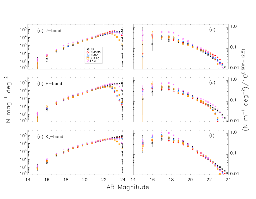
Figure 1.— (a-c) Raw galaxy counts in each of our five fields. $J-$band counts are shown in (a), $H-$band in (b) and $K_{s}-$band in (c). Error bars represent 1 $\sigma$ Poisson fluctuations. (d-f) The same data as in (a-c) divided through by an arbitrary normalized Euclidean model to expand the ordinate.

Our survey covers $\sim 3$ deg² in $J$ and $H$ and nearly $4$ deg² in $K_{s}$. However, only 1.8 deg² is covered simultaneously in all 3 bands. As shown in Section 5.1, we reliably separate stars from galaxies at $JHK_{s}<17.5$ by morphology alone. As such, for $JHK_{s}<17.5$ we count galaxies over the entire extent of our survey to achieve the best counting statistics possible. For $JHK_{s}>17.5$ we switch to counting galaxies over only the 1.8 deg² of overlap in all three bands in order to also employ color-selection techniques in separating stars from galaxies.

We constructed the galaxy counts by first making several cuts to the output catalog of SExtractor. We excluded objects in masked areas as described in Section 4. We identified stars by the methods described in Section 5.1. The raw counts for $JHK_{s}<24$ are shown in Figure 1, and the raw counts for $JHK_{s}<22$, where all fields are highly complete, are given in tabular form in Tables 4-6.

We binned identified galaxies in variable sized bins using large (1 magnitude) bins at bright magnitudes and decreasing to small (0.25 magnitude) bins at faint magnitudes. This scheme of decreasing the bin size toward fainter magnitudes allowed us to provide better statistics on the bright end of the galaxy counts curve and better resolution on the faint end. We divided the bin totals by the unmasked area of the image. We determined Poissonian galaxy count errors (1 $\sigma$) using the counting confidence limits of Gehrels (1986).

Table 4$J-$band Raw Galaxy Counts

Mag(AB)	log$(N)~{}mag^{-1}\rm{deg}^{-2}\pm 1\sigma$
	CDF-N	CLANS	CLASXS	SSA13	A370
15.000	1.134$\pm$ 0.361	0.105$\pm$ 0.518	0.236$\pm$ 0.518	0$\pm$ 0.265	1.133$\pm$ 0.225
16.000	1.310$\pm$ 0.293	1.717$\pm$ 0.063	1.651$\pm$ 0.077	1.751$\pm$ 0.163	1.756$\pm$ 0.085
17.000	2.230$\pm$ 0.079	2.303$\pm$ 0.033	2.241$\pm$ 0.041	2.260$\pm$ 0.073	2.483$\pm$ 0.039
17.750	2.564$\pm$ 0.067	2.744$\pm$ 0.035	2.716$\pm$ 0.035	2.698$\pm$ 0.060	2.954$\pm$ 0.031
18.250	2.907$\pm$ 0.046	2.939$\pm$ 0.028	2.862$\pm$ 0.030	2.974$\pm$ 0.045	3.203$\pm$ 0.023
18.750	3.054$\pm$ 0.039	3.178$\pm$ 0.022	3.092$\pm$ 0.023	3.119$\pm$ 0.038	3.371$\pm$ 0.019
19.250	3.321$\pm$ 0.029	3.391$\pm$ 0.017	3.339$\pm$ 0.017	3.270$\pm$ 0.032	3.506$\pm$ 0.016
19.750	3.593$\pm$ 0.021	3.568$\pm$ 0.014	3.550$\pm$ 0.014	3.522$\pm$ 0.024	3.701$\pm$ 0.013
20.250	3.763$\pm$ 0.018	3.800$\pm$ 0.010	3.750$\pm$ 0.011	3.708$\pm$ 0.020	3.851$\pm$ 0.011
20.750	3.962$\pm$ 0.014	3.962$\pm$ 0.009	3.971$\pm$ 0.008	3.925$\pm$ 0.015	4.033$\pm$ 0.009
21.125	4.060$\pm$ 0.018	4.109$\pm$ 0.010	4.115$\pm$ 0.010	4.077$\pm$ 0.018	4.183$\pm$ 0.010
21.375	4.159$\pm$ 0.016	4.200$\pm$ 0.009	4.218$\pm$ 0.009	4.208$\pm$ 0.015	4.273$\pm$ 0.009
21.625	4.228$\pm$ 0.015	4.277$\pm$ 0.008	4.344$\pm$ 0.008	4.374$\pm$ 0.013	4.363$\pm$ 0.008
21.875	4.311$\pm$ 0.013	4.379$\pm$ 0.007	4.448$\pm$ 0.007	4.436$\pm$ 0.012	4.444$\pm$ 0.008

Table 5$H-$band Raw Galaxy Counts

Mag(AB)	log$(N)~{}mag^{-1}\rm{deg}^{-2}\pm 1\sigma$
	CDF-N	CLANS	CLASXS	SSA13	A370
15.000	0.609$\pm$ 0.518	0.983$\pm$ 0.163	1.071$\pm$ 0.163	0$\pm$ 0.265	1.038$\pm$ 0.255
16.000	1.563$\pm$ 0.163	1.792$\pm$ 0.053	1.719$\pm$ 0.063	1.948$\pm$ 0.124	1.834$\pm$ 0.079
17.000	2.281$\pm$ 0.059	2.399$\pm$ 0.027	2.290$\pm$ 0.034	2.395$\pm$ 0.062	2.566$\pm$ 0.035
17.750	2.813$\pm$ 0.051	2.818$\pm$ 0.033	2.725$\pm$ 0.035	2.868$\pm$ 0.050	3.031$\pm$ 0.028
18.250	3.034$\pm$ 0.040	3.065$\pm$ 0.025	2.925$\pm$ 0.028	3.042$\pm$ 0.041	3.261$\pm$ 0.022
18.750	3.278$\pm$ 0.031	3.262$\pm$ 0.020	3.133$\pm$ 0.022	3.169$\pm$ 0.036	3.380$\pm$ 0.019
19.250	3.520$\pm$ 0.023	3.458$\pm$ 0.016	3.375$\pm$ 0.017	3.419$\pm$ 0.027	3.555$\pm$ 0.015
19.750	3.696$\pm$ 0.019	3.665$\pm$ 0.012	3.576$\pm$ 0.013	3.613$\pm$ 0.022	3.750$\pm$ 0.012
20.250	3.917$\pm$ 0.015	3.882$\pm$ 0.009	3.797$\pm$ 0.010	3.835$\pm$ 0.017	3.907$\pm$ 0.010
20.750	4.080$\pm$ 0.012	4.051$\pm$ 0.008	3.986$\pm$ 0.008	4.011$\pm$ 0.014	4.138$\pm$ 0.008
21.125	4.193$\pm$ 0.015	4.187$\pm$ 0.009	4.131$\pm$ 0.010	4.191$\pm$ 0.016	4.300$\pm$ 0.009
21.375	4.289$\pm$ 0.014	4.281$\pm$ 0.008	4.224$\pm$ 0.009	4.298$\pm$ 0.014	4.397$\pm$ 0.008
21.625	4.375$\pm$ 0.012	4.366$\pm$ 0.008	4.312$\pm$ 0.008	4.365$\pm$ 0.013	4.492$\pm$ 0.007
21.875	4.444$\pm$ 0.011	4.443$\pm$ 0.007	4.394$\pm$ 0.007	4.419$\pm$ 0.012	4.585$\pm$ 0.006

Table 6$K-$band Raw Galaxy Counts

Mag(AB)	log$(N)~{}mag^{-1}\rm{deg}^{-2}\pm 1\sigma$
	CDF-N	CLANS	CLASXS	SSA13	A370
15.000	1.047$\pm$ 0.361	1.028$\pm$ 0.176	0.976$\pm$ 0.176	0.900$\pm$ 0.204	1.139$\pm$ 0.155
16.000	1.649$\pm$ 0.176	1.951$\pm$ 0.050	1.763$\pm$ 0.057	1.794$\pm$ 0.059	2.003$\pm$ 0.048
17.000	2.444$\pm$ 0.057	2.634$\pm$ 0.023	2.585$\pm$ 0.023	2.575$\pm$ 0.025	2.752$\pm$ 0.020
17.750	2.934$\pm$ 0.045	2.914$\pm$ 0.029	2.818$\pm$ 0.032	2.955$\pm$ 0.046	3.182$\pm$ 0.024
18.250	3.188$\pm$ 0.034	3.152$\pm$ 0.022	3.038$\pm$ 0.025	3.107$\pm$ 0.039	3.375$\pm$ 0.019
18.750	3.425$\pm$ 0.026	3.418$\pm$ 0.016	3.317$\pm$ 0.018	3.396$\pm$ 0.028	3.502$\pm$ 0.016
19.250	3.683$\pm$ 0.019	3.609$\pm$ 0.013	3.507$\pm$ 0.014	3.602$\pm$ 0.022	3.698$\pm$ 0.013
19.750	3.864$\pm$ 0.016	3.821$\pm$ 0.010	3.722$\pm$ 0.011	3.736$\pm$ 0.019	3.846$\pm$ 0.011
20.250	4.018$\pm$ 0.013	3.978$\pm$ 0.008	3.890$\pm$ 0.009	3.932$\pm$ 0.015	3.995$\pm$ 0.009
20.750	4.110$\pm$ 0.012	4.108$\pm$ 0.007	4.021$\pm$ 0.008	4.087$\pm$ 0.013	4.147$\pm$ 0.008
21.125	4.252$\pm$ 0.014	4.219$\pm$ 0.009	4.130$\pm$ 0.010	4.239$\pm$ 0.015	4.243$\pm$ 0.010
21.375	4.271$\pm$ 0.014	4.288$\pm$ 0.008	4.222$\pm$ 0.009	4.276$\pm$ 0.014	4.329$\pm$ 0.009
21.625	4.370$\pm$ 0.012	4.344$\pm$ 0.008	4.298$\pm$ 0.008	4.385$\pm$ 0.013	4.372$\pm$ 0.008
21.875	4.423$\pm$ 0.012	4.412$\pm$ 0.007	4.378$\pm$ 0.007	4.420$\pm$ 0.012	4.449$\pm$ 0.008

We then performed a weighted average of galaxy counts over all fields. We created the weighted average by taking into account Poisson errors (weight $=1/\sigma^{2}$). This ensures that results from the widest fields in our survey carry more weight on the bright end.

5.1. Star-Galaxy Separation

We used a combination of morphology and color to separate stars from galaxies for our galaxy counts. Our methods include use of the SExtractor “CLASS_STAR” parameter, the ratio of semimajor to semiminor axes of objects, and $J-K_{s}$ color to separate stars from galaxies. We honed our methods on a group of spectroscopically identified stars and galaxies in the GOODS-N (a subfield of the CDF-N). This involved the use of $J$ and $K_{s}-$band catalogs from this study and the GOODS-N redshift catalog from Barger et al. (2008). Finally, as an independent test of our methods, in the four of our five fields (all but A370) where we overlap with the SDSS, we compared our classified stars having $JHK_{s}<19$ with the morphological classifications for these objects in the SDSS catalogs. The results of these methods are discussed below. Our final star counts generated using these methods are shown in Figure 2

The CLASS_STAR parameter is an output of SExtractor to describe whether a given object looks like a point source or an extended source. The CLASS_STAR output contains a value between 0 (extended object) and 1 (point source) and is assigned by SExtractor to each object detected in the image. CLASS_STAR can be used to separate stars from galaxies at bright magnitudes, but the accuracy of this parameter breaks down at fainter magnitudes. Where that breakdown occurs depends on the depth of the field and the SEEING_FWHM input parameter (see Table 2).

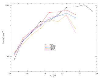
Figure 2.— Star counts for each of our fields using the combination of morphology and color criteria described in Section 5.1

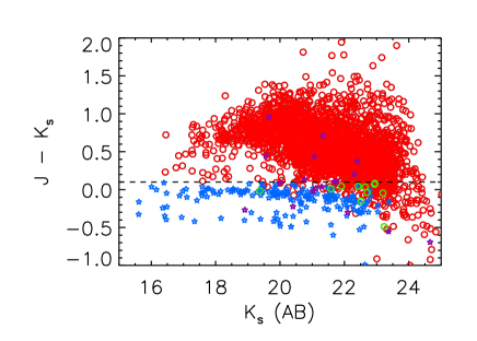
Figure 3.— $J-K_{s}$ color-magnitude plot for spectroscopically identified stars and galaxies in the GOODS-N region (a subfield of the CDF-N) from the catalog of Barger et al. (2008). Accurately identified stars are shown in blue. Stars we fail to identify are shown in purple. Accurately identified galaxies are shown in red circles and galaxies misidentified as stars are in green circles. The vast majority of stars are found below the line $J-K_{s}=0.1$.

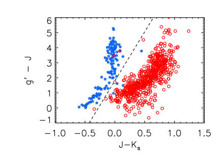
Figure 4.— A color-color plot demonstrating the utility of a combination of the SDSS $g^{\prime}$ filter with the $J$ and $K_{s}$ filters in the NIR for star-galaxy separation. Stars are shown as blue stars and galaxies as red circles from the spectroscopic catalog of Barger et al. (2008). We use the $g^{\prime}$$JK_{s}$ color-color data from our fields that overlap with the SDSS to investigate discrepancies between our star-galaxy separation and that of the SDSS, as described in Section 5.1

The SEEING_FWHM input parameter is provided to SExtractor by the user to describe the average point source Full-Width-Half-Maximum (FWHM) in the image. This parameter is critical for SExtractor to accurately identify stars with its output parameter CLASS_STAR.

We determined the optimal value for the SEEING_FWHM input parameter by first running SExtractor on an image to determine the FWHM of point sources in the image (using an initial guess at the image seeing for the input SEEING_FWHM). We then took the median FWHM for selected point sources (CLASS_STAR $>0.95$) as the final input value for the SEEING_FWHM parameter. Values calculated in this way for the SEEING_FWHM parameter in each field are listed in Table 3.

We found that on occasion for bright galaxies the CLASS_STAR parameter misidentified galaxies as stars that were clearly galaxies by eye (2 out of 125 galaxies at $K_{s}<19$ in the GOODS-N catalog). We resolved this issue by constraining the ratio of semimajor to semiminor axis for stars ($a/b\leq 1.3$).

Using the star identification criteria of CLASS_STAR $>0.7$ for $JK_{s}<17.5$ and CLASS_STAR $>0.9$ and $a/b\leq 1.3$ for $17.5<JK_{s}<19$, we correctly identified $100\%$ of stars for $JK_{s}<19$ from the spectroscopic sample of Barger et al. (2008).

To extend our star-galaxy separation to fainter magnitudes, we used a combination of the SExtractor CLASS_STAR parameter and the $J-K_{s}$ color of objects. We determined that a color cut of $J-K_{s}<0.1$ and CLASS_STAR $>0.95$ for $19<JK_{s}<24$ accurately identified $>90$% of stars while only misclassifying $<1$% of galaxies as stars. Because galaxies dominate the counts at these faint magnitudes, the combination of these effects introduces less than 1% error in the counts in the range $19<JK_{s}<24$. These results are displayed in Figure 3 where $K_{s}-$band magnitude is plotted against $J-K_{s}$ color for the Barger et al. (2008) sample. Blue stars show correctly identified stars, red circles show correctly identified galaxies, and purple stars and green circles show misclassified stars and galaxies, respectively.

In our fields that overlap with SDSS (all but A370), we were able to perform a check on our bright $(JHK_{s}<19)$ star selection by cross-correlating with objects classified morphologically as point sources in SDSS. We looked at two things in this analysis. First, we searched for objects that we identifed as stars which were classified as extended objects in SDSS. Second, we searched for objects that we found to be galaxies that were classified as point sources in SDSS.

For $JHK_{s}<17.5$, we found that none of our galaxies were listed as point sources in SDSS. However, a handful (5-15) of our stars in each field were listed as extended sources in SDSS. We first investigated this discrepancy by eye and found that many of these objects were clearly point sources in our images identifiable by their diffraction spikes. This is perhaps due to the fact that our images are much deeper than SDSS, or these are late-type stars that are brighter in the NIR than in the optical. Other sources appeared to be close binary point sources in our images, perhaps unresolved by the SDSS. Given that the majority of discrepant point sources appear to be misclassifications in the SDSS, we conclude that we have done a robust job of star-galaxy separation for $JHK_{s}<17.5$.

In the range $17.5<JHK_{s}<19$, we found $>90$% agreement between objects we classfied as stars and point sources identified by SDSS, as well as for objects we classified as galaxies and their SDSS counterparts. To investigate discrepant sources, we employed $g^{\prime}$(sdss) $-J$ versus $J-K_{s}$ color-color diagrams. The utility of such diagrams for separating stars and galaxies is shown in Figure 4 using the Barger et al. (2008) sample as an example, where SDSS counterparts are found for 131 stars and 647 galaxies. Using this sample, we determined that a color cut of $g^{\prime}-J>6.5\times(J-K_{s})+1.8$ was appropriate for selecting the vast majority of stars.

We plotted objects we identified as stars, but whose SDSS counterparts were classified as extended on the $g^{\prime}JK_{s}$ plane and found that the majority matched the color criterion for stars defined above. Those that did not meet the criterion typically had very high SExtractor CLASS_STAR parameters in our catalogs and, as such, are likely candidates to be late-type M and L dwarf stars.

Finally, we plotted objects that we identified as galaxies but whose SDSS counterparts were classified as point sources on the $g^{\prime}JK_{s}$ plane. We found a minority of these objects did, in fact, meet the $g^{\prime}JK_{s}$ color criterion for stars. In this case, we flagged these objects as stars in our catalogs. Stars identified in this way through comparison with the SDSS were very few in number and only affect the galaxy counts in the $17.5<JHK_{s}<19$ range on the $\sim 0-3$% level.

The SDSS does not cover our A370 field, so we do not have the opportunity to compare our star-galaxy separation with an independent optical morphology classification like we have done for the other fields. Based on our comparison with the SDSS in other fields, we expect that stars we may have missed in the A370 field could contribute to an excess on the few percent level to counts in the $17.5<JHK_{s}<19.$ range.

As seen in Figure 3, there are stars that will be missed by our color cut in $J-K_{s}$. These will tend to be M and L dwarf stars because they are redder than the rest of the main sequence population (T dwarfs, in fact, have $J-K_{s}<0$ like typical main sequence stars). However, we would expect to identify the majority of M and L dwarfs as stars based on morphology alone for $K_{s}<19$ (as demonstrated above), corresponding to distances of out to $\sim 100$ parsecs. Beyond this we would miss these faint dwarf stars in our star removal.

The space density of M and L dwarfs is poorly constrained at large heliocentric distances, but Stanway et al. (2008) and Pirzkal et al. (2009) have shown that M and L dwarfs may exist in large numbers out to several kpc into the Galactic halo. The star counts for M dwarfs from these two groups roughly agree and appear flat out to very faint magnitudes at levels of $\sim 100-200$ mag^-1 deg².

In our galaxy counts, assuming the worst case scenario, this could represent a 15% systematic error in the brightest bin ($K_{s}=19-20$), for which we require $J-K_{s}<0.1$. Assuming flat star counts for these late-type dwarf stars, this error would drop to $<10$% at $K_{s}=20.5$ and $<5$% at $K_{s}=21.5$. The focus of this paper is the bright galaxy counts for which we believe our star-galaxy separation is robust, but we alert the reader that the counts remain uncorrected for late-type dwarf stars fainter than $JHK_{s}=19$.

6. Bright Galaxy Counts and Local Large Scale Structure

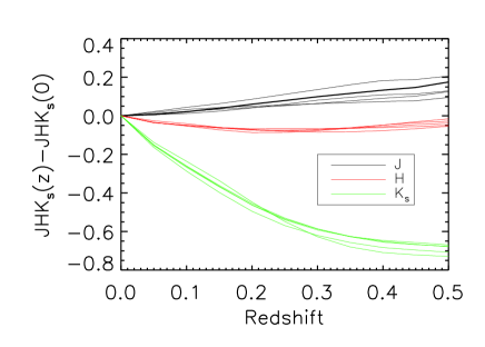
Figure 5.— NIR $K-$corrections are shown as a function of redshift in $J$ (black), $H$ (red), and $K_{s}$ (green), from Mannucci et al. (2001). Five galaxy types (E, S0, Sa, Sb, Sc) are shown (though not identified individually) to demonstrate the similarity in each NIR bandpass of the $K-$correction for different galaxy types. Because of this similarity the uncertainty in type mixture in our galaxy counts only leads to uncertainties of $<0.005$ in the determination of the expected Euclidean slope.

Figure 6.— The distance of galaxies at a given $K_{s}-$band magnitude (the distributions are very similar in $H$ and $J-$band) assuming homogeneity and a non-evolving NIR luminosity function. This distance distribution was calculated using the NIR luminosity functions of Jones et al. (2006) and the $K-$corrections of Mannucci et al. (2001). The plotted points show the peak of the distance distribution ($M^{*}$) in a given magnitude bin, and the error bars show one standard deviation above and below the peak in each bin.

In the past two decades, numerous NIR galaxy counts studies have been published. Typically new data are overplotted with a selection of previous works to demonstrate how the various studies agree or disagree in a given bandpass. At bright magnitudes, factors of two or more discrepancy between any two studies are not uncommon in these comparisons. A lack of knowledge about the proper normalization of the galaxy counts curve makes it difficult to determine when such differences are actually due to variations in large scale structure and not other effects, such as differences or inconsistencies in photometry.

The slope of the bright galaxy counts curve, on the other hand, is a measure of local large scale structure that is independent of the normalization. In a static, homogeneous, Euclidean universe, galaxy counts would follow the curve $N=A\times 10^{\alpha m},$ where $A$ is a normalization constant, $\alpha=0.6$, and $m$ is apparent magnitude. A slope of $\alpha=0.6$ is also expected for the bright end of the galaxy counts curve in an expanding, homogeneous universe where $K-$corrections are small and nearly independent of galaxy type and where cosmological effects on the luminosity distance are small.

Barro et al. (2009) show that for galaxy counts derived from Schechter (1976) luminosity functions, the bright counts slope is expected to follow the Euclidean prediction and be dominated by $M\leq M^{*}$ galaxies until a transition to lower slope is induced by the knee in the luminosity function around $JHK_{s}\sim 17.5$.

The bright counts slope is then modified by the $K-$corrections in a given bandpass, which act effectively as a changing $M^{*}$. Optical $K-$corrections are large and galaxy type dependent, and thus considerations of large scale structure based on the slope of optical galaxy counts are plagued with uncertainties about the exact mix of galaxy types in the counts. NIR $K-$corrections are smaller than in the optical and nearly type independent. Figure 5 shows the low-redshift $K-$corrections from Mannucci et al. (2001) ($J$ in black, $H$ in red, and $K_{s}$ in green). These are shown for five galaxy types (E, S0, Sa, Sb, Sc), demonstrating the near type independence of the NIR $K-$corrections.

It is straightforward to determine the effect of the $K-$corrections of Mannucci et al. (2001) on the theoretical slope of the galaxy counts curve in a homogeneous distribution of galaxies in the nearby expanding universe ($z<0.1$, $cz=H_{0}D$). Assuming $H_{0}=70~{}\rm{km}~{}\rm{s}^{-1}~{}\rm{Mpc}^{-1}$ and an equal mix of all five galaxy types shown in Figure 5, the slope for the $J-$band should be $\alpha\sim 0.57$, for the $H-$band $\alpha\sim 0.58$, and for the $K_{s}-$band, $\alpha\sim 0.61$. Because of the similarity of the $K-$corrections across galaxy types the uncertainty introduced by the lack of knowledge of the exact type mixture in the calculation of the expected slope is less than $\pm 0.005$. This result is also independent of the shape of the galaxy luminosity function if one assumes no galaxy evolution at $z<0.1$. In Figure 6 we show the distribution in distance of galaxies for a range of $K_{s}-$band magnitudes.

In what follows, we consider departures of $\sim 0.01-0.1$ from the Euclidean prediction . If we ignore evolution and treat the slope as a direct measure of local large scale structure, these departures can be thought of as changes in the space density of galaxies as one moves further out into the local universe. For example, a difference of $0.01$ from the Euclidean predication measured over an interval of three magnitudes would roughly imply a galaxy space density change of $\sim 7$% over the range of distances sampled at those magnitudes. As shown in Figure 6, the range of distances sampled in any given magnitude bin increases toward fainter magnitude, adding uncertainty to the physical significance of a change in slope, but if the luminosity function is truly a constant over the range measured, then the slope is a measure of the space density of galaxies over that range.

Maddox et al. (1990) found a steeper than Euclidean slope in $B-$band counts over the 4300 deg² of the Automated Plate Measuring (APM) galaxy survey and suggested rapid galaxy evolution at low redshifts as an explanation. Koo & Kron (1992) point out that dramatic collective evolution near the present epoch would be unusual, and they instead attribute the steep slope of the APM survey counts to some combination of model uncertainties and normal evolution. Shanks (1990) point out that the steep galaxy counts slope could be due to clustering if we are located inside a large ($\sim 150h^{-1}$ Mpc) region of $\sim 50$% underdensity. However, as mentioned above, optical $K-$corretions are highly type dependent, so a measurement of the slope in the NIR is required for a more reliable test of local large scale structure.

Huang et al. (1997) found a steeper than Euclidean slope ($\alpha=0.69$) in $K_{s}-$band counts over a collection of fields totalling $\sim 10$ deg², but they point out that the amount of evolution needed to account for the effect, particularly in the NIR at low redshifts, seems unlikely. The alternative to rapid evolution cited by Huang et al. (1997), is a $\sim 50$% local underdensity of galaxies stretching 300$h^{-1}$ Mpc in extent. They point out that this would mean local measurements of the cosmological mass density, $\Omega_{0}$, would be low by the same factor and that local measurements of $H_{0}$ could be high by as much as 33%. Evidence for such a “local void” using 2MASS, the Two-degree Field Galaxy Redshift Survey (2dFGRS), and other data, along with galaxy counts models, has been presented in Busswell et al. (2004) and Frith et al. (2003, 2005). In what follows, we look at the bright galaxy counts slope of our data in combination with 2MASS, the variability in the slope as a function of position on the sky, and possible implications for local large scale structure.

6.1. Galaxy Counts in the 2MASS XSC

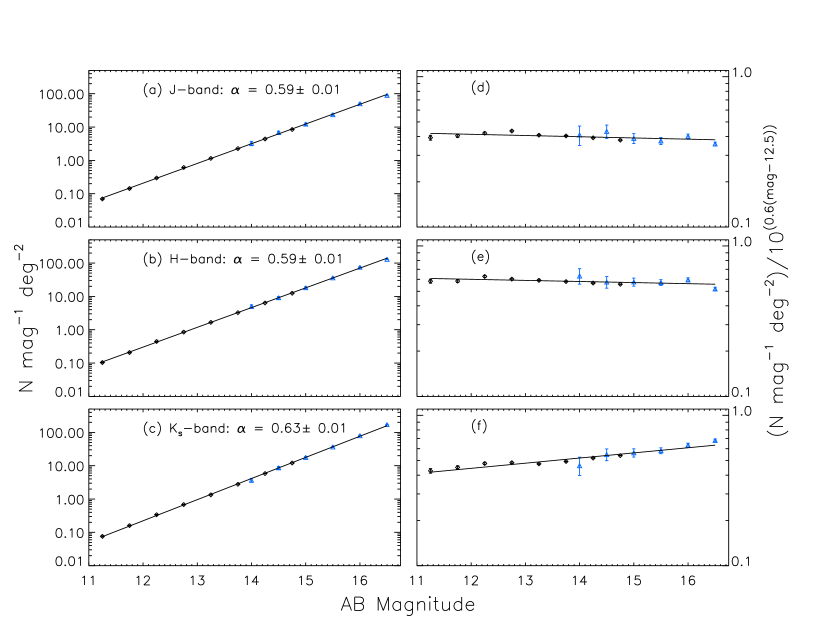
Figure 7.— (a-c) Average counts for 2MASS $|\rm{b}|>30$ (black diamonds) and for 2MASS-6x Lockman Hole (blue triangles). Error bars show 1 $\sigma$ Poisson fluctuations (smaller than plot symbols in a-c). (d-f) are the same data as (a-c) after having been divided through by a normalized Euclidean model (i.e., $[N~{}mag^{-1}\rm{deg}^{-2}]/10^{0.6(\rm{m}-12.5)}$). Solid lines show an error-weighted least-squares fit to the counts. The calculated slopes are listed in the plots.

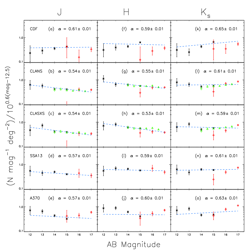
Figure 8.— (a-e) $J-$band counts for 2MASS (black asterisks) vs. counts from this study in each field (red diamonds). Green triangles represent the counts from the 2MASS-6x survey, which overlaps with the CLANS and CLASXS fields. (f-j) $H-$band counts in the same format. (k-o) $K_{s}-$band counts in the same format. The blue dashed lines represent an error-weighted least squares fit to the data, and the calculated slope is listed in each plot. The counts have been divided through by a normalized Euclidean model to expand the ordinate.

We downloaded the entire 2MASS extended source catalog (XSC) and 2MASS-6x XSC from the NASA/IPAC Infrared Science Archive. We constructed 2MASS galaxy counts from the catalog over an area of $\sim 20,000$ deg² representing the entire 2MASS XSC for Galactic latitude $|b|>$ 30 (2$\pi$ Steradians). We limited this 2MASS sample to $JHK_{s}<15.5$ to stay within the all sky catalog’s completeness limits. We excluded known 2MASS Galactic extended sources from the counts using the Galactic extended source catalog available at NASA/IPAC website. As shown in Figure 6, galaxy counts from 2MASS from 11-15^th magnitude are sampling $M^{*}$ galaxies in the local universe at distances of $\sim 50-350$ Mpc.

We also constructed galaxy counts from the 2MASS-6x (Beichman et al. 2003) catalog of extended sources in the $\sim 25$ deg² centered on the Lockman Hole area of low galactic HI column density (Lockman et al. 1986). These data represent 25 deg² where 2MASS observed six times as long as the all sky catalog exposure times, thus making the 2MASS-6x catalog roughly one magnitude deeper in $J,H$ and $K_{s}$. We were able to further “deepen” the 2MASS-6x Lockman Hole catalog because our deep data in the CLANS and CLASXS fields overlaps 100% with the 2MASS-6x Lockman Hole. As such, we were able to measure completeness in the 2MASS-6x catalog, and correct the counts to $JHK_{s}=16.75$. Thus, we use the 2MASS and 2MASS-6x catalogs to firmly establish average galaxy counts on the bright end. The average 2MASS galaxy counts for $|b|>30$ deg are shown in Figure 7.

The solid lines in Figure 7 show an error-weighted least squares fit to the data. In the left panels the counts are shown in the standard $N$ vs. magnitude form, and in the right panels the counts are shown divided through by a normalized Euclidean model. For this global average of galaxy counts in $J$, $H$, and $K_{s}$ we find $\alpha=0.59,0.59$, and $0.63~{}(\sim\pm 0.01$ in all three bands), respectively. These values are all 0.01-0.02 above the Euclidean prediction, representing a possible galaxy space density increase toward fainter magnitudes of 7-15% over the magnitude range sampled.

Next, we extracted 2MASS counts for areas of $\sim 25$ deg² centered on each of our fields. In Figure 8 we show our raw counts (red diamonds) for $JHK_{s}<17.5$ plotted with 2MASS counts (black asterisks) from each of these 25 deg² subfields. The dashed lines show an error-weighted least-squares fit to the data. In the CLANS and CLASXS fields we include our counts extracted from the 2MASS-6x survey (green triangles), because these two fields lie within the 2MASS-6x Lockman Hole. The counts have been divided through by a normalized Euclidean model ($\alpha=0.6$). The calculated slopes are tabulated in the plots. We note that in many cases fitting to only the data points from this study would yield a much steeper slope than that obtained with the inclusion of 2MASS. In this measurement of the local slope at our field positions, we find a mix of values ranging from sub-Euclidean to super-Euclidean. We note that the most sub-Euclidean slopes are found in our fields near the supergalactic equator (CLANS and CLASXS). We return to this point in Section 6.2.

In Figure 9, we show the error-weighted average of our counts (red squares) alongside the error-weighted average of the 2MASS counts (black diamonds) extracted from the 25 deg² subfields centered on our fields (for a total of 125 deg²), as well as the counts from the 2MASS-6x Lockman Hole (green triangles). Again, we fit the slope with an error-weighted least-squares method and the slopes are listed in the plots. We find that, on average, when combined with 2MASS, our counts yield a Euclidean slope within our error bars of $\pm 0.01$. We note that taken on their own, our counts in both the $H$ and $K_{s}-$bands would appear super-Euclidean. This is likely due simply to a lack of bright objects in the fields ($HK_{s}\sim 15$), leading to large random errors in the brightest bin.

6.2. Galaxy Counts and the Supergalactic Plane

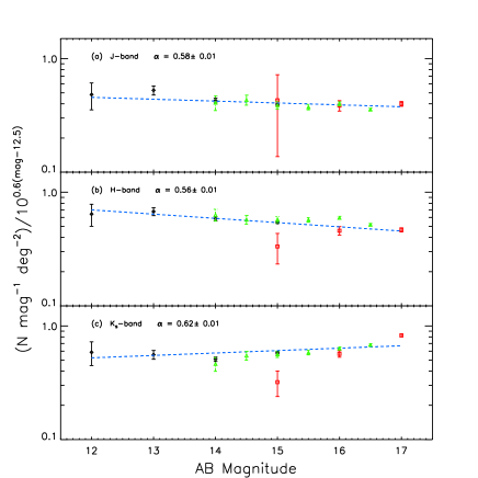
Figure 9.— Average $J$, $H$, and $K_{s}-$band counts for 2MASS subfields of 25 deg² each centered on our fields (black diamonds), 2MASS-6x Lockman Hole (green triangles), and average counts for this study (red squares). The counts have been divided through by a normalized Euclidean model to expand the ordinate.

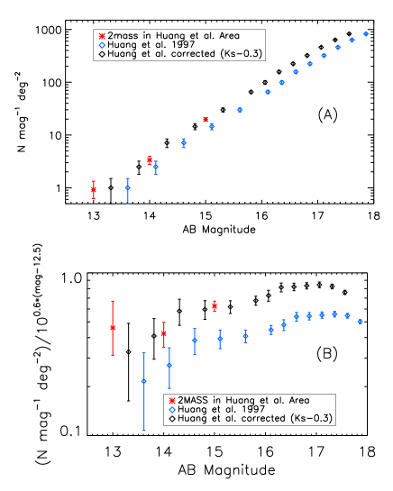
Figure 10.— (a) The Huang et al. (1997) $K_{s}$ counts are shown as blue diamonds. The 2MASS counts were constructed for the Huang et al. (1997) fields for comparison and are shown as red asterisks. After applying a zeropoint correction ($K_{s}=K_{s}-0.3$; see text) the Huang et al. counts (black diamonds) align well with the 2MASS $K_{s}$ counts from the same area. We adopt this adjustment as a correction to the Huang et al. counts, bringing them into good agreement with other studies over the same magnitude range. Error bars show 1 $\sigma$ Poisson fluctuations. (b) The same data as in (a) but divided through by a normalized Euclidean model (i.e. $[\rm{N}mag^{-1}deg^{-2}]/10^{0.6(K_{s}-12.5)}$).

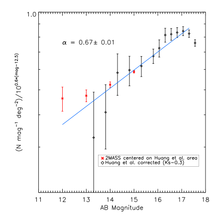
Figure 11.— (a) The Huang et al. (1997) $K_{s}$ counts are shown as black diamonds after a zeropoint correction ($K_{s}-0.3$; see text). The 2MASS counts were constructed from 25 deg² subfields (375 deg² total) centered on the Huang et al. (1997) fields for comparison and are shown as red asterisks. The line shows an error-weighted least-squares fit to the data. We find $\alpha=0.67$ in this fit, a slightly lower number than was found for the Huang et al. (1997) data alone ($\alpha=0.69$), but still distinctly super-Euclidean.

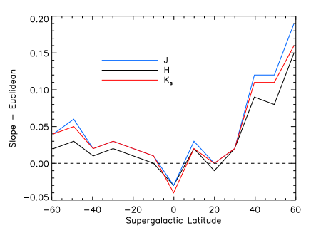
Figure 12.— Average slope as a function of supergalactic latitude (SGB) for the 2MASS counts ($|\rm{b}|>30;10.5<JHK_{s}<15.5$). The expected Euclidean slope has been subtracted from the measured values such that the dashed horizontal line at 0 represents the Euclidean expectation in all bands. $J-$band appears in blue, $H$ in black, and $K_{s}$ in red. Northern SGB slopes show a strong trend toward super-Euclidean, generally consistent with results from Huang et al. (1997) and Gardner et al. (1993). The only distinctly sub-Euclidean slopes appear at SGB $\sim 0$, consistent with our findings in the CLANS and CLASXS fields which lie near the supergalactic equator.

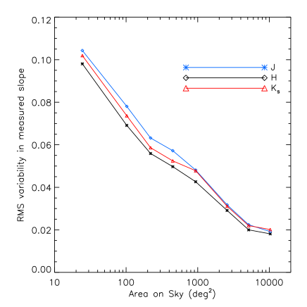
Figure 13.— The 2MASS $|\rm{b}|>30$ sky was divided up into increasingly larger patches of area on the sky ranging from $\sim 25-10000~{}\rm{deg}^{2}$ to test for when the rms variability in slope between sub-areas was reduced to the order of the variability induced by the supergalactic plane alone. The rms variability in measured slope is shown as a function of the area of the patches of sky. The result is that for patches of sky greater than $\sim 1000$ deg², the variability in the slope can be accounted for by the supergalactic plane alone, such that other local large scale structure has been sufficiently averaged out.

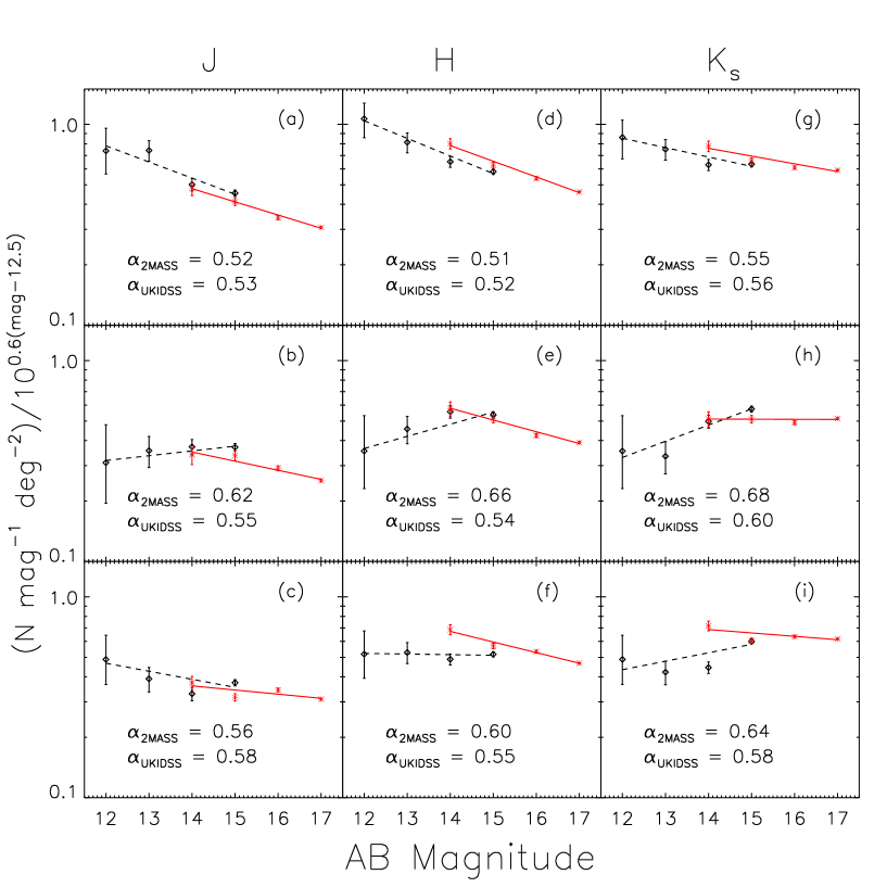
Figure 14.— The slope of the 2MASS counts (black diamonds) in the range $11.5<JHK_{s}<15.5$ compared with the slope of the UKIDSS counts (red asterisks) in the range $13.5<JHK_{s}<17.5$. (a-c) show $J-$band counts, (d-f) show $H-$band counts, and (g-i) show $K_{s}-$band. The top row of plots is for subfield 1, the middle for subfield 2, and the bottom for subfield 3 (see Table 8 for subfield details). The dashed and solid lines show an error-weighted least-squares fit to the 2MASS and UKIDSS counts, respectively. The slopes for each are given on the plots and fitted errors on the slopes are $\sim 0.01$ in all cases. The result is that for three large fields totalling $\sim 135$ deg² at high supergalactic latitude, no abrupt steepening of the counts slope is seen.

We now consider the implications of our bright galaxy counts in terms of local large scale structure. The most striking feature in the local large scale structure is the supergalactic Plane discovered by de Vaucouleurs 1953. The plane is roughly perpendicular to our Galactic plane. In Figure 8, we find that in the CLANS and CLASXS fields, the slope appears distinctly sub-Euclidean, whereas in the other three fields the slopes are closer to the Euclidean prediction. This is interesting because the CLANS and CLASXS fields are of nearly equatorial supergalactic latitude ($-1.8$ and $-3.9$ deg, respectively; see Table 1). In fact, all of our fields are at relatively low absolute supergalactic latitude (average $|\rm{SGB}|\sim 10$ deg), with A370 being the furthest off the plane at $-25.7$ deg.

The fields of Huang et al. (1997), where a strong super-Euclidean slope was found in the $K_{s}-$band, span absolute supergalactic latitudes from $10<\rm{SGB}<54$ with an average of $\rm{SGB}\sim 30$ deg. As a verification of the Huang et al. (1997) result, we did another comparison in which we extracted 2MASS galaxies from patches of 25 deg² centered on the Huang et al. (1997) fields. First, however, we extracted 2MASS counts from the actual areas of the Huang et al. (1997) fields and found a zeropoint offset of $-0.3$ to their counts. We show this in Figure 10. We applied this offset to their counts before proceeding with the comparison to the larger (25 deg²) fields.

We plot the zeropoint-adjusted counts from Huang et al. (1997) with the average of 2MASS counts over the larger surrounding areas in Figure 11. We calculate a slope of $\alpha=0.67$ for the combined dataset. This value is slightly smaller than that found using just the Huang et al. (1997) datapoints ($\alpha=0.69$), but still distinctly super-Euclidean. Over the magnitude range sampled, this would still represent roughly a factor of two increase in the space density of galaxies as found by Huang et al. (1997).

Gardner et al. (1993) found a super-Euclidean bright counts slope of $\alpha=0.67$ in their survey of a collection of fields totalling $\sim 10$ deg² at an average absolute SGB of $\sim 25$. Väisänen et al. (2000) found a sub-Euclidean slope at bright magnitudes in the $K_{s}-$band at high supergalactic latitude ($\rm{SGB}=40$), but this can likely be explained by the fact that they had three Abell clusters in their fields (A2168 at $z=0.06$; A2211 at $z=0.15$; and A2213 at $z=0.15$), which likely dominate their galaxy counts at bright magnitudes. The effect of just one galaxy cluster in a similar sized field can be observed in our data in Figure 1, where the A370 ($z=0.37$) counts show a large excess in the range $17<JHK_{s}<19$. The three lower redshift clusters in the Väisänen et al. (2000) fields would produce large excesses at brighter magnitudes, and indeed they find their counts to be in excess over all other published studies at bright magnitudes.

Thus, from the evidence above, it seems that a large fraction of the variability in the slope and absolute numbers between different bright counts studies can be attributed to nearby large scale structure, be it individual galaxy clusters or local superstructure. When individual nearby galaxy clusters are avoided, there appears to be evidence for the slope of bright galaxy counts to be related to supergalactic latitude.

To investigate this further, we calculated the bright counts slope in 2MASS as a function of position on the sky by dividing the $|\rm{b}|>30$ catalog into slices in supergalactic latitude ranging in area from $\sim 500-2500$ deg² each. As a result, we obtained slope measurements in $J$, $H$, and $K_{s}$ for $-60<\rm{SGB}<60$. We plot the average 2MASS slope as a function of SGB in Figure 12. In this figure the Euclidean slope prediction has been subtracted from the measured values such that the dashed horizontal line represents the expectation for a Euclidean slope in all three bands. $J$-band is represented in blue, $H-$band in black, and $K_{s}-$band in red. The error in the slope measurements is $\sim 0.01$ in all cases. We note that the similarity in slope measurements between bands suggests that our slope determinations are robust.

In Figure 12 the only distinctly sub-Euclidean slopes are found near the supergalactic equator, consistent with results from our CLANS and CLASXS fields, with all other latitudes appearing to be super-Euclidean. At high northern supergalactic latitudes we find that slopes exceeding the Euclidean prediction by $>0.05$, such as those found by Huang et al. (1997) and Gardner et al. (1993), are typical. One interpretation of these results would be that near the supergalactic plane, the very brightest counts are populated with an excess of sources causing the slope to drop, and above the plane a relative paucity of nearby sources above the plane causing the slope to steepen. The southern supergalactic latitudes do not display the same sharp rise to super-Euclidean as in the north. The magnitude range sampled in these counts is $10.5<JHK_{s}<15.5$, which means that the brightest magnitude bin is centered on typical galaxies at a distance of $\sim 50$ Mpc. This means that toward high northern SGB, where slopes are $\sim 0.1$ above the Euclidean prediction, the space density of galaxies at a distance of $50$ Mpc could be low by roughly a factor of two compared to the space density $250-350$ Mpc distant. In the southern supergalactic cap the slopes are not as steep ($\sim 0.03$ above Euclidean), but still represent a possible underdensity of $\sim 25\%$ at $50$ Mpc relative to $250-350$ Mpc.

Next we took a broad average of 2MASS counts in and out of the supergalactic plane. In Table 7 we give the measured average slope for galaxy counts in the supergalactic plane ($|\rm{SGB}|<10$) and out of the plane. We find that on average the counts in the plane are sub-Euclidean, consistent with what we found in Figure 12. The slope out of the plane is steeper by some $\Delta\alpha\sim 0.02-0.06$ in both the northern and southern supergalactic caps, and super-Euclidean on average. Thus, the expected variability in the 2MASS bright counts slope is $\sim\pm 0.04$ due only to the very largest local structure.

We next divided the 2MASS $|\rm{b}|>30$ sky into 844 patches of $\sim 25$ deg² each. We measured the slope of the galaxy counts from $11<JHK_{s}<15$ for each and found an rms variability in the slope of $\sim 0.1$. Inside distances of $\sim 250$ Mpc, 2MASS is $1-2$ magnitudes deeper than $M^{*}$ and, as such, is measuring a fairly complete sample of the local luminosity function. This implies our 25 deg² patches are sampling structure on size scales of $\sim 20$ Mpc and find rather strong variability.

Table 7 2MASS Galaxy Counts Slope Over the Galactic Caps, the Supergalactic Equator and the Supergalactic Caps

Region	$J$ Slope	$H$ Slope	$K_{s}$ slope
Gal. $|\rm{b}|>30$ deg	0.59	0.59	0.63
$|\rm{SGB}|<10$ deg	0.55	0.57	0.59
SGB$<-10$ deg	0.60	0.59	0.63
SGB$>10$ deg	0.61	0.61	0.65
$|\rm{SGB}|>10$ deg	0.61	0.60	0.64

To test for the angular size over which all local large scale apart from the supergalactic plane could be sufficiently averaged out, we divided up the 2MASS $|\rm{b}|>30$ sky into increasingly larger subfields and measured the rms variability in the measured slope across all subfields. Figure 13 shows the result of this exercise for subfields ranging from $\sim 25-10,000$ deg². We find that when averaging over subfields larger than $\sim 1000$ deg², the rms variability between all subfields is of the same order of that induced by the supergalactic plane alone, and as such, all other local large scale structure has been sufficiently averaged out. In the 2MASS sample, this suggests that effects of local large scale structure have been sufficiently averaged out over scales of $\sim 150$ Mpc.

Based on the analysis above, we conclude that the local supergalactic plane is overdense by $10-15$% compared to regions at distances of $\sim 250-350$ Mpc, while the voids just above and below the plane are underdense by up to a factor of two relative to similarly distant regions.

Cold Dark Matter simulations such as the Millenium Run (Springel et al. 2005) predict that the largest structures in the universe should be $\leq 100$ Mpc in extent. Observed large scale structures, most notably the Sloan Great Wall (Gott et al. 2005), demonstrate the existence of structure on scales much larger than simulations predict. Consensus has not yet been reached on whether a structure like the Sloan Great Wall represents an extreme non-linearity in the matter distribution of the universe, or if inhomogeneities on several hundred Mpc scales are typical. Two recent analyses of the distribution of matter in the SDSS DR6 dataset (Sarkar et al. 2009; Kitaura et al. 2009) demonstrate the current range of interpretation of observations, in which Sarkar et al. (2009) arrive at scale of homogeneity of $70$ Mpc and Kitaura et al. (2009) claim to have discovered a new large void $150$ Mpc in diameter. Clearly the typical size of large scale structure still depends on how one interprets the data. In our analysis, we find that averaging galaxy counts over areas on the sky spanning $\sim 150$ Mpc sufficiently smooths out local structure. However, in the same data, the super-Euclidean slopes above and below the supergalactic plane suggest that the local space density of galaxies may be low by $25-100$% compared to regions a few hundred Mpc away, which would suggest that local structure exists on much larger scales than $150$ Mpc.

6.3. Comparison with the UKIDSS Large Area Survey

We employ the UKIDSS survey to investigate the possibility that the entire 2MASS volume resides in a relatively underdense region that is $\geq 250$ Mpc in radius, as suggested by Huang et al. (1997). The expectation if this were the case would be a steepening of the galaxy counts slope in the range $15<JHK_{s}<17$, as, in fact, is seen in the Huang et al. (1997) sample when compared with 2MASS.

As a test for a large void, we employ the UKIDSS (Lawrence et al. 2007) third data release (DR3; Warren et al., in preparation) Large Area Survey (LAS), which has recently become public. The DR3 LAS covers several hundred degrees of sky within the SDSS footprint to depths of $JHK_{s}\sim 19$. We selected three large subfields totalling $\sim 135$ deg² in the UKIDSS LAS. We downloaded catalogs from the WFCam Science Archive, and the range in celestial coordinates and SGB for these subfields are given in Table 8. We selected the fields to span a wide range of SGB above and below the supergalactic plane.

We cross-correlated the UKIDSS catalogs with their SDSS counterparts and removed stars from the catalogs via the SDSS classifier and $g^{\prime}$$JK$ color-color diagrams in a similar manner to what is described in Section 5.1. A comparison between the slope of the 2MASS counts and the UKIDSS counts for the three subfields is shown in Figure 14. 2MASS counts are shown in black diamonds and UKIDSS counts in red asterisks. The dashed and solid lines show error-weighted least-squares fits to the 2MASS and UKIDSS counts, respectively. The slopes for each fit are listed in the plots, and the associated errors in the fitted slopes are $\sim\pm 0.01$ in all cases.

The result is that for these three subfields, we do not observe a steepening of the slope at magnitudes beyond the 2MASS limits. In fact, in the majority of cases in Figure 14, the slope appears to be decreasing into the fainter magnitudes of the UKIDSS survey.

Table 8 Three Subfields Selected from the UKIDSS DR3 LAS

Subfield	$\Delta$RA (deg)	$\Delta$DEC (deg)	$\Delta$SGB (deg)
1	$201.5-222.1$	$9.0-11.4$	$10-30$
2	$337.5-360.0$	$-1.0-1.0$	$13-34$
3	$135.0-150.0$	$7.0-11.4$	$-(37-52)$

7. Summary

We have presented a deep, wide-field NIR survey over five widely separated fields at high galactic latitude covering a total of $\sim 3$ deg² in $J$, $H$, and $K_{s}$. The deepest parts of the survey ($\sim 0.25$ square degrees) reach 5 $\sigma$ limits $JHK_{s}>24$. As such, this is one of the deepest wide-field NIR imaging surveys to date. In this paper we focus on the bright galaxy counts slope and the implications for local large scale structure. We leave analysis of the faint galaxy counts and other applications of these data for future papers.

We measure the slope of the bright galaxy counts in our data combined with the larger 2MASS fields at our positions on the sky, and we find it consistent with the Euclidean prediction, on average, over our five fields. We note that our fields are at a low average supergalactic latitude (SGB $\sim 10$) and our fields near the supergalactic equator show a sub-Euclidean slope. In the 2MASS $|\rm{b}|>30$ sky, we find the slope of the counts to be sub-Euclidean near the supergalactic equator and super-Euclidean at all other SGB. This is consistent both with our measured slope near the supergalactic equator and with other studies that have found steeper slopes above the plane, except when nearby galaxy clusters are included in the counts. This can be understood, at least in part, in terms of the fact that our galaxy counts beginning at 11^th magnitude are sampling the structure of the plane itself in sightlines along the plane, and sampling the voids above and below the plane in sightlines away from the plane.

We further explore local large scale structure in the 2MASS sample by varying the area over which the counts are averaged to find the angular scale on which the variability between one area and another is of the same order as that expected to be induced by the supergalactic plane alone. We find that fields of $\geq 1000$ deg² achieve this result, corresponding to averaging over scales of $\sim 150$ Mpc in the 2MASS volume. This is to say, we find that on scales of $\sim 150$ Mpc, local large scale structure is sufficiently averaged out of the counts. However, our result that the galaxy counts slope is super-Euclidean above and below the supergalactic plane implies that the local space density of galaxies (away from the plane itself) could be low by $25-100$% relative to regions a few hundred Mpc distant. This suggests that local structure may exist on scales much larger than $150$ Mpc.

Finally, we explore the possibility of whether the entire 2MASS volume exists in a region of relative underdensity through a comparison with the UKIDSS DR3 LAS. We find that the slope of the UKIDSS counts is either consistent with 2MASS or takes a lower value over the three large subfields we selected. This result is inconsistent with the expectation of a steepening of the counts slope in the range $15<JHK_{s}<17$ that would be expected if we lived inside a large void of radius $\sim 300$ Mpc.

Above all else, the comparison and analysis of several large NIR surveys presented here has served to highlight the complexity of deciphering local large scale structure from galaxy counts alone. The completion of surveys like UKIDSS will expand our view of the local Universe, but as demonstrated here, even surveys of large areas on the sky may suffer biases due to local structure. As such, mapping out local large scale structure remains a complex problem that will likely remain ambiguous until extensive spectroscopy in combination with large scale photometric surveys can generate a three dimensional picture of the local Universe.

References

- Alexander et al. (2003) Alexander, D. M., et al. 2003, AJ, 126, 539
- Barger et al. (2001) Barger, A. J., Cowie, L. L., Bautz, M. W., Brandt, W. N., Garmire, G. P., Hornschemeier, A. E., Ivison, R. J., & Owen, F. N. 2001, AJ, 122, 2177
- Barger et al. (2008) Barger, A. J., Cowie, L. L., & Wang, W. H. 2008, ApJ, 689, 687
- Barger et al. (2003) Barger, A. J., et al. 2003, AJ, 126, 632
- Barro et al. (2009) Barro, G., et al. 2009, A&A, 494, 63
- Beichman et al. (2003) Beichman, C. A., Cutri, R., Jarrett, T., Stiening, R., & Skrutskie, M. 2003, AJ, 125, 2521
- Bertin & Arnouts (1996) Bertin, E., & Arnouts, S. 1996, A&AS, 117, 393
- Biggs & Ivison (2006) Biggs, A. D., & Ivison, R. J. 2006, MNRAS, 371, 963
- Brandt et al. (2001) Brandt, W. N., et al. 2001, AJ, 122, 2810
- Bruzual & Charlot (2003) Bruzual, G., & Charlot, S. 2003, MNRAS, 344, 1000
- Busswell et al. (2004) Busswell, G. S., Shanks, T., Frith, W. J., Outram, P. J., Metcalfe, N., & Fong, R. 2004, MNRAS, 354, 991
- Capak et al. (2004) Capak, P., et al. 2004, AJ, 127, 180
- Casali et al. (2007) Casali, M., et al. 2007, A&A, 467, 777
- Chapman et al. (2003) Chapman, S. C., et al. 2003, ApJ, 585, 57
- Cowie et al. (2004) Cowie, L. L., Barger, A. J., Fomalont, E. B., & Capak, P. 2004, ApJ, 603, L69
- Cowie et al. (1994) Cowie, L. L., Gardner, J. P., Hu, E. M., Songaila, A., Hodapp, K.-W., & Wainscoat, R. J. 1994, ApJ, 434, 114
- de Vaucouleurs (1953) de Vaucouleurs, G. 1953, AJ, 58, 30
- Fomalont et al. (2006) Fomalont, E. B., Kellermann, K. I., Cowie, L. L., Capak, P., Barger, A. J., Partridge, R. B., Windhorst, R. A., & Richards, E. A. 2006, ApJS, 167, 103
- Franx et al. (2003) Franx, M., et al. 2003, ApJ, 587, L79
- Frith et al. (2003) Frith, W. J., Busswell, G. S., Fong, R., Metcalfe, N., & Shanks, T. 2003, MNRAS, 345, 1049
- Frith et al. (2005) Frith, W. J., Shanks, T., & Outram, P. J. 2005, MNRAS, 361, 701
- Gardner et al. (1993) Gardner, J. P., Cowie, L. L., & Wainscoat, R. J. 1993, ApJ, 415, L9
- Gehrels (1986) Gehrels, N. 1986, ApJ, 303, 336
- Giavalisco et al. (2004) Giavalisco, M., et al. 2004, ApJ, 600, L93
- Gott et al. (2005) Gott, J. R. I., Jurić, M., Schlegel, D., Hoyle, F., Vogeley, M., Tegmark, M., Bahcall, N., & Brinkmann, J. 2005, ApJ, 624, 463
- Hall et al. (2004) Hall, D. N. B., Luppino, G., Hodapp, K. W., Garnett, J. D., Loose, M., & Zandian, M. 2004, in Society of Photo-Optical Instrumentation Engineers (SPIE) Conference Series, Vol. 5499, Society of Photo-Optical Instrumentation Engineers (SPIE) Conference Series, ed. J. D. Garnett & J. W. Beletic, 1–14
- Hambly et al. (2008) Hambly, N. C., et al. 2008, MNRAS, 384, 637
- Hewett et al. (2006) Hewett, P. C., Warren, S. J., Leggett, S. K., & Hodgkin, S. T. 2006, MNRAS, 367, 454
- Hodgkin et al. (2009) Hodgkin, S. T., Irwin, M. J., Hewett, P. C., & Warren, S. J. 2009, MNRAS, 394, 675
- Hu et al. (2002) Hu, E. M., Cowie, L. L., McMahon, R. G., Capak, P., Iwamuro, F., Kneib, J.-P., Maihara, T., & Motohara, K. 2002, ApJ, 568, L75
- Huang et al. (1997) Huang, J.-S., Cowie, L. L., Gardner, J. P., Hu, E. M., Songaila, A., & Wainscoat, R. J. 1997, ApJ, 476, 12
- Jones et al. (2006) Jones, D. H., Peterson, B. A., Colless, M., & Saunders, W. 2006, MNRAS, 369, 25
- Kakazu et al. (2007) Kakazu, Y., Cowie, L. L., & Hu, E. M. 2007, ApJ, 668, 853
- Kitaura et al. (2009) Kitaura, F. S., Jasche, J., Li, C., Enßlin, T. A., Metcalf, R. B., Wandelt, B. D., Lemson, G., & White, S. D. M. 2009, MNRAS, 400, 183
- Koo & Kron (1992) Koo, D. C., & Kron, R. G. 1992, ARA&A, 30, 613
- Lawrence et al. (2007) Lawrence, A., et al. 2007, MNRAS, 379, 1599
- Lilly et al. (1991) Lilly, S. J., Cowie, L. L., & Gardner, J. P. 1991, ApJ, 369, 79
- Lockman et al. (1986) Lockman, F. J., Jahoda, K., & McCammon, D. 1986, ApJ, 302, 432
- Lonsdale et al. (2003) Lonsdale, C. J., et al. 2003, PASP, 115, 897
- Maddox et al. (1990) Maddox, S. J., Sutherland, W. J., Efstathiou, G., Loveday, J., & Peterson, B. A. 1990, MNRAS, 247, 1
- Mannucci et al. (2001) Mannucci, F., Basile, F., Poggianti, B. M., Cimatti, A., Daddi, E., Pozzetti, L., & Vanzi, L. 2001, MNRAS, 326, 745
- Mushotzky et al. (2000) Mushotzky, R. F., Cowie, L. L., Barger, A. J., & Arnaud, K. A. 2000, Nature, 404, 459
- Owen & Morrison (2008) Owen, F. N., & Morrison, G. E. 2008, AJ, 136, 1889
- Pirzkal et al. (2009) Pirzkal, N., et al. 2009, ApJ, 695, 1591
- Richards (2000) Richards, E. A. 2000, ApJ, 533, 611
- Sarkar et al. (2009) Sarkar, P., Yadav, J., Pandey, B., & Bharadwaj, S. 2009, MNRAS, 399, L128
- Schechter (1976) Schechter, P. 1976, ApJ, 203, 297
- Shanks (1990) Shanks, T. 1990, in IAU Symposium, Vol. 139, The Galactic and Extragalactic Background Radiation, ed. S. Bowyer & C. Leinert, 269–281
- Skrutskie et al. (2006) Skrutskie, M. F., et al. 2006, AJ, 131, 1163
- Springel et al. (2005) Springel, V., et al. 2005, Nature, 435, 629
- Stanway et al. (2008) Stanway, E. R., Bremer, M. N., Lehnert, M. D., & Eldridge, J. J. 2008, MNRAS, 384, 348
- Steffen et al. (2004) Steffen, A. T., Barger, A. J., Capak, P., Cowie, L. L., Mushotzky, R. F., & Yang, Y. 2004, AJ, 128, 1483
- Trouille et al. (2008) Trouille, L., Barger, A. J., Cowie, L. L., Yang, Y., & Mushotzky, R. F. 2008, ApJS, 179, 1
- Trouille et al. (2009) —. 2009, ApJ, 703, 2160
- Väisänen et al. (2000) Väisänen, P., Tollestrup, E. V., Willner, S. P., & Cohen, M. 2000, ApJ, 540, 593
- Yang et al. (2004) Yang, Y., Mushotzky, R. F., Steffen, A. T., Barger, A. J., & Cowie, L. L. 2004, AJ, 128, 1501
- York et al. (2000) York, D. G., et al. 2000, AJ, 120, 1579