Calculation of model Hamiltonian parameters for LaMnO₃ using maximally localized Wannier functions

Abstract

Maximally localized Wannier functions (MLWFs) based on Kohn-Sham band-structures provide a systematic way to construct realistic, materials specific tight-binding models for further theoretical analysis. Here, we construct MLWFs for the Mn $e_{g}$ bands in LaMnO₃, and we monitor changes in the MLWF matrix elements induced by different magnetic configurations and structural distortions. From this we obtain values for the local Jahn-Teller and Hund’s rule coupling strength, the hopping amplitudes between all nearest and further neighbors, and the corresponding reduction due to the GdFeO₃-type distortion. By comparing our results with commonly used model Hamiltonians for manganites, where electrons can hop between two ”$e_{g}$-like” orbitals located on each Mn site, we find that the most crucial limitation of such models stems from neglecting changes in the underlying Mn($d$)-O($p$) hybridization.

I Introduction

The theoretical description of complex transition metal oxides and similar materials is very often based on effective tight-binding (TB) models, i.e. a representation of the electronic structure within a certain energy region in terms of localized atomic-like orbitals. Simple TB models with a small number of orbitals can be used to study the essential mechanisms governing complex physical behavior, such as for example that found in the colossal magneto-resistive manganites.Dagotto et al. (2001); Lin and Millis (2008)

The electronic properties of manganites $R_{1-x}A_{x}$MnO₃ ($R$: trivalent rare earth cation, $A$: divalent alkaline earth cation) are often described within an effective “two-band” TB model, where electrons can hop between the two $e_{g}$ levels on each Mn site. The corresponding Hamiltonian typically also contains several local terms describing the coupling of the $e_{g}$ states to the $t_{2g}$ core spin, to the Jahn-Teller (JT) distortion of the oxygen octahedra, and/or the electron-electron Coulomb repulsion. It has recently been shown, that such a model (with parameters obtained partly from first principles calculations and partly by fitting to experimental data) is able to reproduce the basic structure of the phase diagram as a function of doping and temperature found in manganite systems such as La_1-x(Ca,Sr)_xMnO₃.Lin and Millis (2008)

An elegant and systematic way to obtain realistic (materials-specific) TB models is the construction of maximally localized Wannier functions (MLFWs) from the Kohn-Sham states calculated using density functional theory (DFT).Marzari and Vanderbilt (1997) DFT calculations are known to give a realistic description of electronic structure for systems where electronic correlation effects are not too strong.Jones and Gunnarsson (1989); Martin (2004) Furthermore, for materials where correlation effects are important, a Wannier representation of the Kohn-Sham band structure can be used to define a subset of orbitals (the “correlated subspace”), which can then be used as basis for a more elaborate treatment of correlation effects beyond standard DFT. This is done for example in DFT+DMFT (DMFT = dynamical mean-field theory) calculations,Georges et al. (1996); Anisimov et al. (1997); Kotliar and Vollhardt (March 2004); Lechermann et al. (2006) which aim at an accurate quantitative description of materials where electronic correlation cannot be ignored.

In this work we construct MLWFs corresponding to the Mn $e_{g}$ states for LaMnO₃, the parent compound for many manganite systems, based on DFT calculations within the generalized gradient approximation (GGA). We calculate the real space Hamiltonian matrix elements in the MLWF basis for different structural modifications and for different magnetic configurations, and we compare the obtained results with assumptions made in commonly used two band TB models.

Our analysis is closely related to earlier work presented in Ref. Ederer et al., 2007, which examined the validity of the two band picture by fitting TB model parameters (including the hopping between nearest and next-nearest neighbors) to the DFT band structure obtained within the local density approximation (LDA). The approach based on MLWFs used in the present work is less biased and more generally applicable, and thus allows for a more systematic analysis than the manual fitting of TB parameters discussed in Ref. Ederer et al., 2007. It is also well suited for the construction of the correlated orbital subspace used for DFT+DMFT calculations.Lechermann et al. (2006)

This paper is organized as follows. In the following section we describe the theoretical background of our work. Thereby, Sec. II.1 summarizes the effective two band model that is often used for a theoretical treatment of manganites, Sec. II.2 presents the definition of the MLWFs, Sec. II.3 describes the various structural modifications of LaMnO₃ investigated throughout this work, and Sec. II.4 lists some of the calculational details. The presentation of results starts with the case of the ideal cubic perovskite structure in Sec. III.1. The individual effects of the staggered JT and the GdFeO₃-type distortions are then presented in Secs. III.2 and III.3, respectively. This is followed by the results for the combined distortion in Sec. III.4, and the construction of a refined TB model and its application to the full experimental structure of LaMnO₃ in Sec. III.5. Finally, the most important results and conclusions are summarized in Sec. IV.

II Method and theoretical background

II.1 Effective two-band models for LaMnO₃

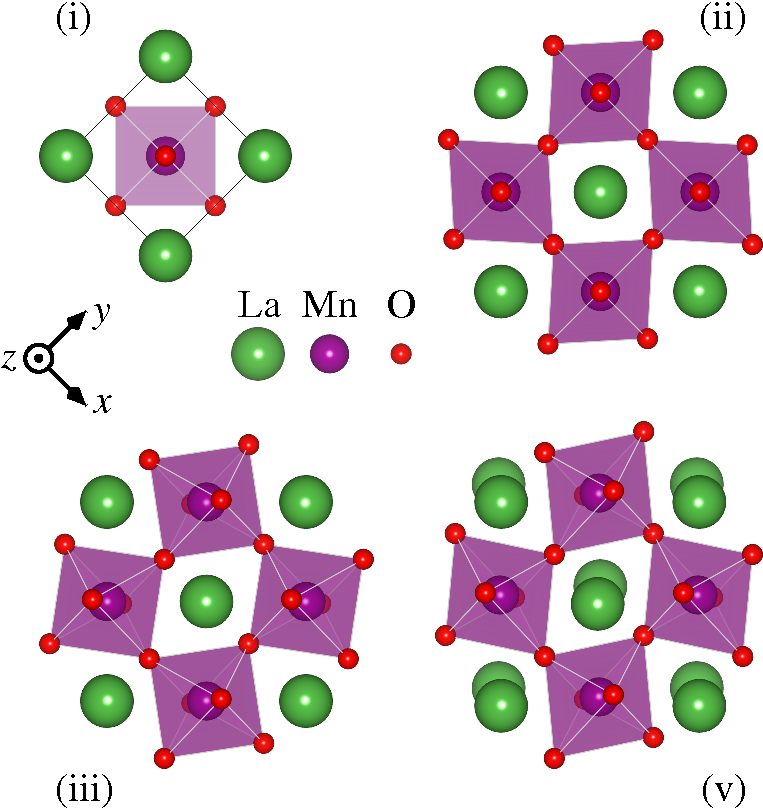
Figure 1: (Color online) Different structural modifications of LaMnO₃ investigated in this work, viewed along the [001] direction: (i) ideal cubic perovskite, (ii) purely Jahn-Teller distorted, (iii) purely GdFeO₃-type distorted, and (v) experimental $Pbnm$ structure. Pictures have been generated using VESTA.Momma and Izumi (2008)

LaMnO₃ crystallizes in an orthorhombically distorted perovskite structure with $Pbnm$ space group (see Fig. 1v), and A-type antiferromagnetic (A-AFM) order of the magnetic moments of the Mn cations.Wollan and Koehler (1955); Elemans et al. (1971) The deviation from the simple cubic perovskite structure (Fig. 1i) can be decomposed into a staggered JT distortion of the MnO₆ octahedra within the $x$-$y$ plane (Fig. 1ii), the so-called GdFeO₃-type (GFO) distortion, consisting of collective tiltings and rotations of the oxygen octahedra (Fig. 1iii), and “the rest”, i.e. displacements of the La cations from their ideal positions plus a homogeneous orthorhombic strain (Fig. 1v).Ederer et al. (2007)

The electronic structure of LaMnO₃ close to the Fermi energy is dominated by Mn 3$d$ states, which are split by the cubic component of the crystal field into the lower-lying three-fold degenerate $t_{2g}$ and the higher-lying two-fold degenerate $e_{g}$ states.Pickett and Singh (1996); Satpathy et al. (1996); Ederer et al. (2007) The formal electronic configuration Mn³⁺: [Ar] 3$d^{4}$ leads to a high spin state of the Mn cation with fully occupied local majority spin $t_{2g}$ states and one electron per local majority spin $e_{g}$ state, while both $t_{2g}$ and $e_{g}$ minority spin states are empty.

Based on this electronic structure, the theoretical description of manganites often employs an effective two-band TB picture, where electrons can hop between the two $e_{g}$ levels on each Mn site. This hopping is facilitated by hybridization with the oxygen 2$p$ states, which, however, are not explicitly included in the TB model. It is therefore understood, that the “atomic” $e_{g}$ states used in the TB model are indeed somewhat extended Wannier orbitals that also include the hybridization with the O 2$p$ states. In contrast, the three $t_{2g}$ electrons are assumed to be tightly bound to a specific Mn site where they give rise to a local “core spin” $S=3/2$. This core spin then interacts with the valence $e_{g}$ electron spin via Hund’s rule coupling. In addition, a JT distortion of the surrounding oxygen octahedron splits the two $e_{g}$ levels on the corresponding Mn site, whereas elastic coupling between neighboring oxygen octahedra gives rise to a cooperative effect. The GFO distortion in this picture is usually assumed to simply reduce the effective hopping amplitudes between neighboring Mn sites due to the resulting non-ideal Mn-O-Mn bond angle. In addition, a local electron-electron interaction between electrons occupying the same Mn site can be included in the model.Dagotto et al. (2001); Lin and Millis (2008)

The electronic Hamiltonian for such a model can be expressed as:

$$\hat{H}=\hat{H}_{\text{kin}}+\hat{H}_{\text{local}}\ ,$$ (1)

where

$$\hat{H}_{\text{kin}}=\sum_{a,b,\mathbf{R},\Delta\mathbf{R},\sigma}t_{ab}(\Delta\mathbf{R})\,\hat{c}^{\dagger}_{b(\mathbf{R}+\Delta\mathbf{R})\sigma}\hat{c}_{a\mathbf{R}\sigma}+\text{h.c.}$$ (2)

describes the electron hopping between orbital $|a\rangle$ (spin $\sigma$) at site $\mathbf{R}$ and orbital $|b\rangle$ at site $\mathbf{R}+\Delta\mathbf{R}$, and it is assumed that all sites are translationally equivalent, so that the hopping amplitudes $t_{ab}(\Delta\mathbf{R})$ depend only on the relative position between the two sites.

Representing the $e_{g}$ orbital subspace within the usual basis $|1\rangle=|3z^{2}-r^{2}\rangle$ and $|2\rangle=|x^{2}-y^{2}\rangle$, and assuming cubic symmetry, the nearest neighbor hopping along the three cartesian directions has the following form:

$$\mathbf{t}(\pm a_{\text{c}}\hat{\mathbf{z}}) =\left(\begin{matrix}t&0\\ 0&t^{\prime}\end{matrix}\right)$$ (3)

$$\mathbf{t}(\pm a_{\text{c}}\hat{\mathbf{x}}) =t\left(\begin{matrix}\tfrac{1}{4}&-\tfrac{\sqrt{3}}{4}\\ -\tfrac{\sqrt{3}}{4}&\tfrac{3}{4}\end{matrix}\right)+t^{\prime}\left(\begin{matrix}\tfrac{3}{4}&\tfrac{\sqrt{3}}{4}\\ \tfrac{\sqrt{3}}{4}&\tfrac{1}{4}\end{matrix}\right)$$ (4)

$$\mathbf{t}(\pm a_{\text{c}}\hat{\mathbf{y}}) =t\left(\begin{matrix}\tfrac{1}{4}&\tfrac{\sqrt{3}}{4}\\ \tfrac{\sqrt{3}}{4}&\tfrac{3}{4}\end{matrix}\right)+t^{\prime}\left(\begin{matrix}\tfrac{3}{4}&-\tfrac{\sqrt{3}}{4}\\ -\tfrac{\sqrt{3}}{4}&\tfrac{1}{4}\end{matrix}\right)\ .$$ (5)

Here, $a_{\text{c}}$ is the lattice constant of the underlying cubic perovskite structure. The hopping $t^{\prime}$ between two neighboring $|x^{2}-y^{2}\rangle$-type orbitals along $\hat{\mathbf{z}}$ is small due to the planar shape of this orbital, and it is therefore often neglected. In this case, the nearest neighbor hopping depends only on a single parameter $t$, the hopping along $\hat{\mathbf{z}}$ between $|3z^{2}-r^{2}\rangle$-type orbitals.

$\hat{H}_{\text{local}}$ contains all local interaction terms included in the model, i.e. Hund’s rule coupling with the $t_{2g}$ core spin, the JT coupling to the oxygen octahedra distortion, and eventually also the electron-electron interaction. In this work we will discuss only the Hund’s rule and JT coupling, which are of the form:

$$\hat{H}_{\text{Hund}}=-J\sum_{\mathbf{R}}\mathbf{S}_{\mathbf{R}}\cdot\mathbf{s}_{\mathbf{R}}\ ,\ \text{and}$$ (6)

$$\hat{H}_{\text{JT}}=-\lambda\sum_{\mathbf{R},\sigma,a,b}\left(Q^{x}_{\mathbf{R}}\hat{c}^{\dagger}_{a\mathbf{R}\sigma}\tau^{x}_{ab}\hat{c}_{b\mathbf{R}\sigma}+Q^{z}_{\mathbf{R}}\hat{c}^{\dagger}_{a\mathbf{R}\sigma}\tau^{z}_{ab}\hat{c}_{b\mathbf{R}\sigma}\right)\ .$$ (7)

Here, $J$ is the Hund’s rule coupling strength and $\mathbf{S}_{\mathbf{R}}$ is the $t_{2g}$ core spin at site $\mathbf{R}$, which in the following we will consider as classical vector normalized to $|\mathbf{S}_{\mathbf{R}}|=1$. $\mathbf{s}_{\mathbf{R}}=\sum_{a,\sigma,\sigma^{\prime}}c^{\dagger}_{a\mathbf{R}\sigma}\bm{\tau}_{\sigma\sigma^{\prime}}c_{a\mathbf{R}\sigma^{\prime}}$ is the corresponding $e_{g}$ valence spin, $\lambda$ describes the strength of the JT coupling, and $\bm{\tau}_{\sigma\sigma^{\prime}}$ are the usual Pauli matrices. The quantities $Q^{x}_{\mathbf{R}}$ and $Q^{z}_{\mathbf{R}}$ describe the JT distortion of the oxygen octahedron surrounding site $\mathbf{R}$:

$$Q^{x}_{\mathbf{R}}=\frac{1}{2\sqrt{2}}\left(d^{x}_{\mathbf{R}}-d^{y}_{\mathbf{R}}\right)\ ,$$ (8)

$$Q^{z}_{\mathbf{R}}=\frac{1}{2\sqrt{6}}\left(2d^{z}_{\mathbf{R}}-d^{x}_{\mathbf{R}}-d^{y}_{\mathbf{R}}\right)\ ,$$ (9)

where $d^{x}_{\mathbf{R}}$, $d^{y}_{\mathbf{R}}$, and $d^{z}_{\mathbf{R}}$ indicate the O-O distances along the $x$, $y$, and $z$ directions, corresponding to the oxygen octahedron located at site $\mathbf{R}$.

II.2 Maximally localized Wannier functions

As is well known from basic solid state physics, the eigenfunctions within a periodic crystal potential are extended Bloch waves, classified by a wave-vector $\mathbf{k}$ and a band-index $m$. These Bloch waves can in turn be expressed as a Bloch sum of “atomic-like” localized TB basis functions or Wannier functions. For an isolated group of $N$ Bloch states $\lvert\psi_{m\mathbf{k}}\rangle$, i.e. a group of bands that are energetically separated from all lower- or higher-lying bands throughout the entire Brillouin zone (BZ), a set of $N$ localized Wannier functions $\lvert w_{n\mathbf{T}}\rangle$, associated with lattice vector $\mathbf{T}$, is defined via the following transformation:Marzari and Vanderbilt (1997); Souza et al. (2001)

$$\lvert{w_{n\mathbf{T}}}\rangle=\frac{V}{\left({2\pi}\right)^{3}}\int_{\mathrm{BZ}}\left[{\sum_{m=1}^{N}U_{mn}^{\left(\mathbf{k}\right)}\lvert{\psi_{m\mathbf{k}}}\rangle}\right]\mathrm{e}^{-\mathrm{i}\mathbf{k}\cdot\mathbf{T}}\,\mathrm{d}\mathbf{k}\,.$$ (10)

Here, $\mathbf{U}^{\left({\mathbf{k}}\right)}$ is a unitary matrix mixing Bloch states at wave-vector $\mathbf{k}$. Different $\mathbf{U}^{\left({\mathbf{k}}\right)}$ lead to different Wannier orbitals, which are not uniquely determined by Eq. (10). However, Marzari and Vanderbilt showed that a unique set of maximally localized Wannier functions (MLWFs) can be obtained by minimizing the total quadratic spread of the Wannier orbitals, defined as:Marzari and Vanderbilt (1997)

$$\Omega=\sum_{n}^{N}\left[{\langle{r^{2}}\rangle_{n}-\langle\mathbf{r}\rangle_{n}^{2}}\right]\,,$$ (11)

where $\langle\hat{O}\rangle_{n}=\langle w_{n\mathbf{0}}|\hat{O}|w_{n\mathbf{0}}\rangle$.

For the case of entangled Bloch bands, i.e. bands that are not energetically separated from other groups of higher- or lower-lying states, an energy window $[E_{\text{min}},E_{\text{max}}]$ can be defined such that there are $N_{\mathrm{win}}^{\left({\mathbf{k}}\right)}>N$ Bloch bands within the energy window at each $\mathbf{k}$ vector, and then an $N$-dimensional manifold of mixed Bloch states is obtained as:Souza et al. (2001)

$$\lvert\psi_{m\mathbf{k}}^{\mathrm{dis}}\rangle=\sum_{l\in N_{\mathrm{win}}^{\left({\mathbf{k}}\right)}}U_{lm}^{\mathrm{dis}\left(\mathbf{k}\right)}\lvert{\psi_{l\mathbf{k}}}\rangle\,.$$ (12)

The corresponding Wannier functions can then be obtained from the mixed Bloch states by replacing $\lvert\psi_{m\mathbf{k}}\rangle$ with $\lvert\psi_{m\mathbf{k}}^{\mathrm{dis}}\rangle$ in Eq. (10). The unitary rectangular $N_{\mathrm{win}}^{\left({\mathbf{k}}\right)}\times N$ matrix $\mathbf{U}^{\mathrm{dis}\left(\mathbf{k}\right)}$ is also uniquely determined by the condition of maximal localization, i.e. it can be obtained by minimizing $\Omega\left(\mathbf{U}^{\left(\mathbf{k}\right)},\mathbf{U}^{\mathrm{dis}\left(\mathbf{k}\right)}\right)$.Souza et al. (2001)

Once a set of MLWFs is obtained, the corresponding Hamilton matrix, $\mathbf{H}^{\left(\mathrm{W}\right)}\left(\mathbf{k}\right)$, is constructed by a unitary transformation:

$$\mathbf{H}^{\left(\mathrm{W}\right)}\left(\mathbf{k}\right)=\bigl{(}\mathbf{U}^{(\mathbf{k})}\bigr{)}^{\dagger}\bigl{(}\mathbf{U}^{\mathrm{dis}(\mathbf{k})}\bigr{)}^{\dagger}\mathbf{H}^{(\text{B})}\left(\mathbf{k}\right)\mathbf{U}^{\mathrm{dis}(\mathbf{k})}\mathbf{U}^{(\mathbf{k})}\,,$$ (13)

from the (diagonal) Hamilton matrix in the Bloch basis, $H^{(\text{B})}_{nm}\left(\mathbf{k}\right)=\varepsilon_{n\mathbf{k}}\delta_{nm}$, with eigenvalues $\varepsilon_{n\mathbf{k}}$. The MLWF Hamiltonian in real space is then calculated as a Fourier transform of $\mathbf{H}^{\left(\mathrm{W}\right)}\left(\mathbf{k}\right)$, which in practice is replaced by a sum over $N_{k}$ points in $\mathbf{k}$-space:

$$h^{\mathbf{T}}_{nm}=\frac{1}{N_{k}}\sum_{\mathbf{k}}\mathrm{e}^{-\mathrm{i}\mathbf{k}\cdot\mathbf{T}}H_{nm}^{(\text{W})}\left(\mathbf{k}\right)\,.$$ (14)

Thus, the real space representation of the Hamiltonian in the MLWF basis is equivalent to a TB description of the full Hamiltonian within the corresponding orbital subspace:

$$\hat{H}=\sum_{\mathbf{T},\Delta\mathbf{T}}h_{nm}^{\Delta\mathbf{T}}\,\hat{c}^{\dagger}_{n\mathbf{T}+\Delta\mathbf{T}}\hat{c}_{m\mathbf{T}}\ +\text{h.c.}\ ,$$ (15)

where $c_{m\mathbf{T}}$ is the annihilation operator for an electron in orbital $\lvert w_{m\mathbf{T}}\rangle$. The real space MLWF matrix elements $h_{nm}^{\mathbf{T}}$ can therefore be interpreted as hopping amplitudes within a TB picture of MLWFs [compare Eq. (15) with Eq. (2)]. Note that $\Delta\mathbf{T}$ in Eq. (15) refers to lattice vectors, whereas $\Delta\mathbf{R}$ in Eq. (2) refers to Mn sites. The subscripts $n$ and $m$ in Eq. (15) can thus in general indicate both site and orbital/spin character (for cases with more than one site per unit cell).

For the case when MLWFs are constructed from an isolated set of bands, the TB model, Eq. (15), exactly reproduces the band dispersion within the corresponding energy window. For the entangled case, the energy bands calculated from Eq. (15) do not necessarily have to coincide with the underlying Bloch bands.

II.3 Structural decomposition

To analyze the effect of the various distinct structural distortions within the experimental $Pbnm$ structure on the electronic properties of LaMnO₃ we investigate several different atomic configurations (similar to Ref. Ederer et al., 2007):

1. The ideal cubic perovskite structure (Fig. 1i).

2. A purely JT distorted structure (Fig. 1ii), which results from alternating long and short O-O distances within the $x$-$y$ plane, i.e. a staggered JT distortion $Q^{x}_{\mathbf{R}}=\pm Q^{x}_{\mathbf{0}}$ and $Q^{z}_{\mathbf{R}}=0$. This distortion doubles the unit cell within the $x$-$y$ plane, leading to new in-plane lattice vectors $\mathbf{a}_{\mathrm{ii}}=a_{\mathrm{c}}(\mathbf{\hat{y}}+\mathbf{\hat{x}})$ and $\mathbf{b}_{\mathrm{ii}}=a_{\mathrm{c}}(\mathbf{\hat{y}}-\mathbf{\hat{x}})$ and tetragonal symmetry.

3. A purely GFO-distorted structure (Fig. 1iii), resulting from rotations of the oxygen octahedra around the $z$ direction and octahedral tilts away from $z$, alternating along all three cartesian directions. This distortion quadruples the unit cell compared to the undistorted structure (i), yielding orthorhombic $Pbnm$ symmetry. The resulting in-plane lattice vectors are identical to those of structure (ii) and the new lattice vector along $z$ is $\mathbf{c}_{\mathrm{iii}}=2a_{\mathrm{c}}\hat{\mathbf{z}}$.

4. A superposition of JT and GFO distortion, which also leads to orthorhombic $Pbnm$ symmetry and unit cell vectors unchanged with respect to structure (iii).

5. The full experimental structure (Fig. 1v), with orthorhombically strained lattice vectors ($|\mathbf{a}_{\mathrm{v}}|\neq|\mathbf{b}_{\mathrm{v}}|\neq|\mathbf{c}_{\mathrm{v}}|$, resulting in $Q^{z}_{\mathbf{R}}\neq 0$) and displaced La cations compared to structure (iv).

For each of these structural modifications we use the same volume $V=60.91$ Å³ per formula unit as in the experimentally observed $Pbnm$ structure.Norby et al. (1995) This leads to a cubic lattice parameter $a_{\text{c}}=3.9345$ Å, which deviates only by 0.8$\,\%$ from the value we obtain by volume optimization for the ideal perovskite structure within GGA. For the positions of the O anions in structures (ii) and (iii) we use the same decomposition of structure (iv) into pure JT and GFO components as described in Ref. Ederer et al., 2007 (see Table 1). For the cases with A-AFM order, the unit cell is doubled in $z$ direction for both (i) and (ii) structures in order to accommodate the magnetic order, thus changing the symmetry to tetragonal in case (i).

Table 1: Wyckoff parameters of the O(4c), ($x$, $y$, 0.25), O(8d), ($x$, $y$, $z$), and La(4c), ($x$, $y$, 0.25), sites for the various structural configurations used in this work (compare with Table I in Ref. Ederer et al., 2007).

		Expt. (Ref. Norby et al., 1995)	(ii)	(iii)	(iv)	(v)
O(4c)	$x$	-0.0733	0.0	-0.0733	-0.0733	-0.0733
	$y$	-0.0107	0.0	-0.0107	-0.0107	-0.0107
O(8d)	$x$	0.2257	0.2636	0.2121	0.2257	0.2257
	$y$	0.3014	0.2636	0.2879	0.3014	0.3014
	$z$	0.0385	0.0	0.0385	0.0385	0.0385
La(4c)	$x$	0.0063	0.0	0.0	0.0	0.0063
	$y$	0.5436	0.5	0.5	0.5	0.5435

Starting from the ideal cubic perovskite structure, we analyze the effect of a specific distortion by gradually increasing the amount of this distortion, i.e. we perform series of calculations using a linear superposition of the Wyckoff positions in the cubic perovskite structure and in structure $(x)$:

$$\mathbf{R}(\alpha_{x})=(1-\alpha_{x})\,\mathbf{R}^{(\mathrm{i})}+\alpha_{x}\,\mathbf{R}^{(x)}\,,$$ (16)

and vary $\alpha_{x}$ between 0 and 1. The following cases are considered: ($x=$ii) (pure JT distortion), ($x=$iii) (pure GFO distortion), ($x=$iv) (combined JT and GFO distortions).

II.4 Computational details

We perform spin-polarized first principles DFT calculations using the Quantum-ESPRESSO program package, qua the GGA exchange-correlation functional of Perdew, Burke, and Ernzerhof,Perdew et al. (1996) and Vanderbilt ultrasoft pseudopotentials Vanderbilt (1990) in which the La (5$s$,5$p$) and Mn (3$s$,3$p$) semicore states are included in the valence.

Convergence has been tested for the total energy and total magnetization using the ideal cubic perovskite structure and ferromagnetic (FM) order. We find the total energy converged to an accuracy better than 1 mRy and the total magnetization converged to an accuracy of 0.05 $\mu_{\mathrm{B}}$ for a a plane-wave energy cut-off of 35 Ry and a $\Gamma$-centered ${10}\!\times\!{10}\!\times\!{10}$ k-point grid using a Gaussian broadening of 0.01 Ry. These values for plane-wave cutoff and Gaussian broadening are used in all calculations presented in this work. The ${10}\!\times\!{10}\!\times\!{10}$ k-point grid is used in all calculations for the cubic structure (i), whereas appropriately reduced k-point grids of ${10}\!\times\!{10}\!\times\!{5}$, ${7}\!\times\!{7}\!\times\!{10}$, and ${7}\!\times\!{7}\!\times\!{5}$ are used for the structures with unit cell doubled in the $z$ direction, doubled in the $x$-$y$ plane, and quadrupled, respectively.

After obtaining the DFT Bloch bands within GGA, we construct MLWFs using the wannier90 program integrated into the Quantum-ESPRESSO package. Mostofi et al. (2008) Starting from an initial projection of the Bloch bands onto atomic $d$ basis functions $\lvert{3z^{2}-r^{2}}\rangle$ and $\lvert{x^{2}-y^{2}}\rangle$ centered at the different Mn sites within the unit cell, we obtain a set of two $e_{g}$-like MLWFs per spin channel for each site. The spread functional (both gauge-invariant and non-gauge-invariant parts) is considered to be converged if the corresponding fractional change between two successive iterations is smaller than $10^{-10}$. For cases with entangled bands a suitable energy window is chosen as described in the corresponding “Results” section.

III Results and Discussion

III.1 Perfect cubic perovskite – structure (i)

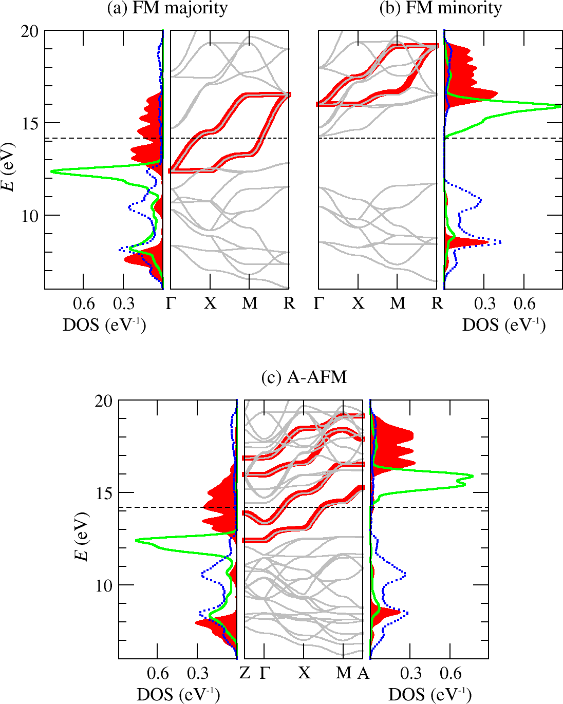
Figure 2: (Color online) Projected DOS and band structure along high symmetry lines within the BZ calculated for the cubic structure (i) and both FM and A-AFM order. Filled (red) areas and solid (green) lines represent the projected DOS corresponding to Mn($e_{g}$) and Mn($t_{2g}$) states, respectively, while dashed (blue) lines represent the site and orbitally averaged projected DOS corresponding to the O $p$ states. For the A-AFM case the left (right) panel corresponds to local majority (minority) spin projection. In the band structure plots, the dispersion calculated from the $e_{g}$-like MLWFs are represented by thick (red) lines. The Fermi level is indicated by the horizontal dashed lines.

The projected densities of states (DOS) and band structure calculated for LaMnO₃ in the ideal cubic perovskite structure (i) for both FM and A-AFM order are shown in Fig. 2.foo (a)

A metallic state is obtained for both FM and A-AFM order, in agreement with previous band-structure calculations.Pickett and Singh (1996); Satpathy et al. (1996); Ederer et al. (2007) The projected DOS show that the (local) majority spin bands around the Fermi energy have mainly Mn($e_{g}$) character and are half-filled while the (local) minority spin bands with mainly Mn($e_{g}$) character are unoccupied, as expected from the formal electron configuration. Bands with Mn($t_{2g}$) character are lying just below the Mn($e_{g}$) bands, and slightly overlap with the latter. O($p$) bands are located below the Mn($t_{2g}$) bands (between $\sim$ 6-12 eV) and are fully occupied. The strong hybridization between Mn($d$) and O($p$) electrons can be seen from the substantial amount of Mn($d$) character in the energy range around 8 eV, i.e. towards the bottom of the bands with predominant O($p$) character. The states above the Mn($e_{g}$) bands have predominantly La($d$) character.

One can see from the band structures depicted in Fig. 2 that for the FM majority spin channel the bands with predominant $e_{g}$ character are nearly completely isolated from both higher and lower-lying bands, while for the FM minority spin channel and in the A-AFM case, the “$e_{g}$ bands” overlap strongly with other bands (with mostly Mn($t_{2g}$) minority and La($d$) character). As described in section II.4, in order to construct $e_{g}$-like MLWFs for the various cases, we define an energy window for the disentanglement procedure [see Eq. (12)], and then initialize the Wannier functions from a projection of the Kohn-Sham states within that energy window on atomic $e_{g}$ wave-functions (see Ref. Souza et al., 2001). A suitable energy window is chosen based on the $e_{g}$ projected DOS and calculated band structure (see discussion below for more details). Two MLWFs per spin channel for the single Mn site within the cubic unit cell are constructed for FM order, and two pairs of MLWFs, localized at the two Mn sites within the magnetic unit cell, are constructed for A-AFM order (for global spin up projection only).

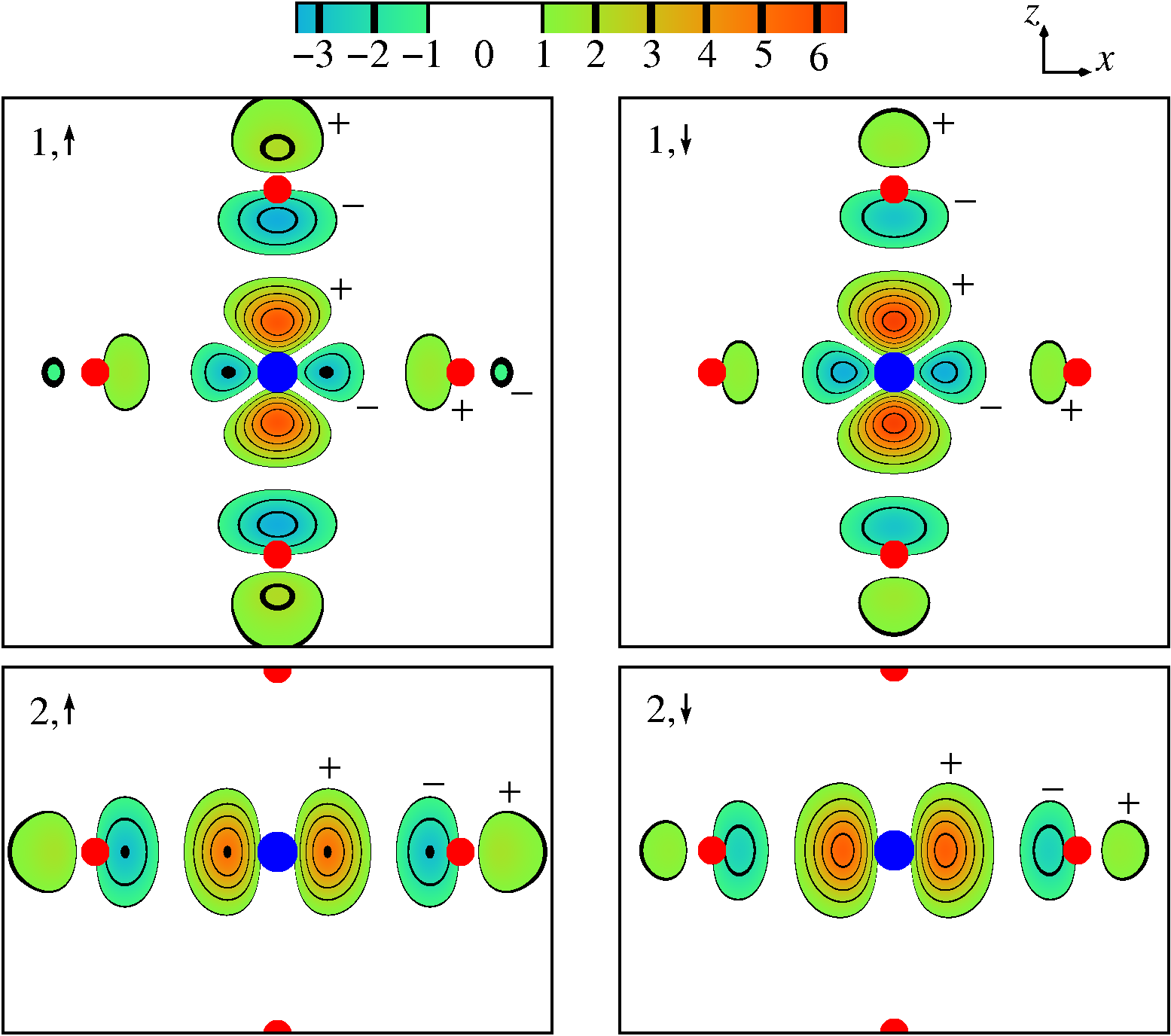
Figure 3: (Color online) Real space representation of the MLWFs for majority and minority spin projections in the cubic structure (i) with FM order, projected on the $x$-$z$ plane passing through Mn (large/blue sphere) and O (small/red spheres) sites (in arbitrary units).

Figure 3 shows the real space representation of the two $e_{g}$-like MLWFs for both majority and minority spin and FM order, calculated for an energy window of [12.0, 17.0] eV and [15.9, 20.0] eV, respectively. The shape of the MLWFs resembles the antibonding $\sigma^{*}$ character of hybridization between Mn($e_{g}$) and O($p$) states in this energy range. The hybridization is notably stronger for the majority spin MLWFs (individual spread per WF $2.90$ $\mathrm{\AA^{2}}$ compared to $1.65$ $\mathrm{\AA^{2}}$ for the minority spin MLWFs), which is due to the smaller energy separation between the atomic Mn($e_{g}$) and O($p$) levels for the majority spin channel. The difference between the real space representation of the MLWFs for FM and A-AFM order (not shown here) is more subtle. A quantitative comparison of the corresponding differences in the real space Hamilton matrix elements between MLWFs will be presented below.

The dispersion calculated from the obtained $e_{g}$ MLWFs is also shown in Fig. 2. It can be seen that even in the cases with strongly entangled $e_{g}$ bands (FM minority spin and A-AFM) the MLWF bands follow certain DFT bands almost exactly, except around some band crossings with higher lying La $d$ bands. This represents the fact that within cubic symmetry the $e_{g}$ states cannot hybridize with the $t_{2g}$ bands, and hybridize only very weakly with the La $d$ states.

In order to reproduce the two majority spin bands around the Fermi energy for the FM case, the lower bound of the energy window, $E_{\text{min}}$, has to be above the lower peaks in the Mn($e_{g}$) projected DOS at around 10.5 eV and 8 eV, which correspond to the bonding combination of hybridized atomic O($p$) and Mn($e_{g}$) states. If these bands are included in the energy window, the bonding and antibonding combinations of atomic orbitals become disentangled and the $e_{g}$ Wannier functions become essentially “atomic-like” (compare also with the case of SrVO₃ described in Ref. Lechermann et al., 2006). On the other hand, varying $E_{\text{min}}$ within 0.4 eV below the $\Gamma$ point energy of the $e_{g}$-like bands changes the MLWF bands by less than 1 meV for any $\mathbf{k}$. Similarly, varying the upper bound of the energy window has only minor influence on the resulting MLWF bands, due to the negligible hybridization of the $e_{g}$ states with higher-lying bands. Additional test calculations for different k-point grids showed that the MLWF band structure is converged within 0.5 meV at any k-point for the ${10}\!\times\!{10}\!\times\!{10}$ grid which was used for the energy window test calculations.

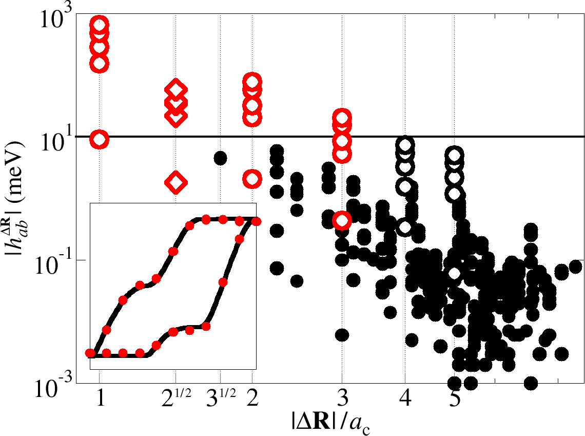
Figure 4: (Color online) Magnitude of all calculated non-zero hopping parameters for FM order in the ideal cubic structure as a function of the inter-site distance $|\Delta\mathbf{R}|$ (open circles: hopping along the unit cell directions; open diamonds: hopping between next-nearest neighbors; filled circles: all other hoppings). Inset: Comparison of the full MLWF band structure (solid lines) and the one calculated from a simplified TB model (filled circles) which includes only the inter-site hoppings for which the largest matrix element is larger than 10 meV (see main text).

We now turn to the analysis of the hopping parameters, i.e. the real space matrix elements $h_{ab}^{\Delta\mathbf{R}}$, Eq. (14), between MLWFs located at different Mn sites. The magnitudes of all calculated hopping parameters for the FM majority spin case are shown in Fig. 4. It is noticeable that the hopping amplitudes along the three cartesian axes are most dominant and that their decay with distance is rather slow, so that the terms corresponding to inter-site distances of $2a_{\mathrm{c}}$ and $3a_{\mathrm{c}}$ are of comparable magnitude as the hopping between next-nearest neighbors for which $\lvert\Delta\mathbf{R}\rvert=\sqrt{2}a_{\mathrm{c}}$.

The exact MLWF representation in terms of $\mathbf{H}^{(\text{W})}(\mathbf{k})$ is well suited for further numerical calculations, e.g. within a DFT+DMFT approach. On the other hand, for the analysis of specific physical mechanisms within a semi-analytical TB model, one generally wants to use only a very limited number of hopping parameters $\mathbf{h}^{\Delta\mathbf{R}}$ between closest neighbors. We therefore identify a minimal subset of hopping parameters, corresponding to intersite distances $\lvert\Delta\mathbf{R}\rvert/a_{\mathrm{c}}\in\{1,\sqrt{2},2,3\}$, i.e. where only hopping between sites, for which the leading term (i.e. the corresponding matrix element with largest magnitude) is larger than 10 meV, are considered, while the rest is set to zero. This model yields an overall very good agreement with the full MLWF band structure (see inset in Fig. 4), deviating not more than 0.11 eV for any k-point on the ${10}\!\times\!{10}\!\times\!{10}$ k-point grid used. On the other hand, a TB model where only the hopping amplitudes between nearest and next-nearest neighbors are taken into account leads to deviations of up to 0.29 eV for some k-points, which might still be acceptable for certain purposes. However, the overall bandwidth for the latter model is reduced by about 0.2 eV compared to the full MLWF band structure.

Table 2: Calculated values of the on-site, nearest, and next-nearest neighbor matrix elements $h_{ab}^{\Delta\mathbf{R}}$ (in meV) for FM and A-AFM order within structure (i) for the two different spin projections. As described in the text, in the A-AFM case all matrix elements refer to the Mn site closest to the origin.

(a)	FM($\uparrow$)	FM($\downarrow$)	A-AFM($\uparrow$)	A-AFM($\downarrow$)
$h_{11}^{0}$	$14485.7$	$17483.9$	$14638.9$	$17379.3$
$h_{22}^{0}$	$14484.3$	$17483.7$	$14541.7$	$17443.3$
$h_{11}^{z}$	$-648.2$	$-512.5$	$-595.0$
$h_{22}^{z}$	$9.1$	$-9.2$	$-8.5$
$h_{11}^{x}$	$-155.2$	$-135.0$	$-172.8$	$-130.7$
$h_{12}^{x}$	$284.5$	$217.9$	$281.4$	$214.5$
$h_{22}^{x}$	$-483.9$	$-386.7$	$-488.8$	$-389.8$
$h_{11}^{xz}$	$37.8$	$32.0$	$34.7$
$h_{12}^{xz}$	$-34.1$	$-26.6$	$-29.3$	$-29.0$
$h_{22}^{xz}$	$-1.8$	$1.2$	$0.5$
$h_{11}^{xy}$	$-21.9$	$-14.3$	$-16.4$	$-14.2$
$h_{22}^{xy}$	$57.9$	$47.4$	$51.4$	$48.3$

The calculated matrix elements of the real space matrix elements $h_{ab}^{\Delta\mathbf{R}}$ for nearest and next nearest neighbor hopping as well as the corresponding on-site terms ($\Delta\mathbf{R}=0$) are summarized in Table 2. Here and in the following we use the abbreviated notation $\mathbf{h}^{z}$, corresponding to $\Delta\mathbf{R}=\pm a_{\text{c}}\hat{\mathbf{z}}$, and $\mathbf{h}^{xz}$, corresponding to $\Delta\mathbf{R}=a_{\text{c}}(\pm\hat{\mathbf{x}}\pm\hat{\mathbf{z}})$ (and analogously for all other cartesian directions). We note that in the A-AFM case the translational equivalence between the two Mn sites within the unit cell is broken, and $\Delta\mathbf{R}=\pm a_{\text{c}}\hat{\mathbf{z}}$ is not a lattice vector in this case. Nevertheless, in order to simplify the notation, we stick to the site-based index and note that for A-AFM order a translation along $\hat{\mathbf{z}}$ is equivalent to reversing the two spin projections. In the following we always report hopping amplitudes corresponding to hopping from and to the Mn site at the origin, the corresponding parameters for all other sites within the unit cell follow from symmetry. Similarly, we do not add a spin index to the MLWF matrix elements but instead discuss each case separately.

It can be seen that the hopping parameter between two $\lvert{3z^{2}-r^{2}}\rangle$-like MLWFs along the $z$ direction, $h_{11}^{z}$ ($\equiv t$ in the effective model description), is the leading term for the nearest neighbor hopping, and that overall the next nearest neighbor hopping is about an order of magnitude smaller than the nearest neighbor hopping. The hopping amplitude between two $\lvert{x^{2}-y^{2}}\rangle$-like functions along the $z$ direction, $h^{z}_{22}$ ($\equiv t^{\prime}$ in the model description), is indeed very small compared to $h^{z}_{11}$. In the FM case, all nearest neighbor hopping amplitudes for the minority spin orbitals (except $h^{z}_{22}$) are reduced (to about 75-85%) compared to the majority spin channel. This reflects the weaker hybridization between minority spin $e_{g}$ and O(2$p$) states, leading to more localized minority spin MLWFs with reduced hopping amplitudes. For A-AFM order, $h_{11}^{z}$ corresponds to the hopping between a local majority and a local minority spin orbital, and its value, (92 % of $h_{11}^{z}$ for FM ($\uparrow$)), is intermediate between the corresponding FM majority and minority values. The A-AFM hopping amplitudes within ferromagnetically ordered $x$-$y$ planes for local majority/minority spin directions are very similar to the corresponding FM hoppings (differing by less than 5 meV), with the exception of the (local) majority spin $h_{11}^{x}$ value, which is larger than that. Similar relations between the FM majority and minority spin and A-AFM values are also observed for the next-nearest neighbor hoppings.

It can easily be verified, that the hopping parameters for FM majority and minority spin fulfill the relations described in Eqs. (3)-(5), as required for cubic symmetry. However, if the terms proportional to $t^{\prime}\equiv h^{z}_{22}$ are neglected, the corresponding equations are not exactly fulfilled. Thus, simply neglecting $h^{z}_{22}$ while keeping all other nearest neighbor hopping amplitudes unchanged, leads to slight deviations from cubic symmetry. Furthermore, Eqs. (3)-(5) are clearly not fulfilled for the A-AFM hopping amplitudes, which reflects the overall tetragonal symmetry resulting from the magnetic order.

This symmetry reduction for the A-AFM case is also visible in the on-site matrix elements $h^{0}_{11}$ and $h^{0}_{22}$, which differ by about 100 meV. On the other hand, the small asymmetry ($\sim$ 1 meV) in these on-site terms for FM order results from small numerical accuracies during the total spread minimization (which uses the full k-point grid, so that cubic symmetry is not automatically enforced).

Within the effective two-band model for manganites described in Sec. II.1, the Hund’s rule coupling leads to an on-site spin splitting equal to $2J$ (treating $\mathbf{S}_{\mathbf{R}}$ as classical unit vector). From the calculated on-site MLWF matrix elements, we thus obtain a value of $J=1.499$ eV for the Hund’s rule coupling parameter in the FM case, and $J=1.370/1.451$ eV from the A-AFM on-site terms. The differences between these values indicate the limits of the assumption of a fixed $t_{2g}$ core spin. We note that all these values are slightly larger than the results obtained in previous LSDA calculations ($J=1.34$ eV),Ederer et al. (2007) which reflects the fact that GGA in general leads to a stronger magnetic splitting than LSDA.Singh and Ashkenazi (1992); Lechermann et al. (2002)

Overall, the results obtained via MLWFs are in a very good qualitative agreement with the previous study using TB fits to DFT band structures.Ederer et al. (2007) However, the direct comparison between the values calculated from MLWF in this work and the values reported in Ref. Ederer et al., 2007 is slightly hampered by the different exchange correlation functionals and pseudopotentials used in the two studies. The same fitting method as described in Ref. Ederer et al., 2007 applied to the GGA band structure calculated in the present work, leads to a nearest neighbor hopping parameter $t=-688$ meV, i.e. slightly larger than the $-$648 meV obtained from the MLWFs. This is due to the larger majority spin $e_{g}$ bandwidth obtained here, $W_{\uparrow}=4.126$ eV, compared to the value of 3.928 eV reported in Ref. Ederer et al., 2007. Thus, the difference in bandwidth compensates the neglect of further neighbor hopping in the simple TB fit, leading to the apparent very good agreement between $h^{z}_{11}=-648$ meV listed in Table 2 and the corresponding value ($t=-655$ meV) given in Ref. Ederer et al., 2007.

In the following sections, we will analyze the influence of the structural distortions only for the on-site and nearest-neighbor hopping terms. We have verified that the resulting changes in the further neighbor hopping amplitudes do not lead to significant differences in the dispersion characteristics of the $e_{g}$ bands, even though the corresponding relative changes of the next-nearest neighbor hoppings are comparable with those of the nearest-neighbor hoppings.

III.2 Jahn-Teller distortion – structure (ii)

As described in Sec. II.3, the staggered JT distortion, $Q^{x}_{\mathbf{R}}=\pm Q^{x}_{\mathbf{0}}$, leads to a unit cell doubling within the $x$-$y$ plane. In the case of FM order, we therefore construct two pairs of $e_{g}$ MLWFs for each spin channel, localized at the two different Mn sites within the unit cell, while for A-AFM order we construct four pairs of MLWFs, localized at the four different Mn sites within the corresponding unit cell (for global spin up projection only). The same approach for choosing the energy window for the disentanglement procedure was used as described in the previous section.

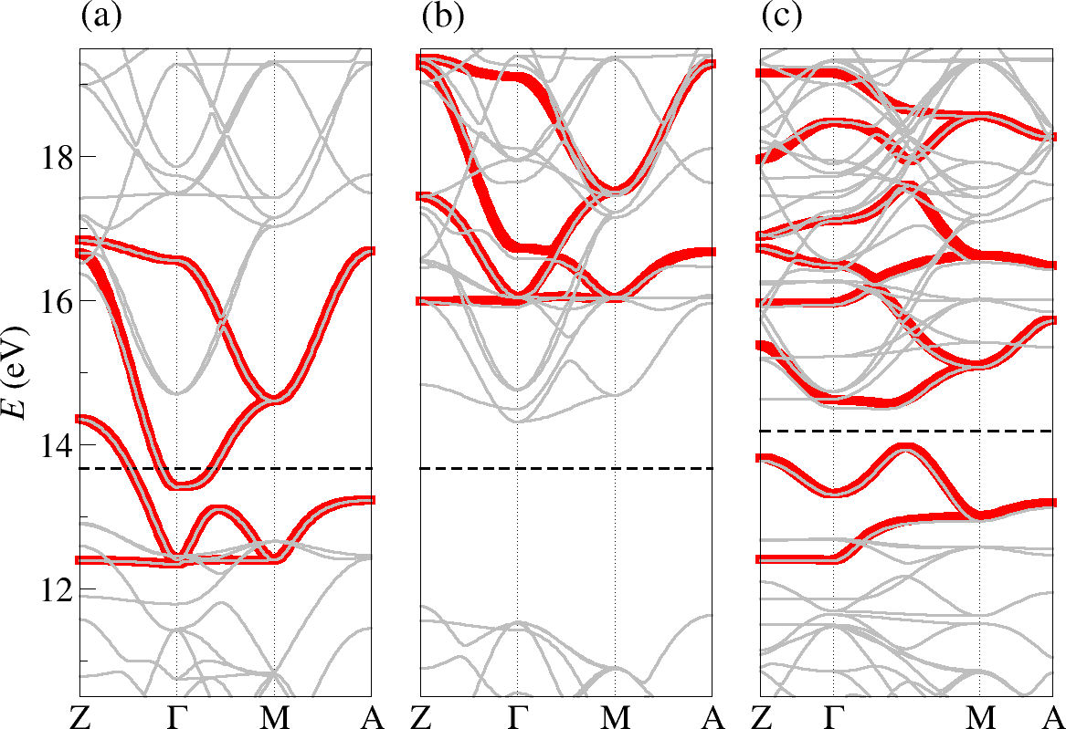
Figure 5: (Color online) DFT band structure (thin lines) for the JT-distorted structure (ii): a) majority spin FM, b) minority spin FM, and c) A-AFM. MLWF bands are depicted as thick/red lines. The Fermi level is indicated by the dashed line.

The calculated DFT band structure and $e_{g}$-like MLWF dispersion for the JT distorted structure (ii) are shown in Fig. 5. As a result of the unit cell doubling, there are now 4 and 8 bands with $e_{g}$ character per spin channel for the FM and A-AFM order, respectively. As for the cubic perovskite structure, the calculated MLWF dispersion largely follows the DFT band structure, except where there is strong hybridization with states of a different orbital character. It can be seen that several degeneracies and potential band crossings, which would result from a simple “backfolding” of the cubic band-structure onto the smaller tetragonal BZ, are lifted due to the JT distortion. This can be seen for example for the FM majority spin bands, where the highest-lying band along $\Gamma\mathrm{Z}$ acquires some dispersion, leading to a splitting of the higher energy $e_{g}$ states at Z. Similarly, the degeneracy of the two lowest-lying $e_{g}$ states at $\Gamma$ is lifted, and a potential crossing of $e_{g}$ bands is prevented between $\Gamma$ and M. The latter splitting, together with the reduced dispersion along $\Gamma\mathrm{Z}$ for A-AFM order, appears crucial for the opening of an energy gap in the JT-distorted A-AFM ordered structure (Fig. 5c).

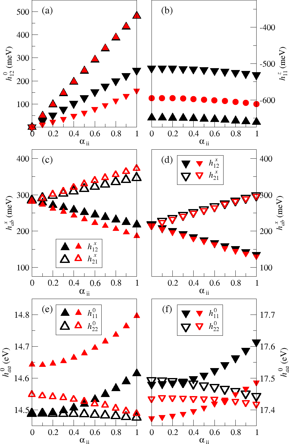
Figure 6: (Color online) MLWF Hamiltonian matrix elements $h^{\Delta\mathbf{R}}_{ab}$ as function of the JT distortion. Large/black and small/red symbols correspond to FM and A-AFM order, respectively. Matrix elements associated with pure (local) majority and minority spin character are shown as triangles pointing up and down, respectively. Closed circles in (b) represent the A-AFM $h_{11}^{z}$ hopping.

To further analyze the influence of the JT distortion on the $e_{g}$ electronic structure, we perform a series of calculations where we gradually change the oxygen positions from the ideal perovskite structure (i) to the fully JT distorted structure (ii), according to Eq. (16), and monitor the resulting changes in the MLWF Hamiltonian matrix elements. In all these calculations, we use the same energy windows of $[12.0,17.5]$ eV, $[15.9,20.0]$ eV and $[12.0,20.0]$ eV for the disentanglement in the case of FM majority, FM minority and A-AFM, respectively. The resulting MLWF matrix elements are depicted in Fig. 6. As discussed in the previous section, we report only hopping from and to the Mn site at the origin. The hopping amplitudes corresponding to other sites in the unit cell follow from symmetry. We find a strong linear dependence on the JT distortion for both the off-diagonal on-site matrix elements $h^{0}_{12}$ (Fig. 6a) as well as for the off-diagonal in-plane hopping $h^{x}_{12/21}$ (Fig. 6c/d). All other on-site and nearest neighbor hopping matrix elements show only a weak or moderate quadratic dependence on $\alpha_{\mathrm{ii}}$.

Within the model described in Sec. II.1 the sole effect of the JT distortion $(Q^{x}_{\mathbf{R}},Q^{z}_{\mathbf{R}})$ is a linear coupling to the on-site terms at site $\mathbf{R}$ according to:

$$\mathbf{t}^{0}=\left(\begin{array}[]{cc}e_{0}-\lambda Q^{z}_{\mathbf{R}}&-\lambda Q^{x}_{\mathbf{R}}\\ -\lambda Q^{x}_{\mathbf{R}}&e_{0}+\lambda Q^{z}_{\mathbf{R}}\end{array}\right)\ .$$ (17)

In our case $Q^{z}_{\mathbf{R}}=0$ and $Q^{x}_{\mathbf{R}}=\pm\alpha_{\mathrm{ii}}Q^{x}_{\mathbf{0}}$; $e_{0}$ is the on-site energy of the $e_{g}$ orbitals. It can be seen from Fig. 6a that the off-diagonal element $h^{0}_{12}$ indeed shows a linear dependence on $\alpha$, consistent with Eq. (17). The corresponding slope, $-\lambda Q^{x}_{\mathbf{0}}=482$ meV, is nearly identical for the FM majority and A-AFM local majority spin elements, whereas it is significantly smaller for the (local) minority spin matrix elements ($-\lambda Q^{x}_{\mathbf{0}}=246/155$ meV). This indicates that the JT splitting is also a ligand-field effect, i.e. it is mediated by hybridization with the surrounding oxygen orbitals, which, as pointed out previously, is stronger for the energetically lower majority spin states. The values for the JT coupling constant $\lambda$ obtained from the data shown in Fig. 6a are 3.19 eV/Å, 1.63 eV/Å, and 1.02 eV/Å, for majority, FM minority, and A-AFM local minority spin states, respectively. We note that the value of $\lambda$ obtained for majority spin is approximately a factor of two larger than the value obtained from the fitting procedure described in Ref. Ederer et al., 2007. As we will discuss in more detail below, the source for this discrepancy is the strong linear splitting observed for the off-diagonal in-plane nearest neighbor hoppings $h^{x}_{12/21}$, which is induced by the JT distortion (see Fig. 6c/d).

This splitting between $h^{x}_{12/21}$ again results from the underlying hopping between atomic Mn($e_{g}$) and O($p$) states, which (in leading order) depends linearly on the Mn-O distance. Since this dependence will be different for the $|3z^{2}-r^{2}\rangle$ and $|x^{2}-y^{2}\rangle$ orbitals, it can easily be verified that the effective hopping across a combination of one long and one short Mn-O bond within the $x$-$y$ plane between two different $e_{g}$ orbitals will also depend linearly on the JT distortion, whereas the effective hopping between the same type of $e_{g}$ orbitals will show only a quadratic dependence. We have verified, by constructing atomic-like Wannier functions for both Mn($e_{g}$) and O($p$) orbitals (corresponding to larger energy windows), that indeed the dependence on the Mn-O distance is much stronger for the hopping amplitude between the $|3z^{2}-r^{2}\rangle$-type orbital and a neighboring O($p$) orbital than for the corresponding $|x^{2}-y^{2}\rangle$-type hopping, consistent with the observed splitting in the effective hopping amplitudes $h^{x}_{12/21}$ shown in Fig. 6c/d.

It can be verified within a TB model where the linear splitting between $h^{x}_{12}$ and $h^{x}_{21}$ (and analogously for the hopping along the $y$ direction) is taken into account via one extra parameter derived from the MLWF data, that this splitting partially cancels the effect of the on-site JT term on the band dispersion. In particular, the JT-induced “gap” between the second and third $e_{g}$ band between $\Gamma$ and M is reduced by increasing the $h_{12}^{x}$/$h_{21}^{x}$ splitting, whereas it is enhanced by increasing the JT coupling strength $\lambda$. Thus, the band dispersion resulting from reduced $\lambda$ and no splitting between $h_{12}^{x}$ and $h_{21}^{x}$ looks very similar to the one obtained from the MLWF parameters (i.e. including the spitting between $h^{x}_{12/21}$). This is the reason why the fitting of the DFT band structure on a TB model that does not incorporate a $h_{12}^{x}$/$h_{21}^{x}$ splitting (see Ref. Ederer et al., 2007) leads to a smaller value of $\lambda$ than the one obtained from the MLWF parameters. An interesting question arising from this is whether, despite the very similar band dispersion, the two different TB parameterizations would lead to noticeable differences in calculated ordering temperatures for the collective JT distortion.

The differences between the off-diagonal in-plane hopping parameters induced by the JT distortion indicate changes of the MLWFs themselves, i.e. the JT distortion alters the basis-set of a MLWF-based TB model. We note that this is an unavoidable result of the effective “two-band” picture. The definition of a distortion-independent basis-set is only possible within a full $d$-$p$ TB model, based on truly atomic-like functions. On the other hand, a splitting between $h_{12}^{x}$ and $h_{21}^{x}$ can in principle also result from a unitary mixing of the $|3z^{2}-r^{2}\rangle$ and $|x^{2}-y^{2}\rangle$ basis functions. In order to check whether (at least part of) the observed splitting is due to such a mixing, we have applied a local unitary transformation between the two MLWFs on each site, and studied the resulting changes in the MLWF matrix elements. In essence, we find that it is impossible to retrieve the “cubic symmetry”, i.e. the form described in Eqs. (3)-(5) and (17), simultaneously for $\mathbf{h}^{0}$, $\mathbf{h}^{z}$, and $\mathbf{h}^{x}$, and that a transformation of one of these terms to the desired form in general increases the corresponding deviations in the other two terms. It appears that the basis functions resulting directly from the maximum localization procedure using initial projections on atomic $|3z^{2}-r^{2}\rangle$ and $|x^{2}-y^{2}\rangle$ functions represent the best overall compromise.

The leading hopping term in $z$ direction, $h_{11}^{z}$ (Fig. 6b), exhibits only a weak quadratic change as a function of $\alpha_{\mathrm{ii}}$. We also find a similar weak quadratic dependence on the JT distortion in the hopping parameters $h_{11/22}^{x}$ (not shown), and a moderately strong quadratic change in the on-site diagonal matrix elements (Fig. 6e/f), which introduces a splitting of about 150 meV between $h_{11}^{0}$ and $h_{22}^{0}$ for the fully JT distorted structure.

Finally, we note that the Hund’s rule coupling parameters derived from the local spin splitting between MLWFs obtained for the fully JT distorted structure ($J=1.499/1.484$ eV for FM order, $J=1.345/1.465$ eV for A-AFM order) are not significantly changed compared with the ones obtained for structure (i).

III.3 GdFeO₃-type distortion – structure (iii)

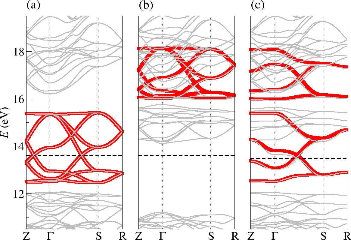
Figure 7: (Color online) DFT band structure (thin lines) for the purely GFO-distorted structure (iii): a) FM majority spin, b) FM minority spin, c) A-AFM. MLWF bands are depicted as thick/red lines. The Fermi level is indicated by dashed lines.

The band dispersion calculated for the purely GFO-distorted structure (iii) is presented in Fig. 7. The rotation and tilting of oxygen octahedra in structure (iii) distorts the ideal 180^∘ Mn-O-Mn bond angle, which is expected to reduce the hopping amplitudes. Indeed, it can be seen in Fig. 7 that the GFO distortion leads to significantly smaller bandwidth (2.951 eV and 2.139 eV for FM majority and minority spin, respectively, compared to 4.126 eV and 3.156 eV in the undistorted structure (i)). As a result, the FM majority spin $e_{g}$ bands become completely separated from the lower-lying $t_{2g}$ bands and the La($d$) bands at higher energy. Unlike in the JT distorted structure (ii), the system stays metallic for both FM and A-AFM order.

Since the unit cell for structure (iii) is quadrupled with respect to the cubic perovskite structure, there are now 8 bands with dominant $e_{g}$ character for each spin direction. However, due to the tilt/rotation of the oxygen octahedra, “$e_{g}$-like” orbitals at a certain site can hybridize with “$t_{2g}$-like” orbitals at a neighboring site, leading to bands with mixed $e_{g}$/$t_{2g}$ character.foo (b) In the FM case this does not represent a problem for the disentanglement procedure, since the bands with predominant $e_{g}$ character are separated from the predominantly $t_{2g}$ bands for both spin direction. For FM order, we can therefore construct four pairs of MLWFs, localized at the four different sites within the unit cell, by defining appropriate energy windows separately for each spin direction. This is not possible in the A-AFM case, where the local minority $t_{2g}$ bands overlap strongly with the local majority $e_{g}$ bands in the energy region between 14 eV and 16 eV. In this case, the standard disentanglement procedure employed for structures (i) and (ii), i.e. defining an energy window $[12.0,21.0]$ eV and initializing 8 Wannier functions from projections on atomic $e_{g}$ orbitals at the various sites, results in MLWFs with mixed $t_{2g}$/$e_{g}$ orbital character. In particular, the resulting local minority spin MLWFs exhibit a rather strong $t_{2g}$ character.

One possible way to overcome this problem would be to construct all 20 $d$-like MLWFs (5 per Mn site), i.e. both $e_{g}$ and $t_{2g}$ orbitals. However, the resulting MLWFs still contain some amount of $e_{g}$/$t_{2g}$ mixing, and the corresponding MLWF matrix elements exhibit systematic deviations from the results obtained in the previous sections, which are derived from a smaller set of MLWFs. In the following, we therefore adopt a different strategy to obtain model parameters for the A-AFM case, and construct the 4 local majority and 4 local minority spin $e_{g}$-like MLWFs separately, using two different energy windows. From this, we obtain the on-site matrix elements $\mathbf{h}^{0}$ as well as the hopping parameters $\mathbf{h}^{x}$ within the $x$-$y$ plane (and of course all further neighbor hopping amplitudes within this plane). On the other hand we do not obtain the hopping amplitudes $\mathbf{h}^{z}$ between adjacent planes in the $z$ direction, which would connect the two separate sets of MLWFs. Similar to the purely JT distorted case, we analyze the effect of the GFO distortion on the $e_{g}$ bands by performing calculations with varying degree of distortion, i.e. by changing the oxygen positions according to Eq. (16). In this case we always adjust the energy window for the construction of the MLWFs to the actual $e_{g}$ bandwidth corresponding to a particular $\alpha_{\mathrm{iii}}$.

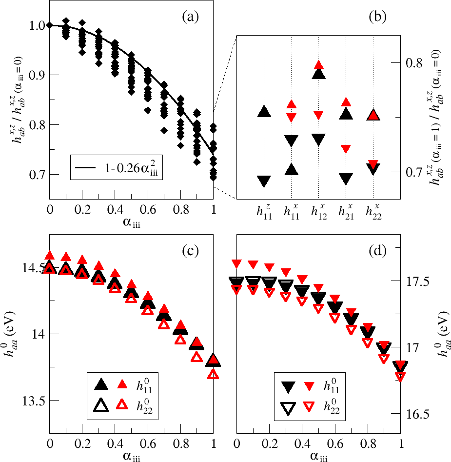
Figure 8: (Color online) Hamiltonian matrix elements in the basis of MLWFs as a function of the GFO distortion. Large/black and small/red symbols correspond to FM and A-AFM order, respectively. Elements associated with purely (local) majority and minority spin character are represented by triangles pointing up and down, respectively.

We find that the main effect of the GFO distortion is indeed a systematic reduction of all hopping amplitudes by $\approx 20-30$ %, consistent with what was reported in Ref. Ederer et al., 2007. Fig. 8a shows the overall reduction for all obtained nearest neighbor hopping amplitudes for both FM and A-AFM order, while Fig. 8b resolves the reduction factors of the various hopping amplitudes for full GFO distortion ($\alpha_{\text{iii}}=1$). It can be seen, that even though there is a significant spread in the reduction factors for the various hopping parameters, the overall reduction can approximately be described as $\mathbf{h}^{x/z}(\alpha_{\mathrm{iii}})=\mathbf{h}^{x/z}(0)\left({1-\eta\alpha^{2}_{\mathrm{iii}}}\right)$, with an average value of $\eta=0.26$.

In addition to the changes in the nearest neighbor hopping amplitudes, we also observe a quadratic decrease of the on-site diagonal matrix elements as a function of the GFO distortion (Fig. 8c/d), with a similar magnitude for both orbitals and different magnetic order. This can be understood again from the underlying hopping between atomic $p$ and $d$ orbitals. Since the effective $e_{g}$ bands correspond to the antibonding combination of these atomic orbitals, a reduction of the underlying $p$-$d$ hopping amplitudes results in a decrease of the $\Gamma$-point energy of the $e_{g}$ states. The Hund’s rule coupling parameter $J=1.502$ eV obtained from the on-site splitting for FM order and $\alpha_{\mathrm{iii}}=1$ is very similar to the corresponding value for the cubic perovskite structure.

III.4 Combined Jahn-Teller and GdFeO₃-type distortion – structure (iv)

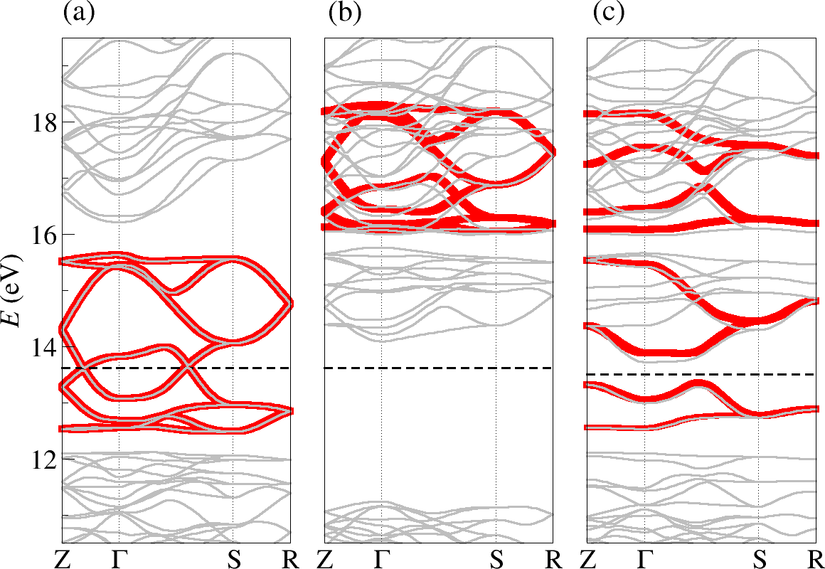
Figure 9: (Color online) DFT band structure (thin lines) for structure (iv): a) majority spin FM, b) minority spin FM, and c) A-AFM. MLWF are depicted as thick/red lines. Fermi level is indicated by dashed line.

So far we have analyzed the individual effects of the JT and GFO distortion. We now discuss whether the superposition of both distortions gives rise to any changes in the MLWF matrix elements that go beyond a simple superposition of the individual effects. The corresponding band structure and MLWF dispersion for structure (iv), i.e. the combined JT and GFO distortion, is presented in Fig. 9. It can be seen that the band structure in this case closely resembles the one of the purely GFO distorted structure (iii), Fig. 7, but with the additional JT-induced effects (avoided band-crossings and lifted degeneracies) as described in Sec. III.2. Note that, as in the purely JT distorted structure, the FM case is metallic, whereas a band gap opens only for A-AFM order.

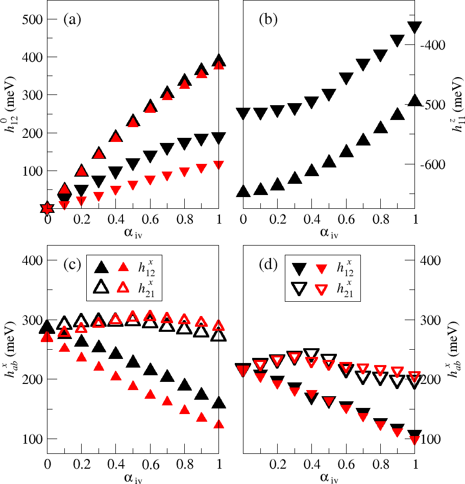
Figure 10: (Color online) MLWF Hamiltonian matrix elements as function of combined JT and GFO distortion. Large/black and small/red symbols correspond to the FM and A-AFM order, respectively. Elements associated with purely (local) majority and minority spin character are represented by triangles pointing up and down, respectively.

As described in the previous section we construct 8 MLWFs per spin direction for the FM case and two separate sets of 4 local majority and 4 local minority $e_{g}$-like MLWFs for the A-AFM case. Fig. 10 shows the evolution of selected MLWF matrix elements as a function of distortion. The atomic positions are changed according to Eq. (16) with $x=\mathrm{iv}$. By comparing Fig. 10a with Fig. 6a, it can be seen that the GFO distortion does also significantly reduce the on-site matrix elements $h_{12}^{0}$ (to $\approx 75-80\,\%$), which are otherwise proportional to the JT distortion. This is further evidence for the ligand-field nature of the JT coupling, i.e. that it is mediated by the Mn-O hybridization (which is reduced by the GFO distortion). Furthermore, it can be seen that the leading hopping along $z$, $h_{11}^{z}$, follows very closely the trend observed for the purely GFO distorted structures. In the case of the off-diagonal hopping amplitudes within the $x$-$y$ plane, the superposition of GFO-distortion-induced reduction and JT-induced splitting leads to an initial increase of $h_{12}^{x}$ for small distortion, followed by a decrease for larger $\alpha_{\mathrm{iv}}$. Overall, the observed trends can indeed be well understood as independent superposition of the individual effects of JT and GFO distortions. We note that the kinks observed in some of the minority spin hopping terms around $\alpha_{\mathrm{iv}}\approx 0.4$ result from the opening of the gap between $e_{g}$-like and $t_{2g}$-like minority spin bands for this amount of distortion, which represents a certain “discontinuity” for the disentanglement procedure.

III.5 Simplified TB models for LaMnO₃ in the full experimental $Pbnm$ structure (v)

The analysis presented so far showed that the effect of different structural distortions on the $e_{g}$ bands can, to a good extent, be treated independently of each other. In this section, we attempt to incorporate the most significant effects described in the previous sections into a refined effective TB model. Then, in order to test the accuracy of the resulting parameterization, we compare the resulting band dispersion with the full GGA and MLWF band-structure, calculated for the full experimental $Pbnm$ structure of LaMnO₃ and A-AFM order.

For the refined TB model we introduce different hopping amplitudes for local majority/minority spin projections to describe the hopping between ferromagnetically aligned nearest neighbors within the $x$-$y$ planes ($t^{\uparrow\uparrow}$/$t^{\downarrow\downarrow}$), and an intermediate value for the nearest neighbor hopping between antiferromagnetically aligned nearest neighbors along the $z$ direction ($t^{\uparrow\downarrow}$), i.e. hopping between two different local spin projections. This is in accordance with our results presented in Sec. III.1. For the corresponding hopping amplitudes we use the values of $h_{11}^{z}$ calculated for the ideal cubic perovskite structure (see Table 2) for FM and A-AFM order, which are then reduced by the same factor $(1-\eta\alpha_{\mathrm{iii}}^{2})$, where $\alpha_{\mathrm{iii}}$ describes the amount of pure GFO distortion. Apart from these modifications we assume the usual cubic symmetry of the nearest neighbor hopping matrices, i.e.:

$$\mathbf{t}^{ss^{\prime}}(\pm a_{\text{c}}\hat{\mathbf{z}}) =(1-\eta\alpha_{\mathrm{iii}}^{2})\,t^{ss^{\prime}}\left(\begin{matrix}1&0\\ 0&0\end{matrix}\right)\ ,$$ (18)

$$\mathbf{t}^{ss^{\prime}}(\pm a_{\text{c}}\hat{\mathbf{x}}) =(1-\eta\alpha_{\mathrm{iii}}^{2})\,t^{ss^{\prime}}\left(\begin{matrix}\tfrac{1}{4}&-\tfrac{\sqrt{3}}{4}\\ -\tfrac{\sqrt{3}}{4}&\tfrac{3}{4}\end{matrix}\right)\ ,$$ (19)

(and analogously for $\mathbf{t}^{ss^{\prime}}(\pm a_{\text{c}}\hat{\mathbf{y}})$). Note that $s$ and $s^{\prime}$ in these equations should be read as a local spin index, i.e. it designates the spin projection relative to the orientation of the local core spin. We use the average value $\eta=0.26$ determined in Sec. III.3.

The JT-induced splitting of the non-diagonal elements of the hopping matrix within the $x$-$y$ plane discussed in Sec. III.2 is incorporated in the TB model as an additional contribution to the in-plane hopping:

$$\Delta\mathbf{t}(\pm a_{\text{c}}\hat{\mathbf{x}})=\tilde{\lambda}Q^{x}_{\mathbf{0}}\alpha_{\mathrm{ii}}(1-\eta\alpha_{\mathrm{iii}})\left(\begin{matrix}0&1\\ -1&0\end{matrix}\right)$$ (20)

(and analogously for $\Delta\mathbf{t}(\pm a_{\text{c}}\hat{\mathbf{y}})$). Here, $\alpha_{\mathrm{ii}}$ describes the amplitude of the staggered JT distortion, i.e. $Q^{x}_{\mathbf{R}}=\pm Q^{x}_{\mathbf{0}}\alpha_{\mathrm{ii}}$, and the parameter $\tilde{\lambda}$ is determined from the average splitting over all hopping amplitudes in the purely JT-distorted structure (shown in Fig. 6c/d). In addition, we include the usual on-site JT effect in essentially the same form as described in Eq. (7), but with a spin-dependent JT coupling constant that is also reduced by the GFO distortion (with the same factor as the hopping amplitudes):

$$\lambda\rightarrow\lambda^{s}(1-\eta\alpha_{\mathrm{iii}}^{2})\ .$$ (21)

We note that the orthorhombic strain in the experimental structure of LaMnO₃ gives rise to a homogeneous $Q^{z}$ component to the JT distortion, i.e. the same $Q^{z}_{\mathbf{R}}\neq 0$ on all sites, which we take into account within the model by using the same coupling constant $\lambda^{s}$ as for the $Q^{x}$ component.

We also include hopping between next nearest neighbors and between second nearest neighbors along the cartesian coordinate axes in the refined TB model, but we do not consider any spin-dependence of the corresponding hopping amplitudes. We describe the hopping between next-nearest neighbors by spin-independent parameters $t^{xy}$ corresponding to the hopping between two $\lvert{3z^{2}-r^{2}}\rangle$-type orbitals along the $\pm a_{\text{c}}\hat{\mathbf{x}}\pm a_{\text{c}}\hat{\mathbf{y}}$ directions. The parameter $t^{xy}$ is taken as spin average over the corresponding MLWF matrix elements $h^{xy}_{11}$ calculated for the cubic structure. All other hopping matrix elements between next nearest neighbors are determined from this via the following relations, which are derived assuming cubic symmetry and indirect hopping only (see Ref. Ederer et al., 2007):

$$\mathbf{t}^{xz} =t^{xy}\left({1-\eta\alpha_{\mathrm{iii}}^{2}}\right)\begin{pmatrix}-2&\sqrt{3}\\ \sqrt{3}&0\end{pmatrix}$$ (22)

$$\mathbf{t}^{xy} =t^{xy}\left({1-\eta\alpha_{\mathrm{iii}}^{2}}\right)\begin{pmatrix}1&0\\ 0&-3\end{pmatrix}$$ (23)

The same GFO-distortion-induced reduction as for the nearest neighbor hopping matrices is applied. The hopping between second nearest neighbors along the coordinate axes [$\mathbf{t}(\pm 2a_{\text{c}}\hat{\mathbf{x}})$, $\mathbf{t}(\pm 2a_{\text{c}}\hat{\mathbf{y}})$, $\mathbf{t}(\pm 2a_{\text{c}}\hat{\mathbf{z}})$] is included according to the ideal cubic symmetry relations described by Eqs. (3)-(5), with $a_{\text{c}}$ replaced by $2a_{\text{c}}$, $t^{\prime}=0$, and $t=t^{2z}$, where $t^{2z}$ is estimated from the MLWF matrix elements for the purely GFO distorted structure. We note that the reduction of this parameter compared to the undistorted case is significantly stronger than for the nearest (and next nearest) neighbor hopping amplitudes. Furthermore, the hopping between third nearest neighbors along the coordinate axes [$\mathbf{t}(\pm 3a_{\text{c}}\hat{\mathbf{x}})$, $\mathbf{t}(\pm 3a_{\text{c}}\hat{\mathbf{y}})$, $\mathbf{t}(\pm 3a_{\text{c}}\hat{\mathbf{z}})$], that was considered in Sec. III.1, becomes negligible as result of the GFO distortion.

Finally, we include the Hund’s rule coupling in the refined TB model using the standard form [Eq. (6)] with an average value of $J$ obtained from the MLWF on-site splitting. In order to relate the obtained TB bands to the full GGA and MLWF band-structures, we determine the on-site energy $e_{0}$ as the spin and orbital average of the corresponding $h_{aa}^{0}$ matrix elements for the A-AFM experimental structure.

The values of all parameters used in the refined TB model are summarized in Table 3. The JT distortion in the experimental $Pbnm$ structure corresponds to $\alpha_{\mathrm{ii}}=1$, $Q^{x}_{\mathbf{0}}=-0.161$ Å, and $Q^{z}=-0.048$ Å, and the corresponding amplitude of the GFO distortion is $\alpha_{\mathrm{iii}}=1$.

Table 3: Parameters used in the TB models.

	refined	simple
$t^{\uparrow\uparrow}$ (eV)	-0.648	-0.492
$t^{\downarrow\downarrow}$ (eV)	-0.512	-0.492
$t^{\uparrow\downarrow}$ (eV)	-0.569	-0.492
$\eta$	0.26	$-$
$\tilde{\lambda}$ (eVÅ-1)	0.53	0
$\lambda^{\uparrow}$ (eVÅ-1)	3.19	1.64
$\lambda^{\downarrow}$ (eVÅ-1)	1.33	1.64
$t^{xy}$ (eV)	-0.018	0
$t^{2z}$ (eV)	-0.020	0
$e_{0}$ (eV)	15.356	15.505
$J$ (eV)	1.5	1.805

We also compare with a very simple TB model that includes only nearest neighbor hopping according to Eqs. (3)-(5) with $t^{\prime}=0$, and the standard JT and Hund’s rule coupling as described by Eqs. (7) and (6). The parameters for this model are chosen via typical simplified fitting procedures: the nearest neighbor hopping parameter $-t$ is obtained as one sixth of the majority spin bandwidth $W$ for the fully GFO distorted structure (iii) and FM order; the JT coupling constant $\lambda$ is taken from Ref. Ederer et al., 2007, where it was obtained by fitting a similar TB model (including also next nearest neighbor hopping) to a DFT band-structure; $J$ is calculated from the spin splitting between FM majority and minority bands at the $\Gamma$-point for the cubic structure (i); and $e_{0}$ is fitted such that the Fermi energy is aligned with the DFT calculation value.

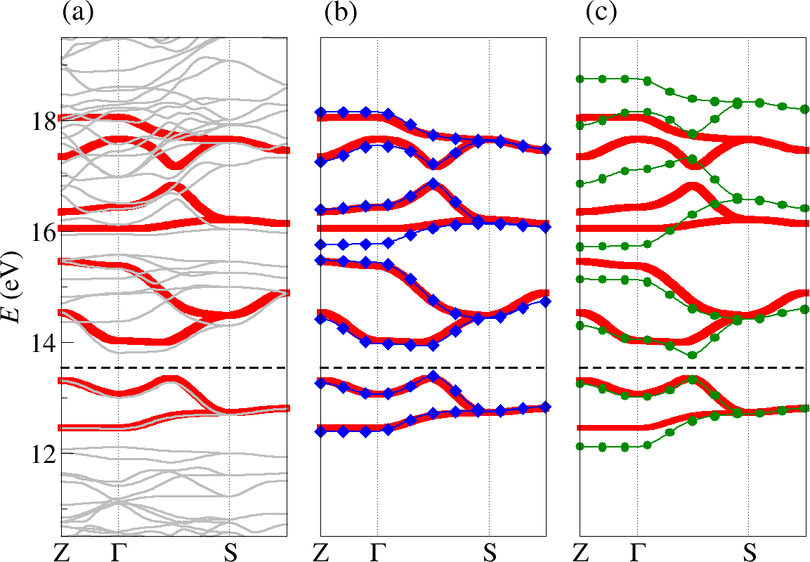
Figure 11: (Color online) (a) DFT bands (thin/grey lines) and MLWF bands (thick/red lines) for the A-AFM experimental $Pbnm$ structure (v). Comparison of the MLWF bands with the refined TB model (b) and with the simple nearest neighbor TB model (c) The Fermi level is indicated by dashed lines.

Figure 11a shows the band dispersion obtained from the GGA calculation for the full experimental structure (v) and A-AFM order as well as the corresponding MLWF bands. Fig. 11b/c shows the comparison between the MLWF bands and the two different simplified TB models. It can be seen that the orthorhombic lattice strain and La displacements do not lead to significant qualitative changes in the band-structure as compared to structure (iv) (see Fig. 9c). The comparison between the MLWF dispersion and the refined TB model (Fig. 11b) shows that, despite the many simplifications made, this model reproduces the MLWF bands to a remarkable accuracy. The only major discrepancy can be seen for the lowest-lying local minority band along $\Gamma$-Z at $E\sim 16$ eV, which is slightly lower than the corresponding MLWF band. This can be traced back to an overestimation of the $h_{22}^{x}$ hopping amplitude, which results from the fact that we use the same reduction factor $\eta$ for all hoppings. As can be seen in Fig. 8b, $h^{x}_{22}$ is affected more strongly by the GFO distortion than any other nearest neighbor hopping (for A-AFM order). The very simple nearest neighbor TB model depicted in Fig. 11c deviates much stronger from the MLWF band structure than the refined model, but still captures the overall dispersion surprisingly well. Consistent with our analysis from the previous sections, the deviations are more pronounced for the energetically higher local minority spin bands, which is clearly due to the neglected spin dependence of the hopping. As discussed in Sec. III.2, the smaller JT coupling constant used in the simple model partially cancels the missing effect of the JT distortion on the inter-orbital in-plane hopping parameters, leading to the relative good agreement of the simpler model with the MLWF bands around the Fermi level.

IV Summary and Conclusions

We have shown that the construction of maximally localized Wannier functions together with the disentanglement procedure described in Ref. Souza et al., 2001 can be used to extract effective $e_{g}$ bands in LaMnO₃ even for cases where these bands are strongly entangled with other states. This procedure thus provides a very robust way for extracting the “correlated subspace” used for example in DFT+DMFT calculations.

We have used this procedure to obtain a TB parameterization of the $e_{g}$ bands for different structural modifications of LaMnO₃ with both FM and A-AFM order. By monitoring the effect of the individual distortions on the MLWF matrix elements, we can assess the quality of the various approximations and simplifications that are commonly used in model Hamiltonians for manganite systems. In particular, we find the following:

• While the nearest neighbor hopping is clearly dominant, the further neighbor hopping along the cartesian axes decays rather slowly. Taking into account nearest, next-nearest, as well as second and third nearest hopping along the cartesian axes leads to deviations of less than 0.11 eV from the (cubic FM) DFT band structure.

• In addition to the linear on-site coupling to the JT distortion, we observe a strong effect on the in-plane hopping amplitudes between different orbitals. The corresponding splitting, which is due to the underlying Mn-O hopping, partially cancels the effect of the on-site term on the band dispersion, which has a strong influence on the determination of the local JT coupling strength.

• The GFO distortion leads to an overall reduction of all hopping amplitudes by about 25-30 %, and also reduces the local JT splitting. This reduction is due to the weaker hybridization between Mn($e_{g}$) and O($p$) states for non-180^∘ bond angle.

• The higher energy of the (local) minority spin states reduces the hybridization between the corresponding atomic $e_{g}$ and O($p$) states, leading to reduced hopping amplitudes and JT coupling compared to the majority spin states.

• The splitting between (local) majority and minority spin states is generally well described by the local Hund’s rule coupling, even though small variations in the corresponding $J$ values indicate the limits of the core spin approximation.

It is apparent that the most crucial deviations from the simple two band description are a result of the underlying Mn-O hybridization. Nevertheless, we have shown that a refined TB model that incorporates the effects described above using the parameters listed in Table 3 reproduces the DFT band structure calculated for the full experimental crystal structure of LaMnO₃ with remarkable accuracy. Whether this accuracy, at the prize of more parameters in the model, is desirable depends of course on the specific application of the model description.

Furthermore, our analysis shows that the effects of the various distinct structural distortions present in LaMnO₃ are (to a good approximation) independent from each other and can therefore be assessed individually. However, the GFO distortion has to be taken into account to obtain the correct magnitude of the Jahn-Teller coupling.

In comparison with the manual TB fits presented in Ref. Ederer et al., 2007, the construction of MLWFs is less biased and more universally applicable. It allows to calculate parameters of the model instead of fitting them to either experimental or computational data. In particular, it is possible to obtain accurate TB representations even for rather complex band structures. However, care has to be applied when parameters corresponding to a more complex parameterization are used for simpler models. For example, using the MLWF nearest neighbor hopping amplitudes within a simple model that neglects all further neighbor hoppings, can lead to a significant underestimation of the total bandwidth, so that in certain cases a parameterization with renormalized nearest neighbor hoppings, leading to a more accurate total bandwidth, might be more desirable. The analysis presented in this work demonstrates that, depending on the specific application at hand, MLWFs can in principle be used to construct more and more refined TB parameterizations which lead to realistic, materials-specific band structures with very high accuracy.