Casimir force waves induced by non-equilibrium fluctuations between vibrating plates

Abstract

We study the fluctuation-induced, time-dependent force between two plates immersed in a fluid driven out of equilibrium mechanically by harmonic vibrations of one of the plates. Considering a simple Langevin dynamics for the fluid, we explicitly calculate the fluctuation-induced force acting on the plate at rest. The time-dependence of this force is characterized by a positive lag time with respect to the driving, indicating a finite speed of propagation of stress through the medium, reminiscent of waves. We obtain two distinctive contributions to the force, where one may be understood as directly emerging from the corresponding force in the static case, while the other is related to resonant dissipation in the cavity between the plates.

I Introduction

A fundamental advance in the understanding of nature was the insight that physical forces between bodies, instead of operating at a distance, are generated by fields; the latter obeying their own dynamics, implying a finite speed of propagation of signals and causality Mullin . Moreover, time-varying fields can sustain themselves in otherwise empty space to produce disembodied waves; exemplified by electromagnetic fields and waves, and gravitational fields. Gravitational waves are believed to be detected in the near future Col04 .

Another force seemingly operating at a distance is the Casimir force. This force was first predicted by Casimir in 1948 for two parallel conducting plates in vacuum, separated by a distance $L$, for which he found an attractive force per unit area $F/A=-\pi^{2}\hbar c/(240L^{4})$ Cas48 . It can be understood as resulting from the modification of the quantum-mechanical zero-point fluctuations of the electromagnetic fields due to confining boundaries M93 ; GK99 ; Mil01 . In the last decade, high-precision measurements of the Casimir force have become available which confirm Casimir’s prediction within a few per cent Lam97 ; MR98 ; Chan1 ; recent experiments demonstrate the possibility of using the Casimir force as an actuation force for movable elements in nanomechanical systems Chan1 ; Chan2 . This development goes along with significant advances in calculating the Casimir force for complex geometries and materials EHGK01 ; E09 ; J09 .

A force analogous to the electrodynamic Casimir force also occurs if the fluctuations of the confined medium are of thermal origin K94 ; GK99 . The thermal analog of the Casimir effect, referred to as critical Casimir effect, was first predicted by Fisher and de Gennes for the concentration fluctuations of a binary liquid mixture close to its critical demixing point confined by boundaries FdG78 ; recently, the critical Casimir effect was quantitatively confirmed for this very system HH08 . (For computational methods concerning the calculation of critical Casimir forces, see, e.g., references HS98 ; V09 .)

The vast majority of work done on the Casimir effect, and fluctuation-induced forces in general, pertain to the equilibrium case. That is, the system is in its quantal ground state in case of the electrodynamic Casimir effect, or in thermodynamic equilibrium in case of the thermal analog. A number of recent experiments probe the Casimir force between moving components in nanomechanical systems Chan1 ; Chan2 , and effects generated by moving boundaries have been studied, e.g., for Casimir force driven ratchets E07 ; however, the data are usually compared with predictions for the Casimir force obtained for systems at rest, corresponding to a quasi-static approximation. Distinct new effects occur if the fluctuating medium is driven out of equilibrium. In this case the observed effects become sensitive to the dynamics governing the fluctuation medium, which may lead to a better understanding of these systems, and may provide new control parameters to manipulate them B03 ; NG04 ; C06 ; B07 ; BS08 . For example, the generalization of the electrodynamic Casimir effect to systems with moving boundaries, referred to as dynamic Casimir effect, exhibits friction of moving mirrors in vacuum and the creation of photons LJR96 ; D96 ; GK98 . For the thermal analog, fluctuation-induced forces in non-equilibrium systems have been studied in the context of the Soret effect, which occurs in the presence of an external temperature gradient NG04 . Fluctuation-induced forces have also been obtained for macroscopic bodies immersed in mechanically driven systems B03 , granular fluids C06 , and reaction-diffusion systems B07 . Recently it was shown that non-equilibrium fluctuations can induce self-forces on single, asymmetric objects, and may lead to a violation of the action-reaction principle between two objects BS08 .

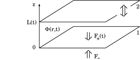
Figure 1: Two parallel plates separated by a varying distance $L(t)$. Plate 1 is at rest while plate 2 is vibrating parallel to the $z$-direction. The plates are immersed in a fluctuating medium described by the order parameter $\phi({\bf r},t)$. The fluctuation-induced, time-dependent net force on plate 1 is the sum of the forces $F_{+}(t)$ and $F_{-}$ acting on opposite sides of the plate.

In this work we consider a fluctuating medium driven out of equilibrium mechanically by a vibrating plate, and study the resulting time-dependent, fluctuation-induced force $F(t)$ on a second plate at rest. We wish to elucidate the time-dependence of this force in view of the finite speed of propagation of signals in the fluctuating medium, and causality. Specifically, we consider two infinitely extended plates parallel to the $xy$-plane separated by a varying distance $L(t)$ as shown in Fig. 1. Plate 1 is at rest while plate 2 is vibrating in $z$-direction by some external driving. The plates are immersed in a medium undergoing thermal fluctuations with long-ranged correlations described by a scalar order parameter $\phi({\bf r},t)$. The order parameter is subject to Dirichlet boundary conditions $\phi=0$ at the plates. As shown in Fig. 1, $F(t)$ is the sum of the forces $F_{+}(t)$ and $F_{-}$ acting on opposite sides of the plate; $F_{+}(t)$ being the force acting on plate 1 from the side of the cavity, and $F_{-}$ the (time-independent) force on the boundary surface of a semi-infinite half-space filled with the fluctuating medium. The net force $F(t)=F_{+}(t)+F_{-}$ is expected to be finite and overall attractive, i.e., directed towards plate 2.

Our presentation is organized as follows. In Sec. II we introduce the Langevin dynamics of the order parameter $\phi({\bf r},t)$ as a paradigmatic example for a non-equilibrium dynamics, and summarize our main results for the fluctuation-induced force $F(t)$. In Sec. III we discuss the calculation of $F(t)$ using the stress tensor (Sec. III.1) and obtain $F(t)$ to first order in the amplitude of the vibrations of plate 2 (Sec. III.2). We find two distinct contributions to $F(t)$, which can be attributed to real-valued poles (Sec. III.3) and imaginary poles (Sec. III.4) in the complex frequency plane, respectively, occurring in the calculation of $F(t)$. We conclude in Sec. IV.

II Model and main results

In the traditional case, both plates are at rest at a constant separation $L_{0}$ (cf. Fig. 1). The system is then in thermal equilibrium and the fluctuations of the order parameter $\phi$ are described by the statistical Boltzmann weight $e^{-\beta{\cal H}}$ with Gaussian Hamiltonian

$$\beta{\cal H}\{\phi\}=\frac{1}{2}\int d^{3}r\,(\nabla\phi)^{2}\,\,,$$ (1)

where $\beta=1/(k_{B}T)$ with the Boltzmann constant $k_{B}$ and the temperature $T$ (assumed to be constant). The fluctuation-induced force $F_{0}$ on plate 1 per unit area $A$ is found to be LK92 ; K94 ; GK99

$$\frac{F_{0}}{A}=-\frac{\xi(3)}{8\pi}\frac{k_{B}T}{L_{0}^{3}}\,\,,$$ (2)

where the minus sign indicates that the force is attractive. Equation (2) is a universal result, independent of the underlying dynamics of the fluctuating medium, as long as the thermodynamic equilibrium is described by Eq. (1).

We now turn to the case where plate 2 is vibrating parallel to the $z$-direction, resulting in a time-dependent separation $L(t)$ to plate 1. The time-dependent boundary conditions for the order parameter $\phi({\bf r},t)$ then drive the system out of equilibrium. Locally, the order parameter will relax back to equilibrium according to the dynamics of the medium; in this work, we consider an overdamped dynamics described by the Langevin equation

$$\gamma\frac{\partial}{\partial t}\phi({\bf r},t)=\nabla^{2}\phi{(\bf r},t)+\eta({\bf r},t)$$ (3)

where $\gamma$ is the friction coefficient. The random force $\eta({\bf r},t)$ is assumed to have zero mean and to obey the fluctuation-dissipation relation

$$\langle\eta({\bf r},t)\eta({\bf r}^{\prime},t^{\prime})\rangle=2\gamma k_{B}T\delta^{(3)}({\bf r}-{\bf r}^{\prime})\delta(t-t^{\prime})$$ (4)

where the brackets $\langle\,\,\,\rangle$ denote a local, stochastic average and $\delta^{(3)}$ is the delta function in 3 dimensions.

Figures 2 - 4 summarize our main results for the case that the external driving $L(t)$ is given by harmonic oscillations

$$L(t)=L_{0}+a\cos(\omega_{0}t)$$ (5)

with amplitude $a$ and frequency $\omega_{0}$. Our results for $F(t)$ hold to first order in $a$ and can be cast in the form

$$F(t)=F_{0}\left[1-\frac{3a}{L_{0}}f(t,\Omega)\right]\,\,+\,{\cal O}(a^{2})$$ (6)

where $F_{0}$ from Eq. (2) is the force for a constant separation $L_{0}$. The dimensionless parameter

$$\Omega=\omega_{0}\gamma L_{0}^{2}$$ (7)

characterizes the strength of the friction coefficient $\gamma$ of the fluctuating medium (cf. Eq. (3)). Equation (6) implies that the dimensionless function $f(t,\Omega)$ is normalized such that $f=1$ for $\omega_{0}=0$, i.e., $\Omega=0$. It can be represented as

$$f(t,\Omega)=A\cos(\omega_{0}t-\varphi)=A\cos[\omega_{0}(t-t_{0})]$$ (8)

in terms of an amplitude $A(\Omega)$ and a phase shift $\varphi(\Omega)$. The second equation in Eq. (8) holds if $\varphi$ is proportional to the driving frequency $\omega_{0}$, i.e., $\varphi(\Omega)=\omega_{0}t_{0}(\Omega)$, where the lag time $t_{0}$ corresponds to the time delay between the source (driving $L(t)$ of plate 2) and the resulting response (force $F(t)$ at plate 1). For the relation $\varphi(\Omega)=\omega_{0}t_{0}(\Omega)$ used to obtain the second equation in Eq. (8) it is understood that $t_{0}(\Omega)$ depends on $\Omega$ only weakly so that, in particular, $t_{0}(0)$ is finite.

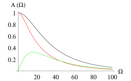
Figure 2: Amplitude $A$ of $f(t,\Omega)$ as a function of $\Omega$ (see Eq. (8)). Shown are results for $F(t)$ (black line) and for the contributions to $F(t)$ according to Eq. (33) (red line) and Eq. (35) (green line), respectively.

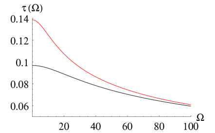
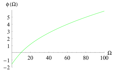
Figure 3: (a) Lag time $t_{0}$ in terms of the dimensionless combination $\tau=t_{0}/(\gamma L_{0}^{2})$ as a function of $\Omega$ (see Eq. (8)). Shown are results for $F(t)$ (black line) and for the contribution to $F(t)$ according to Eq. (33) (red line). In both cases, the dependence $\tau(\Omega)$, i.e., $t_{0}(\omega_{0})$, is fairly weak, so that the interpretation of $t_{0}$ as a lag time is justified. (b) Phase shift $\varphi$ as a function of $\Omega$ (see Eq. (8)) for the contribution to $F(t)$ according to Eq. (35). In this case, $t_{0}=\varphi/\omega_{0}$ strongly depends on $\omega_{0}$.

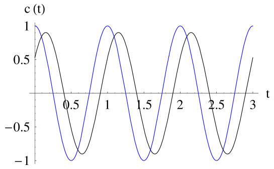
Figure 4: $c(t)=F(t)/F_{0}$ according to Eq. (6) for $\omega_{0}=2\pi\,\text{s}^{-1}$ and $\Omega=10$ (black line). The function $\cos(\omega_{0}t)$, corresponding to the oscillating part of $L(t)$ with $a=1$ (cf. Eq. (5)) is also shown (blue line). The lag time for these parameters is $t_{0}=\tau(\Omega)\Omega/\omega_{0}\simeq 0.15\,\text{s}$.

Figure 2 shows the amplitude $A(\Omega)$ of the function $f(t,\Omega)$ according to Eq. (8) (black line). The contribution to $F(t)$ according to Eqs. (33) and (35), corresponding to real-valued poles and imaginary poles in the complex frequency plane occurring in the calculation of $F(t)$, are also shown (red and green lines, respectively); cf. Secs. III.3 and III.4 below. Figure 3a shows the lag time $t_{0}(\Omega)$ according to Eq. (8) in terms of the dimensionless combination $\tau=t_{0}/(\gamma L_{0}^{2})$. Shown are results for $F(t)$ (black line) and for the contribution to $F(t)$ according to Eq. (33) (red line). In both cases, the dependence $\tau(\Omega)$, i.e., $t_{0}(\omega_{0})$, is fairly weak, so that the interpretation of $t_{0}$ as a lag time is justified. Thus, the form of $f(t,\Omega)$ in Eq. (8), in conjunction with an approximately constant lag time $t_{0}$, indicates that the stress generated locally at the vibrating plate 2 is carried through the medium, according to its diffusive dynamics, until it arrives at plate 1 after a time $t_{0}\sim\gamma L_{0}^{2}$. This indicates that the fluctuation-induced force on plate 1 is indeed not operating at a distance, but generated by a local field, which for the present system is presumably related to the local stress in the fluctuating medium between the plates. In contrast, Fig. 3b shows that for the contribution to $F(t)$ according to Eq. (35), the phase shift $\varphi$ rather than $t_{0}$ is fairly constant, which implies that $t_{0}=\varphi/\omega_{0}$ strongly depends on $\omega_{0}$. Note, however, that for small $\omega_{0}$, i.e., small $\Omega$, the corresponding contribution to $F(t)$ is suppressed by a vanishing amplitude $A(\Omega)$ (green line in Fig. 2). For illustration, Fig. 4 shows the time-dependent force $F(t)$, normalized by its value $F_{0}$ for $\omega_{0}=0$, for the values $\omega_{0}=2\pi\,\text{s}^{-1}$ and $\Omega=10$ (black line). The function $\cos(\omega_{0}t)$, corresponding to the oscillating part of $L(t)$ with $a=1$ (cf. Eq. (5)), is also shown (blue line). The lag time for these parameters is $t_{0}=\tau(\Omega)\Omega/\omega_{0}\simeq 0.15\,\text{s}$.

III Method

III.1 Calculation of $F(t)$ using the stress tensor

The force per unit area acting on plate 1 from the side of the cavity can be expressed as $F_{+}(t)/A=\lim\limits_{z\to 0}\langle T_{zz}({\bf r}_{\parallel},z,t)\rangle$ where ${\bf r}_{\parallel}=(x,y)$ are the components of ${\bf r}$ parallel to the plate and $T_{zz}=\frac{1}{2}\left(\partial_{z}\phi\right)^{2}-\frac{1}{2}\left[\left(\partial_{x}\phi\right)^{2}+\left(\partial_{y}\phi\right)^{2}\right]$ is the $zz$-component of the stress tensor, assuming the system is locally in equilibrium Mil01 ; GD06 . Similarly, the force per unit area acting on the other side of plate 1 obtains as $F_{-}/A=-\lim\limits_{z\to 0}\langle T_{zz}({\bf r}_{\parallel},z,t)\rangle_{L=\infty}$ where $T_{zz}$ is again evaluated in the cavity between the plates but for the limit $L\to\infty$ (cf. Fig. 1). The net force per unit area on plate 1 obtains as

$$\frac{F(t)}{A}=\lim_{z\to 0}\langle T_{zz}({\bf r}_{\parallel},z,t)\rangle-\lim_{z\to 0}\langle T_{zz}({\bf r}_{\parallel},z,t)\rangle_{L=\infty}$$ (9)

where, using the Dirichlet boundary condition $\phi=0$ at the plates,

$$\lim_{z\to 0}\langle T_{zz}({\bf r}_{\parallel},z,t)\rangle=\frac{1}{2}\lim_{z,z^{\prime}\to 0}\partial_{z}\partial_{z^{\prime}}\langle\phi({\bf r}_{\parallel},z,t)\phi({\bf r}_{\parallel},z^{\prime},t)\rangle\,\,.$$ (10)

To calculate the two-point correlation function of $\phi$ on the right-hand side of Eq. (10) we note that the solution $\phi({\bf r},t)$ of Eq. (3) can be expressed as

$$\phi({\bf r},t)=\int\limits_{-\infty}^{\infty}dt^{\prime}\int\limits_{V(t^{\prime})}d^{3}r^{\prime}G({\bf r},t;{\bf r}^{\prime},t^{\prime})\eta({\bf r}^{\prime},t^{\prime})$$ (11)

where $V(t^{\prime})=A\cdot L(t^{\prime})$ is the volume of the cavity at time $t^{\prime}$ and the Green’s function $G({\bf r},t;{\bf r}^{\prime},t^{\prime})$ is defined as the solution of

$$\left(\gamma\frac{\partial}{\partial t}-\nabla_{r}^{2}\right)G({\bf r},t;{\bf r}^{\prime},t^{\prime})=\delta^{(3)}({\bf r}-{\bf r}^{\prime})\delta(t-t^{\prime})$$ (12)

subject to the boundary condition $G({\bf r},t;{\bf r}^{\prime},t^{\prime})=0$ whenever ${\bf r}$ or ${\bf r}^{\prime}$ is located on the surface of one of the plates at time $t$ or $t^{\prime}$, respectively. In addition, $G({\bf r},t;{\bf r}^{\prime},t^{\prime})=0$ for $t^{\prime}>t$ by causality. Thus, $\phi({\bf r},t)$ can be expressed as a linear superposition of contributions from the source $\eta({\bf r}^{\prime},t^{\prime})$ at times $t^{\prime}<t$ and positions ${\bf r}^{\prime}\in V(t^{\prime})$, carried forward in time by the propagator $G({\bf r},t;{\bf r}^{\prime},t^{\prime})$. Using Eqs. (11) and (4), the two-point correlation function of $\phi$ obtains as

$$\langle\phi({\bf r},t)\phi({\bf r}^{\prime},t^{\prime})\rangle=2\gamma k_{B}T\int\limits_{-\infty}^{\infty}ds\int\limits_{V(s)}d^{3}x\,G({\bf r},t;{\bf x},s)G({\bf r}^{\prime},t^{\prime};{\bf x},s)\,\,.$$ (13)

In the present set-up, the system is translationally invariant in $xy$-direction at any time $t$, whereas translation invariance in time is broken due to the varying separation $L(t)$ between the plates. Thus, introducing the partial Fourier transform $g$ of $G$ as

$$G({\bf r}_{\parallel},z,t;{\bf r}_{\parallel}^{\prime},z^{\prime},t^{\prime})=\int\frac{d^{2}p}{(2\pi)^{2}}\,e^{i{\bf p}\cdot({\bf r}_{\parallel}-{\bf r}_{\parallel}^{\prime})}\int\limits_{-\infty}^{\infty}\frac{d\omega}{2\pi}\,e^{-i\omega(t-t^{\prime})}\,g(z,z^{\prime};\omega,p,t^{\prime})\,\,,$$ (14)

the function $g$ depends explicitly on one of the time coordinates in $G$, say, $t^{\prime}$. Using Eqs. (13), (14) we find for the expression in Eq. (10) remcc

$$\lim_{z\to 0}\langle T_{zz}({\bf r}_{\parallel},z,t)\rangle=\gamma k_{B}T\int\frac{d^{2}p}{(2\pi)^{2}}\int\limits_{-\infty}^{\infty}\frac{d\omega}{2\pi}\int\limits_{0}^{L(t)}d\zeta\,u(\zeta,\omega,p,t)\,u^{*}(\zeta,\omega,p,t)$$ (15)

where

$$u(\zeta,\omega,p,t)=\frac{\partial}{\partial z}g(z,\zeta;\omega,p,t)\Big{|}_{z=0}\,\,.$$ (16)

For given propagator $G$, hence function $u$, $F(t)/A$ can be calculated using Eqs. (9) and (15).

III.2 Calculation of the propagator $G$

The remaining task is to calculate the propagator $G({\bf r},t;{\bf r}^{\prime},t^{\prime})$ solving Eq. (12) subject to the time-dependent boundary conditions due to the vibrating plate 2. This problem can be solved, for general modulations of the plate(s) in space and time, by the method developed in reference HK01 . For the present set-up, we find for the partial Fourier transform ${\cal G}(z,t;z^{\prime},t^{\prime};p)$ of $G$ (i.e., transforming the spatial coordinates ${\bf r}_{\parallel}$, ${\bf r}_{\parallel}^{\prime}$ parallel to the plates as in Eq. (14) but keeping the time coordinates $t$, $t^{\prime}$; in what follows, we omit the argument $p$ for ease of notation) HK01

$${\cal G}(z,t;z^{\prime},t^{\prime}) = \bar{\cal G}(z,t;z^{\prime},t^{\prime})-\int\limits_{-\infty}^{\infty}d\tau\int\limits_{-\infty}^{\infty}d\sigma$$

$$\bar{\cal G}[z,t;L(\tau),\tau]\,{\cal M}(\tau,\sigma)\,\bar{\cal G}[L(\sigma),\sigma;z^{\prime},t^{\prime}]$$

where $\bar{\cal G}$ is the propagator in the half-space $z>0$ bounded by a Dirichlet surface at $z=0$ rem1 . The kernel ${\cal M}$ is defined by

$$\int\limits_{-\infty}^{\infty}d\sigma\,{\cal M}(\tau,\sigma)\,\bar{\cal G}[L(\sigma),\sigma;L(t),t]=\delta(\tau-t)\,\,.$$ (18)

In this work, we consider small variations of the separation between the plates about a mean separation $L_{0}$, i.e.,

$$L(t)=L_{0}+h(t)\,\,.$$ (19)

Our results hold to first order in $h$. To this end, we insert Eq. (19) in Eq. (III.2) and expand everything to first order in $h$ rem2 . This results in expansions $g=g_{0}+g_{1}+{\cal O}(h^{2})$ and $u=u_{0}+u_{1}+{\cal O}(h^{2})$ of the functions $g$ and $u$ from Eqs. (14), (16) in powers of $h$. Equations (9), (15) then yield the corresponding contributions to $F(t)/A$.

Let us first consider the leading order, i.e., $h=0$ and $L(t)=L_{0}$. Using Eq. (III.2) and transforming to $\omega$-space as in Eq. (14) we find (omitting the arguments $p$ and $\omega$ for ease of notation)

$$g_{0}(z,z^{\prime})=\bar{g}(z,z^{\prime})-\bar{g}(z,L_{0})\,M_{0}\,\bar{g}(L_{0},z^{\prime})$$ (20)

where $\bar{g}(z,z^{\prime})=\left[e^{-Q|z-z^{\prime}|}-e^{-Q(z+z^{\prime})}\right]/(2Q)$ with $Q=\sqrt{p^{2}-i\gamma\omega}$ from Eq. (24) below and $M_{0}=[\bar{g}(L_{0},L_{0})]^{-1}=2Q/[1-\exp(-2QL_{0})]$. Thus,

$$g_{0}(z,z^{\prime})=\frac{\sinh(Qz)\sinh[Q(L_{0}-z^{\prime})]}{Q\sinh(QL_{0})}\quad,\,\,z<z^{\prime}\,,$$ (21)

and, using Eq. (16),

$$u_{0}(\zeta)=\frac{\partial}{\partial z}g_{0}(z,\zeta)\Big{|}_{z=0}=\frac{\sinh[Q(L_{0}-\zeta)]}{\sinh(QL_{0})}\,\,.$$ (22)

Using Eqs. (9), (15), (22) we thus obtain to leading order NG04

$$\frac{F_{0}}{A} = -\frac{k_{B}T}{2}\int\frac{d^{2}p}{(2\pi)^{2}}\int\limits_{-\infty}^{\infty}\frac{d\omega}{2\pi i}\,\frac{1}{\omega+i\varepsilon}\left(Q\left[\coth(QL_{0})-1\right]-P\left[\coth(PL_{0})-1\right]\right)$$ (23a)

$$= -\frac{k_{B}T}{2}\int\frac{d^{2}p}{(2\pi)^{2}}\,p\left[\coth(pL_{0})-1\right]\,\,.$$ (23b)

The integral in Eq. (23b) is finite and yields Eq. (2). In Eq. (23a) we use

$$Q(\omega,p)=\sqrt{p^{2}-i\gamma\omega}\,\,\,,\,\,P(\omega,p)=\sqrt{p^{2}+i\gamma\omega}\,\,,$$ (24)

so that $P=Q^{*}$ if $\omega$ is real. Integrations over $\omega$ as in Eq. (23a) are readily computed by contour integration in the complex $\omega$-plane. In Eq. (23a) and throughout this work we use the convention that in $\omega$-integrations we integrate above the pole in $\omega$; this can be accomplished by the replacement $\omega\to\omega+i\varepsilon$ in the denominator of the integrand in Eq. (23a). The limit $\varepsilon\to 0$ in final results is always understood. Note that this prescription introduces a positive time direction and ensures causality. $Q(\omega)$ has a branch cut along the negative imaginary axis $\gamma\omega=-i(p^{2}+r)$, $r\geq 0$, whereas $P(\omega)$ has a branch cut along the positive imaginary axis $\gamma\omega=i(p^{2}+r)$, $r\geq 0$. The integral over $\omega$ in Eq. (23a) has two contributions. For the contribution involving $Q\left[\coth(QL_{0})-1\right]$, the contour integral can be closed in the upper complex $\omega$-plane (thus avoiding the branch cut of $Q$), where this term has no poles, so that the contribution from this term vanishes. Likewise, for the contribution involving $P\left[\coth(PL_{0})-1\right]$, the contour integral can be closed in the lower complex $\omega$-plane (avoiding the branch cut of $P$), where, in turn, this term has no poles. The single pole at $\omega=-i\varepsilon$ in the lower complex $\omega$-plane then yields the expression in Eq. (23b); cp. Fig. 5a in Sec. III.3 with $\omega_{0}=0$.

We now turn to the contribution to $F(t)/A$ to first order in $h$. Using the expansion

$$u(\zeta;\omega,p,t)=u_{0}(\zeta;\omega,p)+u_{1}(\zeta;\omega,p,t)+{\cal O}\left(h^{2}\right)$$ (25)

in Eq. (15), with $u$ from Eq. (16) and $u_{0}$ from Eq. (22), we find for general $h(t)$

$$\frac{F_{1}(t)}{A}=\frac{k_{B}T}{2}\int\frac{d^{2}p}{(2\pi)^{2}}\int\limits_{-\infty}^{\infty}\frac{d\omega}{2\pi}\left[f(\omega,p,t)+f^{*}(\omega,p,t)\right]$$ (26)

where

$$f(\omega,p,t)=\frac{Q}{\sinh(QL_{0})}\stackrel{{\scriptstyle h}}{{\circ}}\frac{1}{i\omega}\left[\frac{Q}{\sinh(QL_{0})}-\frac{P}{\sinh(PL_{0})}\right]\,\,.$$ (27)

The symbol $\stackrel{{\scriptstyle h}}{{\circ}}$ denotes a convolution of two functions $\hat{a}(\omega)$, $\hat{b}(\omega)$ involving an insertion of $h(t)=\int_{-\infty}^{\infty}\frac{d\omega}{2\pi}\exp(-i\omega t)\hat{h}(\omega)$:

$$(\hat{a}\stackrel{{\scriptstyle h}}{{\circ}}\hat{b})(\omega,t^{\prime})=\hat{a}(\omega)\int\limits_{-\infty}^{\infty}\frac{d\omega^{\prime}}{2\pi}e^{-i(\omega-\omega^{\prime})t^{\prime}}\hat{h}(\omega-\omega^{\prime})\hat{b}(\omega^{\prime})\,\,.$$ (28)

For functions $a(t,t^{\prime})$, $b(t,t^{\prime})$, the expression $(\hat{a}\stackrel{{\scriptstyle h}}{{\circ}}\hat{b})(\omega,t^{\prime})$ is the representation in $\omega$-space of $c(t,t^{\prime}):=\int_{-\infty}^{\infty}ds\,a(t,s)h(s)b(s,t^{\prime})$; i.e., $c(t,t^{\prime})=\int_{-\infty}^{\infty}\frac{d\omega}{2\pi}\exp[-i\omega(t-t^{\prime})](\hat{a}\stackrel{{\scriptstyle h}}{{\circ}}\hat{b})(\omega,t^{\prime})$. The functions $\hat{a}(\omega)$, $\hat{b}(\omega)$ are the representations in $\omega$-space of $a(t,s)$, $b(s,t^{\prime})$, respectively rem .

For the special case that plate 2 is vibrating with harmonic oscillations of amplitude $a$ and frequency $\omega_{0}$ (cf. Eqs. (5), (19)), i.e.,

$$h(t)=a\cos(\omega_{0}t)\,\,,$$ (29)

we obtain $\hat{h}(\omega)=a\pi\left[\delta(\omega-\omega_{0})+\delta(\omega+\omega_{0})\right]$. The integral $\int_{-\infty}^{\infty}\frac{d\omega}{2\pi}(f+f^{*})$ in Eq. (26) decays into two contributions corresponding to the terms in square brackets on the right-hand side of Eq. (27):

$$\int\limits_{-\infty}^{\infty}\frac{d\omega}{2\pi}\left[f(\omega,p,t)+f^{*}(\omega,p,t)\right]=\Phi_{QQ}(p,t)+\Phi_{QP}(p,t)\,\,,$$ (30)

where the subscripts QQ and QP indicate the contributions from the first and second term in square brackets of Eq. (27), respectively. In what follows we show that these two terms yield distinct contributions to $F(t)$ corresponding to real-valued and imaginary poles in the complex $\omega$-plane.

III.3 Real-valued frequency poles: lag time $t_{0}$

For the first contribution in Eq. (30) we find remcc ; eps

$$\Phi_{QQ}(p,t)=\frac{a}{2}\,e^{-i\omega_{0}t}\int\limits_{-\infty}^{\infty}\frac{d\omega}{2\pi i}\left[\frac{u(\omega)u(\omega-\omega_{0})}{\omega-\omega_{0}+i\varepsilon}-\frac{v(\omega)v(\omega+\omega_{0})}{\omega+\omega_{0}+i\varepsilon}\right]\,\,+\,c.c.$$ (31)

where

$$u(\omega)=\frac{Q}{\sinh(QL_{0})}\,\,,\,\,\,v(\omega)=\frac{P}{\sinh(PL_{0})}\,\,,$$ (32)

with $Q$, $P$ from Eq. (24). Computing the right-hand side of Eq. (31) by contour integration in the complex $\omega$-plane, the contributions from the two terms in square brackets in the integrand are analyzed along similar lines as discussed below Eq. (24). Thus, for the first term in square brackets, the contour integral can be closed in the upper complex $\omega$-plane, where $u(\omega)$ has no poles, so that the contribution from this term vanishes. For the second term in square brackets, the contour integral can be closed in the lower complex $\omega$-plane, where $v(\omega)$ has no poles. The only contribution from this term is from the single pole at $\omega=-\omega_{0}-i\varepsilon$; see Fig. 5a. Thus, including the contribution from the complex conjugate in Eq. (31), we obtain

$$\Phi_{QQ}(p,t)=\frac{ap}{2\sinh(pL_{0})}\left[e^{i\omega_{0}t}v(\omega_{0})+e^{-i\omega_{0}t}u(\omega_{0})\right]\,\,.$$ (33)

The corresponding contribution to $F_{1}(t)/A$ is given by $\frac{k_{B}T}{2}\int\frac{d^{2}p}{(2\pi)^{2}}\Phi_{QQ}(p,t)$ (see Eqs. (26) and (30)). In the static case, where $\omega_{0}=0$ and $h(t)=a$ in Eq. (5), this result can also be obtained directly from Eq. (23b) by replacing $L_{0}$ with $L_{0}+a$ and expanding to first order in $a$. For finite $\omega_{0}$, Eq. (33) emerges from the static case by a shift from $\omega_{0}=0$ to a finite value of $\omega_{0}$. This shift may be understood in terms of a transition from stationary modes (standing waves) in the cavity in the static case to modes with a time-dependence $\sim\exp(i\omega_{0}t)$, reminiscent of traveling waves, in response to the oscillating plate 2. The time-dependence of these modes carries over to the fluctuation-induced force on plate 1 (cf. Fig. 1). The picture of traveling waves in the fluctuating medium with a finite speed of propagation (diffusion) is consistent with the presence of a lag time $t_{0}\sim\gamma L_{0}^{2}$ in Eq. (8), where $t_{0}>0$ by causality; cf. Fig. 3a and the related discussion in Sec. II.

III.4 Imaginary frequency poles: Resonant dissipation

For the second contribution in Eq. (30) we find eps

$$\Phi_{QP}(p,t)=-\frac{a}{2}\,e^{-i\omega_{0}t}\omega_{0}\int\limits_{-\infty}^{\infty}\frac{d\omega}{2\pi i}\left[\frac{u(\omega)v(\omega-\omega_{0})}{(\omega-\omega_{0}+i\varepsilon)(\omega+i\varepsilon)}\right]\,\,+\,c.c.$$ (34)

The contour integral over $\omega$ can be closed either in the upper or the lower complex $\omega$-plane, yielding identical results; the contributions from the poles at $\omega=\omega_{0}-i\varepsilon$ and $\omega=-i\varepsilon$ in the lower complex $\omega$-plane cancel. Closing the contour integral in the lower plane, the integral picks up contributions from the imaginary poles $\gamma\omega_{n}=-i(p^{2}+k_{n}^{2})$ of $u(\omega)$, where $k_{n}=n\pi/L_{0}$ and $n\geq 1$ is a positive integer. Note that $u(\omega)$ has a branch cut along the negative imaginary axis on which the poles $\omega_{n}$ are located (cf. the related discussion below Eq. (24)); however, this branch cut may be cured using the identity $Q/\sinh(QL_{0})=R/\sin(RL_{0})$, with $R(\omega,p)=\sqrt{i\gamma\omega-p^{2}}$, which holds close to the negative imaginary axis. The expression $R/\sin(RL_{0})$ is analytic in the lower complex $\omega$-plane with isolated poles at $\omega_{n}$; see Fig. 5b. Summing over the residues of these poles yields

$$\Phi_{QP}(p,t)=a\,e^{-i\omega_{0}t}\,\frac{i\gamma\omega_{0}}{L_{0}}\sum_{n=1}^{\infty}(-1)^{n}\frac{v(\omega_{n}-\omega_{0})\,k_{n}^{2}}{(p^{2}+k_{n}^{2})(p^{2}+k_{n}^{2}-i\gamma\omega_{0})}\,\,+\,c.c.$$ (35)

The corresponding contribution to $F_{1}(t)/A$ is given by $\frac{k_{B}T}{2}\int\frac{d^{2}p}{(2\pi)^{2}}\Phi_{QP}(p,t)$. Note that $\Phi_{QP}(p,t)$ is proportional to $\omega_{0}$, which implies that this term is absent in the static case $\omega_{0}=0$ and solely generated by the fact that the system is driven out of equilibrium by the oscillating plate. The imaginary poles $\gamma\omega_{n}=-i(p^{2}+k_{n}^{2})$ leading to Eq. (35) are related to the dissipation in the medium. The poles $\omega_{n}$ thus correspond to resonant dissipation, where the spectrum of resonance frequencies $p^{2}/\gamma+n^{2}\pi^{2}/(\gamma L^{2})$ is continuous due to the presence of the continuous in-plane wave number $p$ dis .

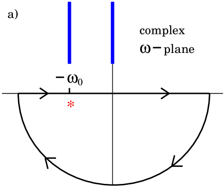
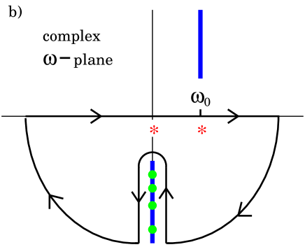
Figure 5: (a) Contour integration in the complex $\omega$-plane for the second term in square brackets in Eq. (31). The only contribution from this term is from the pole at $\omega=-\omega_{0}-i\varepsilon$ indicated by the red star. The blue lines indicate branch cuts of $v(\omega)v(\omega+\omega_{0})$. (b) Contour integration in the complex $\omega$-plane in Eq. (34). The blue lines indicate branch cuts of of $u(\omega)v(\omega-\omega_{0})$. The contributions from the poles at $\omega=\omega_{0}-i\varepsilon$ and $\omega=-i\varepsilon$ cancel (see text).

IV Concluding Remarks

We have studied the time-dependent, fluctuation-induced force $F(t)$ on a plate at rest generated by a second plate with harmonic oscillations (cf. Fig.1). Our main results, valid to first order in the amplitude $a$ of the oscillations (cf. Eq. (5)) and summarized in Figs. 2 - 4, indicate that the fluctuation-induced force is carried through the medium from one plate to the other with a finite speed of propagation (diffusion). We find two distinct contributions to $F(t)$, related to real-valued poles and imaginary poles in the complex frequency plane, resulting in a finite lag time $t_{0}$ in Eq. (8) and resonant dissipation (Secs. III.3 and III.4). In this work we consider a scalar order parameter $\phi({\bf r},t)$ with overdamped dynamics described by the Langevin equation (cf. Eq. (3)). However, our approach can be readily applied to other dynamical systems. In particular, it would be interesting to extend this study to the time dependence of the electrodynamic Casimir force.

References

References

- (1) E. McMullin, The Origins of the Field Concept in Physics, Phys. Perspect. 4, 13 (2002).
- (2) H. Collins, Gravity’s Shadow: The Search For Gravitational Waves (University of Chicago Press, Chicago, 2004).
- (3) H. B. G. Casimir, Proc. K. Ned. Akad. Wet. 51, 793 (1948).
- (4) P. W. Milonni, The Quantum Vacuum: An Introduction to Quantum Electrodynamics (Academic, San Diego, 1993).
- (5) R. Golestanian and M. Kardar, Rev. Mod. Phys. 71, 1233 (1999).
- (6) K. A. Milton, The Casimir Effect (World Scientific, Singapore, 2001).
- (7) S. K. Lamoreaux, Phys. Rev. Lett. 78, 5 (1997).
- (8) U. Mohideen and A. Roy, Phys. Rev. Lett. 81, 4549 (1998).
- (9) H. B. Chan, V. A. Aksyuk, R. N. Kleiman, D. J. Bishop, and F. Capasso, Science 291, 1941 (2001); Phys. Rev. Lett. 87, 211801 (2001).
- (10) F. Capasso, J. N. Munday, D. Iannuzzi, and H. B. Chan, IEEE J. Sel. Top. Quantum Electron. 13, 400 (2007).
- (11) T. Emig, A. Hanke, R. Golestanian, and M. Kardar, Phys. Rev. Lett. 87, 260402 (2001); Phys. Rev. A 67, 022114 (2003).
- (12) T. Emig, Casimir Forces and Geometry in Nanosystems, in G. Radons, B. Rumpf, and H. G. Schuster, Editors, Nonlinear Dynamics of Nanosystems (Wiley, New York, 2009).
- (13) M. T. H. Reid, A. W. Rodriguez, J. White, and S. G. Johnson, Phys. Rev. Lett. 103, 040401 (2009); A. W. Rodriguez, A. P. McCauley, J. D. Joannopoulos, and S. G. Johnson, Phys. Rev. A 80, 012115 (2009).
- (14) M. Krech, The Casimir Effect in Critical Systems (World Scientific, Singapore, 1994).
- (15) M. E. Fisher and P.-G. de Gennes, C. R. Acad. Sci. Paris B 287, 207 (1978).
- (16) C. Hertlein, L. Helden, A. Gambassi, S. Dietrich, and C. Bechinger, Nature 451, 172 (2008).
- (17) A. Hanke, F. Schlesener, E. Eisenriegler, and S. Dietrich, Phys. Rev. Lett. 81, 1885 (1998); F. Schlesener, A. Hanke, and S. Dietrich, J. Stat. Phys. 110, 981 (2003).
- (18) O. Vasilyev, A. Gambassi, A. Maciolek, and S. Dietrich, Phys. Rev. E 79, 041142 (2009).
- (19) T. Emig, Phys. Rev. Lett. 98, 160801 (2007).
- (20) D. Bartolo, A. Ajdari, and J.-B. Fournier, Phys. Rev. E 67, 061112 (2003).
- (21) A. Najafi and R. Golestanian, Europhys. Lett. 68, 776 (2004).
- (22) C. Cattuto, R. Brito, U. M. B. Marconi, F. Nori, and R. Soto, Phys. Rev. Lett. 96, 178001 (2006).
- (23) R. Brito, U. M. B. Marconi, and R. Soto, Phys. Rev. E 76, 011113 (2007).
- (24) P. R. Buenzli and R. Soto, Phys. Rev. E 78, 020102 (2008).
- (25) A. Lambrecht, M.-T. Jaekel, and S. Reynaud, Phys. Rev. Lett. 77, 615 (1996).
- (26) P. Davis, Nature (London) 382, 761 (1996).
- (27) R. Golestanian and M. Kardar, Phys. Rev. A 58, 1713 (1998).
- (28) For an account of the critical dynamics in thin films corresponding to model A, see A. Gambassi and S. Dietrich, J. Stat. Phys. 123, 929 (2006).
- (29) H. Li and M. Kardar, Phys. Rev. A 46, 6490, (1992).
- (30) The star and symbols indicate the complex conjugate for real-valued argument .
- (31) A. Hanke and M. Kardar, Phys. Rev. Lett. 86, 4596 (2001); Phys. Rev. E 65, 046121 (2002).
- (32) That is, the function itself is independent of the vibrating plate 2; the dependence of on plate 2 in Eq. (III.2) only enters through the arguments , in , and the kernel .
- (33) Note that also enters the upper boundary of the integration over in Eq. (15).
- (34) Equations (26), (27) are obtained by using Eq. (III.2) with , expanding everything to first order in , and using Eq. (28) for the resulting insertions of . The contribution of to first order in is determined by Eq. (18), resulting in where the subscripts 0 and 1 indicate the order in . is given below Eq. (20).
- (35) Regarding the replacement in the denominator of the integrand, see the discussion below Eq. (24).
- (36) Compare the related discussion of resonant dissipation in the context of the dynamic Casimir effect in reference GK98 .