Elementary Excitations in Bose-Einstein Condensates at Large Scattering Lengths

Abstract

We present a theoretical analysis of excitation modes in Bose-Einstein condensates in ultracold alkali-metal gases for large scattering lengths and momenta where corrections to the mean field approximation become important. We assume that the effective interaction in the metastable, single channel, gaseous phase has a well defined Fourier transform that scales with the scattering length. Based on this we show that for increasing scattering lengths or equivalently increasing densities the system becomes less correlated and that at large values of the scattering length Bragg scattering measures directly the Fourier transform of the effective two-body potential. We construct model potentials which fit the recently measured line shifts in ⁸⁵Rb by Papp et al. (Phys. Rev. Lett. 101, 135301 (2008)), and show that they fix the low momentum expansion of the effective range function. We find excellent agreement with the experimental data when the effective range is $\ll 1$ and the coefficient of the $k^{4}$-term is $-7.5\pm 0.5$ in scattering length units. The resolution in Bragg scattering experiments so far does not reveal details of the frequency dependence in the dynamic structure function $S(k,\omega)$ and we show that the Feynman spectrum determines the measured line shifts. We propose the possibility of a transition to a novel density wave state.

Bragg spectroscopy measurements of excitation spectra in ultracold atomic gases with Bose-Einstein condensation have shown excellent agreement with the predictions of the Bogoliubov theory of elementary excitations Stamper-Kum et al. (1999); Steinhauer et al. (2002); Ozeri et al. (2005); P.T.Ernst et al. (2009). However, in recent experiments Papp et al. (2008) on ⁸⁵Rb particle density, scattering length and transferred momentum have reached such high values that deviations from that are clearly observed and a possible relation to the ⁴He-like roton behavior has been speculated.

From the theoretical side the dynamic structure function $S(k,\omega)$ determines the excitation modes of a quantum Bose system. At low momenta and frequencies typical Bose systems show a sharp peak which defines the elementary excitation mode. At given k but higher frequency, multiphonon excitations form a broad continuous distribution. In the line shift experiments Papp et al. (2008), the resolution is not high enough to separate out these contributions. Consequently, the experiments reveal information only on the average structure. For a fixed k, $S(k,\omega)$ satisfies strict sum rules

$$m_{0}(q)\!\! = \!\!\!\hbar\int_{0}^{\infty}d\omega\,S(k,\omega)=S(k)\ ,$$

$$m_{1}(a)\!\! = \!\!\!\hbar^{2}\int_{0}^{\infty}d\omega\,\omega\,S(k,\omega)={\hbar^{2}k^{2}\over 2m}\ ,$$ (1)

with $S(k)$ the static structure factor. These sum rules implies that the average value of the frequency $\langle\omega\rangle=m_{1}(q)/(\hbar m_{0}(q))=\hbar k^{2}/(2mS(k))$ obeys the Feynman spectrum. In the analysis of experimentsPapp et al. (2008) the frequency dependence of $S(k,\omega)$ was fitted with a Gaussian function. There, line shift at a given momentum $k$ is obtained as the deviation of the maximum of the broad frequency distribution of the measured $S(k,\omega)$ from the free particle value $\hbar^{2}k^{2}/(2m)$. If we identify the maximum with the average value $\langle\omega(k)\rangle$, the line shift can be calculated from purely ground state quantities

$$\Delta\omega(k)=\frac{\hbar k^{2}}{2m}\left(\frac{1}{S(k)}-1\right)\,.$$ (2)

In this Letter we present results on the static and dynamic structure functions of bosonic fluids using the correlated basis function methodFeenberg (1969) widely applied to strongly correlated fluids like the charged Bose gasApaja et al. (1997) and in particular superfluid ⁴HeKrotscheck (1986); Chang and Campbell (1976). We assume that the effective interaction scales with the scattering length $a$ by setting the length unit equal to $a$ and the energy unit equal to $\hbar^{2}/(2ma^{2})$. Since we compare our results with measurements on ⁸⁵Rb, we set $m$ equal to the ⁸⁵Rb mass. Experiments are done for the fixed momentum transfer $k=4\pi/780\,$nm and density $\rho=7.6\times 10^{13}$cm^-3, but changing the scattering length $a$ on a wide range $153a_{B}<a<891a_{B}$ where $a_{B}$ is the Bohr radius. The only quantity then needed to control the many-body problem is the gas parameter $x=\rho a^{3}$.

Two simple models, which scale with the scattering length, have been studied extensively in the literature. The first one is the Fermi pseudopotential that acting on non–singular wave functions has the form $(4\pi a\hbar^{2}/m)\delta(r)$ with the strength proportional to the scattering length. The second one is the gas of hard spheres where the diameter of the particles is equal to the scattering length. These models give the linear behavior for the line shift as a function of the scattering length when $ka\ll 1$, but begin to deviate from each other and also from the experiments when $ka>0.4$. That is why we extend in this work the analysis to more realistic effective potentials, which have finite range and finite strength, but assume that they have a Fourier transform.

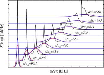
Figure 1: Comparison of the CBF $S(k,\omega)$ (black line), the CBF $S(k,\omega)$ folded with the instrumental resolution functions of Ref. Papp et al., 2008 (red line), and the Feynman approximation also folded with these functions (blue line) for soft spheres potential with the radius $R=3.5a$. Notice that the curves have been artificially shifted for clarity.

The analysis of the line shift experiments requires a theoretical model for $S(k,\omega)$ that allows finding the spectrum of elementary excitations. A suitable choice for that is provided by the Correlated Basis Function (CBF) method Chang and Campbell (1976), which is very well suited to describe weakly interacting Bose gasesApaja et al. (1997) and yields reasonable results also for ⁴He. We have found, however, that due to poor instrumental resolution, the detailed structure of $S(k,\omega)$ is washed out in the experiments and that the elementary excitation spectrum is very well described by the Feynman approximation. This is seen in Fig. 1, which shows a CBF calculation for a system of bosons interacting through the soft spheres potential $V(r\leq R)=V_{0},V(r>R)=0$ for $R=3.5$ in scattering length units. We have found that this simple model describes fairly well the experimental line shiftsPapp et al. (2008). The figure also shows the CBF $S(k,\omega)$ and the Feynman approximation, both folded with the instrumental resolution function of the experiments. The maxima of these broadened distributions agree very well and we conclude that the relevant quantity describing the dynamics in the experiment is $S(k)$.

We model the gas of $N$ ⁸⁵Rb atoms of mass $m$ with the Hamiltonian

$$H=-{\hbar^{2}\over 2m}\sum_{j=1}^{N}\nabla^{2}_{j}+\sum_{1=i<j}^{N}V(r_{ij})\mbox{{\bf{,}}}$$ (3)

and the ground state many-body wave function

$$\Psi_{0}({\bf r}_{1},{\bf r}_{2},\ldots,{\bf r}_{N})=\prod_{1=i<j}^{N}f(|{\bf r}_{i}-{\bf r}_{j}|)$$ (4)

is defined as a product of two–body correlation functionsFeenberg (1969), The unknown correlation function $f(r)$ is the solution of the variational problem which minimizes the expectation value of the Hamiltonian. With diagrammatic techniques the resulting Euler-Lagrange equation can be written in a Bogoliubov–like form for the structure function $S(k)$ Krotscheck (1986), which in scattering length units becomes

$$S(k)=\frac{k}{\sqrt{k^{2}+2\tilde{V}_{\rm p-h}(k)}}\,.$$ (5)

The effective, many-body potential in coordinate space splits into two parts,

$$V_{p-h}(r) = V(r)+$$

$$+ \left[g(r)-1\right]\left[w_{\rm ind}(r)+V(r)\right]+2\left(\nabla\sqrt{g(r)}\right)^{2}\,.$$

The potential on the first line is just the bare two-body potential. In momentum space

$$\tilde{V}(k)=\frac{4\pi^{2}x}{k}\int rdrV(r)\sin(kr)$$ (7)

defines the uniform limit approximation (with $\tilde{V}_{p-h}(k)=\tilde{V}(k)$)Feenberg (1969); Smith et al. (1979) for $S(k)$, that reduces in turn to the ordinary Bogoliubov expression when $V(r)$ is further approximated by the pseudopotential. The rest of the terms in Eq. (Elementary Excitations in Bose-Einstein Condensates at Large Scattering Lengths) contain the many-body contributions to the effective interaction. The radial distribution function $g(r)$ is calculated from the inverse Fourier transform

$$g(r)-1=\frac{1}{2\pi^{2}xr}\int kdk(S(k)-1)\sin(kr).$$ (8)

and the induced potential $w_{\rm ind}(r)$ is obtained by taking the inverse Fourier transform of the expression

$$\tilde{w}_{\rm ind}(k)=-\frac{1}{2}\left(2S(k)+1\right)\left(1-\frac{1}{S(k)}\right)^{2}\,.$$ (9)

Eqs. (5)-(9) form a set of self-consistent equations that have to be solved iteratively.

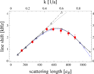
Figure 2: The line shift $\Delta\omega(k)$ as a function of the scattering length calculated using the PTGT (solid line) and SW (dashed line) potentials. Theoretical results are compared with the experimental points with error bars of Ref. Papp et al., 2008. Also shown are the hard sphere (dashed-dotted curve) and the pseudopotential (dotted curve) results. The upper axis shows $ka$ for a momentum $4\pi/780\,$nm^-1.

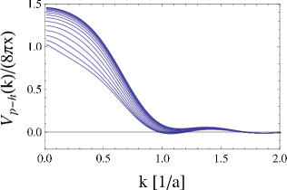
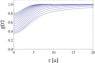
Figure 3: In the upper panel the effective many-body potentials as a function of momentum are shown for the PTGT-potential and different values of the scattering ength ranging from 100$a_{B}$ to 1500$a_{B}$ with 100$a_{B}$ steps. The lowest curve is for the lowest value of $a$ and the highest curve is equal to the Fourier transform of the bare two-body potential $\tilde{V}(k)$. The lower panel shows the radial distribution functions calculated using the PTGT-potential for the same values of the scattering length $a$. The lowest curve is for the lowest value of $a$.

A measure of the strength of the correlations in a quantum system is given by the amount $g(r)$ deviates from unity. From Eq. (Elementary Excitations in Bose-Einstein Condensates at Large Scattering Lengths) we see that many-body effects diminish when $g(r)\rightarrow 1$. That happens when $x$ increases for any potential with a Fourier transform as shown by Eqs. (8) and (7) provided that $S(k)$ has no singularities. For the PTGT-potential we find $V_{p-h}(k)\approx V(k)$ for $x\gtrsim 0.02$.

In the long wave length limit

$$\tilde{V}_{\rm p-h}(k=0)=mc^{2}\left(\frac{2ma^{2}}{\hbar^{2}}\right)\ ,$$ (10)

where $c$ is the speed of sound. At small $x$, i.e. $x<10^{-3}$, one recovers the pseudopotential result $\tilde{V}_{\rm p-h}(0)=8\pi x$. The agreement with Monte Carlo simulations S.Giorgini et al. (1999) is very good up to $x\approx 0.1$ even for the hard spheresMazzanti et al. (2003). For soft-core type potentials, the agreement should be even better at large $x$, because many-body contributions to $V_{p-h}(k)$ become less important.

We use two models for the single channel potential. The first one is the Poschl-Teller potential to which we have added a weak, attractive, Gaussian tail (PTGT). The attractive tail mimics the long range part of the van der Waals interaction, and it improves the fit to the experimental line shifts,

$$V(r)=\frac{G_{1}}{\cosh^{2}(\mu r)}-G_{2}e^{-\alpha(r-r_{0})^{2}}\,,$$ (11)

where $G_{1}=0.306038$, $G_{2}=0.012955$, $r_{0}=7.377861$, $\mu=0.383580$, and $\alpha=4.799\mu^{2}$. The second model in our analysis is the step-well potential (SW)

$$V(r)=\left\{\begin{array}[]{ll}V_{1},&\,\,\,\,\,\,r<R_{1}\\ -V_{2}&\,\,\,\,\,R_{1}<r<R_{2}\\ 0&\,\,\,\,\,r>R_{2}\end{array}\right.$$ (12)

with $V_{1}=0.110786$, $V_{2}=0.010572$, $R_{1}=4.684541$ and $R_{2}=1.5R_{1}$. All parameters are in scattering length units. They are fixed by setting the effective range $r_{\rm eff}/a\ll 1$, based on the multichannel scattering analysis near the Feshbach resonance by Bruun et al. Bruun et al. (2005) and by fitting the line shift data.

In Fig. 2 we compare our results to experiments. Up to $a=400a_{0}$ the behavior is almost linear and also both the pseudopotential and the hard sphere models fit well with the experimental data. Those models, though, are unable to reproduce the strong downwards bending observed in the line shifts at higher values of the scattering length.

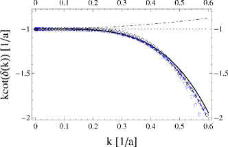
Figure 4: The effective range function as a function of the two-body scattering momentum for the PTGT (diamonds) and SW (circles) potentials. Least square fits are done for the range $0<k<0.5$ to the PTGT (solid curve) and SW (dashed curve) potentials. Also shown are the results for the hard sphere (dashed-dotted curve) and $\delta$-function (dotted curve) potentials.

The effective interaction $\tilde{V}_{\rm p-h}(k)$ determines the line shifts completely within the resolution of the experiments. In Fig. 3a we show its behavior for different values of the scattering length ranging from 100$a_{B}$ to 1500$a_{B}$ with 100$a_{B}$ steps using the PTGT-potential of Eq. (11). Since we have fixed the density to the experimental value, that range corresponds to $10^{-5}<x<0.04$ in the gas parameter. In the figure we have divided out the Bogoliubov constant $8\pi x$ and that is why at $k=0$ the lowest curve is very close to unity. Increasing the scattering length increases the strength of the potential at $k=0$ since the speed of sound increases (see Eq. (10)). The upper curves at the largest values of $a$ converge nicely to the Fourier transform of the bare potential. This means that many-body effects in $V_{p-h}(k)$ vanish and therefore the largest values available in experiments directly test the Fourier transform of the effective, bare potential. As long as the system remains in the gaseous phase, the particle–hole potential is directly given by the bare potential even if one keeps increasing $a$.

The momentum transfer fixed in the experiments varies in $1/a$-units from 0.13 to 0.76 as depicted in Fig. 2. Clearly understanding the behavior of the effective interaction as a function of the momentum transfer is essential since at $ka\approx 1$ the effective potential approaches zero defining an inverse healing distance $\xi^{-1}$ where the line shift should also go to zero.

The potential models chosen in Eqs. (11) and (12) give very similar line shifts within the experimental range, but at larger $a$ they behave very differently. Oscillations evident in the Fourier transform of the SW potential make it go through zero at $ka\approx 0.95$ whereas the PTGT-potential remains positive up to $ka\leq 1.7$. That difference could be experimentally tested by increasing the used momentum transfer by $\sim$20%. The SW potential also leads to the density wave instability at $a\approx 2260a_{B}$ with $ka=1.15$ whereas with the PTGT-potential the system remains in the gaseous phase. It could also be interesting to search for that phase transition experimentally.

In order to better understand the importance of the correlations we have plotted in Fig. 3b the radial distribution function $g(r)$ of the PTGT-potential for scattering lengths spanning the range $100a_{B}<a<1500a_{B}$. It shows that correlations diminish with increasing scattering length. That is why the effective potential $\tilde{V}_{\rm p-h}(k)$ is completely determined by the bare two-body potential at large $a$. In some sense that is equivalent to the behavior of the charged Bose gas Apaja et al. (1997) where the high density limit is the weakly correlated fluid.

In comparison of different models we plot in Fig. 4 the s-wave effective range function $k\cot(\delta_{0}(k))$ defined by the on-shell T-matrix for the different models used. At small $k<0.25$ it is very close to -1 supporting the scattering length approximation. At larger $k$ our model potentials give very similar downward bending. At $k>0.6$ the first order Born approximation becomes very accurate and we can conclude that the Fourier transform of the bare two-body potential $\tilde{V}(k)$, determines completely the large $k$ behavior of the effective range function. On the other hand, $\tilde{V}_{p-h}(k)$ for these momenta is also accurately determined by $\tilde{V}(k)$. This is not surprising since at large momenta the physics is governed by the short-distance two-body problem. This means that at large scattering lengths $\tilde{V}(k)$ could be determined by the line shift measurements. In Fig. 4 we also plot the hard sphere potential result and as shown it bends to the wrong direction. One can understand the link between $\tilde{V}_{p-h}(k)$ and the T-matrix by realizing that the large $k$ behaviour of both quantities is determined by the 2-body physics at short distances

Finally we give a simple parametrization by making a least square fit to the calculated effective range functions with a fourth degree polynomial

$$k\cot(\delta_{0}(k))=-1+\frac{1}{2}r_{\rm eff}k^{2}+Pk^{4}$$ (13)

when $0<k<0.5$. The $k^{4}$ coefficient is the shape parameter $P$, which turns out to be important for reproducing well the bending of the line shift at large $a$. With the PTGT-potential we find $P=-7.28$ and with the SW-potential $P=-7.88$. The quality of the polynomial fits is also show in Fig. 4.

In summary, we have assumed that the effective two-body potential scales with the scattering length and has a Fourier transform. Within these assumptions many-body correlations diminish with increasing scattering length and line shift experiments could be used to measure directly the Fourier transform of the bare two-body effective potential. The downward bending of the line shift clearly shows that effective interactions with finite strength and range are needed. By slightly increasing the gas parameter and momentum transfer one could study experimentally the formation of a possible density wave instability and by increasing the experimental resolution one could separate the elementary excitation mode from the continuum of multiphonon contributions as seen in ⁴He and the charged Bose gas.

We thank V. Apaja, G. Astrakharchik, J. Boronat and A. Polls for discussions. One of us (R. S.) thanks the Finnish Cultural Foundation and Vaisala fund for financial support. This work has been partially supported by Grant No. FIS2008-0443.

References

- Stamper-Kum et al. (1999) D. M. Stamper-Kum, A. P. Chikkatur, A. Gorlitz, S. Inouye, S. Gupta, D. E. Pritchard, and W. Ketterle, Phys. Rev. Lett 83, 2876 (1999).
- Steinhauer et al. (2002) J. Steinhauer, R. Ozeri, N. Katz, and N. Davidson, Phys.Rev. Lett. 88, 120407 (2002).
- Ozeri et al. (2005) R. Ozeri, N. Katz, J. Steinhauer, and N. Davidson, Rev. Mod. Phys. 77, 187 (2005).
- P.T.Ernst et al. (2009) P.T.Ernst, S.Götze, J.S.Krauser, K.Pyka, D-S.Lühmann, D.Pfankuche, and K.Sengstock, Nat. Phys. (2009), published online http://dx.doi.org/10.1038/nphys1505.
- Papp et al. (2008) S. B. Papp, J. M. Pino, R. J. Wild, S. Rosen, C. E. Wieman, D. S. Jin, and E. A. Cornell, Phys.Rev. Lett. 101, 135301 (2008).
- Feenberg (1969) E. Feenberg, Theory of Quantum Fluids (Academic, New York, 1969).
- Apaja et al. (1997) V. Apaja, J. Halinen, V. Halonen, E. Krotscheck, and M. Saarela, Phys. Rev. B 55, 12925 (1997).
- Krotscheck (1986) E. Krotscheck, Phys. Rev. B 33, 3158 (1986).
- Chang and Campbell (1976) C. C. Chang and C. E. Campbell, Phys. Rev. B 13, 3779 (1976).
- Smith et al. (1979) R. A. Smith, A. Kallio, M. Pouskari, and P. Toropainen, Nucl. Phys. A 328, 186 (1979).
- S.Giorgini et al. (1999) S.Giorgini, J.Boronat, and J.Casulleras, Phys.Rev. A 60, 5129 (1999).
- Mazzanti et al. (2003) F. Mazzanti, A.Polls, and A.Fabrocini, Phys.Rev. A 67, 063615 (2003).
- Bruun et al. (2005) G. M. Bruun, A. D. Jackson, and E. E.Kolomeitsev, Phys. Rev. A 71, 052713 (2005).