Large N and confining flux tubes as strings
– a view from the lattice

Abstract

I begin these three lectures by describing some of the useful things that we have learned about large-$N$ gauge theories using lattice simulations. For example that the theory is confining in that limit, that for many quantities SU(3) $\simeq$ SU($\infty$), and that this includes the strongly coupled gluon plasma just above $T_{c}$, thus providing some of the justification needed to make use of gauge-gravity duality in analysing QCD at RHIC/LHC temperatures. I then turn, in a more detailed discussion, to recent progress on the problem of what effective string theory describes confining flux tubes. I describe lattice calculations of the energy spectrum of closed loops of confining flux, and some dramatic analytic progress in extending the ‘universal Luscher correction’ to terms that are of higher order in $1/l^{2}$, where $l$ is the length of the string. Both approaches point increasingly to the Nambu-Goto free string theory as being the appropriate starting point for describing string-like degrees of freedom in SU($N$) gauge theories.

11.15.-q, 11.15.-Pg, 11.15.Ha, 11.25.Pm

1 Introduction

Over the last ten years lattice simulations have helped us learn a great deal about ’t Hooft’s large-$N$ limit of gauge theories and QCD. This resurgence of interest on the lattice side [1] coincided (co-incidentally) with the culmination of the ‘second superstring revolution’ in Maldacena’s AdS/CFT correspondence [2] and the gauge-gravity dualities that have flowed from it. These dualities between weakly coupled string theories and strongly coupled gauge theories at large $N$, have led to a common interest in what is the physics of large $N$ gauge theories.

At the same time, Maldacena’s work has provided a new and unexpected twist to the very old question of what, if any, string theory describes the strong interactions and hence gauge theories. A narrower version of this question is to ask what effective string theory describes the dynamics of confining flux tubes in gauge theories. Certainly at large $N$ this latter question, when applied to long flux tubes and to their low-lying excitations, should become entirely well-defined. Any answer promises to provide essential insights into what might be the answer to the first and much more speculative question.

I begin these lectures with some cursory remarks about the large $N$ limit (with which I assume you are all familiar) and I then give you an overview of how one does lattice calculations, describing how one can obtain predictions for interesting physical quantities, such as ratios of masses, in the continuum gauge theory. In Section 3 I select a few topics about large $N$ gauge theories that have been addressed (and largely resolved) by lattice calculations in recent years. Is SU($\infty$) linearly confining? Is SU(3) close to SU($\infty$)? Is QCD close to QCD_∞? How does the coupling run, and should we keep $g^{2}N$ fixed for a smooth large-$N$ limit? I finish this Section by discussing how the computational cost increases with $N$, and show that large-$N$ calculations are surprisingly inexpensive and accessible. I then devote Section 4 to discussing large $N$ gauge theories at finite temperature; in particular above but not too far from the deconfining transition. This is of particular interest since it has become the focus of a large AdS/CFT effort in recent years. Section 5 is very brief and just lists some topics on which there has been interesting work, but which I have no time to discuss in these lectures. The remainder of my lectures is devoted to my second topic: what is the effective string theory that describes confining flux tubes. Section 6 summarises the analytic work that has accompanied and motivated (and been motivated by) the large amount of numerical work on this question that has been carried out over the last three decades. After some general background, and a detailed description of both the Gaussian approximation and the Nambu-Goto free string theory, I describe the dramatic progress that has been achieved in the last five years (with some startling papers appearing even as I write these lectures). I finish the Section with a potted and inadequate history of numerical calculations during this period. I then move on to the numerical calculations of the energy spectrum of closed flux tubes that I have been involved in for the last 4 or 5 years. Section 7 discusses our calculations in SU($N$) gauge theories in $2+1$ dimensions. We obtain very accurate energy estimates for quite a large number of low-lying eigenmodes, and I display how remarkably well Nambu-Goto describes these even when the flux tube is so short that it is hardly longer than it is wide. In Section 8 I give a brief preview of our unpublished work on SU($N$) gauge theories in $3+1$ dimensions. Here there is an interesting distinction between the majority of states, which adhere closely to a Nambu-Goto-like spectrum, much as in $D=2+1$, and a significant minority of states that behave quite differently. I will finish, in Section 9, with some concluding remarks, although the bulk of my conclusions are embedded, at appropriate points, in these lectures.

2 Preliminaries

2.1 Large $N$

In $D=3+1$ gauge theories one has a dimensionless coupling $g^{2}$ and one might hope to be able to use it as a general expansion parameter for the theory. However because the scale invariance is anomalous, setting $g^{2}$ to some particular value $g_{0}^{2}$ means that we can only hope to use it as a useful expansion parameter for physics close to the scale $l_{0}$ where the running coupling takes that value, i.e. where $g^{2}(l=l_{0})\simeq g_{0}^{2}$. In $D=2+1$ gauge theories $g^{2}$ has dimensions of mass so that the dimensionless expansion parameter for physics on the scale $l$ is $g^{2}l$ and one immediately sees that the coupling cannot serve as a useful expansion parameter for the theory as a whole.

Faced with this, ’t Hooft suggested, back in 1974 [3], that an alternative, less obvious but more general expansion parameter might be provided by $1/N$. That is to say one thinks of expanding SU($N$) gauge theories in powers of $1/N^{2}$ around SU($\infty$). Pictorially:

$$SU(N)=SU(\infty)+O\left(\frac{1}{N^{2}}\right).$$ (1)

That the expansion parameter is $1/N^{2}$, follows from ’t Hooft’s analysis of all-order perturbation theory using his clever double-line notation for gluon propagators and vertices, in which the gluon is represented by a fundamental line and its conjugate. (For simplicity I will here ignore the difference between U($N$) and SU($N$).) It also follows that a smooth large-$N$ limit can only be achieved if one keeps $g^{2}N$ fixed. We can begin to see why this should be so by considering a gluon loop insertion in the gluon propagator using the double-line notation, as shown in Fig. 1. The two vertices give a factor of $g^{2}$ and the sum over the colour index in the closed loop gives a factor of $N$. So such an insertion produces a factor of $g^{2}N$ in the amplitude. If we want smooth physics as $N\to\infty$, then at the very least we require that the number of such insertions, in the dominant diagrams contributing to the physics of interest, should be roughly fixed as we vary $N$. This requires that we keep $g^{2}N$ fixed in that limit. One can readily generalise the argument to all diagrams.

This argument looks perturbative, but it is nonetheless convincing because in demanding that there is a smooth large-$N$ limit, we are demanding inter alia that SU($\infty$) should be asymptotically free. If instead of keeping $g^{2}N$ fixed we vary $g^{2}\propto 1/N^{1+\epsilon}$ with $\epsilon<0$ it is clear that at $N=\infty$ infinite order diagrams will dominate at any scale where we attempt to apply perturbation theory, i.e. there is no asymptotic freedom. If on the other hand we take $\epsilon>0$, one would be driven to a free theory on any scale where one attempts to apply perturbation theory. Neither result is what we want, so the only limit that can work is to keep $g^{2}N$ fixed as $N\to\infty$. Note however that while we can easily argue this condition to be necessary, there is no guarantee that it is sufficient.

Figure 1: Gluon loop insertion using ’t Hooft’s double line notation.

In the gauge theory the coupling runs, so a little care is needed in defining what we mean by keeping $g^{2}N$ fixed. So first let us define the length scale for the running coupling in units of say the mass gap, i.e. $lm_{G}$. Then define the ’t Hooft coupling $\lambda_{N}=g^{2}N$ for the SU($N$) gauge theory. Then the appropriate way to encode $g^{2}N=\mathrm{const}$ is simply as follows:

$$\lambda_{N}(lm_{G})\longrightarrow\lambda_{\infty}(lm_{G})$$ (2)

i.e. the ’t Hooft coupling on a scale $l$, where the scale $l$ itself is fixed in physical units, tends to a non-trivial limit as we sweep through the various SU($N$) gauge theories.

The large-$N$ expansion will only be useful if the theory we are expanding about, SU($\infty$), is sufficiently simple. Although it is, in fact, not so simple that we can solve it analytically, some things are very simple in a large-$N$ confining phase [4]. This essentially arises because the probability of any quarks or gluons forming a colour singlet (rather than some other representation) goes to zero as the number of colours increases. This, together with the fact that $g^{2}\propto 1/N\to 0$ is the reason that we have zero decay widths, zero mixing, a perfect OZI rule and no colour singlet scattering in that limit.

Of course it would be nice to show that there is in fact a large $N$ confining phase, and that a smooth physics limit does in fact exist. And we would like to determine what precisely that physics is. And we would like to check whether, for at least some reasonably wide class of important physical quantities, we can say that SU(3) (and $QCD$) are indeed close to SU($\infty$) (and $QCD_{N=\infty}$). This is after all the reason many of us might be interested in the large-$N$ limit. At present these questions can only be addressed numerically.

Before moving on to these numerical calculations, let me emphasise that there is no expectation that all the physics of SU(3) is close to that of SU($\infty$). Indeed it is clear that this cannot be so and in that sense eqn(1) is misleading. Indeed it is entirely possible that other large-$N$ limits may be more appropriate for some physics. For example, in QCD we have 2 or 3 light flavours, so $N_{f}/N\sim 1$. It might appear plausible that the limit $N\to\infty$ with $N_{f}/N$ fixed might be more appropriate for some physical quantities [5]. (Or a limit with fermions in the bi-fundamental representation [6] which has the virtue that some quantities become calculable at $N=\infty$ because the theory effectively has some supersymmetry in that limit.) However it is worth noting that the ’t Hooft limit has turned out to be phenomenologically useful even in some cases where one would naively have not expected it to be. A good example is the case of baryons, which consist of $N\to\infty$ quarks, but where one has inferred a useful SU(6)-like symmetry to describe the multiplet structure [7].

2.2 Lattice calculations [8]

We want to calculate correlation functions numerically. These can be expressed as Feynman path integrals. Generically:

$$Z=\int\prod_{x\in M_{4}}d\phi(x)e^{iS[\phi]}$$ (3)

After we explicitly integrate over any Grassmanian quark fields, the integrand depends just on ordinary numbers (which may be grouped into SU($N$) matrices) so one can imagine doing the integral numerically.

To be able to do this we first need to get rid of the phase factor $\exp\{iS\}$ since numerical integrations involving phase factors are notoriously ill conditioned (the sign problem). This we achieve (in the cases of interest in these lectures) by going to Euclidean space-time, so that $i\int dt\to\int dt$. (How that affects what we can calculate will be addressed in a moment.) The next problem is that we have an infinite number of integrations. For a numerical calculation this must be made finite: so the space-time volume must be made finite and discrete. It is usually convenient to use a hypertorus and a hypercubic lattice for these purposes. (Sometimes other choices are useful.) So these two steps look like:

$$\int\prod_{x\in M_{4}}d\phi(x)e^{iS[\phi]}\to\int\prod_{x\in R^{4}}d\phi(x)e^{-S_{E}[\phi]}\to\int\prod_{n\in T^{4}}d\phi_{L}(n)e^{-S_{L}[\phi_{L}]}$$ (4)

where we express the discrete space-time points as $x=na$ where $n$ is a $D$-tuple of integers, $a$ is the lattice spacing, and $\phi_{L}$ is a dimensionless lattice field variable, with action $S_{L}$, chosen so that

$$\phi_{L}(x) \stackrel{{\scriptstyle a\to 0}}{{\longrightarrow}} a^{-dim(\phi)}\phi(x)$$

$$S_{L} \stackrel{{\scriptstyle a\to 0}}{{\longrightarrow}} S_{E}$$ (5)

where $dim(\phi)$ is the length dimension of the field $\phi$. Obviously this schematic outline of the continuum limit misses many essential details.

Two asides. Firstly, putting the theory in a finite box of size $l$ can be harmless if, as here, the theory has a finite mass gap, $m_{G}$, because in such a case we expect finite-size effects to be $O(e^{-m_{G}l})$ which can easily be made very small by choosing $l\gg 1/m_{G}$. Secondly, since the theory is renormalisable, what we do at short distances, e.g. introducing a lattice cut-off, can be simply absorbed into the renormalisation of parameters such as the coupling, if we choose $a\ll 1/\Lambda$, where $\Lambda$ is the typical dynamical energy scale. Moreover since the theory is asymptotically free, we can analyse the lattice spacing corrections in a perturbation expansion in the small coupling $g^{2}(a)$.

The continuum degrees of freedom are the gauge potentials $A_{\mu}(x)$ which belong to the SU($N$) Lie algebra. They tell us how to compare colour at infintesimally neighbouring points. If we want to compare colour between points with a finite separation, we use the path ordered exponential of the gauge potential along some path $c$ joining the points: $P\exp\{i\int_{c}A.ds\}$. This is an SU($N$) group element which ‘lives on’ the particular path chosen. So the natural gauge degrees of freedom on the lattice, where all points are a finite distance apart, are group elements, $U_{l}$, that live on the links, $l$, of the lattice. More specifically, if the link goes from the site $x$ to the site $x+a\hat{\mu}$, we label this group element by $U_{\mu}(x)$. Under a gauge transformation $V(x)$, it is defined to transform as

$$U_{\mu}(x)\longrightarrow V(x)U_{\mu}(x)V^{\dagger}(x+a\hat{\mu})$$ (6)

as would the corresponding path ordered exponential in the continuum theory. To the same link but taken in the reverse direction, i.e. $x+a\hat{\mu}$ to $x$, we assign $U^{\dagger}_{\mu}(x)$. Thus if we go out along a link and then return by the same link to the same point, the colour comparison matrix is the unit matrix, as it should be.

We choose for our integration measure the standard Haar measure which has the nice property that it invariant under left or right multiplication and hence gauge invariant:

$$dU_{\mu}(x)=d\{V(x)U_{\mu}(x)V^{\dagger}(x+a\hat{\mu})\}.$$ (7)

Now all we need is a gauge-invariant action. It is easy to see that the trace of the product of link-matrices around any closed path $c$, $\mathrm{Tr}\prod_{l\in c}U_{l}$, is gauge invariant. (To any backward going link $l$ we assign $U^{\dagger}_{l}$.) Now, the continuum action compares fields at (infinitesimally separated) neighbouring points. We can compare neighbouring link matrices on a lattice by taking their product. To be gauge-invariant this product should appear within a product of matrices being taken around some closed path. The simplest and most common choice is to use the path that is an elementary square on the lattice, called a plaquette. So for the action we take

$$S=\sum_{p}\left\{1-\frac{1}{N}\mathrm{ReTr}U_{p}\right\}$$ (8)

where $U_{p}$ is the path-ordered product of link matrices around the plaquette $p$. The $\sum_{p}$ ensures that the action is translation and rotation invariant. Taking the real part of the trace ensures that it has $C=P=+$. So our lattice path integral is

$$Z=\int\prod_{l}dU_{l}e^{-\beta S}$$ (9)

where $\beta$ is any constant. It is the only free parameter in $Z$, so it is by varying $\beta$ that we will be able to vary the lattice spacing $a$. Since our lattice theory has the important continuum symmetries (albeit a subgroup for rotations and translations) we expect that in the continuum limit, barring an unnatural choice of lattice action (and here I mean unnatural in the technical sense as applied, for example, to a light Higgs scalar) we must obtain the continuum action, i.e.

$$\int\prod_{l}dU_{l}e^{-\beta S}\stackrel{{\scriptstyle a\to 0}}{{\longrightarrow}}\int\prod_{x,\mu}dA_{\mu}(x)e^{-\frac{4}{g^{2}}\int d^{4}xTrF_{\mu\nu}F_{\mu\nu}}$$ (10)

(up to a possibly infinite constant). This tells us that in the continuum limit $\beta=c/g^{2}$. A more careful analysis tells us what $c$ is:

$$\beta=\frac{2N}{g^{2}_{L}(a)}\qquad;\qquad g^{2}_{L}(a)\stackrel{{\scriptstyle a\to 0}}{{\longrightarrow}}g^{2}(a)$$ (11)

where $g^{2}_{L}(a)$ is a running coupling on the scale $a$ in (this particular) lattice coupling scheme, and $g^{2}(a)$ is a running coupling in a(ny) continuum scheme. (In this limit any difference between schemes is $O(g^{4})$.) Since $g^{2}(a)\to 0$ as $a\to 0$ we know how to find the continuum limit; one simply takes $\beta\to\infty$.

Although the above has been for $D=3+1$ dimensions, we can follow the same steps in $D=2+1$. In this case $g^{2}$ has dimensions $[m]$, so the dimensionless bare lattice coupling is $ag^{2}$ and, not surprisingly, we find

$$\beta=\frac{2N}{ag^{2}}\stackrel{{\scriptstyle a\to 0}}{{\longrightarrow}}\infty\qquad:D=2+1$$ (12)

where this $g^{2}$ becomes the $g^{2}$ of the continuum theory when $a\to 0$.

Suppose we want to calculate the expectation value of some functional $\Phi[U]$ of the gauge fields. We generate a set of $n$ gauge fields $\{U^{I}\};I=1,...,n$ distributed not just with the measure $\prod_{l}dU_{l}$, but with the Boltzmann-like action factor included, i.e. as $\prod_{l}dU_{l}\exp\{-\beta S[U]\}$. I won’t go into the details – there are standard heat bath, Metropolis and HMC algorithms available. We thus obtain:

$$\langle\Phi\rangle=\frac{1}{Z}\int\prod_{l}dU_{l}\Phi[U]e^{-\beta S}=\frac{1}{n}\sum^{n}_{I=1}\Phi[U^{I}]+O\left(\frac{1}{\surd n}\right)$$ (13)

where the last term is the statistical error.

How, for example, should we calculate the mass gap? Recall the standard decomposition of a Euclidean correlator of some operator $\phi(t)$ in terms of the energy eigenstates:

$$\langle\phi^{\dagger}(t=an_{t})\phi(0)\rangle = \langle\phi^{\dagger}e^{-Han_{t}}\phi\rangle=\sum_{i}|c_{i}|^{2}e^{-aE_{i}n_{t}}$$ (14)

$$\stackrel{{\scriptstyle t\to\infty}}{{=}} |c_{0}|^{2}e^{-am_{0}n_{t}}$$

where the lightest mass is $m_{0}$ and its exponential falls slowest with $t$ and hence will dominate at large $t$, as shown. Note that the only states that can contribute are those that have $c_{j}=\langle vac|\phi^{\dagger}|j\rangle\neq 0$, so we should match the quantum numbers of the operator $\phi$ to those of the state we are interested in. So typically we construct a $\phi$ with the desired $J^{PC}$ quantum numbers, and if we are interested in masses we also make $\phi$ have $\vec{p}=0$. Note also that because what we know is the value of $n_{t}$, we will always obtain the mass in lattice units, i.e as $am_{0}$, when we fit our numerical ‘data’ with an exponential in $n_{t}$.

So, having decided on a suitable operator $\phi$, we calculate it as in eqn(13) with $\Phi=\phi^{\dagger}(t)\phi(0)$. This will produce an estimate of $\langle\phi^{\dagger}(t)\phi(0)\rangle$ with a finite statistical error. To extract a value of $am_{0}$, using eqn(14), we clearly need to have significant evidence for the exponential behaviour $\propto e^{-am_{0}n_{t}}$, over some range of $n_{t}$, and this range needs to be at small enough $n_{t}$ that the exponential is still clearly visible above the statistical errors. This is obviously harder to achieve for larger $m_{0}$, so the systematic error will be larger for heavier states. However, even for the lighter states we need the (normalised) $|c_{0}|^{2}\simeq 1$: our operator needs to be a good wavefunctional for the state whose energy we are interested in, so that its correlator is dominated by this state even at small $n_{t}$.

Let us now have an explicit example of how to calculate the lightest $0^{++}$ glueball mass in the $D=3+1$ SU(3) gauge theory. Our space-time is a $32^{4}$ hypercubic lattice with periodic boundary conditions (i.e. a hypertorus). We use a Monte Carlo to generate typical lattice gauge fields at $\beta=6/g^{2}=6.515$. Once we calculate the string tension we will find that this corresponds to $a\surd\sigma\simeq 0.101$ i.e. $a\simeq 0.05\mathrm{fm}$ if we use the conventional value of $\surd\sigma\sim 0.5\mathrm{fm}$. So the lattice spacing is very small and we are close to the continuum limit.

As a first attempt, we shall try the simplest operator we can think of, i.e. one that is based on the plaquette that appears in our lattice action:

$$\phi_{p}(t)=\sum_{\vec{x}}\sum^{3}_{\mu,\nu=1}\mathrm{ReTr}U_{\mu\nu}(\vec{x},t)$$ (15)

where $U_{\mu\nu}(x)$ is the product of link-matrices around the boundary of an elementary square $p$ in the ${\mu\nu}$ plane emanating out of the site $x$ (in the directions that have been chosen as positive). This operator clearly has, as desired, $\vec{p}=0$ and $J^{PC}=0^{++}$, since it is explicitly translation and rotation invariant. However it also has a non-zero overlap onto the vacuum, so we shall use the shifted operator $\phi_{p}(t)\longrightarrow\phi_{p}(t)-\langle\phi_{p}\rangle$ so as to prevent the vacuum from appearing in the sum over energy eigenstates in eqn(14). The numerical result for the correlation function (based on about 100,000 Monte-Carlo generated gauge fields) is shown in Fig. 2. This result is clearly disappointing. Only for $n_{t}=0,1,2$ are the errors small enough for $C(n_{t})$ to be useful. And we cannot put a simple exponential through these 3 points, although we can do so trivially for the $n_{t}=1,2$ points as shown in Fig. 2. That is to say we have no evidence that the lightest state dominates this correlation function and we are unable to extract a mass for the lightest state.

Figure 2: Glueball correlation function with a simple plaquette operator.

The problem is that the plaquette is so local that it does not see the structure of a wave-function and will therefore have a roughly equal overlap onto all the eigenstates. Since the number of excited states increases rapidly with decreasing $a$, the (normalised) overlap onto the groundstate will decrease rapidly. At the small value of $a$ at which we are here working, this overlap is presumably very small and we would have to go to quite large $t=an_{t}$ to suppress the excited states and reveal the ground state. Looking at the errors in Fig. 2, and taking into account that this is based on $O(10^{5})$ lattice fields, this is clearly unrealistic. So what we need are operators that are ‘smooth’ on a scale $\sim 1\mathrm{fm}$ and which will therefore have very little overlap onto the ‘oscillating’ wavefunctions of excited states. Note that simple Wilson loops that are merely larger than the plaquette will in general not be sufficient. We need Wilson loops that are densely packed within a volume $\sim 1\mathrm{fm}$ (like a ‘ball of wool’). We can efficiently construct such operators that are ‘smooth’ on physical length scales, by the iterative spatial ‘smearing’ [9] and ‘blocking’ [10] of the lattice gauge fields. (This essentially consists of summing over several paths between two sites, projecting the sum back into the group, and calling this a smeared link. And then iterating the procedure.) We can then use these ‘blocked’ link matrices to construct appropriate Wilson loops that will be summed as in eqn(15) to produce corresponding operators. Using different Wilson loops and different iteration levels of the blocking will thus produce some set $\{\phi_{i};i=1,...,n\}$ of operators of the desired quantum numbers. Linear combinations of these operators form a vector space $V_{\phi}$, and we can perform a variational calculation to obtain our best estimate, $\psi_{0}$, of the ground state operator [11, 12, 13]:

$$\langle{\psi_{0}}^{\dagger}(t_{0})\psi_{0}(0)\rangle=\max_{\phi\in V_{\phi}}\langle\phi^{\dagger}(t_{0})\phi(0)\rangle=\max_{\phi\in V_{\phi}}\langle\phi^{\dagger}e^{-Ht_{0}}\phi\rangle$$ (16)

where $t_{0}$ is some convenient value of $t$. Then $\psi_{0}$ is our best variational estimate for the true eigenfunctional of the ground state (with these quantum numbers) and we can now use the correlator $\langle{\psi_{0}}^{\dagger}(t)\psi_{0}(0)\rangle$ to obtain our best estimate of the ground state mass. This generalises in an obvious way to calculating excited state energies. One constructs from $V_{\phi}$ the vector space orthogonal to $\psi_{0}$, repeats the above within this reduced vector space, and obtains $\psi_{1}$ which is our best variational estimate for the true eigenfunctional of the first excited state. And so on.

If we do this in our present example we get the ground state correlation function shown in Fig. 3. This can be fitted with a single exponential (or rather a cosh because of the periodicity in $t$) over a large range of $n_{t}$ values where $C(n_{t})$ is accurately determined. (We cannot include $n_{t}=0$ with a good $\chi^{2}$, and in fact the overlap factor is $|c_{0}^{2}|\simeq 0.97$.) From the fit we obtain an estimate of $am_{0^{++}}=0.330(7)$ for the lightest scalar glueball mass. It turns out that this is the lightest mass tout court – it is the mass gap of the SU(3) gauge theory. The reassuring point is that we are able to calculate masses numerically with errors that are at the percent level. This means that we will be able to perform meaningful continuum extrapolations.

Figure 3: Glueball correlation function with best blocked operator and cosh fit.

To obtain the continuum limit from masses that are in lattice units and are distorted by the finite lattice cutoff, we take dimensionless ratios of masses, to get rid of lattice units, and then extrapolate these ratios to $a=0$ with an $O(a^{2})$ lattice correction, which is what is appropriate for a pure-gauge plaquette action [14], e.g.

$$\frac{am(a)}{a\surd\sigma(a)}=\frac{m(a)}{\surd\sigma(a)}=\frac{m(0)}{\surd\sigma(0)}+c_{0}a^{2}\sigma+O(a^{4}).$$ (17)

Here we choose to use the square root of the string tension $a^{2}\sigma$ as one of the masses, but we could just as well have chosen some other glueball mass. (Aside: here $c_{0}$ is in fact a power series in the bare coupling, but the logarithmic variation with $a$ is weak and can usually be ignored within the errors of current calculations. This will not remain so for ever.) To do such an extrapolation we need to perform the mass calculations at several values of $\beta$. Doing so for the lightest $0^{++}$ and $2^{++}$ glueball masses, we obtain the results displayed in Fig. 4. I show there the linear $O(a^{2})$ extrapolations to the continuum limit, $a^{2}\sigma=0$. Clearly they are well-determined by these numerically determined mass ratios. We obtain

$$\frac{m_{0^{++}}}{\surd\sigma}=3.47(4)-5.52(75)a^{2}\sigma$$ (18)

for the mass gap, and $m_{2^{++}}/\surd\sigma=4.93(5)-0.61(1.36)a^{2}\sigma$ for the lightest tensor. (Errors statistical only.) In the continuum limit we thus obtain

$$m_{0^{++}}\simeq 3.5\surd\sigma\simeq 1.6\ {\mathrm{GeV}}.$$ (19)

This now quite old lattice prediction [15], has helped to motivate the now popular phenomenological interpretation (e.g. [16]) of the three observed $J^{PC}=0^{++}$ flavour ’singlet’ states, the $f_{0}(1350),f_{0}(1500)$ and $f_{0}(1700)$, as arising from the mixing of nearby $u\overline{u}+d\overline{d}$, $s\overline{s}$ and glueball states.

Figure 4: Scalar, $\bullet$, and tensor, $\circ$, glueball masses with $O(a^{2})$ extrapolations to the continuum limit.

For our purposes here, the important point is that we are able to calculate mass ratios in the continuum gauge theory at the percent level of accuracy. This means that we should have the necessary accuracy to compare physical mass ratios in different SU($N$) gauge theories, and to extrapolate to $N=\infty$.

3 Large $N$ Physics : some basic results from the lattice

If the large-$N$ expansion is to be useful for understanding the strong interactions, the SU($N\to\infty$) gauge theory needs to be confining at low temperatures, $T$, and at least some of the physics needs to be very similar to that of the SU(3) theory. This is what we will seek to establish in the first part of this section. I shall then describe some recent calculations that include quarks, and which begin to address the question whether the mesonic spectrum of $QCD$ is ‘close to’ $QCD_{N=\infty}$. Finally I will return to the question of how one should take a smooth large-$N$ limit : do our non-perturbative calculations support the diagrammatic expectation that you hold $g^{2}N$ fixed?

Our method is simple. We calculate physical mass ratios first for SU(2), then for SU(3), then for SU(4), …, and continue for larger groups until we have good evidence that our results are indeed converging to a large-$N$ limit with the expected leading $O(1/N^{2})$ corrections. This method is pedestrian but effective.

I shall finish with some remarks about how the cost of the calculations grow with $N$. In fact the growth is unexpectedly modest in many situations – which I hope will encourage some of you to get actively involved.

3.1 Are large-$N$ gauge theories linearly confining?

I will answer this question first by example and then, later on, more quantitatively.

The example is taken from SU(6) in $D=3+1$ [17]. We calculate the mass of the lightest state in which one unit of fundamental flux closes upon itself by winding once around a spatial torus. Suppose this torus is of length $l$. Then if we have linear confinement the flux will organise itself into a flux tube (of the same kind as would join two distant fundamental sources) and the mass will grow linearly with $l$ for large $l$, $m(l)\stackrel{{\scriptstyle l\to\infty}}{{=}}\sigma l$. How you actually do this and what operators you need to use, will be discussed in some detail later on in these lectures.

Figure 5: Ground state energy of a flux loop winding around a spatial torus of length $l$, in SU(6) and $D=3+1$.

The results of this calculation are shown in Fig. 5. It is immediately apparent from the plot that we do indeed have the (approximately) linear increase with $l$ that indicates linear confinement. So that you can judge what is the length $l$ in physical units, I have used the value of $a\surd\sigma$ from our fits to translate the lattice size $l=aL$ into physical units using $l\surd\sigma=aL\surd\sigma=L\times a\surd\sigma$. Since we expect the intrinsic width of a flux tube to be $O(1/\surd\sigma)$ we can see that our largest values of $l$ are indeed large compared to the flux tube width and it is reasonable to infer that what we are seeing is the onset of an asymptotic linear behaviour.

The dashed line shown on the plot represents a linear piece modified by the Luscher correction term

$$m(l)=\sigma l-\frac{\pi}{3l}.$$ (20)

This $O(1/l)$ correction is universal and the value used here corresponds to the universality class of a simple bosonic string where the only massless modes are those of the transverse oscillations. We can see from Fig. 5 that this correction captures the bulk of the observed deviation from linearity. (One of course expects further corrections that are higher powers of $1/l$.) So we have good evidence not only that linear confinement persists at large $N$, but that it remains in the same universality class as has been established by previous work for SU(2) and SU(3).

3.2 Is SU(3) close to SU($\infty$)?

In Fig. 3 we showed how to calculate a mass on the lattice, and in Fig. 4 how to obtain ratios of masses in the physical continuum limit of the theory. That example was for SU(3) but one can do the same for other values of $N$. In Fig. 6 I plot the resulting continuum ratios for $N=2,3,4,6,8$ [18]. Since the leading correction is expected to be $O(1/N^{2})$, I plot the ratios against $1/N^{2}$. In such a plot the large-$N$ extrapolation should be a simple straight line for large enough $N$. In practice, within our errors, large enough $N$ turns out to mean $N\geq 3$ (indeed, $N\geq 2$ for the scalar glueball) as we see from the linear fits on the plot. It is also evident that the coefficient of this $1/N^{2}$ term is typically quite modest (compared to the $N=\infty$ value of the ratio). Thus this provides an example of the fact that for many basic physical quantities

$$SU(3)\simeq SU(\infty).$$ (21)

Figure 6: Scalar, $\bullet$, and tensor, $\circ$, glueball masses in various continuum SU($N$) gauge theories, with $O(1/N^{2})$ extrapolations to $N=\infty$ limit.

There is something else that we can infer from Fig. 6. We provided evidence earlier on that linear confinement persists at large $N$. However it could still be that it disappears as $N\to\infty$ through $\sigma$ vanishing in that limit. What Fig. 6 demonstrates is that this is not the case. In units of the physical glueball masses $\sigma$ remains non-zero at $N=\infty$. (Logically, one should first show a plot of the ratio of the scalar to tensor masses in order to establish the existence of a smooth large $N$ limit, but it is clear from Fig. 6 that this is the case.)

3.3 Is $QCD_{3}$ close to $QCD_{\infty}$?

To estabish the phenomenological relevance of the large-$N$ limit we need to consider mesons as well as glueballs. Once we have fields in the fundamental representation, like quarks, we have $O(1/N)$ corrections. (A quark self-energy loop in the gluon propagator will look just like Fig. 1 except without the innermost closed loop and the accompanying factor of $N$ from the sum over colours.) Thus the fact that we see $SU(3)\sim SU(\infty)$ in the pure gauge theory, where the leading correction is $O(1/N^{2})$, does not guarantee that the meson spectrum will be so well-behaved. Whether it is needs to be checked, and there have been three recent calculations that have begun to do precisely that [19, 20, 21].

As $N\to\infty$ quark loops are suppressed by a factor $1/N$ compared to gluon loops, and so to leading order the vacuum of $QCD_{N=\infty}$ is the same as that of the SU($N$) gauge theory. (As long as the quarks are not precisely massless, when subtle issues arise.) We can of course still ask what happens to the spectrum of mesons at $N=\infty$, by explicitly calculating their propagators. When doing so we are calculating them in in what one would usually call the relativistic valence quark approximation except that here it is not an approximation, because the quark loops are not being neglected but are dynamically suppressed. (And in addition the gluonic vacuum in which the quarks propagate is the complete non-perturbative vacuum and not some crude approximation thereof.)

This suggests an efficient way to proceed. (A straightforward calculation of full $QCD_{N}$ with light quarks being too expensive.) At various finite $N$ one performs the meson spectrum calculation without vacuum quark loops – what is called the ‘quenched approximation’ in the lattice community. One then extrapolates the quenched results to $N=\infty$. Since we have no quark loops the leading correction should be $O(1/N^{2})$. The extrapolated values are the correct values for $QCD_{N=\infty}$ since that theory is dynamically quenched. We now compare the spectrum at $N=\infty$ with the experimental spectrum (or that of recent full lattice $QCD$ calculations, which indeed agree with experiment).

This looks like a win-win approach except for the fact that quenched QCD at finite $N$ is not unitary. However the pathologies are subtle and appear primarily at small quark masses, so if one extrapolates to $N=\infty$ at fixed non-zero quark masses and only then to small quark masses, one should be largely protected from them. Current calculations are not so pedantic, but since they are probably not accurate enough to be sensitive to such pathologies anyway, this does not really matter.

In Fig. 7 I show some plots borrowed from [19]. On the left is a plot of the $\rho$-meson mass against $m^{2}_{\pi}$ for $N=2,3,4,6$ and obtained at one value of $a\surd\sigma$ (chosen to be very similar for all the SU($N$) groups). Such a linear behaviour is what one expects if $m_{\rho}(m_{q})=m_{\rho}(0)+cm_{q}$ and $m^{2}_{\pi}\propto m_{q}$ (spontaneous chiral symmetry breaking). We see that there is very little variation with $N$. On the right is a plot of the chirally extrapolated $m_{\rho}(0)$ against $1/N^{2}$, which also shows little variation.

         

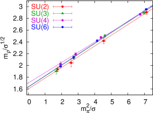
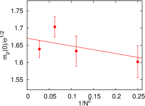
Figure 7: Left: the $\rho$ mass against $m^{2}_{\pi}$ for various SU($N$). Right: chiral extrapolation of $m_{\rho}$ for various $N$ and an $O(1/N^{2})$ extrapolation to $N=\infty$.

So at this particular value of $a$, corresponding to $a\sqrt{\sigma}=0.209$, one obtains $\lim_{N\to\infty}{m_{\rho}}/{\sqrt{\sigma}}=1.688(25)$. Now, fortunately there has been another calculation [20], with exactly the same lattice action, but at a different lattice spacing, $a\sqrt{\sigma}=0.335$, obtaining $\lim_{N\to\infty}{m_{\rho}}/{\sqrt{\sigma}}=1.627(10)$. This allows us to make an $O(a)$ continuum extrapolation. (Although with two points it is of course not under good control.) This gives a value [19],

$$\lim_{N\to\infty,a\to 0}\frac{m_{\rho}}{\sqrt{\sigma}}=1.79(5)$$ (22)

to be compared with the real world value of

$$\frac{m_{\rho}}{\sqrt{\sigma}}\simeq\frac{770\mathrm{MeV}}{440\mathrm{MeV}}\simeq 1.75$$ (23)

So the unambiguous conclusion from these two numerical studies [19, 20] is that as far as the $\rho$-mass is concerned, $QCD$ is indeed close to $QCD_{\infty}$.

Unfortunately things are not so clear-cut. There is a third and very recent study [21] using very different methods that comes to a quite different conclusion. These calculations are at much larger $N$, SU(17) and SU(19), and on a small volume, using the fact that as $N\to\infty$ finite volume effects vanish (for a broad class of observables). The propagators are calculated in the pure gauge theory with the same plaquette action, but with Neuberger (overlap) rather than Wilson fermions, and hence have good chiral properties at $a\neq 0$. Moreover they are calculated in momentum rather than position space. And the value of $a\surd\sigma$ is very similar to that in [19]. However the conclusion is very different:

$$m_{\rho}\stackrel{{\scriptstyle N=19}}{{\simeq}}5.86T_{c}\simeq 3.5\sqrt{\sigma}\simeq 2m^{QCD}_{\rho}.$$ (24)

where $T_{c}$ is the deconfining temperature. (Here I have translated the value given in [21] into units of $\surd\sigma$ using the known values of $T_{c}/\surd\sigma$ [22] rather than normalising to $f_{\pi}$ as done in [21]. I prefer to set the scale this way because we know that the mutual ratios of $T_{c}$, $\surd\sigma$ and $m_{G}$ have modest $O(1/N^{2})$ corrections.) That is to say, $QCD$ is far from $QCD_{\infty}$ for meson masses.

This clear-cut discrepancy needs to be sorted out. Since the value of $a$ is the same, that only leaves the $N$-dependence. However I think it is completely implausible that there should be very large corrections between $N=6$ and $N=19$ if the variation is already very weak for $N\in[2,6]$ (as we have seen in Fig. 7). I would just remark that the calculations of [19, 20] are completely standard in lattice QCD and all the systematic errors are supposedly well-understood. By contrast the calculations in [21] are novel in several respects, being designed specifically to make very large $N$ calculations possible. In particular the momentum space propagator is evaluated for only a small number of small momenta $p^{2}\ll m^{2}_{\rho}$, and one might therefore wonder if there might not be a large excited state contribution that cannot be readily resolved though a fit with more than one (Euclidean) pole term.

So for the moment we must hold our breath. However once this discrepancy is understood, it will be very interesting to address any number of other questions in $QCD_{\infty}$, where all particles are stable and well-defined and do not mix. In particular it would be very nice to see the scalar nonet and scalar glueball within one calculation. Also the tensor and pseudoscalar glueballs and the nearby mesons with those quantum numbers. (These mesons will presumably be radial excitations.) All this could serve as a very useful guide for the corresponding phenomenology in real QCD.

3.4 $g^{2}\propto 1/N$ for a smooth large $N$ limit?

In the calculations I have been describing, at each $N$ we calculate quantities such as $a\surd\sigma$ at a number of values of $\beta=2N/g^{2}_{L}(a)$. Using this we can compare how the bare coupling runs with its scale at different $N$ and we can check whether our non-perturbative results confirm the perturbative expectation that $g^{2}\propto 1/N$. This I will describe in this Section.

The bare coupling necessarily has lattice spacing corrections, and this presents some minor complications. However there are now some very nice lattice calculations of the running coupling in the continuum theory, which I will also describe.

The same question can also be asked and answered in $D=2+1$. Since the analysis is much more direct there (because $g^{2}$ has dimensions of mass), I will begin with that case.

3.4.1 $D=2+1$

Suppose we calculate $a\surd\sigma$ at a number of values of $\beta$. Then we can calculate the continuum value of $\surd\sigma/g^{2}$ as follows [1]:

$$\beta a\surd\sigma(a)=\frac{2N}{ag^{2}}a\surd\sigma(a)=2N\frac{\surd\sigma(a)}{g^{2}}\stackrel{{\scriptstyle\beta\to\infty}}{{\longrightarrow}}2N\frac{\surd\sigma}{g^{2}}$$ (25)

We can now examine how $\surd\sigma/g^{2}$ varies with $N$. The statement that $g^{2}\propto 1/N$ is equivalent, in this context, to saying that

$$\frac{\surd\sigma}{g^{2}N}\stackrel{{\scriptstyle N\to\infty}}{{\longrightarrow}}\mathrm{const}$$ (26)

In Fig. 8 I display the continuum values of $\surd\sigma/g^{2}N$ for $N\in[2,8]$ as calculated in [23]. It is clear from this plot that we have very strong numerical evidence for eqn(26) being correct.

Figure 8: String tension in units of $g^{2}N$ for various continuum SU($N$) gauge theories in $D=2+1$.

The errors in Fig. 8 are so small (they are given by the vertical spread of the horizontal error bars) that we can hope to say something about the power of the leading correction to the asymptotic behaviour in eqn(26). Fitting with a correction $\propto 1/N^{\gamma}$ we find

$$\frac{\surd\sigma}{g^{2}N}=c_{0}+\frac{c_{1}}{N^{\gamma}}\qquad\longrightarrow\qquad\gamma=2.01\pm 0.20.$$ (27)

So if we assume that $\gamma$ has to be integer, we can conclude that the leading correction is indeed $O(1/N^{2})$ as predicted by ’t Hooft’s diagrammatic analysis.

So our numerical calculations of $\surd\sigma/g^{2}$ in $D=2+1$ SU($N$) gauge theories have confirmed that it is $\surd\sigma/g^{2}N$ that has a smooth limit as $N\to\infty$, and that the way this limit is approached is with a $O(1/N^{2})$ correction. Thus our fully non-perturbative calculation confirms the conventional expectations based on ’t Hooft’s diagrammatic analysis.

3.4.2 $D=3+1$ : running bare coupling

Once again, we have a calculation of $a\surd\sigma$ at a number of values of $\beta$, for each value of $N$. However in $D=3+1$ the bare coupling is dimensionless so the analysis will be less direct than the above.

Recall that $\beta=2N/g^{2}_{L}(a)$ gives us a definition of the running coupling on the distance scale $a$, in what we can call the ‘lattice scheme’ $L$. It is more useful to write it as $g^{2}_{L}(a\surd\sigma)$ so that the argument is expressed in physical units in a way that is common for all $N$. Now it has been known for a long time, in the lattice community, that $g^{2}_{L}$ is a ‘bad’ scheme in the sense that higher order corrections are typically much larger than you would have with something like the $\overline{MS}$ scheme. One of the earliest and simplest remedies for this was Parisi’s mean-field improvement [24] (nowadays often known as tadpole improvement [25]). This involves defining a new coupling, $g^{2}_{I}(a)$,

$$g^{2}_{I}(a)=\frac{g^{2}_{L}(a)}{u_{p}}=\frac{2N}{\beta}\frac{1}{u_{p}}$$ (28)

where $u_{p}\equiv\langle\mathrm{Tr}U_{p}\rangle/N$ is the average plaquette. Since the plaquette is trivial to calculate, this is a convenient improvement to apply.

Having calculated $g^{2}_{I}(a\surd\sigma)$ for various $a\surd\sigma$ and for various $N$, we plot the results for the product $g^{2}_{I}N$ in Fig. 9. We plot it against the corresponding energy scale, $\mu=1/a\surd\sigma$ so that it looks more like the plots of the running coupling (against $Q$) that you will normally encounter. (An earlier version of this kind of plot appeared in [26] with this version being borrowed from [27].) This plot includes values for $N=2,3,4,6,8$. Although the points are perhaps hard to distinguish, it is clear that there is a common running ’t Hooft coupling, $\lambda=g^{2}N$, for all these values of $N$ to a very good approximation. (One sees some dispersion at the coarsest lattice spacings where we are around the crossover to lattice strong coupling, which becomes a phase transition for $N\geq 5$.)

The solid line is a fit that incorporates 3-loop continuum running and $O(a^{2})$ lattice spacing corrections [28]:

$$a\sqrt{\sigma}(a) = {\mathrm{lattice\ correction}\times\mathrm{3\,loop\ continuum\ running}}$$ (29)

$$= \frac{\sqrt{\sigma}(0)}{\Lambda_{I}}\left(1+ca^{2}\sigma\right)e^{-\frac{1}{2\beta_{0}g_{I}^{2}}}\left(\frac{\beta_{1}}{\beta_{0}^{2}}+\frac{1}{\beta_{0}g_{I}^{2}}\right)^{\frac{\beta_{1}}{2\beta_{0}^{2}}}e^{-\frac{\beta^{I}_{2}}{2\beta_{0}^{2}}g_{I}^{2}}$$

where $\beta_{0},\beta_{1}$ are the first two (and universal) coefficients of the $\beta$-function, while $\beta^{I}_{2}$ is the third (scheme-dependent) coefficient. The fit shown is actually to the SU(3) running coupling, but on this plot it fits other $N$ almost as well. If we perform such fits separately at each $N$, extract a value of $\Lambda_{I}$ in each case, and then convert it to $\Lambda_{\overline{MS}}$, we find that the latter can be well fitted by [28]

$$\frac{\Lambda_{\overline{MS}}}{\surd\sigma}=0.503(2)(40)+\frac{0.33(3)(3)}{N^{2}}$$ (30)

Figure 9: The running of the (improved) lattice ’t Hooft coupling for various $N$, from SU(2) (green open circles) to SU(8) (red solid points).

So it is clear that the diagrammatic prediction $g^{2}\propto 1/N$ is confirmed at the non-perturbative level in $D=3+1$ as well as in $D=2+1$ gauge theories.

3.4.3 $D=3+1$ : a running continuum coupling

The calculation in the previous section suffers both from the complication of lattice spacing corrections, as in eqn(29), and, more importantly, from a really small range of energy scales, as we see in Fig 9. This is because with this method we need to calculate the string tension at each value of $a$, and this requires a lattice that grows as $1/a$ in lattice units to avoid large finite volume corrections. So it is not practical to go to extremely small value of $a$.

Figure 10: Continuum running coupling in SU(3) in the SF scheme from [29].

Both of these issues are addressed in the step-scaling analysis developed by the $Alpha$ collaboration [29]. I do not have the time to discuss this very nice method, but will just remark that it is designed to allow a continuum extrapolation of the running coupling, over a very large range of energy scales. I have borrowed a plot of the SU(3) running coupling from [29] which I display in Fig. 10. For comparison I show in Fig. 11 a quite recent compilation of experimental determinations of the running coupling that I have borrowed from [30]. As you can see, the lattice calculation (which includes an extrapolation to the continuum limit) is more accurate than the experimental one, and extends over a range of scales that is at least as large. We see a very impressive comparison with 3-loop continuum running, beginning at very high energies where we can have confidence in the applicability of perturbation theory.

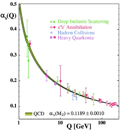
Figure 11: ${\overline{MS}}$ running coupling: compilation of experimental results from [30].

However my purpose here is not to dwell upon these calculations in any detail, but to point out that there have recently [31] been calculations of this kind in SU(4). I show the corresponding plot, borrowed from [31], in Fig. 12. The range of energies is less impressive but is still non-trivial. Extracting the $\Lambda$ parameter from the fits, and converting to the standard $\overline{MS}$ scheme, and using the results of earlier calculations for $N=2$ and $N=3$, one finds [31]

$$\frac{\Lambda_{\overline{MS}}}{\surd\sigma}=0.528(40)+\frac{0.18(36)}{N^{2}}\qquad:N\geq 3$$ (31)

Since this is a straight-line fit to just 2 points, $N=3$ and $N=4$, it will require further confirmation, but it is reassuring that it is consistent with the result in eqn(30), obtained from the quite different approach of fitting the running of the bare lattice coupling.

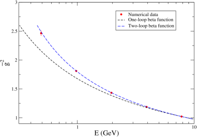
Figure 12: Continuum running coupling in SU(4) in the SF scheme from [31].

3.5 How hard are large $N$ lattice calculations?

In the pure gauge theory, we are mostly calculating products of $N\times N$ matrices, and the computational cost of that clearly increases as $\propto N^{3}$. The Monte Carlo update of the matrices proceeds by updating the SU(2) sub-groups (using standard Cabibbo-Marinari). This cost grows only as $\propto N^{2}$ if one updates all the subgroups and so is relatively unimportant. The $O(N^{3})$ increase in cost can be partially reduced if one takes advantage of the fact that one can often work on a small volume (as long as $l>1/T_{c}$) at large $N$. As an extreme example, the deconfining transition [22, 32] can be calculated with just about the same precision on $10^{3}5$ lattices in SU(8) as on $64^{3}5$ lattices in SU(3). Here the volume gain more than outweighs the $N^{3}$ loss. And for a dramatic example of this, at very large $N$, see the string tension calculation in [33].

The above has to do with how the cost in generating a single lattice field grows with $N$. However the relevant question is what is the cost of achieving a given error/signal ratio in the calculation of some physical quantity like the mass gap.

Indeed, since we calculate masses from connected correlators of traced operators, i.e. correlations between singlet fluctuations, and since we know that all such fluctuations vanish as $N\to\infty$, one might wonder whether this renders mass calculations impossible in that limit.

The answer is no: the errors on the fluctuations are themselves determined by higher order correlators, which generically vanish at the same rate in the pure gauge theory. For example consider $C(t)=\langle\phi^{\dagger}(t)\phi(0)\rangle$ where $\phi$ is a trace of some gauge field operator, and $\langle\phi\rangle=0$ so that there is only the disconnected piece to consider. Then in a numerical estimate of $C(t)$ its fluctuation squared is proportional to the higher order correlator $\langle[\phi^{\dagger}(t)\phi(0)-C(t)]^{2}\rangle$. An analysis of this using the usual large $N$ counting rules, shows that both the average value of the correlator and the fluctuation around that average disappear with the same power of $N$. That is to say, as $N\to\infty$ there are no extra hidden costs to extracting masses from correlation functions.

Figure 13: How the fluctuations on a physically relevant connected correlator, at $t=0$ ($\bullet$) and $t=a$ ($\circ$), vary with $N$.

To see what happens in practice, I show in Fig. 13 how the error to signal ratio on $C(t=0)$ and $C(t=a)$ varies as a function of $N$, when we perform the same number of Monte Carlo sweeps, on the same size lattice, and for the same lattice spacing [18]. The correlator is one used to calculate a physical quantity, so we infer that the difficulty of calculating a mass does not grow with $N$ beyond the growing difficulty of generating the lattice fields themselves.

Turning now to the inclusion of quarks fields in the fundamental representation, the most expensive part of current calculations, even for SU(6) and even in the quenched case, is the matrix times vector multiplication (e.g. in propagators) and this is $\propto N^{2}$. This may in principle be partly offset by smaller finite $V$ corrections at larger $N$.

If one now looks at connected correlators (in the quenched case) and at the higher order correlators that determine their fluctuations, one finds [19] that the latter generically vanish not at the same rate, but as $O(1/N)$ – which translates into an effective improvement of $\propto N^{2}$ in statistics. This gain of $N^{2}$ will compensate the increase in cost of multiplying matrices by vectors, so that increasing $N$ leads to no increase in cost. In practice this ideal is not achieved and the total cost of calculating a mass to a certain accuracy grows roughly as $\propto N$ [19].

Let me emphasise here that all current calculations have been performed on a small number of desktops or on a modest cluster. Large $N$ calculations are thus accessible to all of you!

4 Large $N$ Physics at high $T$

The finite $T$ physics of QCD is very topical because of the dedicated experimental programme at RHIC and the upcoming experiments at the LHC (where the ALICE detector is dedicated to this physics). The experiments have confirmed earlier lattice indications that for quite a large range of $T$ above the deconfining temperature, $T_{c}$, the plasma is strongly interacting and apparently out of reach of straightforward perturbative expansions.

At the same time, this has become a topical arena for gauge-gravity duality calculations. Of course, such (top-down) approaches are typically applicable to ${\cal{N}}=4$ SUSY, and various deformations thereof. And they are only valid in the limit of $N$ and $g^{2}$ both large. None of this looks very much like QCD or SU(3) gauge theory in the low-$T$ confining phase. However at finite $T$, the adjoint fermions in ${\cal{N}}=4$ SUSY acquire $O(T)$ Matsubara masses, from the anti-periodic fermionic boundary conditions in the Euclidean time (thermal) direction. Once SUSY is broken in this way, the adjoint scalars are no longer protected from acquiring a mass, and will also become massive. Thus the only remaining light fields are the gauge fields – which begins to look like a gauge theory at $T>T_{c}$. Moreover, since the real-world plasma appears to be strongly coupled, this begins to look like an ideal area for applying gauge-gravity duality. Of course all the AdS/CFT calculations are at large $N$ so it is important to check if for the relevant thermodynamic quantities, $N=3$ is close to $N=\infty$. This is what I want to focus upon in this section.

Euclidean lattice calculations of thermal averages are straighforward. One takes the Euclidean time torus to be of length $l_{t}=aL_{t}$, and imposes (anti)periodic boundary conditions for (fermions) bosons. The path integral is then just the partition function of the quantum field theory at a finite temperature $T=1/l_{t}$, or $aT=1/L_{t}$ in lattice units:

$$Z=\int\prod_{l}dU_{l}e^{-\beta S}=\sum_{n}e^{-\frac{E_{n}}{T}}$$ (32)

Of course we should also make the spatial tori large enough, $L_{i}\gg L_{t}$, so that we are in the thermodynamic limit, where we have a well-defined notion of temperature.

4.1 Deconfinement

What do we expect?

If the transition is first order (as indeed it is for $N\geq 3$ in $D=3+1$ and for $N\geq 4$ in $D=2+1$) it will occur at the value of $T$ at which the free energies of the confined and deconfined phases become equal, $F_{c}=F_{d}$. Now, since the number of gluons is $O(N^{2})$ we expect $F_{d}\propto N^{2}$. On the other hand we might naively expect $F_{c}\propto N^{0}$, since there are only colour singlet states in the confined phase. If so, it immediately follows that $T_{c}\to 0$ as $N\to\infty$.

From our numerical results we know that this does not in fact happen. The reason is easy to see: in the confined phase there is a $-O(N^{2})$ contribution to $F_{c}$ that comes from the vacuum energy density (the gluon condensate). So in the large $N$ limit, the value of $T_{c}$ is precisely determined by the balance between this $O(N^{2})$ vacuum contribution to $F_{c}$ and the $O(N^{2})$ piece of $F_{d}$. If the plasma had turned out to be weakly coupled, we could have easily calculated $F_{d}$ and therefore obtained a direct relationship between $T_{c}$ and the gluon condensate. That would have been very nice, but as it happens the plasma is strongly coupled, and so we have no such relation – but, on the other hand, this opens the door to AdS/CFT calculations.

In Fig. 14 I show lattice calculations of $T_{c}$ in units of the string tension for $N\in[2,8]$ in $D=3+1$. All the values shown are after extrapolation to the continuum limit [22]. If we fit with an $O(1/N^{2})$ correction we obtain

$$\frac{T_{c}}{\surd\sigma}\stackrel{{\scriptstyle N\geq 2}}{{=}}0.597(4)+\frac{0.45(3)}{N^{2}}\qquad:\quad D=3+1$$ (33)

which thus provides a prediction $\forall N$. It is perhaps surprising that this simple analytic form should fit all the way down to $N=2$ where the transition has changed from first to second order. Especially so, given that the errors for SU(2) and SU(3) are very small, about 0.5%. We also note that the coefficient of the correction is $O(1)$ in natural units.

Figure 14: Deconfining temperature in units of the string tension, for continuum SU($N$) gauge theories in $D=3+1$; with $O(1/N^{2})$ extrapolation to $N=\infty$.

It is interesting to see what happens in $D=2+1$. The corresponding results for $T_{c}$ [34] are shown in Fig. 15. Now both $N=2$ and $N=3$ are second order, but a fit with just the leading correction still works for all $N$, giving

$$\frac{T_{c}}{\surd\sigma}\stackrel{{\scriptstyle N\geq 2}}{{=}}0.903(3)+\frac{0.88(5)}{N^{2}}\qquad:\quad D=2+1$$ (34)

where again the size of the correction is modest in natural units.

Figure 15: As in Fig. 14 but for $D=2+1$.

Most but not all thermodynamic quantities associated with the deconfining transition show a modest variation with $N$ [32, 35]. A striking counterexample is provided by the interface tension, $\sigma_{cd}$, between the confining and deconfining phases. Although this calculation is difficult, one roughly finds [32].

$$\frac{\sigma_{cd}}{T^{3}_{c}}\stackrel{{\scriptstyle N\geq 3}}{{=}}0.0138(3)N^{2}-0.104(3)\qquad:\quad D=3+1$$ (35)

Here the coefficient of the subleading term is very large compared to that of the leading term. Because of this the value of $\sigma_{cd}$ is anomalously small for SU(3), and this is presumably the main reason why the phase transition appears to be very weakly first order in this case.

4.2 A strongly coupled gluon plasma?

We now want to ask whether the gluon plasma continues to be strongly coupled at large $N$. One of the measures of this is the pressure and its deviation from the Stefan-Boltzmann value. I will focus on this here because the lattice calculation is particularly simple. (I reproduce the argument given in [36].)

The pressure is the (infinitesimal) work done when the volume increases (infinitesimally). So it can be obtained from the change in the average energy as we increase the volume, using eqn(32),

$$p=T\frac{\partial}{\partial V}\log Z(T,V)=\frac{T}{V}\log Z(T,V)=-f$$ (36)

where the second equality assumes a sufficiently large and homogeneous system, and $f=F/V$ is the free energy density. To calculate the pressure at temperature $T=1/aL_{t}$ in a volume $V=a^{3}L^{3}_{s}$ with lattice cut-off $a(\beta)$, it is convenient to express $\log Z$ in the integral form:

$$p(T)=\frac{T}{V}\log Z(T,V)=\frac{1}{a^{4}(\beta)L_{s}^{3}L_{t}}\int^{\beta}_{\beta_{0}}d\beta^{\prime}\frac{\partial\log Z}{\partial\beta^{\prime}}.$$ (37)

There is in general an integration constant, but it will disappear when we regularise the pressure in a moment. This integral form is useful because it is easy to see from Eqs. (32,8) that

$$\frac{\partial\log Z}{\partial\beta}=-\langle S\rangle=N_{p}\langle u_{p}\rangle$$ (38)

where $N_{p}=6L_{t}L^{3}_{s}$ is the total number of plaquettes and $u_{p}\equiv{\rm Re}\Tr{U_{P}}/N$.

So the pressure can be obtained by simply integrating the average plaquette over $\beta$: a very simple calculation. This pressure has been defined relative to that of the unphysical ‘empty’ vacuum and will therefore be ultraviolet divergent in the continuum limit. To remove this divergence we need to define the pressure relative to that of a more physical system. We shall follow convention and subtract from $p(T)$ its value at $T=0$, calculated with the same value of the cut-off $a(\beta)$ (so that the UV divergences cancel). Thus our pressure will be defined with respect to its $T=0$ value. Doing so we obtain from eqns(38, 37)

$$a^{4}[p(T)-p(0)]=6\int^{\beta}_{\beta_{0}}d\beta^{\prime}(\langle u_{p}\rangle_{T}-\langle u_{p}\rangle_{0})$$ (39)

where $\langle u_{p}\rangle_{0}$ is calculated on some $L^{4}$ lattice which is large enough for it to be effectively at $T=0$. We replace $p(T)-p(0)\to p(T)$, where from now on it is understood that $p(T)$ is defined relative to its value at $T=0$, and we use $T=(aL_{t})^{-1}$ to rewrite eqn(39) as

$$\frac{p(T)}{T^{4}}=6L^{4}_{t}\int^{\beta}_{\beta_{0}}d\beta^{\prime}(\langle u_{p}\rangle_{T}-\langle u_{p}\rangle_{0}).$$ (40)

We remark that when our $L_{s}^{3}L_{t}$ lattice is in the confining phase, then $\langle u_{p}\rangle$ is essentially independent of $L_{t}$ and takes the same value as on a $L^{4}_{s}$ lattice. This should become exact as $N\to\infty$ but is accurate enough even for SU(3). Thus as long as we choose $\beta_{0}$ in eqn(40) such that $a(\beta_{0})L_{t}>1/T_{c}$ then the integration constant, referred to earlier, will cancel.

We calculate the pressure using eqn(40) on a volume that is large enough to be effectively infinite. Since the plasma has a mass gap (the electric and magnetic screening masses) this is easy to achieve. We then normalise it to the Stefan-Boltzmann value (in an infinite volume). It has long been known that this ratio is far below unity, even to quite high $T$, for SU(3). This is now considered to be a reflection of the strong coupling nature of the gluon plasma.

A simple strategy is to perform similar calculations at larger $N$ and see whether this ratio continues to remain far from unity or not. This was first done in [36] where it was shown that there is essentially no change in the normalised value of $p/T^{4}$ as one increases $N$ from $N=3$ to $N=8$, in the range $1\leq T/T_{c}\leq 2$. Recently [37] there has been a more accurate calculation extending over a larger range of $T/T_{c}$, and in Fig. 16 I show the relevant plot (borrowed from [37]). We see that any variation is negligible: the $N=\infty$ plasma is just as strongly coupled as the $N=3$ one.

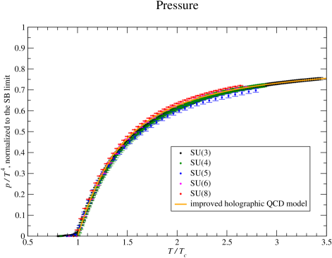
Figure 16: Normalised pressure above $T_{c}$ for various SU($N$) gauge theories [37].

This is of course good news for the applicability of AdS/CFT to real world experiments above $T_{c}$. (And you can see a comparison with one such calculation in Fig. 16.) In addition, it restricts what dynamics we might think is responsible for the strong coupling, if we make the plausible assumption that this dynamics should be common to all SU($N$) gauge theories. For example, it excludes an important role for topology (since we know that in the deconfined phase topological fluctuations vanish roughly exponentially with $N$ [35, 27]) or for any colour singlet hadrons that might survive above $T_{c}$.

5 And if I had the time …

There are many other topics on which there has has been significant progress, and which I would have liked to describe to you if there had been time. Here I will just list some of them:

$\bullet$ space-time reduction

$\bullet$ large-$N$ phase transitions

$\bullet$ topology at large $N$

$\bullet$ interlaced $\theta$-vacua

$\bullet$ chiral symmetry breaking at large $N$

$\bullet$ topology and chiral symmetry breaking

$\bullet$ strong coupling

$\bullet$ full glueball spectrum and the Pomeron

$\bullet$ $k$-string tensions in $D=2+1$ and $D=3+1$

$\bullet$ Karabali-Nair Hamiltonian approach in $D=2+1$: lattice tests

6 Flux tubes as strings

6.1 General considerations

Suppose we place a static fundamental source in our SU($N$) gauge theory at $\vec{x}=(0,y,z)$, with a conjugate source at $\vec{x}=(r,y,z)$. Suppose our space-time is a 4-torus, with the Euclidean time extent being $\tau$, and that we are in the confining phase. As usual we denote by $Z$ the partition function of the field theory on the given space-time. We also define a partition function for the system with these sources by

$$Z_{s\bar{s}}(r,\tau)=\int dA\ l^{\dagger}(x=r,y,z)l(x=0,y,z)\,\exp\{-S[A]\}$$ (41)

where $l(\vec{x})$ is the traced, path-ordered exponential of the gauge potential along a path that encircles the t-torus and is at $\vec{x}=(x,y,z)$. This is often called a Wilson line, or a Polyakov loop, and, sometimes, a thermal line. It is the phase factor that arises from the minimal coupling of the static sources to the gauge fields, $j_{\mu}A_{\mu}=j_{0}A_{0}$. In Section 7 we shall see how this translates to the lattice, but for now we shall use a continuum language.

If $r\gg 1/\surd\sigma$ there will be a flux tube between the sources which, as it evolves in time, sweeps out a sheet bounded by the periodic sources. (I am making some assumptions e.g. that the spatial torus is $\gg r$.) This sheet clearly has the topology of a cylinder. The partition function can be written as a sum over states

$$\frac{1}{Z}Z_{s\bar{s}}(r,\tau)=\sum_{n}\omega_{n}e^{-E_{n}(r)\tau}$$ (42)

where $E_{n}(r)$ is an energy level of two sources separated by $r$, and $\omega_{n}$ is its degeneracy. The states are (excited) flux tubes that begin and end on a source and which evolves around the $t$-torus. The artifice of static sources, means that the flux tube states have zero transverse as well as zero longitudinal momentum.

Now, there is another way to look at this set-up. We are in Euclidean space time so we are free to think of any of our axes as being the time direction, with its associated Hamiltonian defined on the space spanned by the other three coordinates. Taking $x$ as labelling the ‘time’, $l$ is now a Wilson line that winds around what is now a spatial torus of length $\tau$. What $Z_{s\bar{s}}(r,\tau)$ represents, in this point of view, is a correlation function whose intermediate states consist of flux tubes that wind around this same ‘spatial’ torus of length $\tau$ and propagate the distance $r$ between the two Wilson lines. The same partition function can therefore also be written as

$$\frac{1}{Z}Z_{s\bar{s}}(r,\tau)=\sum_{n,p}c_{n}(p,\tau)e^{-\tilde{E}_{n}(p,\tau)r}$$ (43)

where $\tilde{E}_{n}$ is an energy level of the (excited) flux tube that winds around a spatial torus of length $\tau$. The $\tilde{E}_{n}$ and $E_{n}$ are different functions in general because the flux tubes have have different boundary conditions. (Often, where the context removes any ambiguity, I will use $E_{n}$ in place of $\tilde{E}_{n}$, and I will be casual about distinguishing energy levels from energy eigenstates.) Here I have made explicit that the winding flux tubes have to be integrated over transverse momentum $p$ since the operators $l$ are localised at $y,z$. The $c_{n}$ are the wave-function factors for the overlap of a state $|n,p\rangle$ on the operator $l$: $c_{n}=\sum_{i}|\langle vac|l^{\dagger}|n,i,p\rangle|^{2}$, where the sum is over the degenerate eigenstates contributing to the energy level $n$. Lorentz invariance enables us to do the integral over $p$ [38, 39] but I will not pursue that explicitly here.

You may be wondering how one shows that a Polyakov loop correlator only involves winding eigenstates (even if this is heuristically plausible). I will give the argument in Section 7.1.

The above two ways of writing the Polyakov loop correlator, either as a sum over closed strings or as a sum over open strings, is a duality that has been well-known since the early ’80’s, and has been used routinely in numerical simulations. However the interesting thing for us about this open-closed string duality is the relatively recent realisation [38] that it strongly constrains the form of the effective string theory describing the dynamics of long flux tubes.

So suppose that we have an effective string theory, governed by an effective action $S_{eff}$, which reproduces the long distance physics of flux tubes. Consider the string partition function over the $r\times\tau$ cylinder considered above. We will have

$$Z_{cyl}(r,\tau)=\int_{cyl=r\times\tau}dSe^{-S_{eff}[S]}=\frac{1}{Z}Z_{s\bar{s}}(r,\tau)$$ (44)

where we integrate over all surfaces $S$ spanning the cylinder. From eqn(44) we infer that $Z_{cyl}(r,\tau)$ can be written as a sum of open or closed strings as in eqn(42) and eqn(43). These are nothing but Laplace transforms, in $r$ and $\tau$ respectively of $Z_{cyl}(r,\tau)$. So if we have a candidate string action, $S_{eff}[S]$, we can perform these Laplace transforms and extract the open and closed string spectra. Conversely, the particular form of the Laplace transforms in eqns(42,43), and in particular the way Lorentz invariance constrains the energy levels of different $p$ in eqn(43), will constrain the permitted form of $S_{eff}[S]$ and this may in turn constrain the possible form of the flux tube energy spectrum.

In the above we have specifically discussed the open-closed duality [38] associated with a cylinder. One can usefully extend [40] such a discussion to an $r\times\tau$ torus and its associated closed-closed string duality. Now we would have

$$Z_{torus}(r,\tau)=\int_{T^{2}=r\times\tau}dSe^{-S_{eff}[S]}=\sum_{n,p}\tilde{\omega}_{n}e^{-\tilde{E}_{n}(p,\tau)r}=\sum_{n,p}\tilde{\omega}_{n}e^{-\tilde{E}_{n}(p,r)\tau}$$ (45)

and a useful new constraint on $S_{eff}[S]$ [40]. It is clear that we have not exhausted all the possibilities here and that other boundary conditions may provide further useful constraints.

Some comments. (For a more detailed discussion, see [40].)

As is well-known, string theories are not well-defined outside their critical dimension. However the resulting anomalies, which show up in different ways depending on how one ‘gauge-fixes’ the diffeomorphism invariance in one’s calculation, typically die off at long distances, e.g. [41], and when one considers a long string [42]. Thus it can make sense, at least technically, to consider a string path integral over a single large surface, in an effective string theory approach outside the critical dimension [42]. This represents the world sheet swept out by a single long fluctuating string.

This effective string theory approach is therefore limited to describing the dynamics of a single long fluctuating flux tube. This is an important physical limitation. In reality, a sufficiently excited flux tube can decay into a flux tube of lower energy and a glueball, and such states inevitably appear in the sum over states in eqn(42) and eqn(43). In the string picture a glueball is a contractible closed loop of string whose length is $O(1/\surd\sigma)$ (for light glueballs). There is no guarantee that an effective string theory can consistently describe such extra small surfaces. One can partially circumvent this by only considering low-lying string states which are too light to decay:

$$E_{n}(r)-E_{0}(r)\ll m_{G}.$$ (46)

However even such states will be affected by mixing through virtual glueball emission, which corresponds to small handles on our large surface - again something that would be problematic for the string theory.

There is of course a limit in which mixings and decays do vanish, and that is the $N\to\infty$ limit. So it is consistent to use eqn(44) and eqns((42,43) for the SU($\infty$) theory. It is then plausible that as we move continuously away from that limit, to finite $N$, the corrections will be under control and small [40]. Indeed, we shall see that the low-lying flux tube spectrum has very little $N$-dependence for $N\geq 3$, and this increases our confidence in the potential applicability of the effective string theory approach to SU($N$) gauge theories in general.

Let us consider a flux tube that winds around a spatial torus of length $l$. (We shall often use $l$ in place of $r$ and $\tau$.) The excited states of this flux tube are presumably obtained from the ground state, $E_{0}(l)$, by exciting some of the modes living on the tube. If the excited mode is massive we would expect

$$E_{n}(l)=E_{0}(l)+O(\surd\sigma).$$ (47)

If the modes are massless, we would expect the extra energy to be given by their momenta which, for bosons, is quantised to be $p=k\pi/l;k=\pm 1,...$ on such a periodic flux tube. (So to obtain an excited flux tube with zero net longitudinal momentum, we will need more than one such excitation if, as is usually the case, a $k=0$ mode is not allowed.) So we expect

$$E_{n}(l)=E_{0}(l)+O\left(\frac{\pi}{l}\right).$$ (48)

So at large $l$, where $\pi/l\ll\surd\sigma$, the low-lying flux-tube spectrum is given solely by the excitation of the massless modes.

The first step is therefore to focus on an effective string action that includes just these massless modes. In general we expect modes to be massless for symmetry reasons. In the case of a flux tube there are $D-2$ obvious massless modes. These are the Goldstone modes that arise from the fact that once we have specified the location of our flux tube, we have broken spontaneously the translation invariance in the $D-2$ directions transverse to the flux tube. Of course it may be that there are other less obvious massless modes. However it clearly makes sense to start with just these Goldstone modes and to calculate from them properties of the low-lying flux tube spectrum for long flux tubes. If these agree with what we find through our direct lattice calculations of the spectrum, we can be confident that we have identified correctly all the massless modes.

To proceed one needs to fix convenient coordinates to describe the surface in the path integral. This is a ‘gauge-fixing’ of the diffeomorphism invariance, and in so doing we risk making the constraints that follow from this fundamental string symmetry less obvious. Here we follow [43, 38, 40] and do not discuss the details of the important alternative approach [42]. Suppose we are integrating over the surfaces of the cylinder discussed above. There is a minimal surface which we can parameterise by $x\in[0,r]$ and $t\in[0,\tau]$. Other surfaces are specified by a transverse displacement vector $h(x,t)$ that has two components in the $(y,z)$ directions. (This is for $D=3+1$; it has only one component for $D=2+1$.) This way of parameterising a surface is often called ‘static gauge’. We can now write the effective string action in terms of this field $h$; schematically,

$$S_{eff}[S]\longrightarrow S_{eff}[h]$$ (49)

and the integral over surfaces becomes an integral over $h(x,t)$ at each value of $(x,t)\in[0,r]\times[0,\tau]$. Since the field $h$ is an integration variable in $(0,\infty)$, we can take it to be dimensionless. Moreover, since the action cannot depend on the position of the flux tube (translation invariance), it cannot depend on $\langle h\rangle$ but only on $\partial_{\alpha}h$ where $\alpha=x,t$. That is to say, schematically,

$$S_{eff}[h]\longrightarrow S_{eff}[\partial h]$$ (50)

and we can perform a derivative expansion of $S_{eff}$ in powers of derivatives of $h$; (very) schematically

$$S_{eff}=\sigma r\tau+\int^{\tau}_{0}dt\int^{r}_{0}dx\frac{1}{2}\partial h\partial h+\sum_{n=2}c_{n}\int^{\tau}_{0}dt\int^{r}_{0}dx(\partial h)^{2n}$$ (51)

where the derivatives are with respect to $x$ and $t$ and indices are appropriately contracted. The coefficients $c_{n}$ have dimensions [length]^(2n-2) to keep the terms dimensionless. So we can expect that for the long wavelength fluctuations of a long string, such a higher order term will make a contribution of $O(1/(\sigma l^{2})^{n-1})$ and so the importance of these terms is naturally ordered by the number of derivatives. All this is entirely analogous to the familiar way chiral Lagrangians depend on their Goldstone fields.

Three comments.
$\bullet$ The approach just described is typically designed to capture the physics on energy scales smaller than a dynamical mass scale. Here that would be $O(\surd\sigma)$. Just as the applicability of chiral Lagrangians is typically bounded by the lowest resonances.
$\bullet$ For simplicity of presentation we ignore operators that are located on the boundary of the cylinder.
$\bullet$ Such an expansion is unlikely to be better than asymptotic, and so might well have corrections that are perhaps like $\exp\{-1/(\partial h)^{2}\}$ that will lead to corrections like $\exp\{-c\sigma l^{2}\}$ in the spectrum. More generally we need to be cautious about the uniformity of the various limits being taken in any applications (e.g. large $n$, $r$, $\tau$).
$\bullet$ Our chosen ‘static-gauge’ parameterisation does not work for general surfaces. To describe a string with an ‘overhang’ or any kind of ‘back-tracking’, the field $h(x,t)$ would have to multivalued, which is something the standard treatments do not allow. That is to say, we arbitrarily exclude such rough surfaces from the path integral. For a flux tube, its finite width provides a physical lower distance cutoff on such fluctuations: any overhang that is within a distance $\lesssim 1/\surd\sigma$ will in effect be a fluctuation in the intrinsic width of the flux tube i.e. a massive mode excitation. Any backtracking/overhang that is larger will increase the length by $\Delta l>1/\surd\sigma$ and hence the energy by $\Delta E\sim\sigma\Delta l>\surd\sigma$. In both cases the associated excitation energies will be much greater than the $O(1/l)$ gap to the stringy modes, once $l$ is large enough. Thus this should not be a significant issue for the long wavelength massless oscillations we have discussed above. But it needs to be addressed in any analytic treatement that wishes to be more ambitious.

6.2 The Gaussian approximation

The first non-trivial term in our effective string action is the Gaussian piece:

$$S_{eff}=\sigma r\tau+\int^{\tau}_{0}dt\int^{r}_{0}dx\frac{1}{2}\partial_{\alpha}h\partial_{\alpha}h$$ (52)

Since it has the fewest derivatives it should provide the leading correction to the linear piece of the string energy, at large $l$. (For the cylinder there is a linear piece, $\propto\tau$, that comes from the boundary of the cylinder, and represents a self-energy term for the source. We ignore that in the following.) Being Gaussian, this can be calculated exactly, and one obtains

$$Z_{cyl}(r,\tau)=e^{-\sigma r\tau}|\eta(q)|^{-(D-2)}\quad:\quad q=e^{-\pi\tau/r}$$ (53)

in terms of the Dedekind eta function

$$\eta(q)=q^{\frac{1}{24}}\prod^{\infty}_{n=1}(1-q^{n}).$$ (54)

(See [38] whose notation I will borrow.) If we expand the product in eqn(54) we have a sum of powers of $q$, which, using $q=e^{-\pi\tau/r}$, becomes a sum of exponentials in $\tau$ which is precisely of the form given in eqn(42). So matching this result with eqn(42), we obtain the prediction

$$E_{n}(r)=\sigma r+\frac{\pi}{r}\left\{n-\frac{1}{24}(D-2)\right\}$$ (55)

for the energy levels. In addition, one also obtains predictions for the degeneracies of these levels. This is the exact result, for a Gaussian $S_{eff}$, for the energy levels of strings with ends fixed to static sources. We note that the excitation energies display an $O(1/r)$ gap as expected from eqn(48).

The Dedekind eta function possesses a well-known modular invariance:

$$\eta(q)=\left(\frac{2r}{\tau}\right)^{\frac{1}{2}}\eta(\tilde{q})\qquad;\quad\tilde{q}=e^{-4\pi r/\tau}.$$ (56)

and so using eqn(54), but now for $\eta(\tilde{q})$, we can rewrite the expression for $Z_{cyl}$ in eqn(53) as a sum of exponentials in $r$ rather than in $\tau$. However this is not precisely of the form shown in eqn(43), because of the momentum integrations (which can be shown [38, 39] to lead after integration to a sum over Bessel functions rather than simple exponentials). Thus a Gaussian $S_{eff}$ does not encode the open-closed string duality exactly and cannot be considered as a candidate for an exact description of strings on a cylinder. However if we think of the Gaussian $S_{eff}$ as an approximation, possessing higher order terms that we are not considering at this stage, then at large enough $\tau$, where the Bessel functions can be expanded as exponentials to leading order, we can match with eqn(43) to obtain the closed string energies,

$$\tilde{E}_{n}(\tau)=\sigma\tau+\frac{4\pi}{\tau}\left\{n-\frac{1}{24}(D-2)\right\}+O\left(\frac{1}{\tau^{2}}\right)$$ (57)

together with an expression for the overlaps $c_{n}$ [38].

The $O(1/r)$ correction to the leading linear term in $E_{0}(r)$ in eqn(55) is the famous Luscher correction [43] for a flux tube with ends fixed on static sources. Physically it arises from the regularised sum of the zero-point energies of all the quantised oscillators on the string. It depends only on the long wavelength massless modes and so is universal: any bosonic string theory in which the only massless modes are the transverse oscillations will have precisely this leading correction. The same applies to the $O(1/\tau)$ correction to the leading linear term in $\tilde{E}_{0}(r)$ in eqn(57).

Although the above results for $E_{n}(r)$ are obtained in the Gaussian approximation to $S_{eff}[h]$, this approximation becomes exact as $r\to\infty$, and these predictions for the leading $O(1/r)$ correction are also exact and universal.

6.3 Nambu-Goto free string theory

There is only one string theory whose spectrum can be calculated in a closed form (as far as I am aware). That, not surprisingly, is a free string theory: Nambu-Goto in flat space time (see e.g. [44]),

$$Z=\int dSe^{-\kappa A[S]}$$ (58)

where we integrate over all surfaces, with the action proportional to the invariant area. This is not à priori a completely unrealistic effective string theory: after all, we recall that flux tubes at $N=\infty$ do not interact.

The energy levels of this theory were originally calculated in [45] (and were subsequently extended in various papers). Since our numerical calculations will focus on flux tubes that are closed around a spatial torus of length $l$, this is the spectrum I will present here.

Consider a string winding once around the $x$-torus. (One can readily extend this to strings winding $\omega$ times around a torus.) Perform the usual Fourier decomposition of $h(x)$. Upon quantisation the coefficients become creation operators for ‘phonons’ with momenta $\pm 2\pi k/l$ along the string and energy $2\pi k/l$ (since the modes are massless). Note that the $k=0$ mode is not included since it corresponds to a shift to a different transverse position of the whole string i.e. to another vacuum of the spontaneously broken symmetry. We call positive momenta left-moving (L) and the negative ones right-moving (R). Let $n_{L(R)}(k)$ be the number of left(right) moving phonons of momentum $2\pi k/l$. Define the total energy (and momentum) of the left(right) moving phonons as $2\pi N_{L(R)}/l$, then:

$$N_{L}=\sum_{k}\sum_{n_{L}(k)}n_{L}(k)k,\qquad N_{R}=\sum_{k}\sum_{n_{R}(k)}n_{R}(k)k.$$ (59)

If $p=2\pi q/l$ is the total longitudinal momentum of the string then, since the phonons provide that momentum, we must have

$$N_{L}-N_{R}=q.$$ (60)

We can now write down the expression for the energy levels of the Nambu-Goto string:

$$E^{2}_{N_{L},N_{R}}(q,l)=(\sigma l)^{2}+8\pi\sigma\left(\frac{N_{L}+N_{R}}{2}-\frac{D-2}{24}\right)+\left(\frac{2\pi q}{l}\right)^{2}$$ (61)

where the degeneracies corresponding to particular values of $N_{L}$ and $N_{R}$ will depend on the number of ways these can be formed from the $n_{L}$ and $n_{R}$ in eqn(59). In discussing the states, we shall often write the left and right moving phonon creation operators of (absolute) momentum $2\pi k/l$ as $a_{k}$ and $a_{-k}$ respectively, and the unexcited string ground state as $|0\rangle$.

Let us specialise to $q=0$, i.e. $N_{L}=N_{R}=n$, and make some general comments.
$\bullet$ The energy $E_{n}(l)$ can be expanded for large $l$ in inverse powers of $1/\sigma l^{2}$:

$$E_{n}(l) = \sigma l\left(1+\frac{8\pi}{\sigma l^{2}}\left(n-\frac{D-2}{24}\right)\right)^{\frac{1}{2}}$$ (62)

$$= \sigma l+\frac{4\pi}{l}\left(n-\frac{D-2}{24}\right)+O\left(\frac{1}{\sigma l^{3}}\right)$$

We note that the first correction to the linear piece is exactly as in eqn(57). Since we claimed the latter was ‘universal’, this is as it should be.
$\bullet$ The ground state energy becomes tachyonic at small $l$:

$$E^{2}_{0}(l)=(\sigma l)^{2}-\frac{\pi\sigma(D-2)}{3}<0\qquad:\quad\sigma l^{2}<\frac{\pi(D-2)}{3}.$$ (63)

One can regard it as the Hagedorn/deconfining transition in the Nambu-Goto model, where strings condense in the vacuum.
$\bullet$ The expansion of the square root expression for the energy $E_{n}$, in eqn(62), only converges for $\sigma l^{2}>8\pi n$ (ignoring the negligible $D-2$ term). So the higher the excited state, the larger is the value of $l$ before such an expansion can be employed. This tells us that the formal expansion of the action in powers of $1/l$ is not uniform in frequency – it is, in fact, only formal. One would expect this to be the case for any string action, effective or otherwise. So while the Nambu-Goto action (the invariant area of the surface) can be expanded as described above, this expansion is not uniform in energy.
$\bullet$ One can show (see Appendix C of [38]) that the Nambu-Goto model satisfies open-closed duality exactly. This is in contrast to the Gaussian string action. Thus, if this is our only constraint, the Nambu-Goto model is a viable candidate for providing a string action that simultaneously describes flux tubes attached to static sources and their dual description as winding flux tubes between Polyakov loop operators.

This has at least one important implication. When we use open-closed (cylinder) string duality to constrain terms in the effective action that are higher order in $\partial h$ (as described earlier), these constraints will be satisfied by the Nambu-Goto model. (This is also the case [46] for constraints obtained from the closed-closed duality [40] associated with surfaces on a torus.) In particular, where imposing such constraints allows us to completely fix the expansion coefficients of $E_{n}(l)$ up to some order in $1/l$, these coefficients will have to be precisely the same as those obtained by expanding the Nambu-Goto expression in eqn(62), and the corresponding expression for strings with fixed ends, to that order.

6.4 Recent theoretical progress

The seminal work in analysing flux tubes in a string description in static gauge [43] (as described above) and the later more general approach using conformal gauge [42] (not described here) led to an understanding of the universality of the leading $O(1/l)$ Luscher correction to the linear growth of the flux tube energy. Until recently there was, however, very little further analytic progress along these lines.

The situation changed in 2004 when major progress took place independently within both approaches.
1) In [38] it was shown that the open-closed duality (discussed above) could be used to provide useful constraints on the higher order terms in the expansion of the effective string action. In particular it was shown that in $D=2+1$ the next, $O(1/l^{3})$, term is also universal and the coefficient is precisely what you get by expanding the Nambu-Goto square-root expression to that order. (As we commented above, the latter has to be the case.) In $D=3+1$ the coefficent is not fixed but there is a relationship predicted between the coefficients of the two terms in the effective action that contribute at that order.
2) In [47] (and later independently in [48]) the next order was calculated within the Polchinski-Strominger framework. The same conclusion was reached as in [38] for $D=2+1$, but a stronger conclusion was obtained in $D=3+1$, where the $O(1/l^{3})$ term in the action was shown to be universal (and equal to the value in the Nambu-Goto expansion).

This year there has been further, dramatic progress. In [40] the static gauge approach was used and extended to include the constraints that arise from closed-closed (torus) duality. This enabled [40] to show that the terms up to and including $O(1/l^{5})$ are universal, and of course equal to what you get in the Nambu-Goto model. (There are some technical qualifications to this in $D=3+1$ that I am omitting.) This work demonstrated how one can extend one’s predictions for the effective string action, by finding new physical conditions that it must satisfy. One may speculate that further progress could be made by going beyond the cylinder and torus, to consider other boundary conditions for the surfaces that one is integrating over, so as to create new, more powerful constraints on $S_{eff}$.

In addition the authors of [40]) calculated the effective string action in some confining gauge theories with a gauge-gravity dual, and showed explicitly that in these cases the coefficients up to and including $O(1/l^{5})$ are indeed as predicted by their general arguments.

Finally, as I have been writing this section, some papers have appeared [49] extending the Polchinski-Strominger approach [42, 47] and also showing that the terms up to $O(1/l^{5})$ are universal. The most recent of these papers [50] makes the dramatic claim that (with certain constraints) the energy spectrum of any effective string theory is, to all orders, the same as that of Nambu-Goto.

While I have not had the time to digest the most recent papers, it is clear that this is an exciting area in which a great deal of progress is being made at this moment.

6.5 Lattice calculations - a potted history

Having spent quite a lot of time describing the analytic work, I do not have the time to do more than point briefly to some of the numerical work that has been carried out over this same period. This is particularly inappropriate because there has been a huge amount of this work, and its increasing range, sophistication and precision has provided strong motivation for the recent analytic work that I have been describing. I will just point to some work in various directions, and leave it to you to follow their references and citations to build a more detailed and balanced picture for yourselves.

In the early to mid-80’s there was already a great deal of work testing string model predictions with numerical lattice calculations, and with open-closed string duality in mind, by for example the Copenhagen group, e.g [51]. Some of the earliest numerical work that produced reliable ground state energies for closed strings and for the Luscher coefficient was in that same period [52]. The development of blocking [10] and smearing algorithms [9] in the mid-80’s finally made the accurate calculation of energies and string tensions routine.

The potential between static sources was, of course, of continued interest, but the pioneering calculations for excited string states date to the early-90’s, e.g. [53]. The interest here was both theoretical and phenomenological: the excited string states could be used in a Schrodinger equation to get predictions for the masses of hybrid mesons where some of the quantum numbers are carried by excited glue. In the 90’s there was alot of progress by the Torino group, e.g. [54], investigating numerically the match between string theory predictions for Wilson loop expectation values and what one obtains in various gauge and spin models. It is in this body of work that one first sees a prolonged and serious focus on matching the Nambu-Goto model to numerical results, a focus which became commonplace in later work. This work has continued into the 00’s with, for example, calculations in more ‘exotic’ theories [55].

In the late 90’s and early-00’s there was the first sequence of calculations [56] that was dedicated to calculating the full string spectrum (open and closed) in SU(2) and SU(3) gauge theories. In the same period, powerful new Monte Carlo techniques were developed [57] that made possible the numerical calculation of the Luscher coefficient with greater accuracy, thus confirming the earlier work that had pointed to it being in the same universality class as the simplest bosonic string model. The last decade has also seen, for the first time, reliable numerical calculations at large $N$ [1, 58, 17], in some cases for a very large $N$ indeed [33, 59]. There have simultaneously been a number of very accurate calculations of open strings, both of the ground state (i.e. the heavy quark potential) [60] and with some work on excited states [61] and work on sources in other representations than the fundamental [62]. And since the mid-00’s there has been the dedicated calculation of the spectrum of closed flux tubes, in both $D=2+1$ [23, 63, 64, 65] and $D=3+1$ [66] that I am going to devote the rest of my lectures to.

Before moving on let me say a few comparative words about calculations of Wilson loops, open strings (potentials) and closed strings (torelons). Expectations of Wilson loops are transforms of eigenspectra (although care has to be taken with the self-energies associated with the boundaries) and are an alternative way to test string models. With open strings there is a transition between short-distance perturbative physics (the Coulomb potential) and the long-distance confining physics. This is potentially of great interest (especially at large $N$) but it can introduce extra ambiguities in the extraction of the flux tube spectrum, if that is what one is primarily interested in (as we are here). The spectrum of closed flux tubes, stabilised by closing them around a spatial torus, is a particularly clean way to investigate the properties of flux tubes, and that is why we have focused on that approach in the work below.

7 The spectrum of closed flux tubes: $D=2+1$

In this Section I will discuss the energy spectrum of closed flux tubes in SU($N$) gauge theories in $2+1$ dimensions. The numerical results that I shall show are all from [23, 63, 64, 65] or from unpublished work within that collaboration.

I am not going to say much about $D=2+1$ except to remind you that the gauge coupling $g^{2}$ has dimensions of mass, so the dimensionless expansion parameter for physics on a scale $l$ will be $lg^{2}$. Thus the theory is free in the UV and strongly coupled in the IF: much like $D=3+1$ in other words. (At least in this respect.) Lattice calculations [1] have shown that the theory is linearly confining at low $T$, just like SU($N$) gauge theories in $D=3+1$. Our understanding of the dynamics of confinement, and our analytic control over the long-distance physics, is not much better in $2+1$ than in $3+1$ dimensions. (But see [67].) In many ways, the fundamental dynamical questions are similar in both dimensions and it is useful to pose them in both contexts simultaneously, as I will be doing in these lectures.

7.1 Quantum numbers and operators

Consider a confining flux tube, with the flux in the fundamental representation. Let it wind once around the $x$-torus, which we take to be of length $l$. There are a number of symmetries some of which are interesting and some of which are not.

$\bullet$ Let $p$ be the longitudinal momentum of the flux tube. By periodicity this is quantised, $p=2\pi q/l$ where $q$ is an integer. (When we are on a lattice we will express $p$ and $l$ in lattice units.) It is plausible that the ground state, with energy $E_{0}(l)$, is invariant under longitudinal translations, and so must have longitudinal momentum $q=0$. To have $q\neq 0$ a flux tube must have a deformation so that it is not invariant under longitudinal translations. That is to say, it must be excited in some non-trivial way. Thus $E^{2}(p)\neq E^{2}_{0}+p^{2}$ and the calculated value of $E(p)$ carries non-trivial dynamical information: $p$ is an interesting quantum number.

$\bullet$ By contrast, if $p_{\perp}$ is the transverse momentum then we simply expect $E^{2}(p)=E^{2}_{0}+p^{2}_{\perp}$, so $p_{\perp}$ is not, for us, an interesting quantum number.

$\bullet$ Under charge conjugation, $C$, the direction of the flux is reversed. Thus a flux tube has zero overlap onto its charge-conjugated homologue (see below) and so linear combinations of definite $C$ are trivially degenerate. (Except for SU(2) where $C$ is trivial.) Thus $C$ is not interesting and we shall consider flux tubes whose flux is in the +ve $x$ direction.

$\bullet$ Consider the 2 dimensional parity operation $(x,y)\stackrel{{\scriptstyle P}}{{\to}}(x,-y)$. It is plausible that the absolute ground state, with energy $E_{0}(l)$, is invariant under reflections, and so will have $P=+$, with the $P=-$ linear combination being null. Thus the lightest non-null $P=-$ state involves a flux-tube with a non-trivial deformation, and so $P$ is certainly an interesting quantum number. More specifically, in a string model $h(x)\stackrel{{\scriptstyle P}}{{\to}}-h(x)$ so that the its Fourier coefficients also satisfy $a_{k}\stackrel{{\scriptstyle P}}{{\to}}-a_{k}$ and hence the parity of a string excitation is simply

$$P=(-1)^{number\ of\ phonons}.$$ (64)

So the lightest $P=-$ state will have one excited phonon with $k=1$.

$\bullet$ Suppose our (x,y) torus is symmetric. Consider rotations of the flux tube by $\pi/2$, so that it winds instead around the $y$-torus, or by $\pi$ so that the flux is reversed. Both these flux tubes will have zero overlap onto the original flux tube. Thus rotations are uninteresting. (In 2 space dimensions there are, of course, no rotations around the axis of the flux tube.)

For the above reasons we choose to calculate the flux tube energy as a function of its length $l$, its longitudinal momentum $p=2\pi q/l$, and its parity $P$.

           

Figure 17: Examples of operators with non-trivial parity: $P=-,-,+,+$ starting from the left.

We now need some lattice operators whose correlators will give us the desired spectrum. The most elementary such operator is the simple Polyakov loop:

$$l_{p}(n_{y},n_{t})=\mathrm{Tr}\left\{\prod^{L}_{n_{x}=1}U_{x}(n_{x},n_{y},n_{t})\right\}$$ (65)

where $l=La$ and we take a product of the link matrices in the $x$-direction once around the $x$-torus.

That such a winding operator should couple to winding flux tubes is heuristically plausible, but we can argue a little better than that. Consider a transformation

$$U_{x}(n_{x}=L,n_{y},n_{t})\longrightarrow zU_{x}(n_{x}=L,n_{y},n_{t}),\qquad z\in Z_{N},\,\,\forall n_{x},n_{y}$$ (66)

where all links in the $x$-direction at, say, the boundary $n_{x}=L$ are multiplied by an element of the centre. This does not affect the value of any plaquette, since a $z$ will always be accompanied by a $z^{\star}$ from the conjugate link at the opposite side of the plaquette, which gives unity, and so the action is not changed. And neither is the invariant Haar group measure. Thus the weighting of this transformed field is identical to that of the original field. Moreover, by a similar argument to that for the plaquette, the product of link matrices around any contractible closed loop $l_{C}$ is invariant, since the number of $z$ and $z^{\star}$ will be the same. However a non-contractible closed loop like the Polyakov loop is not invariant: clearly $l_{p}\to zl_{p}$. We therefore see that

$$\langle l^{\dagger}_{p}l_{C}\rangle=z\langle l^{\dagger}_{p}l_{C}\rangle,\ \ \forall z\in Z_{N}\quad\Longrightarrow\quad\langle l^{\dagger}_{p}l_{C}\rangle=0.$$ (67)

(This assumes that the center symmetry is not spontaneously broken.) Eqn(67) is true for any winding loop $l_{p}$ and any closed contractible loop $l_{C}$. So the corresponding states are completely orthogonal. The contractible loops clearly generate localised states like glueballs, while the winding loops generate non-local winding states which include winding flux tubes. Note that a similar argument to that in eqn(67) tells us that $l_{p}$ and its charge conjugation, $l^{\dagger}_{p}$, are orthogonal, except in SU(2). In the continuum the field transformation in eqn(66) arises when we note that periodicity for adjoint fields implies periodicity up to a gauge transformation that is an element of the center.

The operator in eqn(65) is localised in $n_{y}$ and so has $p_{\perp}\neq 0$. If we sum over $n_{y}$, to get $l_{p}(n_{t})=\sum_{n_{y}}l_{p}(n_{y},n_{t})$ we get an operator with $p_{\perp}=0$, and from now on we assume this has been done. This operator is manifestly invariant under longitudinal translations as well, so $p=0$. It is also invariant under parity $P$. So to have $p\neq 0$ or $P\neq+$ we must introduce a deformation in the operator in eqn(65). Some examples of $P=-$ operators are shown in Fig.17. By translating such an operator by $\Delta x$ in the $x$ direction, multiplying it by the phase factor $\exp\{i2\pi q\Delta x/L\}$, and then adding all such translations, one obtains an operator with longitudinal momentum $p=2\pi q/L$. Doing so for the operator in eqn(65) would have yielded a null operator for $p\neq 0$, but for the operators in Fig.17, that will not in general be the case.

In practice, to obtain good overlaps onto any states at all, one needs to smear [9] and block [10] the ‘link matrices’ that appear in operators such as those in Fig.17. And one also needs many operators in addition to those shown here in order to have adequate overlaps onto a good number of excited states. So, as described in more detail in [63], we typically have 150-200 operators in each of our $D=2+1$ calculations.

7.2 Ground state energy

In Fig.18 I display how the energy, $E_{0}$, of the lightest flux tube in the $q=0,\,P=+$ sector of states, varies as a function of its length $l$. This is a calculation in SU(5) and at a value of the bare inverse coupling, $\beta=80$, which corresponds to a lattice spacing in physical units of $a\simeq 0.130/\surd\sigma$. (Of course the latter is something we only know after our calculation of the string tension, $a^{2}\sigma$.) This is a small value of $a$ at which $O(a^{2})$ lattice spacing corrections are known to be negligible [1, 23]. It therefore makes sense to present the values of $E_{0}$ and $l$ in physical units, as we have done in Fig.18, using the value of $a\surd\sigma$ we obtain by fitting the $L$-dependence of $aE_{0}(L)$.

Figure 18: Ground state flux tube energy in SU(5) for lattice spacing $a\surd\sigma\simeq 0.130$. Shown are fits with a Luscher correction (dashed line) and with Nambu-Goto (solid line). The linear piece of such a fit, $\sigma l$, is also shown (dots) for orientation.

Also shown in Fig.18 are the best fits with either a simple Luscher correction, $E_{0}(l)=\sigma l-\pi/6l$, or with the full Nambu-Goto result, $E_{0}(l)=\sigma l(1-\pi/3\sigma l^{2})^{1/2}$. Fitting the lattice values of $aE_{0}(L)$ as a function of $L=l/a$ gives us a value for the string tension $a^{2}\sigma$ which we then use to produce the rescaled coordinates plotted in Fig.18. We see that although the Luscher correction captures much of the deviation from linearity at small $l$, Nambu-Goto clearly works even better. I also show the linear piece of the fit, so that you can see the deviation from linearity more explicitly.

As remarked earlier, in the context of the glueball calculation in Section 2.2, the numerical calculation gets less reliable as the energy becomes large – and here that happens as $l$ becomes large. That limits how far we can go in $l$. To see what this means in practice, recall that we are looking for an exponential decay of our correlation function at large enough $t$: $C(t=an_{t})\propto e^{-aEn_{t}}$. One way to see how well this is being determined is to fit neighbouring values of $t=an_{t}$ with a simple exponential,

$$\frac{C(n_{t})}{C(n_{t}-1)}=\exp\{-aE_{eff}(n_{t})n_{t}\}.$$ (68)

If $aE_{eff}(n_{t})$ is independent of $n_{t}$ within errors for $n_{t}\geq n_{0}$, then we can fit the data with a single exponential for $n_{t}\geq n_{0}$. Clearly, the smaller the errors on $C(n_{t}\geq n_{0})$ the more reliable will be the estimate of the energy.

Figure 19: Effective energies, as in eqn(68), which lead to the energies in Fig. 18.

In Fig.19 I plot the values of a $aE_{eff}(n_{t};l)$ corresponding to the various values of $l$ in Fig.18. At the smallest values of $n_{t}$ the errors are invisible on this plot, but it is clear that we have precise control of the asymptotic exponential decay for all our values of $l$. It is also clear, however, that the range of $n_{t}\geq n_{0}$ where $aE_{eff}(n_{t};l)$ is determined with useful accuracy shrinks rapidly as $l\,\uparrow$ and that if we were to attempt a calculation at significantly larger $l$ we would soon lose control of the asymptotic exponential decay.

Let us now turn to a more precise analysis of how well the fits shown in Fig.18 actually work. There are many ways to do this, and here we do the following, in analogy with the effective energy plots just shown. We define effective coefficients (and string tensions) by

$$E_{0}(l)=\sigma_{eff}l-c_{eff}\frac{\pi(D-2)}{6l}$$ (69)

and

$$E_{0}(l)=\sigma_{eff}l\left(1-c_{eff}\frac{\pi(D-2)}{3\sigma_{eff}l^{2}}\right)^{\frac{1}{2}}$$ (70)

for the two kind of fits. We determine $a^{2}\sigma_{eff}$ and $c_{eff}$ for each pair of values $l=l_{i},l_{i+1}$ where $l_{i}\leq l_{i+1}\,\forall i$. Plotting the result in Fig.20 - the horizontal ‘error bars’ indicate the distance between the values of $l_{i}\surd\sigma$ and $l_{i+1}\surd\sigma$ - we observe that we appear to have

$$c_{eff}\stackrel{{\scriptstyle l\to\infty}}{{\longrightarrow}}1$$ (71)

in both cases. That is to say, the central charge corresponds to a bosonic string theory where the only massless modes on the flux tube are the transverse oscillations.

Figure 20: SU(5) effective central charge: from the Luscher ($\bullet$) and Nambu-Goto ($\circ$) fits in eqn(69) and eqn(70) respectively.

You may be disturbed by the ‘peak’ in $c_{eff}$ around $l\surd\sigma=3$. This is a nice example of the kind of statistical fluctuation (here $\sim 2.5$ standard deviations) which is large enough to cause some hesitation, while being small enough to arise quite regularly in numerical calculations. To check that it is indeed a statistical fluctuation, I show in Fig.21 a similar calculation, but this time in SU(4) and with greater statistical accuracy. There are other examples that I could show as well.

Figure 21: As in Fig. 20 but for SU(4).

Since the Luscher correction is only the leading correction in an expansion in powers of $1/\sigma l^{2}$, it is entirely expected that $c_{eff}(l)$ should deviate significantly from unity as $l$ decreases. What is much more of a surprise is that for the Nambu-Goto fit, $c_{eff}\simeq 1$ for all values of $l$. That is to say, the deviations from Nambu-Goto are very small at all our values of $l$, even down to $l\surd\sigma\sim 1.5$ where the flux tube is about as wide as it is long and where it no longer ‘looks’ anything like an ideal thin string.

One might imagine that any such free string-like behaviour will arise only at large $N$, if it is to arise anywhere. It is therefore interesting to go to the smallest possible $N$ and see what happens there. So in Fig.22 I show the corresponding plot for SU(2). (These calculations are fast and it is easy to achieve very high statistical accuracy.) We observe a very similar pattern to what we have seen at larger $N$. It appears that the free bosonic string theory provides a very good approximation for all $N$.

Figure 22: As in Fig. 20 but for SU(2).

Now, the Nambu-Goto expression for $E_{0}(l)$ becomes tachyonic for $l\surd\sigma<\pi/3$, as we see from eqn(61). Given that we find such good agreement with Nambu-Goto, one might ask what happens as we approach this stringy ‘Hagedorn’ transition. For $N>3$ the critical deconfining length $l_{c}\surd\sigma>\pi/3$, so we no longer have a flux tube when $l$ is reduced to $\pi/3$ and the question cannot be addressed. However for SU(2) we have a second order phase transition at $l_{c}\surd\sigma\sim 0.9$. What we find there, as shown in Fig.23, is what one would expect: as we approach $l_{c}$ the energy dependence is governed by the critical exponents appropriate to the universality class of the transition (the $D=2$ Ising model) and so vanishes linearly in $(l-l_{c})$. As $l$ increases this linear behaviour matches smoothly onto the square root behaviour of the Nambu-Goto prediction. As we see from Fig. 23 this happens before the turn-over to the would-be stringy transition at $l\surd\sigma=\pi/3$.

Figure 23: Ground state energy of closed flux tube in SU(2) when the length $l$ approaches the deconfining transition.

7.3 Excited state energies

In Nambu-Goto, the deviation of the ground state energy, $E_{0}(l)$, from $\sigma l$ is, to lowest order in $1/l^{2}$, simply the (regularised) sum of the zero point energies arising from the quantisation of all the oscillation modes of all possible wavelengths, $\lambda_{n}=l/n$. The fact that the flux tube is well-described by this at small $l$ is surprising because one would not expect that the excitations of a short fat flux tube are the same as those of a thin string. Clearly the next step is to calculate explictly the low-lying energy spectrum and see how it varies with $l$.

In Fig. 24 I show the low-lying spectrum we obtain in SU(3) at a lattice spacing $a\surd\sigma\simeq 0.174$ and for zero longitudinal momentum, $q=0$. The ground state is well fitted by Nambu-Goto as shown. This fit determines $a^{2}\sigma$ and so the predictions shown for the excited states are completely parameter-free. We find that the first excited state of the flux tube has positive parity, $P=+$, just as in the Nambu-Goto model. Moreover, as one can see from Fig. 24, it agrees well with the predicted Nambu-Goto energy, corresponding to $N_{L}=N_{R}=1$ in eqn(61), for $l\surd\sigma\geq 2$. At this value of $l$ the flux tube is almost as wide as it is long, so it is quite remarkable that the excitation energy should be so close to what one obtains from a pair of left and right moving phonons, of the longest possible wavelengths, on an ideal string.

The next four states become degenerate for larger $l$ and are already nearly so for $l\surd\sigma\simeq 3$. We find that two have $P=+$ and two have $P=-$. This degeneracy pattern is precisely as predicted by the Nambu-Goto model, where the states are $a_{1}a_{1}a_{-1}a_{-1}|0\rangle,\,a_{2}a_{-2}|0\rangle,\,a_{2}a_{-1}a_{-1}|0\rangle,\,a_{1}a_{1}a_{-2}|0\rangle$ in the notation of Section 6.3. Moreover we see that the average energy of these four states is very close to the Nambu-Goto prediction, even at quite small $l$.

Figure 24: Low-lying spectrum of $p=0$ flux tubes in SU(3), with $P=+$ ($\times$) and $P=-$ ($\circ$) states. Lines are Nambu-Goto predictions.

Of course, all this is at a particular finite lattice spacing. To see whether these results survive the continuum limit, we repeat the calculations at a lattice spacing $a\surd\sigma\simeq 0.087$, which is smaller by about a factor of two. (We also increase all our lattice sizes, in lattice units, by a factor of 2 so that the volume is the same in physical units.) In Fig. 25 I compare the energies obtained with the coarser and finer lattice spacings. There is no visible variation, and we can confidently assume that our results also hold in the continuum limit of SU(3).

Figure 25: Spectrum from Fig. 24, $\times$, compared to spectrum for $a\to a/2$, $\bullet$.

It is clearly interesting to see what happens as we go to larger $N$ since that is the limit in which the effective string description has the most compelling motivation. In Fig.26 I compare what one obtains in SU(6) and SU(3) at a (nearly) common value of $a\surd\sigma\sim 0.17$. There is clearly very little $N$-dependence. So what we are finding is also representative of SU($\infty$) in the continuum limit.

Figure 26: Spectrum from Fig. 24, $\times$, compared to SU(6) spectrum, $\bullet$, at the same $a$.

We now turn to flux tubes that have a non-zero longitudinal momentum. As we remarked earlier, a flux tube with $q\neq 0$ must possess a deformation if it is not to be null state, so this will provide us with further information about the excitation spectrum. Moreover, since the energy of the ground state in any sector with given quantum numbers is usually the one that has the smallest systematic errors in our variational calculation, this will enable us to obtain the corresponding flux tube excitation energies with no ambiguity.

In Figs. 27 and  28 I show the results for the lowest non-zero momenta, $q=1$ and $q=2$. We see that the ground states in each case fall very precisely onto the parameter-free Nambu-Goto prediction and that they have the same quantum numbers as in the Nambu-Goto spectrum, i.e. $P=-$ with $q=1$ (corresponding to $a_{1}|0\rangle$) and a pair of degenerate $P=+$ and $P=-$ states with $q=2$ (corresponding to $a_{1}a_{1}|0\rangle$ and $a_{2}|0\rangle$). We also note that the energies of the excited states are, in each case, very close to the Nambu-Goto prediction, although their large energies (especially for $q=2$) means that the systematic errors are likely to be significant.

Figure 27: Spectrum of closed flux tubes with $p=2\pi/l$ in SU(3). Nambu-Goto predictions shown, including $p=0$ ground state from which we extract $a\surd\sigma$.

Figure 28: As in Fig. 27 but for $p=4\pi/l$.

7.4 Comparison with theory

The fact that the physical flux tube has an excitation spectrum so similar to that of a free string theory is striking and, especially at small $l$, counter-intuitive. However, as we described in Section 6.4, recent analytic studies have shown that the effective string action, when expanded in powers of $1/l$, is the same as the Nambu-Goto action up to $O(1/l^{5})$. It is natural to ask whether what we have seen is no more than a reflection of these results.

To answer this question we show again the $q=0$ SU(3) spectrum in Fig.29, but this time accompanied by the theoretical prediction to $O(1/l)$ [43, 42] that one obtains from the leading Gaussian approximation (the ‘Luscher correction’), the one to $O(1/l^{3})$ obtained by Luscher and Weisz, and by Drummond in 2004 [38, 47, 48] and finally the one to $O(1/l^{5})$ obtained this year by Aharony and collaborators [40]. (To decrypt the figure, use the rule that the curves that are higher order in $1/l$ are closer to the Nambu-Goto curves at larger $l$.)

Figure 29: Spectrum as in Fig 24 with full NG predictions (solid) and the derivative expansion (dashed) to $O(1/l)$, $O(1/l^{3})$, and $O(1/l^{5})$.

We see that for the ground state these theoretical predictions do indeed approach the numerically determined energy as we include terms of higher order in $1/l$. However this is not the case for the excited states, where there is no tendency to approach the data – at least for $l\surd\sigma<4$ for the first excited level and $l\surd\sigma<6$ for the second excited level. Indeed the oscillating behaviour of the fits as we add extra terms is instantly reminiscent of the behaviour of a series outside its radius of convergence. That this is indeed what must be happening is clear from the radius of convergence of the series expansion of the Nambu-Goto expansion:

$$E_{n}(l) = \sigma l\left(1+\frac{8\pi}{\sigma l^{2}}\left(n-\frac{D-2}{24}\right)\right)^{\frac{1}{2}}$$ (72)

$$\stackrel{{\scriptstyle n\geq 1}}{{\simeq}} \sigma l\left(1+\frac{8\pi}{\sigma l^{2}}n\right)^{\frac{1}{2}}$$

$$= \sigma l\sum_{i}c_{i}\left(\frac{8\pi n}{\sigma l^{2}}\right)^{i}\qquad\quad:\qquad\quad l\surd{\sigma}\gtrsim\sqrt{8\pi n}$$

Thus the fact that we find near-NG behaviour for $E_{n}(l)$ for $l\surd{\sigma}<\sqrt{8\pi n}$ is something that does not follow from the recent analytic developments. The latter address the $l\to\infty$ limit where $E_{n}(l)-E_{0}(l)\ll\surd\sigma$. By contrast, we find that the close agreement persists down to values of $l$ where, as we see from Fig.29, we have $E_{n}(l)-E_{0}(l)>\surd\sigma$. Thus the analytic and numerical results are largely complementary, although the fact that they both point towards the relevance of Nambu-Goto is surely no co-incidence.

7.5 Where are the massive modes?

The confining flux tube has a finite width $\sim 1/\surd\sigma$. This implies that the full description of the flux tube requires massive degrees of freedom in addition to the massless transverse oscillations encoded in the free bosonic string theory. These should make their presence felt in the observed excitation spectrum. For example, the excitations of such massive modes should lead to extra excited states with an energy gap $\Delta E\sim O(\surd\sigma)$. (At least this should be so in the simplest case of weak coupling between the different modes.)

This is a quite general expectation, whether one starts from a semi-classical intuition where one thinks of the confining flux tube as some kind of dual non-Abelian Nielsen-Olesen vortex, or whether one relies on a gauge-gravity duality intuition, where the massive modes arise from the highly non-trivial metric in the vicinity of the horizon where the string, hanging deep into the $AdS_{5}$ space, acquires its linear energy.

What is the scale of these massive modes? Obviously $O(\surd\sigma)$, but can we be more precise? Presumably this same scale appears in the spectrum of glueballs – either in the mass of the lightest glueball, or in the typical excitation energy of the lightest glueballs. Extracting the values of these from [1] we can make a plausible estimate

$$\Delta E=E-E_{0}\simeq 2\surd\sigma-4\surd\sigma.$$ (73)

Returning to the spectrum shown in Fig. 24 we find no sign of such an extra state at the smaller and intermediate values of $l$ where we have confidence in our identification of all the states with $E\lesssim 8\surd\sigma$ as being string-like. This raises two possibilities:
$\bullet$ the excitation energy of the massive modes is much larger than expected so that they effectively play no role in the spectrum at any value of $l$;
$\bullet$ our basis of lattice operators, although apparently large, has in fact a small overlap onto these massive excitations so that they do not appear in the numerically determined spectrum.
Both of these possibilities would have interesting consequences. The first would imply that we might well be able to describe most of the physics of the gauge theory within a simple bosonic string model, with other modes being so massive as to be largely decoupled. The second would suggest that there is very little mixing between these massive modes and the stringy modes, since we know that our operator basis has a good overlap onto all the light stringy modes. This again should lead to a simplification in the dynamical description of the theory. My suspicion is that the second possibility is the correct one and that with a suitably extended basis of operators we will find some massive excitations with the expected energy gap shown in eqn(73).

The above discussion suggests that it would be useful to look at other kinds of flux tubes where we know that there exist extra massive modes. This leads us smoothly onto the subject of $k$-strings.

7.6 $k$-strings

So far we have considered confining flux tubes carrying flux in the fundamental representation i.e. the kind of flux tube that forms between distant sources that are in the fundamental representation. One can also choose to consider sources in higher representations of SU($N$), and the corresponding confining tubes carrying this flux. There are however gluons in the vacuum and they can screen the sources down to other representations. This means that a flux tube will be unstable if it can be screened by gluons to a flux tube with a smaller string tension. For example the adjoint flux tube can become a state with no flux tube. (Each adjoint source being totally screened by an adjoint gluon.) As $N\to\infty$ any given unstable flux tube will become stable, and even in SU(3) it appears to make sense to discuss the qualitative properties of such flux tubes [19]. However, since what we want to obtain are quite precise calculations of energy eigenstates, an unstable flux tube, with a finite energy width, is clearly not ideal.

Fortunately some of these flux tubes are absolutely stable at larger but finite $N$. A simple way to see this is to recall that because gluons are adjoint, they do not feel the centre $Z_{N}$. So if we have a source that transforms non-trivially under the centre as

$$\psi\longrightarrow z^{k}\psi\qquad:\quad z\in Z_{N}$$ (74)

this transformation cannot change under screening. So we can categorise such sources by the value of $k$ in eqn(74). When such a source and its conjugate are far apart, the flux tube between them is often referred to, generically, as a $k$-string. If the distance is large enough it will be energetically favourable to screen the sources with gluons so that the resulting flux tube is the one with the smallest string tension in the sector of given $k$: call it $\sigma_{k}$. This flux tube is completely stable and when we speak of a $k$-string this is what we are usually referring to. (Which usage is being employed, the generic or the specific, will usually be clear from the context.) We note that $\sigma_{k=1}=\sigma_{f}=\sigma$ is just the fundamental string tension. The different values of $k$ for a given SU($N$) group are constrained by

$$z^{N}=1\qquad z^{k}=z^{N-k}\qquad:\quad z\in Z_{N}$$ (75)

which immediately implies that the non trivial values of $k$ are $k=1,2,...,[N/2]$. Thus we have to go to at least SU(4) to find a new stable flux tube of this kind.

We can think of a local source for a generic $k$ string as a localised collection of $k$ fundamental sources (heavy ‘quarks’) with any number of gluons. So the simplest example of a $k$-string is simply $k$ separate fundamental flux tubes between the $k$ fundamental sources and their conjugates. Since one finds [58, 64] that $\sigma_{k}<k\sigma$, we can think of the ground-state $k$-string as a bound state of the $k$ fundamental flux tubes.

As $N\to\infty$ we have $\sigma_{k}\to k\sigma$ and so the binding energy vanishes. Associated with the binding there will presumably be some massive excitation of the string. For example, if one imagines that the $k=2$ binding is due to the exchange of scalar glueballs between the two fundamental flux tubes, then these would provide the scale for the massive excitation. Note that even though the binding energy $\to$ $0$ as $N\to\infty$ this does not mean that the mass scale also vanishes; the loss of binding may simply be because the relevant coupling vanishes in this limit (as would be the case for our glueball exchange example). Nonetheless the fact that a $k$-string does not survive at $N=\infty$ does weaken the theoretical argument for a clean effective string theory description of the kind discussed earlier in these lectures. So, one way or another, $k>1$ flux tubes promise to provide an interesting contrast to the fundamental $k=1$ flux tubes that we have studied so far, and that is our main motivation in this Section.

Figure 30: Ground state energy of the $k=2$ flux tube, $E_{0}(l)$, normalised by its linear piece, plotted versus $l$. For SU(4) at $\beta=32$. Fits with the Luscher correction (dashed) and with full Nambu-Goto (solid) are shown.

So let us begin with the specific case of SU(4) which is the smallest group with stable $k=2$ flux tubes. It is known [58, 65] that $\sigma_{k=2}\simeq 1.35\sigma_{f}$ which implies that the two fundamental flux tubes are quite strongly bound. Associated with this binding must be some massive excitation, and we would hope to see its presence clearly encoded in the spectrum of $k=2$ flux tubes that wind around a spatial torus.

In Fig. 30 I plot the value of the ground state energy, $E_{0}(l)$, divided by its asymptotic linear component, $l\sigma_{k}$, versus the length in units of $\surd\sigma_{k}$. (For purposes of comparison with earlier figures, note that $\surd\sigma_{k=2}\simeq 1.16\surd\sigma$.) I also show a fit with a Luscher correction and a fit with Nambu-Goto. While both of these fits clearly capture a large part of the deviation from linearity, and the latter does somewhat better than the former, the Nambu-Goto fit now has significant corrections, in contrast to the case of a $k=1$ flux tube.

Figure 31: The effective central charge for $k=2$ ($\bullet$) and $k=1$ ($\circ$) flux tubes.

An alternative way to see this is to do a fit with an effective central charge, using eqn(70). We plot the result in Fig 31 together with the results obtained for a fundamental flux tube for the same lattice. We see that, while the corrections are very much larger for $k=2$ than for $k=1$, we still appear to have $c_{eff}(l)\to 1$ as $l\to\infty$, i.e. the $k=2$ flux tube also appears to belong to the universality class of the simple bosonic string theory.

Figure 32: Spectrum of lightest $k=2$ flux tubes with momenta $q=0,1,2$, in SU(4).

We now turn to the lightest states with $q\neq 0$. Our results for these are shown in Fig. 32 and are obtained in SU(4) at $\beta=50$ (so at a lattice spacing that is about 2/3 of the one considered above). For comparison we also show the $q=0$ ground state which serves to fix the value of $a^{2}\sigma_{k}$ for the $q\neq 0$ Nambu-Goto predictions. (Note we use a different normalisation than in Fig. 30, both for $E$ and for $l$.) In Nambu-Goto the $q=1$ state has one phonon and so has $P=-$, while for the $q=2$ level there are two degenerate possibilities: two phonons each with unit momentum ($P=+$) and one phonon with two units of momentum ($P=-$). We note that these are precisely the quantum numbers of the states we find, whose energies are displayed in Fig. 32. We also note that the observed energies are very close to the Nambu-Goto predictions for all values of $l$ – just as we saw for the fundamental flux tube in Figs. 27, 28.

Figure 33: The $q=1,2$ excitation energies, $\Delta E$ in eqn(76), plotted versus $l$.

Of course some of the extra energy of the $q\neq 0$ states comes from the $p^{2}$ contribution to $E^{2}(p)$ and that is not peculiar to the Nambu-Goto model. So to better expose the level of (dis)agreement with the model in eqn(61), we form the combination

$$\Delta E=\frac{1}{\pi\sigma_{k}}\left(E^{2}_{n}(l)-E^{2}_{0}(l)-\left(\frac{2\pi q}{l}\right)^{2}\right)\stackrel{{\scriptstyle NG}}{{=}}4\left(N_{L}+N_{R}\right)$$ (76)

and plot the results in Fig. 33. We see quite striking evidence for the remarkably early onset, in $l$, of agreement with this simple free string model.

Figure 34: The low-lying spectrum of closed $k=2$ flux tubes with $q=0$ and $P=+$, in SU(4).

We turn now to the first few excited $k=2$ states in the $q=0$ and $P=+$ sector, which is the analogue of the $P=+$ sector of the $k=1$ plot in Fig. 24. We plot the resulting energies in Fig. 34. We simultaneously show the predictions of the Nambu-Goto model with, as usual, the ground state fit providing the value of $a^{2}\sigma_{k}$. The contrast with Fig. 24 is quite striking. Here we have large deviations from the free string predictions, even for our longest flux tubes. In particular, we observe that the first excited state is roughly consistent with our expectation for a massive mode excitation of the flux tube, as in eqn(47). However it is also consistent with being a stringy excitation, with large corrections, which is approaching the Nambu-Goto prediction at very large $l$. One way to resolve this ambiguity is to compare the wave-function of this first excited $k=2$ excitation with that of the first excited $k=1$ excitation, since we are confident that the latter is a massless stringy mode. This was done in [65] where we showed that the wave-functions are in fact nearly identical. This makes it very likely that what we are seeing here is not the excitation of some quite different massive mode, but a conventional massless mode, albeit with large corrections to the free string result.

Figure 35: Spectrum of lightest $k=2$ flux tubes, with momenta $q=0,1,2$, in the totally symmetric representation, for SU(4).

We now briefly turn to the question of flux tubes that carry flux in different representations of SU($N$) for a given $k$. Our basis of $k=2$ operators contains two representations, the totally anti-symmetric, $k=2A$, and the totally symmetric, $k=2S$. (If we had had the foresight to use a larger basis, we would have been able to discuss other representations!) When we perform the variational calculation in this basis we find that the low-lying ground and excited states fall either into the $k=2A$ or the $k=2S$ sectors with very little mixing between the two sectors [64, 65]. In particular the lightest states with $q=0,1,2$ are $k=2A$. The energies of the corresponding $k=2S$ states are displayed in Fig. 35. These states are much heavier and consequently our calculations suffer from much greater systematic (and statistical) errors. Nonetheless it is clear that these states are also well-described by the Nambu-Goto model, albeit with a considerably larger string tension, $\sigma_{2S}$. (Aside: the $k=2S$ $q=0$ ground state would have been lighter, for some $l$, than some of the excited states shown in Fig. 34, but to avoid a messy plot I did not include it therein.) I do not show the $q=0$ excited states of $k=2S$ flux tubes: these have very large deviations from the Nambu-Goto predictions [65].

While our above foray into non-fundamental flux tubes has not uncovered any unambiguous signal for the excitation of massive modes, we have seen that at least some excitations of $k=2$ flux tubes have much larger deviations from the Nambu-Goto predictions than the $k=1$ fundamental flux tube. However the overall picture is still one of a surprising level of agreement with the free string theory, down to quite small $l$. When we consider flux in higher representations the deviations become even larger. But what appears to be the case is that such unstable ‘resonance’-like flux tubes can be labelled by the flux representation, to a good approximation, as can the corresponding tower of string-like excitations.

8 The spectrum of closed flux tubes: $D=3+1$

We are, of course, ultimately more interested in $D=3+1$ than in $D=2+1$. So what do we find if we study the closed flux tube spectrum in that case?

One difference is that one loses confinement on a slightly longer length scale: $l_{c}\surd\sigma=\surd\sigma/T_{c}\sim 1.6$ from eqn(33). The large-$l$ theoretical analysis in Section 6 goes through, with some qualifications that I will not dwell upon. And there are more quantum numbers, which is where I shall start.

The numerical results are all taken from [66]. We have performed calculations in SU(3) at two values of $a$. This enables us to confirm that what we are seeing is, to a very good approximation, the physics of the continuum theory. We also perform a calculation of the ground state in SU(6) and of the excited state spectrum in SU(5) (at the coarser lattice spacing) which allows us to confirm that there is very little $N$ dependence. We will not dwell on these points any further in the following brief overview of our current, still incomplete results and analysis.

8.1 Quantum numbers and operators

There are now two transverse directions, and so we have rotations and corresponding angular momenta around the ‘symmetry axis’ of the flux tube. The massless ‘phonons’ living on the string now carry not only momentum and energy but also unit angular momentum, with positive or negative helicity.

The quantum numbers of the flux tube can be conveniently encoded as follows.
$\bullet$ There is the length $l$ of the $x$-torus around which the flux tube winds.
$\bullet$ There is also the number of times, $w$, that the flux tube winds around this torus, but we shall only consider $w=1$ from now on.
$\bullet$ Then there is the momentum along the flux tube, $p=2\pi q/l$. (Transverse momentum is not interesting, for the same reason as in $D=2+1$.)
$\bullet$ There is the projection of angular momentum onto the symmetry axis of the flux tube, $J=0,\pm 1,...$.
$\bullet$ There is also a transverse parity, $P_{\rho}$, in the plane that is transverse to the axis, and which is analogous to the $D=2+1$ parity. Under this parity $J\to-J$. Since we choose to use this parity to label our states, we must use $|J|$ rather than $J$ as the spin label, and so when we refer to $J$, it is to be usually understood as $|J|$ from now on.
$\bullet$ For $p=0$ there is a reflection symmetry $x\to-x$ which defines a corresponding parity we call $P_{r}$; it reverses the momenta of the individual phonons.

To have a chance of a good overlap onto the ground state and some excited states for each of these quantum numbers, we need a very large basis of operators. If we imagine taking the $O(200)$ deformations we used in $D=2+1$ and using them independently in the two transverse directions, we have $\sim 40000$ operators which is much too large in practice. So instead we choose only $\sim 700$ operators.

In practice we find that our overlaps for the excited states are not nearly as good as they were in $D=2+1$, and our calculations have, inevitably, larger statistical and systematic errors. Moreover, for some quantum numbers the ground states themselves appear to have too large a mass for us to be able to extract an energy with any confidence. However even though the spectrum we obtain is incomplete, it possesses, as we shall see, some striking regularities.

8.2 Ground state energy

Our first calculation is in SU(3) at $\beta=6.0625$, which corresponds to a lattice spacing of $a\surd\sigma\simeq 0.195$. We focus on the absolute gound state, with no phonon excitations, and with quantum numbers $p=0,J=0,P_{r}=+,P_{\rho}=+$.

Figure 36: Effective central charge: from Luscher ($\bullet$) and Nambu-Goto ($\circ$) using eqns(69,70).

We perform calculations for several values of $l$, starting close to the critical value $l_{c}\surd\sigma\sim 1.55$. We then extract an effective central charge, $c_{eff}(l)$ using eqns(69,70). The resulting plot, in Fig. 36, can be compared to the similar plot for $D=2+1$ in, say, Fig. 21. At first sight they look very similar. Just as in $D=2+1$, we clearly have $c_{eff}\to 1$ as $l\to\infty$. So here too the effective string theory is in the universality class of the bosonic string theory where the only massless modes are the goldstone modes associated with the spontaneous breaking of transverse translation symmetry. Moreover we find $c_{eff}\simeq 1\,\,\forall\,l$ when using the Nambu-Goto expression in eqns(70), showing that this expression captures most of the $l$-dependence. However, looking more closely, it is clear that the deviations from $c_{eff}=1$ while small are nonetheless significantly larger in $D=3+1$ than they were in $D=2+1$.

8.3 Excited state energies

We now turn to the lightest states with momenta $q=0,1,2$. We show our results for the ground states in these channels in Fig. 37, together with the Nambu-Goto predictions. (These have been obtained in the SU(3) calculation with the finer lattice spacing.) As usual the string tension comes from the fit to the $q=0$ ground state, so that the Nambu-Goto predictions for $q=1,2$ are completely parameter-free.

Figure 37: Lightest states with momenta $q=0,1,2$, and the Nambu-Goto predictions.

We observe that the states are in remarkable agreement with the Nambu-Goto predictions. Moreover the quantum numbers are as expected from the latter:
$\bullet$ The $q=0$ ground state has no phonon excitations and so has $J=0,P_{\rho}=P_{r}=+$.
$\bullet$ The $q=1$ ground state has one phonon of minimum momentum. So this has $J=1$. On a cubic lattice, this state has an exact $P_{\rho}=\pm$ degeneracy, so we only calculate and show the $P_{\rho}=+$ state.
$\bullet$ The $q=2$ ground states can be formed from two phonons of minimum momentum each, or one phonon with double this momentum. (These are all degenerate in the Nambu-Goto model.) The latter can have unit positive or negative helicity, or equivalently, in our preferred basis, $J=1$ and $P_{\rho}=\pm$. In the former case each phonon has positive or negative helicity, which means there are three states with $J=0,\pm 2$, or, again in our preferred basis, $J=0$ and $J=2,P_{\rho}=\pm$. These are precisely the quantum numbers of the nearly degenerate states shown in Fig. 37. (There are four in our plot rather than five because we do not show both of the exactly degenerate $J=1$ states.)

While the energies of the $q=2$ ground states are nearly degenerate, there is a visible splitting between them. While this may be real, we caution the reader that for such massive states, for which some of our operator overlaps are modest, it is possible that the systematic errors are comparable to these splittings. Better calculations are needed.

Figure 38: The ground and first excited level in the $q=0$ sector.

We turn now to a comparison of the lightest and first excited levels in the $q=0$ sector. These are shown in Fig. 38 and come from the SU(3) calculation on the coarser lattice, at $\beta=6.0625$. The Nambu-Goto predictions for the ground and first excited energy levels are also shown. The fit to the ground state fixes the value of $a^{2}\sigma$ so that the prediction for the first excited level is parameter free. The first excited level will have two phonons of equal and opposite momentum. Since each of these can have positive or negative helicity there will be four states, two with $J=0$ and two with $J=2$. These four states of various $P_{\rho}$ and $P_{r}$, are degenerate in the Nambu-Goto model.

What we see in Fig. 38 is that while the lightest four states above the ground state do indeed have precisely the Nambu-Goto quantum numbers, only 3 of them are nearly degenerate and close to the Nambu-Goto prediction, while the fourth is far from that prediction, even for $l\surd\sigma\sim 4$. The quantum numbers of this anomalous state are $J=0,P_{\rho}=P_{r}=-$. While one might be reassured that at least it appears to be approaching the other states as $l\uparrow$, we also observe that its gap from the ground state is roughly independent of $l$. This might suggest that it is a massive rather than a stringy excitation and that it will ‘cross’ the first excited stringy energy level rather than asymptoting towards it as $l\to\infty$. So at this stage we are left not knowing whether this state is a stringy excitation with an anomalously large interaction energy or something quite different: for example an excitation of the massive modes associated with the non-trivial structure of the confining flux tube. We remark that because this state is relatively light, and because it has a good overlap onto our operator basis, the energy calculation is particularly reliable. We also note that we obtain essentially the same $q=0$ spectrum at the smaller lattice spacing, and in the SU(5) calculation. This tells us that the anomalous behaviour of this $J=0,P_{\rho}=P_{r}=-$ state is neither a lattice artifact nor some finite-$N$ correction. It is indeed a feature of the large-$N$ continuum theory.

Figure 39: The ground state and first excited level in the $q=1$ sector.

We turn now to a comparison of the ground and first excited levels in the $q=1$ sector. Here the ground state has one phonon and so can have spin $\pm 1$, or $J=1$ and $P_{\rho}=\pm$ in our preferred basis. As usual we will only show one of these exactly degenerate states. The first excited level can be produced by 2 left and 1 right moving phonons, all with unit momentum, or by 1 left moving phonon with momentum two and and 1 right mover with unit momentum. Since all these phonons have spin $\pm 1$ one has states with $J=0,2,3$ each with $P_{\rho}=\pm$, and 2 sets of states with $J=1,P_{\rho}=\pm$, i.e. 10 states in all, and they are all degenerate in the Nambu-Goto model. (In counting states there are fewer than naive combinatorics would suggest because some are the same state because the phonon operators commute.)

We show in Fig. 39 how our calculated $q=1$ energy levels, obtained in SU(3) at the finer lattice spacing, compare to those of the Nambu-Goto model. Since $a^{2}\sigma$ has been fixed by the fit to the $q=0$ ground state, these are all parameter-free predictions. The $q=1$ ground state agrees very well with the prediction, but we have already seen that in Fig. 37. As for the first excited level, our calculation is incomplete because the combination of large energies and, in some cases, poorer overlaps means that we are only able to extract 4 states with any reliability. These have quantum numbers that are amongst those expected within the Nambu-Goto model, and three of the states have energies that are close to those predicted by the model. However the fourth state, with quantum numbers $J=0,P_{\rho}=-$ is much lower, and indeed much closer to the $q=1$ ground state than to the first excited level, and shows no sign of approaching the NG prediction as $l$ increases. This discrepancy is slightly less on the coarser lattice spacing, indicating that it will probably be even larger in the continuum limit. It is also larger in the SU(5) calculation, suggesting that this state will be even closer to the ground state at $N=\infty$. Again, this strikingly anomalous state is clearly a feature of the continuum large-$N$ physics.

So our overall conclusion is that, just as in $D=2+1$, typical states are very close to the Nambu-Goto prediction, even down to very small values of $l\surd\sigma$ where the flux tube is far from being a ‘thin string’ and where an expansion of $E_{n}(l)$ in inverse powers of $1/\sigma l^{2}$ has long ceased to converge. However at the same time there are some states which deviate so far from the free string theory prediction that it is entirely plausible that they involve massive rather than just stringy excitations.

9 Conclusions

My lectures have covered two loosely linked topics.

In the first part of my lectures I described in some detail how the lattice has answered some important questions about SU($N$) gauge theories in the ’t Hooft large $N$ limit. For example, we now have quite convincing evidence that the SU($\infty$) theory is linearly confining for temperatures $T<T_{c}$, and that the deconfining temperature remains finite and non-zero as $N\to\infty$. Importantly - from the phenomenological point of view - it turns out that many quantities show small corrections as we go from SU(3) to SU($\infty$). That is to say, $N=3$ is ‘close to’ $N=\infty$. And where we have looked, we find that ’t Hooft’s large $N$ counting, derived by looking at diagrams to all orders, is corroborated by the non-perturbative lattice calculations: e.g. $g^{2}\propto 1/N$ as $N\to\infty$. (This comment does not apply to the way $\sigma_{k}\to k\sigma$ as $N\to\infty$ [64], but that is another story.) We also spent some time on physics at finite $T$, in particular in the region above but close to $T_{c}$ where RHIC experiments have been very active and calculations based on gauge-gravity duality have been widely employed. We showed that the strong coupling plasma in this region is very similar in SU(3) and SU($\infty$), as needs to be the case if the AdS/CFT calculations are to have any relevance. All this is ‘good news’ for the application of large $N$ arguments to the real world.

The situation is currently less clear as far as the meson spectrum of QCD is concerned. Here there have been three calculations of the $\rho$ and $\pi$ mesons. Two have shown that $m_{\rho}$ has a weak dependence on $N$, while one shows a strong dependence. While the methods used in the two sets of calculations are very different, the overlap in what is actually being calculated is large enough that it is clear that (at least) one set of calculations must be incorrect. This needs to be resolved and urgently.

The computational cost of such calculations is modest and, as discused in my lectures, grows with $N$ quite weakly for calculations with quarks. Assuming that when things are clarified we find that $QCD_{N=3}\simeq QCD_{N=\infty}$, for the prominent low-lying mesons there are some very interesting questions to address here. The point is that at large $N$ mixings vanish so we will have a clean separation between $q\bar{q}$ mesons and glueballs. And all the states become stable so we should get well-defined excited states, including $q\bar{q}$ radial excitations. Interactions between colour singlet states vanish, so ‘molecular’ states should disappear from the spectrum. One can therefore obtain a clean and precise spectrum to as high a mass as one’s computing resources allow. Such a spectrum, beyond its elegance and the dynamical insights it might provide, would be of great value in interpreting hadron spectroscopy in the real world.

In the second part of these lectures I focussed on a very specific question: what is the effective string theory that describes confining flux tubes? Even a partial answer to this question will clearly be important in the search for an answer to the broader question of what is the string theory that describes SU($N$) gauge theories in the $N\to\infty$ limit. Gauge-gravity duality has brought a new and more precise focus to this long-standing issue.

At the theoretical level it is simplest to restrict oneself to the massless modes of the string that are associated with the spontaneous breaking of the transverse translation invariance. For a long string, $l\gg 1/\surd\sigma$, the lightest such modes lead to energy levels that are within $\Delta E\sim O(\pi/l)\ll\surd\sigma$ of the ground state, and this is where one would expect such an effective theory to be valid. The derivative expansion of the effective action leads to contributions of higher order in $1/l^{2}$ to the string partition function evaluated on a cylinder or on a torus, and so to the corresponding partition functions for the open and/or closed flux tubes that sweep out the surfaces with the corresponding boundaries. The relationship between these string and field theoretic partition functions can only become exact in the $N=\infty$ limit. I sketched, in some detail, the recent, quite dramatic analytic progress on using this relationship to constrain the form of the corrections to the energy spectrum of long strings. As a result we now know that not only is the Luscher $O(1/l)$ correction to the linear $\sigma l$ piece universal, but so are the terms of $O(1/l^{3})$ and of $O(1/l^{5})$. (Up to some dimension-dependent qualifications.) Moreover these terms are exactly the same as one finds in the free string theory described by the Nambu-Goto action in flat space-time. (This follows automatically since Nambu-Goto theory satisfies the same theoretical constraints.) Thus the effective string theory describing the low-energy excitations of a long flux-tube is, to this quite high order, precisely a free string theory.

The numerical calculations are largely complementary to the analytic analysis in that they provide information on the energy spectrum of confining flux tubes that are of short or intermediate length, i.e. $l\sim O(1/\surd\sigma)$. While there is a plausible overlap in $l$ between the range of validity of the analytic and numerical calculations for the ground state, this quickly disappears as we go to more highly excited states. This is not by choice, but rather because the energy of a very long flux tube is large, and the corresponding correlation function disappears very rapidly, $\propto\exp\{-aE_{n}(l)n_{t}\}$, into the statistical noise of the Monte Carlo calculation. For $l\surd\sigma\in(1.5,4.5)$ however, we are able to obtain very accurate results for the lightest energy levels, particularly in $D=2+1$. In this case we find that the ground and excited states can be accurately described by the Nambu-Goto model, almost down to the critical length $l_{c}\simeq 1/\surd\sigma$ where one loses confinement. For such values of $l$, for example for $l\surd\sigma\simeq 2$, the flux tube is almost as wide as it is long – naively it is more like a fat blob than a thin string. It is remarkable that the lowest excitations of this ‘fat blob’ remain almost precisely those of a thin string. The more so that at such low values of $l$ the Nambu-Goto expression for the energy of the excited states can no longer be expanded in a convergent power series in powers of $1/l$. This suggests that the massive and stringy modes must be weakly coupled to each other.

So in $D=2+1$, the theoretical analysis tells us that the effective string action is Nambu-Goto-like to some high order in $1/l$. Numerical results tell us that this continues to be the case even when $l$ is so small that an expansion in $1/l^{2}$ has long ceased to converge. We take this to be strong evidence that there is a useful effective string action for confining flux tubes not only at very large $l$, but at almost all values of $l$, and that an accurate first approximation to such an action is the Nambu-Goto free string theory.

We can be a little more specific. Let the actual energy level be $E_{n}(l)$, and let $E^{NG}_{n}(l)$ be the corresponding energy level in the Nambu-Goto model, as given by the square root expression in eqn(62) arising from eqn(61). Then if at large $l$ the leading correction arises at $O(1/l^{\alpha})$, we can write for the low-lying excited states

$$E_{n}(l)=E^{NG}_{n}(l)+\frac{c\surd\sigma}{(l\surd\sigma)^{\alpha}}F_{n}(l\surd\sigma)\qquad,\quad F_{n}(l\surd\sigma)\stackrel{{\scriptstyle l\to\infty}}{{\longrightarrow}}1.$$ (77)

where we know, from the theoretical analyses that

$$\alpha\geq 7$$ (78)

and from the numerical calculations that the correction

$$\Delta E_{n}(l)=\frac{c\surd\sigma}{(l\surd\sigma)^{\alpha})}F_{n}(l\surd\sigma)\ll E_{n}(l),\qquad l\in[l_{0},l_{1}]$$ (79)

where the range $[l_{0},l_{1}]$ extends from well below the value of $l$ where the expansion of $E^{NG}_{n}(l)$ no longer converges. (Recall that $E^{NG}_{n}(l)$ is completely fixed once we have determined the string tension from the calculation of the ground state, $E_{0}(l)$).

An important puzzle is that we observe no excitations of massive modes, with say $E(l)-E_{0}(l)\sim O(\surd\sigma)$, even at the smaller values of $l$ where they should be clearly visible (unless the energy gap is unexpectedly large). Presumably our basis of operators has a small overlap with such states. This again suggests a weak coupling between stringy and massive modes, and needs clarification.

We also studied $k=2$ flux tubes which can be thought of as bound states of two fundamental flux tubes. Here the binding, if nothing else, tells us that there must be associated massive modes. While we do not see any modes that are clearly massive excitations, we do find quite large corrections to the Nambu-Goto eigenspectrum for some eigenstates. Since there is no large-$N$ limit to such flux tubes, in the sense that the binding vanishes at $N=\infty$, the theoretical basis for this analysis is less rigorous. However the comparison does confirm that there is something very special and simple about the elementary flux tubes that carry flux in the fundamental representation.

Our results for $D=3+1$ are incomplete and not yet published. There is a richer spectrum of states, because there are more relevant quantum numbers once we have two transverse directions. By the same token our calculations are less accurate because our basis of operators is significantly less complete than it was in the lower dimension. Despite these caveats, we have established some striking regularities. As in the lower dimension, many states have energies close to the Nambu-Goto prediction even for $l$ close to the deconfining length scale, $l_{c}\surd\sigma\sim 1.5$. However, now there is a new feature, and that is that there are a few states that are very far from Nambu-Goto and show no sign of approaching the predicted energy levels as $l$ increases. Are these anomalous states related to the massive excitations of the flux tube that have eluded us, so far, in two spatial dimensions? This remains to be understood. The fact that the overall picture has this clear binary character, gives us some confidence that it can be simply understood.

The calculations that I have summarised or merely referred to in these lectures, are mostly a first attempt to get a rough idea of the physics of SU($\infty$) gauge theories. Perhaps their main virtue is to point to the huge amount of interesting physics that is waiting to be done, and to provide a demonstration that lattice calculations can address such questions with readily available resources. I hope that this will encourage you to get actively involved.

References

-
[1]
M. Teper, Phys. Rev. D59 (1999) 014512 (hep-lat/9804008).
M. Teper, Phys. Lett. B397 (1997) 223 (hep-lat/9701003). -
[2]
J. Maldacena, Adv. Theor. Math. Phys. 2 (1998) 231 (hep-th/9711200).
O. Aharony, S. Gubser, J. Maldacena, H. Ooguri and Y. Oz, Phys. Rept. 323 (2000) 183 (hep-th/9905111). - [3] G. ’t Hooft, Nucl. Phys. B72 (1974) 461.
-
[4]
E. Witten, Nucl. Phys. B160 (1979) 57.
S. Coleman, 1979 Erice School Lectures.
A. Manohar, 1997 Les Houches Lectures, hep-ph/9802419. - [5] G. Veneziano, Nucl. Phys. B117 (1976) 519.
- [6] A. Armoni, M. Shifman and G. Veneziano, Nucl. Phys. B667 (2003) 170.
- [7] R. Dashen, E. Jenkins and A. Manohar, Phys. Rev. D51 (1995) 3697 (hep-ph/9411234).
-
[8]
M. Creutz, Quarks, gluons and lattices (CUP, 1983).
I. Montvay and G. Munster, Qauntum Fields on a Lattice (CUP, 1994).
H. Rothe, Lattice Gauge Theories (World Scientific, 1997).
J. Smit, Introduction to Qauntum Fields on a Lattice (CUP, 2002).
T. Degrand and C. DeTar, Lattice Methods for Quantum Chromodynamics (World Scientific, 2006).
C. Gattringer and C. Lang, Quantum Chromodynamics on the Lattice (Springer, 2010). - [9] APE Collaboration, Phys. Lett. B192 (1987) 163; B197 (1987) 400.
- [10] M. Teper, Phys. Lett. B183 (1987) 345; B185 (1987) 121.
- [11] K. Wilson, closing remarks at Cosener’s House Lattice Gauge Theory meeting (Abingdon, UK, March 1981).
-
[12]
K. Ishikawa, G. Schierholz and M.Teper. Phys. Lett. B110 (1982) 399.
M. Falcioni, E. Marinari, M. Paciello, G. Parisi, F. Rapuano, B. Taglienti and Y. Zhang, Phys. Lett. B110 (1982) 295.
B. Berg and A. Billoire, Phys. Lett. B113 (1982) 65.
B. Berg, A. Billoire and C. Rebbi, Ann. Phys. 142 (1982) 185. -
[13]
B. Berg and A. Billoire, Nucl. Phys. B221 (1983) 109.
M. Luscher and U. Wolff, Nucl. Phys. B339 (1990) 222. - [14] K. Symanzik, Nucl. Phys. B226 (1983) 187; Nucl. Phys. B226 (1983) 205.
- [15] C. Michael and M. Teper, Nucl. Phys. B314 (1989) 347.
- [16] F. Close and Q. Zhao, Int. J. Mod. Phys. A21 (2006) 821 (hep-ph/0509305).
- [17] H. Meyer and M. Teper, JHEP 0412 (2004) 031 (hep-lat/0411039).
- [18] B. Lucini, M. Teper and U. Wenger, JHEP 0406 (2004) 012 (hep-lat/0404008).
- [19] G. Bali and F. Bursa, PoSLAT2007:050 (2007) (arXiv:0708:3427) ; JHEP 0809 (2008) 110 (arXiv:086:2278).
- [20] L. Del Debbio, B. Lucini, A. Patella and C. Pica, JHEP 0803 (2008) 062 (arXiv:0712:3036).
- [21] A. Hietanen, R. Narayanan, R. Patel and C. Prays, arXiv:0901:3752.
- [22] B. Lucini, M. Teper and U. Wenger, Phys. Lett. B545 (2002) 197 (hep-lat/0206029); JHEP 0401 (2004) 061 (hep-lat/0307017).
- [23] B. Bringoltz and M. Teper, Phys. Lett. B645 (2007) 383 (hep-th/0611286).
- [24] G. Parisi in High Energy Physics - 1980 (AIP 1981).
- [25] G. Lepage, Schladming lectures, hep-lat/9607076.
- [26] B. Lucini and M. Teper, JHEP 0106 (2001) 050 (hep-lat/0103027).
- [27] M.Teper, PoS (Lattice 2008) 022 (arXiv:0812.0085).
- [28] C. Allton, M. Teper, A. Trivini, JHEP 0807 (2008) 021 (arXiv:0803.1092).
- [29] S. Capitani, M. Luscher, R. Sommer and H. Wittig, NUcl. Phys. B544 (1999) 669 (hep-lat/9810063).
- [30] S. Bethke, Prog. Part. Nucl. Phys. 58 (2007) 351 (hep-ex/060603).
- [31] B. Lucini, G. Moraitis, Phys. Lett. B668 (2008) 226 (arXiv:0805.2913); PoSLAT2007:058 (2007) (arXiv:0710.1533).
- [32] B. Lucini, M. Teper and U. Wenger, JHEP 0502 (2005) 033 (hep-lat/0502003)
- [33] J. Kiskis and R. Narayanan, JHEP 0809 (2008) 180 (arXiv:0807.1315)
-
[34]
J. Liddle and M. Teper, PoSLAT2005:188 (2005) (hep-lat/0509082);
arXiv:0803.2128.
K. Holland, JHEP 0601 (2006) 023 (hep-lat/0509041).
K. Holland, M. Pepe and U-J Wiese, JHEP 0802 (2008) 041 (arXiv:0712.1216). -
[35]
B. Lucini, M. Teper and U. Wenger,
Nucl. Phys. B715 (2005) 461 (hep-lat/0401028).
L. Del Debbio, H. Panagopoulos and E. Vicari, JHEP 0409 (2004) 028 (hep-th/0407068). - [36] B. Bringoltz and M. Teper, Phys. Lett. B628 (2005) 113 (hep-lat/0506034).
- [37] M. Panero, Phys. Rev. Lett. 103:232001 (2009) (arXiv:0907.3719).
- [38] M. Luscher and P. Weisz, JHEP 0407 (2004) 014 (hep-th/0406205).
- [39] H. Meyer, JHEP 0605 (2006) 066 (hep-th/0602281).
- [40] O. Aharony and E. Karzbrun, JHEP 0906 (2009) 012 (arXiv:0903.1927).
- [41] P. Olesen, Phys. Lett. 160B (1985) 144.
- [42] J. Polchinski and A. Strominger, Phys. Rev. Lett. 67 (1991) 1681.
-
[43]
M. Luscher, K. Symanzik and P. Weisz,
Nucl. Phys. B173 (1980) 365.
M. Luscher, Nucl. Phys. B180 (1981) 317. - [44] B. Zwiebach, A First Course in String Theory (CUP, 2004).
- [45] J. Arvis, Phys. Lett. 127B (1983) 106.
- [46] A. Athenodorou, B. Bringoltz and M. Teper, in preparation.
- [47] J. Drummond, hep-th/0411017; hep-th/0608109.
- [48] N. Hari Dass and P. Matlock, hep-th/0606265; hep-th/0612291; arXiv:0709.1765.
-
[49]
N. Hari Dass, P. Matlock and Y. Bharadwaj, arXiv:0910.5615.
N. Hari Dass and Y. Bharadwaj, arXiv:0910.5620. - [50] N. Hari Dass, arXiv:0911.3236.
- [51] J. Ambjorn, P. Olesen and C. Peterson, Nucl. Phys. B244 (1984) 262; B240 (1984) 189.
- [52] Ph. de Forcrand, G. Schierholz, H. Schneider and M. Teper, Phys. Lett. 160B (1985) 137.
- [53] S. Perantonis and C. Michael, Nucl. Phys. B347 (1990) 854. C. Michael, hep-ph/9809211.
-
[54]
M. Caselle, R. Fiore, F. Gliozzi, M. Hasenbusch and P. Provero,
Nucl. Phys. B486 (1997) 245 (hep-lat/9609041).
M. Caselle, F. Gliozzi, U. Magnea and S. Vinti, Nucl. Phys. B460 (1996) 397 (hep-lat/9510019). -
[55]
M. Caselle, M. Hasenbusch and M. Panero,
JHEP 0603 (2006) 084 (hep-lat/0601023);
JHEP 0601 (2006) 076 (hep-lat/0510107);
JHEP 0503 (2005) 026 (hep-lat/0501027).
F. Gliozzi, M. Panero and A. Rago, hep-lat/0309061. -
[56]
K. Juge, J. Kuti and C. Morningstar,
Phys. Rev. Lett.90 (2003) 161601 (hep-lat/0207004).
K. Juge, J. Kuti, F. Maresca, C. Morningstar and M. Peardon, Nucl. Phys. Proc. Suppl. 129 (2004) 703 (hep-lat/0309180).
J. Kuti, PoS LAT2005:001 (2006) (hep-lat/0511023). - [57] M. Luscher and P. Weisz, JHEP 0109 (2001) 010 (hep-lat/0108014); JHEP 0207 (2002) 049 (hep-lat/0207003).
- [58] B. Lucini and M. Teper, Phys. Rev. D64 (2001) 105019 (hep-lat/0107007).
- [59] J. Kiskis and R. Narayanan, Phys. Lett. B681 (2009) 372 (arXiv:0908.1451).
-
[60]
N. Hari Dass and P. Majumdar,
PoS Lat2007: (2007) 316 (arXiv:0709.4170);
JHEP 0610 (2006) 020 (hep-lat/0608024).
S. Necco and R. Sommer, Nucl. Phys. B622 (2002) 328 (hep-lat/0108008).
S. Necco, hep-lat/0306005.
H. Meyer, Nucl. Phys. B758 (2006) 204 (hep-lat/0607015). - [61] B. Brandt and P. Majumdar, arXiv:0905.4195; PoS Lat2007: (2007) 027 (arXiv:0709.3379).
-
[62]
S. Deldar,
Eur. Phys. J. C47 (2006) 163 (hep-lat/0607025);
Phys. Rev. D62 (2000) 034509 (hep-lat/9911008).
G. Bali, Phys. Rev. D62 (2000) 114503 (hep-lat/0006022) - [63] A. Athenodorou, B. Bringoltz and M. Teper, Phys. Lett. B656 (2007) 132 (arXiv:0709.0693).
- [64] B. Bringoltz and M. Teper, Phys. Lett. B663 (2008) 429 (arXiv:0802.1490).
- [65] A. Athenodorou, B. Bringoltz and M. Teper, JHEP 0905 (2009) 019 (arXiv:0812.0334).
- [66] A. Athenodorou, B. Bringoltz and M. Teper, arXiv:0912.3238; in preparation.
- [67] D. Karabali, V. P. Nair and A. Yelnikov, Nucl. Phys. B824 (2010) 387 (arXiv:0906.0783).