The Schwinger-Dyson equation on Pomeron loop summation and renormalization

Abstract:

The solution to the Schwinger Dyson equation that describes the summation over Pomeron loop diagrams is derived. The solution is a closed expression which splits into two parts. The first leads directly to the renormalization of the BFKL Pomeron, and the second contribution is equivalent to non interacting Pomerons with renormalized vertices. Thus a closed expression is derived for the sum over Pomeron loop diagrams in the perturbative QCD approach, which preserves unitarity.

1 Introduction

Figure 1: The BFKL Pomeron

The goal of this paper is to derive a solution to the Schwinger-Dyson equation, which provides the full sum over Pomeron loop diagrams. The motivation for pursuing the summation over Pomeron loop diagrams, is the large contribution of Pomeron loops to the diffractive scattering amplitude in short distance interactions. Hence a reliable calculation of the scattering amplitude demands the summation over Pomeron loop diagrams to be taken into account. The bare scattering amplitude from the t-channel exchange of a single Pomeron, and also Pomeron loop diagrams grow with energy. Unitarity is only restored by replacing the Pomeron Green’s function with the sum over the full set of loops.

The BFKL Pomeron shown in Fig. 1 is the t-channel exchange of a pair of vertical gluons, interacting through horizontal gluons which form the “rungs of the ladder” structure. The BFKL Pomeron is the sum over all ladder diagrams of this type with $n$ rungs of the ladder. The vertical gluons are themselves a superposition of the sum over $n$ rung ladder diagrams, and so on. This leads to the scattering amplitude $A\left(s,t\right)$ which was derived in refs. Gribov:1983 , Bartels:1975 , Lipatov:1989 , Cheng:1976 , Ross in the leading log approximation to be proportional to

$$A\left(s,t\right)\propto\sum^{\infty}_{n=0}\frac{1}{n!}\left(\alpha_{G}\left(t\right)\ln\left(s/s_{0}\right)\right)^{n}=s^{\alpha_{G}\left(t\right)}$$ (1.1)

where $\alpha_{G}\left(t\right)$ is the Regge trajectory. In this way the sum over ladder diagrams is achieved by replacing the two interacting vertical gluons with a “reggeon” which behaves as $s^{\alpha_{G}\left(t\right)}$ at high energy. According to the optical theorem the total cross section behaves as $\sigma_{tot}\propto s^{\alpha_{G}\left(0\right)-1}$. Experimentally it is known that the total cross section rises slowly with $s$ which means $\alpha_{G}\left(0\right)>1$. Pomeranchuk first commented Pomeranchuk:1956 , Okun:1956 that this behavior is matched by the theoretical prediction that $\alpha_{G}\left(0\right)>1$ when the t-channel exchange carries zero quantum numbers, including zero charge and color flow. Such particles with quantum numbers of the vacuum exist in QCD for bound gluon states. This kind of bound state trajectory is called the Pomeron named after Pomeranchuk, which is the double t-channel gluon exchange shown in Fig. 1. The evolution of the vertical t-channel gluons to the sum over ladder diagrams is called the BFKL Pomeron which is described by the BFKL equation Fadin:1976 , Balitsky:1978 .

For hard collisions, Pomeron loop corrections contribute substantially to the scattering amplitude, and a reliable estimate of the scattering amplitude requires the sum over Pomeron loop diagrams. This is a difficult problem, and for a long time the generally accepted method for estimating the sum over Pomeron loop diagrams was the Mueller, Patel, Salam and Iancu (MPSI) approach, (see refs. Mueller:1996te , Salam:1995uy , Iancu:2003uh , Iancu:2003zr , Levin:2007yv , toy , Levin:2007wc ). A. Mueller toy and Levin. et. al. Levin:2007wc first commented that at high energy Pomeron loop diagrams should reduce to independent Pomeron exchanges with complicated non factorized vertices. In refs. Miller:2009ca , Miller:2009 it was shown that this problem can be solved theoretically in perturbative QCD for a specific type of diagrams. In this approach the special class of symmetric diagrams of the type shown in Fig. 4 were calculated using an iterative technique, based on the observation that Fig. 4 (b) is generated from Fig. 4 (a) when each branch of the loop gives birth to a secondary loop leading to two “second generation” loops. Likewise Fig. 4 (c) arises when when each of the two “second generation” loops in Fig. 4 (b) gives birth to two loops which leads to four “third generation” of loops. Hence the diagrams in Fig. 4 are called the $N=1$, $N=2$ and $N=3$ generation loop diagrams, and continuing in this way one can generate the full spectrum of symmetric Pomeron loop diagrams, with $N$ generations of loops.

The formula derived in ref. Miller:2009ca , Miller:2009 for the sum over this class of symmetric diagrams was of the type $\sum_{N}A\left(N\right)$, where $A\left(N\right)$ is the diagram with $N$ generations of loops. This formula suffered from the difficulty that it diverges with energy. In this paper, this problem of unitarity violation is resolved by taking instead the sum $\sum_{n}A\left(n\right)$ where $A\left(n\right)$ is the symmetric diagram with $n$ Pomeron loops. In this way a closed analytic expression is obtained, which is equivalent to the sum over diagrams with $2n$ non interacting Pomerons.

However this does not complete the sum over Pomeron loops, since the class of diagrams with successive loops shown in Fig. 2 should also be included. It was first suggested by M. Braun in refs. Braun:2005hx , Braun:2009sh that the Schwinger-Dyson equation automatically generates the sum over the full spectrum of Pomeron loop diagrams, which includes both types of diagrams shown in Fig. 2 and Fig. 4.

This paper is organized in the following way. Firstly in section 2 the scattering amplitude arising from a t-channel bare Pomeron shown in Fig. 1 is derived, for the sake of completeness. Next a solution to the Schwinger-Dyson equation is presented which splits into parts. The first part discussed in section 3 leads directly to a simple expression for the renormalized Pomeron intercept, which arises from summing over the class of diagrams in Fig. 2. The second part of the solution derived in section 4 is equivalent to the sum over non interacting Pomeron diagrams, which is derived from the sum over the type of diagrams in Fig. 4. Intuitively this can be seen from an observation of Fig. 4, where at high energy taking the branches of the loop in Fig. 4 (a) outside leads to 2 non interacting Pomerons. Likewise for the 2 small loops in Fig. 4 (b) that have not given birth to any more smaller loops, taking the branches of the loops outside leads to 4 non interacting Pomerons. In section 5 the main results of the paper are presented, and in section 6 the conclusions of this paper are discussed.

2 The bare Pomeron scattering amplitude

In this section the diffractive scattering amplitude arising from a t-channel bare Pomeron shown in Fig. 1, is derived. Although the expression is well known and has been calculated in refs. Miller:2006bi , Levin:2007wc , Miller:2009ca , Miller:2009 , Kozlov:2004sh , Navelet:2002zz , Navelet:1998yv , Navelet:1997xn , it has been included for the sake of completeness. The solution to the BFKL equation provides the trajectory $\omega\left(n,\nu\right)$ $(n\in\mathbb{Z}\,;\,\nu\in\mathbb{R})$ for the BFKL Pomeron as Fadin:1976 , Balitsky:1978 ;

$$\omega\left(n,\nu\right)=\bar{\alpha}_{s}\left(\psi\left(1\right)-\Re e\,\psi\left(\frac{1+n}{2}+i\nu\right)\right);\hskip 28.45274pt\bar{\alpha}_{s}\equiv\frac{\alpha_{s}N_{c}}{\pi}$$ (2.2)

where $\psi\left(x\right)=d\ln\Gamma\left(x\right)/dx$ is the di-gamma function, $n$ represents the energy levels of the BFKL Pomeron, and $\nu$ is a continuous variable which one integrates over when calculating Feynman diagrams. The BFKL eigenfunction falls sharply with increasing $n$ and is only positive at high energy when $n=0$. Hence throughout this paper which is focussed on high energy scattering, $n=0$ is assumed and the argument $n$ is suppressed. Hence the BFKL Pomeron trajectory which is the sum over ladder diagrams of the type shown in Fig. 1 is described by the regge behavior $s^{\omega\left(\nu\right)}\equiv e^{\omega\left(\nu\right)y}$. The scattering amplitude of Fig. 1 is given by the expression;

$$A_{(0)}\left(y,\delta y_{H}|\mbox{{Fig.~{}\ref{fBFKL}}}\right)\!=\!\frac{\alpha_{s}^{2}}{4}\!\int^{\infty}_{-\infty}\!\!\!d\nu h\left(\nu\right)g\left(\nu\right)e^{\omega\left(\nu\right)y}E_{\nu}E^{\prime}_{-\nu}$$ (2.3)

$$h\left(\nu\right)=\frac{2}{\pi^{4}}\nu^{2};\hskip 14.22636ptg\left(\nu\right)=\frac{1}{16}\frac{1}{\left(1/4+\nu^{2}\right)^{2}};\hskip 14.22636ptE_{\nu}=\left(\frac{r_{12}}{r_{10}r_{20}}\right)^{1/2+i\nu}\left(\frac{r^{\ast}_{12}}{r^{\ast}_{10}r^{\ast}_{20}}\right)^{1/2-i\nu}$$ (2.4)

$h\left(\nu\right)$ is the integration measure which preserves conformal invariance Braun:2009sh , Braun:2005hx , $g\left(\nu\right)$ is the Pomeron propagator in the conformal basis Braun:2009sh , Braun:2005hx and $E_{\nu}$ is the coupling of the BFKL Pomeron to the QCD color dipole Navelet:1997xn , Braun:2009sh , Braun:2005hx , in the dipole approach to proton proton scattering. Here $r_{12}=r_{1}-r_{2}$ is the transverse size of the dipole and $r_{10}=r_{1}-r_{0}$ where $r_{0}$ is the center of mass coordinate of the dipole. The observation that the BFKL eigenfunction Eq. (2.2) has a saddle point $\nu=0$ means that one can expand the exponential in Eq. (2.3) as

$$\omega\left(\nu\right)=\omega\left(0\right)-\frac{1}{2}\nu^{2}\omega^{\prime\prime}\left(0\right)+\mathcal{O}\left(\nu^{2}\right);\hskip 14.22636pt\omega\left(0\right)=4\bar{\alpha}_{s}\ln 2;\hskip 14.22636pt\omega^{\prime\prime}\left(0\right)=28\bar{\alpha}_{s}\zeta\left(3\right)\,.$$ (2.5)

where $\zeta\left(3\right)=1.202$ is the Riemann zeta function. Using this expansion the integration in Eq. (2.3) is evaluated by the steepest descent method which yields the result Miller:2009ca , Miller:2009 ;

$$A_{(0)}\left(y,\delta y_{H}|\mbox{{Fig.~{}\ref{fBFKL}}}\right)\! =\!\frac{\bar{\alpha}_{s}^{2}\left(2\pi\right)^{1/2}\,}{2\pi^{2}N_{c}^{2}}\!\frac{e^{\omega\left(0\right)y}}{\left(\omega^{\,\prime\prime}\left(0\right)y\right)^{3/2}}$$ (2.6)

3 The Schwinger-Dyson equation

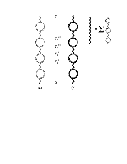
Figure 2: Diagram (a) shows $n$ Pomeron loops in series. Diagram (b) shows a series of $n$ Pomeron self mass interactions, where the bold lines represent a superposition of $n$ loops in series.

Eq. (2.6) is the scattering amplitude arising from the exchange of a bare Pomeron. According to the Schwinger-Dyson equation Braun:2005hx , the bare Pomeron propagator should be replaced by the Green’s function which is found by summing over the class of diagrams of Fig. 2. This Green’s function is found by first summing over all diagrams with $n$ consecutive loops in series shown in Fig. 2 (a), from $n=0$ to infinity. Next, the Pomeron lines themselves in Fig. 2 (a) should be replaced with the sum over loops in series which leads to Fig. 2 (b). The self mass terms in Fig. 2 (b) are “loops made of a superposition of loops”. Continuing in the same way to introduce more generations of loop series, one derives the Green’s function which is the sum over all Pomeron loop diagrams. The process which has been explained here in words, is described by the Schwinger Dyson equation introduced by M. Braun in ref. Braun:2005hx , Braun:2009sh . This expresses the full Pomeron Green function $G\left(\nu,y\right)$ in $\nu,y$-representation, as the sum over the class of diagrams in Fig. 2 as;

$$G\left(\nu,y\right)=g\left(\nu\right)-g\left(\nu\right)\int^{y}_{0}\!\!\!dy_{1}\!\int^{y_{1}}_{0}\!\!\!dy_{2}\,m\left(\nu,y_{12}\right)G\left(\nu,y_{2}\right)$$ (3.7)

where $m\left(\nu,y_{12}\right)$ is the Pomeron self mass ($y_{12}=y_{1}-y_{2}$), which sits between the rapidity values $y_{1}$ for the upper rapidity limit, and $y_{2}$ for the lower rapidity limit (see Fig. 2 (a)), and is given by the expression;

$$m\left(\nu,y_{12}\right) =\frac{1}{16}\int^{\infty}_{-\infty}\!\!\!d\nu_{1}h\left(\nu_{1}\right)G\left(\nu_{1},y_{12}\right)\!\int^{\infty}_{-\infty}\!\!\!d\nu_{2}h\left(\nu_{2}\right)G\left(\nu_{2},y_{12}\right)|\Gamma\left(\nu,\nu_{1},\nu_{2}\right)|^{2}\,e^{\left(\omega\left(\nu_{1}\right)+\omega\left(\nu_{2}\right)-\omega\left(\nu\right)\right)y_{12}}\hskip 42.67912pt$$ (3.8)

The pre-factor of $1/16$ in Eq. (3.8) divides by the order of the symmetry group, so that identical diagrams are only counted once (see ref. Miller:2009ca for a full explanation). $\Gamma\left(\nu,\nu_{1},\nu_{2}\right)$ is the triple Pomeron vertex for the splitting of the Pomeron with the conformal variable $\nu$ into two daughter Pomerons with conformal variables $\nu_{1}$ and $\nu_{2}$ which form the branches of the loop. The splitting vertex is the complex conjugate of the merging vertex, so the squared absolute value of the vertex in Eq. (3.8) is the product of the splitting and the re-merging vertex, forming the loop.

The Schwinger Dyson Eq. (3.7) forms an iterative sum, which after expanding takes the following form;

$$G\left(\nu,y\right) =g\left(\nu\right)\sum^{\infty}_{n=0}\left(-1\right)^{n}g^{n}\left(\nu\right)\prod^{n}_{i=1}\int^{y_{2}^{i+1}}_{0}\!\!\!dy_{1}^{i}\!\int^{y_{1}^{i}}_{0}\!\!\!dy_{2}^{i}\,m\left(\nu,y_{12}^{i}\right);\hskip 42.67912pty_{2}^{n+1}=y;$$ (3.9a)

$$m\left(\nu,y_{12}^{i}\right) =\frac{1}{16}\int^{\infty}_{-\infty}\!\!\!d\nu_{1}h\left(\nu_{1}\right)G\left(\nu_{1},y_{12}^{i}\right)\!\int^{\infty}_{-\infty}\!\!\!d\nu_{2}h\left(\nu_{2}\right)G\left(\nu_{2},y_{12}^{i}\right)|\Gamma\left(\nu,\nu_{1},\nu_{2}\right)|^{2}\,e^{\left(\omega\left(\nu_{1}\right)+\omega\left(\nu_{2}\right)-\omega\left(\nu\right)\right)y_{12}^{i}}\hskip 42.67912pt$$ (3.9b)

where $m\left(\nu,y_{12}^{i}\right)$ is the Pomeron self mass which sits between the rapidity values $y_{1}^{i}$ and $y_{2}^{i}$ in Fig. 2 (b), and $y^{i}_{12}=y^{i}_{1}-y^{i}_{2}$. The $G\left(\nu_{1},y_{12}^{i}\right)$ and $G\left(\nu_{2},y_{12}^{i}\right)$ in Eq. (3.9b) are the same Pomeron propagators given by the infinite Schwinger-Dyson sum of Eq. (3.9a). From this it becomes clear how plugging Eq. (3.9b) into Eq. (3.9a) generates the non-closed sum over the never ending spectrum of Pomeron loop diagrams. The integration limits are due to the upper rapidity value $y_{1}^{i}$ in Fig. 2 which cannot exceed the lower rapidity value $y_{2}^{i+1}$ of the next self mass interaction above it. The strategy for deriving a closed expression which is a solution to Eq. (3.9a) is the following.

First consider the sum over diagrams of the type shown in Fig. 2 (a), which contains $n$ Pomeron loops in series. The sum over all such diagrams from $n=0$ to infinity is described by the Schwinger Dyson Eq. (3.9a) by replacing $m\left(\nu,y_{12}^{i}\right)$ with the Pomeron loop $m_{0}\left(\nu,y_{12}^{i}\right)$ which yields;

$$G_{0}\left(\nu,y|\mbox{{Fig.~{}\ref{fren}} (a)}\right) =g\left(\nu\right)\sum^{\infty}_{n=0}\left(-1\right)^{n}g^{n}\left(\nu\right)\prod^{n}_{i=1}\int^{y_{2}^{i+1}}_{0}\!\!\!dy_{1}^{i}\!\int^{y_{1}^{i}}_{0}\!\!\!dy_{2}^{i}\,m_{0}\left(\nu,y_{12}^{i}\right)$$ (3.10a)

$$m_{0}\left(\nu,y_{12}^{i}\right) =\frac{1}{16}\int^{\infty}_{-\infty}\!\!\!d\nu_{1}h\left(\nu_{1}\right)g\left(\nu_{1}\right)\!\int^{\infty}_{-\infty}\!\!\!d\nu_{2}h\left(\nu_{2}\right)g\left(\nu_{2}\right)|\Gamma\left(\nu,\nu_{1},\nu_{2}\right)|^{2}\,e^{\left(\omega\left(\nu_{1}\right)+\omega\left(\nu_{2}\right)-\omega\left(\nu\right)\right)y_{12}^{i}}\hskip 28.45274pt$$ (3.10b)

where $m_{0}\left(\nu,y_{12}^{i}\right)$ is found from Eq. (3.9b) by replacing the renormalized propagators $G\left(\nu_{1},y_{12}^{i}\right)$ and $G\left(\nu_{2},y_{12}^{i}\right)$, with the bare propagators $g\left(\nu_{1}\right)$ and $g\left(\nu_{2}\right)$. From the Korchemsky expression for the triple Pomeron vertex Korchemsky:1997fy , it was found in ref. Miller:2009ca , Miller:2009 that there are two main contributions to the triple Pomeron vertex which are given by the following asymptotes;

$$|\Gamma\left(i\nu=\frac{1}{2},i\nu_{1}=0,i\nu_{2}=0\right)|^{2}\!=\!\frac{\left(4\pi\right)^{6}\bar{\alpha}_{s}^{4}}{N_{c}^{4}}\frac{1}{1/4+\nu^{2}}$$ (3.11a)

$$|\Gamma\left(\nu,i\nu_{1}=\frac{1}{2},i\nu_{2}=\frac{1}{2}\right)|^{2}\!=\!\frac{1}{2}\left(4\pi\right)^{6}\bar{\alpha}_{s}^{4}\left(1-\frac{1}{N_{c}^{2}}\right)^{2}\!\!\chi\left(\nu\right)\!\left(\frac{1}{4}+\nu^{2}\right)^{3}\!\!\frac{1-i\nu_{1}-i\nu_{2}}{\left(1/2-i\nu_{1}\right)^{2}\left(1/2-i\nu_{2}\right)^{2}}\hskip 45.52458pt$$ (3.11b)

$$\chi\left(\nu\right)\!=\!\Re e\left(\psi\left(1\right)-\psi\left(\frac{1}{2}+i\nu\right)\right)$$ (3.11c)

Eq. (3.11a) leads to the contribution to the Pomeron loop amplitude of Eq. (3.10b) which is equivalent to $2$ non interacting Pomerons, with renormalized Pomeron vertices. This particular contribution to $m_{0}\left(\nu,y_{12}^{i}\right)$ gives a vanishing result for $n>1$ in Eq. (3.10a). This makes sense since Eq. (3.10a) describes the sum over $n$ Pomeron loops in series shown in Fig. 2 (a). Therefore the phenomena where the branches of the loop span the entire rapidity gap between the projectile and target to become 2 independent partons, cannot occur with more than 1 loop in series. With this in mind the contribution to the vertex of Eq. (3.11a) is postponed until the non interacting Pomeron solution is discussed later on in section 4. For now, inserting the asymptote of Eq. (3.11b) into Eq. (3.10b), and then introducing the definitions given in Eq. (2.4) (where $g\left(\nu\right)$ can be cast as $1/16\left(1/2+i\nu\right)^{2}\left(1/2-i\nu\right)^{2}\,$ );

$$m_{0}\left(\nu,y_{12}^{i}\right) =\frac{\pi^{6}}{2}\!\!\left(1-\frac{1}{N_{c}^{2}}\right)^{2}\!\!\left(\frac{1}{4}+\nu^{2}\right)^{3}\!\!\chi\left(\nu\right)$$

$$\times\int^{\infty}_{-\infty}\!\!\frac{d\nu_{1}\,\nu_{1}^{2}}{\left(\frac{1}{2}+i\nu_{1}\right)^{2}\left(\frac{1}{2}-i\nu_{1}\right)^{4}}\!\int^{\infty}_{-\infty}\!\!\frac{d\nu_{2}\,\nu_{2}^{2}\left(1-i\nu_{1}-i\nu_{2}\right)}{\left(\frac{1}{2}+i\nu_{2}\right)^{2}\left(\frac{1}{2}-i\nu_{2}\right)^{4}}\,e^{\left(\omega\left(\nu_{1}\right)+\omega\left(\nu_{2}\right)-\omega\left(\nu\right)\right)y_{12}^{i}}$$

The $\nu_{1},\nu_{2}$ integrals are solved by closing the contour over the upper half plane and summing over the residues at $i\nu_{1},i\nu_{2}=1/2$, taking into account the poles which stem from $\omega\left(\nu_{1,2}\right)\xrightarrow{i\nu_{1,2}\to 1/2}-\bar{\alpha}_{s}/\left(1/2-i\nu_{1,2}\right)$ such that Eq. (3) becomes

$$m_{0}\left(\nu,y_{12}^{i}\right) =\frac{\pi^{6}}{2}\!\left(1-\frac{1}{N_{c}^{2}}\right)^{2}\!\!\left(\frac{1}{4}+\nu^{2}\right)^{3}\!\!\chi\left(\nu\right)\oint_{C}\frac{d\nu_{1}\,\nu_{1}^{2}}{\left(\frac{1}{2}+i\nu_{1}\right)^{2}\!\left(\frac{1}{2}-i\nu_{1}\right)^{4}}\oint_{C}\frac{d\nu_{2}\,\nu_{2}^{2}\left(1-i\nu_{1}-i\nu_{2}\right)}{\left(\frac{1}{2}+i\nu_{2}\right)^{2}\!\left(\frac{1}{2}-i\nu_{2}\right)^{4}}$$ (3.13)

$$\times e^{\left(-\bar{\alpha}_{s}\left(1/2-i\nu_{1}\right)^{-1}-\bar{\alpha}_{s}\left(1/2-i\nu_{2}\right)^{-1}-\omega\left(\nu\right)\right)y_{12}^{i}}$$

$$=\frac{\pi^{6}}{2}\left(1-\frac{1}{N_{c}^{2}}\right)^{2}\!\!\left(\frac{1}{4}+\nu^{2}\right)^{3}\!\!\chi\left(\nu\right)\oint_{C}\frac{d\nu_{1}\,\nu_{1}^{2}}{\left(\frac{1}{2}+i\nu_{1}\right)^{2}\left(\frac{1}{2}-i\nu_{1}\right)^{2}}\left(\frac{-1}{\bar{\alpha}_{s}}\frac{d}{dy_{12}^{i}}\right)^{2}e^{-\bar{\alpha}_{s}\left(1/2-i\nu_{1}\right)^{-1}y_{12}^{i}}$$

$$\times\oint_{C}\frac{d\nu_{2}\,\nu_{2}^{2}\left(1-i\nu_{1}-i\nu_{2}\right)}{\left(\frac{1}{2}+i\nu_{2}\right)^{2}\left(\frac{1}{2}-i\nu_{2}\right)^{4}}\,e^{\left(-\bar{\alpha}_{s}\left(1/2-i\nu_{2}\right)^{-1}-\omega\left(\nu\right)\right)y_{12}^{i}}$$

It is instructive to change the $\nu_{1}$ integration variable to $u=\bar{\alpha}_{s}/\left(1/2-i\nu_{1}\right)+\bar{\alpha}_{s}/\left(1/2-i\nu_{2}\right)$, such that the jacobian cancels the remaining singularity which stems from $\left(1/2-i\nu_{1}\right)^{-2}$ in Eq. (3.13). Integrating over $u$ yields the derivative of the Dirac delta function $2\pi i\delta^{(2)}\left(y_{1}^{i}-y_{2}^{i}\right)$. After taking the residue at $i\nu_{1}=1/2$ the $\nu_{2}$ integral reduces to $\oint_{C}d\nu_{2}\,\nu_{2}^{2}/\left(\frac{1}{2}+i\nu_{2}\right)^{2}\left(\frac{1}{2}-i\nu_{2}\right)^{3}=2\pi i/4$. Over all, after re-arranging the order of derivatives so that there are no derivatives of the delta function in the integrand, one finds for the Pomeron loop amplitude the following expression;

$$m_{0}\left(\nu,y_{12}^{i}\right) =a\left(\frac{1}{4}+\nu^{2}\right)^{3}\chi\left(\nu\right)\omega^{2}\left(\nu\right)e^{-\omega\left(\nu\right)y_{12}^{i}}\delta\left(y_{1}^{i}-y_{2}^{i}\right);\hskip 28.45274pta=\bar{\alpha}_{s}\left(1-\frac{1}{N_{c}^{2}}\right)^{2}$$ (3.14)

Finally inserting Eq. (3.14) into Eq. (3.10a), the integrations over the rapidity variables are trivially solved thanks to the Dirac delta function. Thus one derives the following expression for the sum over the class of diagrams of Fig. 2 (a) with $n$ consecutive loops ;

$$G_{0}\left(\nu,y|\mbox{{Fig.~{}\ref{fren}} (a)}\right) =g\left(\nu\right)\sum^{\infty}_{n=0}\frac{\left(-1\right)^{n}}{n!}\left(g\left(\nu\right)\,a\,\left(1/4+\nu^{2}\right)^{3}\chi\left(\nu\right)\omega^{2}\left(\nu\right)\,y\,\right)^{n}$$ (3.15)

$$=g\left(\nu\right)\exp\left(-\frac{a}{16}\left(\frac{1}{4}+\nu^{2}\right)\chi\left(\nu\right)\omega^{2}\left(\nu\right)y\right)$$

Substituting for the bare propagator $g\left(\nu\right)$ that appears in Eq. (2.3), the renormalized one derived in Eq. (3.15), leads to the scattering amplitude which is equivalent to the replacement;

$$\omega\left(\nu\right)\to\widetilde{\omega}\left(\nu\right)=\omega\left(\nu\right)+\zeta\left(\nu\right);\hskip 28.45274pt\zeta\left(\nu\right)=-\frac{a}{16}\left(\frac{1}{4}+\nu^{2}\right)\chi\left(\nu\right)\omega^{2}\left(\nu\right)$$ (3.16)

Therefore the sum over the class of diagrams in Fig. 2 (a) leads directly to the renormalized Pomeron intercept given by Eq. (3.16). Phrased differently, the sum over the class of diagrams of Fig. 2 (a) is found by replacing $\omega\left(\nu\right)$ in Eq. (2.3) with Eq. (3.16). The bold lines in Fig. 2 (b), represent the sum over the class of diagrams in Fig. 2 (a). As such Fig. 2 (b) is a string of loops, where the bold lines which form the loops are themselves a string of loops. The bold lines are reggeons, with the renormalized intercept $\widetilde{\omega}\left(\nu\right)$ derived in Eq. (3.16). With this in mind, the sum over the class of diagrams of Fig. 2 (b) is derived from Eq. (3.10), by replacing the intercepts $\omega\left(\nu_{1}\right)$ and $\omega\left(\nu_{2}\right)$ with $\widetilde{\omega}\left(\nu_{1}\right)$ and $\widetilde{\omega}\left(\nu_{2}\right)$ found in Eq. (3.16), which yields;

$$G\left(\nu,y|\mbox{{Fig.~{}\ref{fren}} (b)}\right) =g\left(\nu\right)\sum^{\infty}_{n=0}\left(-1\right)^{n}g^{n}\left(\nu\right)\prod^{n}_{i=1}\int^{y_{2}^{i+1}}_{0}\!\!\!dy_{1}^{i}\!\int^{y_{1}^{i}}_{0}\!\!\!dy_{2}^{i}\,m\left(\nu,y_{12}^{i}\right);$$ (3.17a)

$$m\left(\nu,y_{12}^{i}\right) =\frac{1}{16}\int^{\infty}_{-\infty}\!\!\!d\nu_{1}h\left(\nu_{1}\right)g\left(\nu_{1}\right)\!\int^{\infty}_{-\infty}\!\!\!d\nu_{2}h\left(\nu_{2}\right)g\left(\nu_{2}\right)|\Gamma\left(\nu,\nu_{1},\nu_{2}\right)|^{2}\,e^{\left(\widetilde{\omega}\left(\nu_{1}\right)+\widetilde{\omega}\left(\nu_{2}\right)-\omega\left(\nu\right)\right)y_{12}^{i}}\hskip 42.67912pt$$ (3.17b)

Following the same arguments used above, the integrations in Eq. (3.17b) are solved by closing the $\nu_{1},\nu_{2}$ contours over the upper half plane and summing over the residues at $i\nu_{1},i\nu_{2}=1/2$. After introducing the definitions given in Eq. (2.4) and taking into account the singularities that stem from the triple Pomeron vertex of Eq. (3.11b), and the asymptotes;

$$\omega\left(\nu\right)\xrightarrow{i\nu\to 1/2}\frac{-\bar{\alpha}_{s}}{\frac{1}{2}-i\nu};\hskip 14.22636pt\zeta\left(\nu\right)\xrightarrow{i\nu\to 1/2}\frac{a}{16}\frac{\bar{\alpha}_{s}^{2}}{\left(\frac{1}{2}-i\nu\right)^{2}}$$ (3.18)

Eq. (3.17b) becomes;

$$m\left(\nu,y_{12}^{i}\right) =\frac{\pi^{6}}{2}\!\left(1-\frac{1}{N_{c}^{2}}\right)^{2}\!\!\left(\frac{1}{4}+\nu^{2}\right)^{3}\!\!\chi\left(\nu\right)$$ (3.19)

$$\times\oint_{C}\frac{d\nu_{1}\,\nu_{1}^{2}}{\left(\frac{1}{2}+i\nu_{1}\right)^{2}\left(\frac{1}{2}-i\nu_{1}\right)^{4}}\exp\left(\frac{-\bar{\alpha}_{s}}{\frac{1}{2}-i\nu_{1}}y_{12}^{i}+\frac{a}{16}\frac{\bar{\alpha}_{s}^{2}}{\left(\frac{1}{2}-i\nu_{1}\right)^{2}}y_{12}^{i}\right)$$

$$\times\oint_{C}\frac{d\nu_{2}\,\nu_{2}^{2}\left(1-i\nu_{1}-i\nu_{2}\right)}{\left(\frac{1}{2}+i\nu_{2}\right)^{2}\left(\frac{1}{2}-i\nu_{2}\right)^{4}}\,e^{\left(\widetilde{\omega}\left(\nu_{2}\right)-\omega\left(\nu\right)\right)y_{12}^{i}}$$

$$=\frac{\pi^{6}}{2}\!\left(1-\frac{1}{N_{c}^{2}}\right)^{2}\!\!\left(\frac{1}{4}+\nu^{2}\right)^{3}\!\!\!\chi\left(\nu\right)\!$$

$$\times\oint_{C}\!\frac{d\nu_{1}\,\nu_{1}^{2}}{\left(\frac{1}{2}+i\nu_{1}\right)^{2}\left(\frac{1}{2}-i\nu_{1}\right)^{2}}\left(\frac{-1}{\bar{\alpha}_{s}}\frac{d}{dy_{12}^{i}}\right)^{2}\!\exp\left(\frac{a}{16}y_{12}^{i}\frac{d^{2}}{d^{2}y_{12}^{i}}\right)\!\exp\left(\frac{-\bar{\alpha}_{s}}{\frac{1}{2}-i\nu_{1}}y_{12}^{i}\right)$$

$$\times\oint_{C}\frac{d\nu_{2}\,\nu_{2}^{2}\left(1-i\nu_{1}-i\nu_{2}\right)}{\left(\frac{1}{2}+i\nu_{2}\right)^{2}\left(\frac{1}{2}-i\nu_{2}\right)^{4}}\,e^{\left(\widetilde{\omega}\left(\nu_{2}\right)-\omega\left(\nu\right)\right)y_{12}^{i}}\hskip 42.67912pt$$

Changing the integration variable to $w=\bar{\alpha}_{s}/\left(1/2-i\nu_{1}\right)+\widetilde{\omega}\left(\nu_{2}\right)$ and integrating over $w$ yields the Dirac delta function $2\pi i\delta\left(y_{1}^{i}-y_{2}^{i}\right)$, acted on by the derivatives with respect to $y_{12}^{i}$ which appear in the integrand. After taking the residue at $i\nu_{1}=1/2$ the $\nu_{2}$ integral reduces to $\oint_{C}d\nu_{2}\,\nu_{2}^{2}/\left(\frac{1}{2}+i\nu_{2}\right)^{2}\left(\frac{1}{2}-i\nu_{2}\right)^{3}=2\pi i/4$. After rearranging the order of derivatives so that there is no derivative of the Dirac Delta function in the final expression;

$$m\left(\nu,y_{12}^{i}\right) =a\left(\frac{1}{4}+\nu^{2}\right)^{3}\chi\left(\nu\right)\omega^{2}\left(\nu\right)\,e^{-\omega\left(\nu\right)y_{12}^{i}}\left\{\exp\left(-\frac{a}{16}\omega^{2}\left(\nu\right)y_{12}^{i}\right)+\phi\left(\nu\right)\right\}\delta\left(y_{1}^{i}-y_{2}^{i}\right)$$ (3.20a)

$$\phi\left(\nu\right) =\frac{1-\sqrt{1-4\varphi\left(\nu\right)}-2\varphi\left(\nu\right)}{2\sqrt{1-4\varphi\left(\nu\right)}\varphi^{2}\left(\nu\right)};\hskip 14.22636pt\varphi\left(\nu\right)=\frac{a}{16}\omega\left(\nu\right)$$ (3.20b)

Finally inserting Eq. (3.20a) into Eq. (3.17a) and evaluating all the integrations over the rapidity variables leads to the following result for the sum over the class of diagrams shown in Fig. 2 (b);

$$G\left(\nu,y|\mbox{{Fig.~{}\ref{fren}} (b)}\right)=g\left(\nu\right)\exp\left\{-\frac{a}{16}\left(\frac{1}{4}+\nu^{2}\right)\chi\left(\nu\right)\omega^{2}\left(\nu\right)\left(1+\phi\left(\nu\right)\right)\,y\,\right\}$$ (3.21)

Using exactly the same arguments which led to Eq. (3.16), the sum over the class of diagrams with $n$ consecutive self mass terms shown in Fig. 2 (b), is achieved by replacing $\omega\left(\nu\right)$ that appears in Eq. (2.3), with the following renormalized Pomeron intercept;

$$\omega\left(\nu\right)\to\widetilde{\widetilde{\omega}}\left(\nu\right)=\omega\left(\nu\right)+\zeta\left(\nu\right)\left(1+\phi\left(\nu\right)\right)$$ (3.22)

If the same treatment is repeated and another deeper level of loops are introduced, the Pomeron intercepts $\omega\left(\nu_{1}\right)$ and $\omega\left(\nu_{2}\right)$ in Eq. (3.10b) are replaced by Eq. (3.22). The $\nu_{1},\nu_{2}$ integrals are solved in the same way by closing the contour over the upper half plane and summing over the residues at $i\nu_{1},i\nu_{2}=1/2$. Fortunately, $\phi\left(\nu_{1,2}\right)$ vanishes as $i\nu_{1,2}\to 1/2$, so it gives no contribution to the sum over residues. This means that the steps from Eq. (3.17) to Eq. (3.21) are identical, and the same expression of Eq. (3.22) for the renormalized Pomeron intercept is derived. Therefore every time a deeper level of loops is introduced, one always arrives at Eq. (3.22) for the renormalization of the Pomeron intercept. Therefore the following expression derived in Eq. (3.21)

$$G\left(\nu,y\right)=g\left(\nu\right)\exp\left\{-\frac{a}{16}\left(\frac{1}{4}+\nu^{2}\right)\chi\left(\nu\right)\omega^{2}\left(\nu\right)\left(1+\phi\left(\nu\right)\right)\,y\,\right\}$$ (3.23)

is the solution to the Schwinger Dyson equation Eq. (3.9a) which describes the sum over the class of Pomeron loop diagrams in Fig. 2. The solution is equivalent to the replacement of the Pomeron intercept $\omega\left(\nu\right)$, with the renormalized Pomeron intercept $\widetilde{\widetilde{\omega}}\left(\nu\right)$ derived in Eq. (3.22).

4 The non interacting Pomeron solution

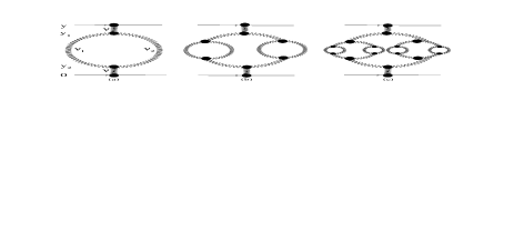
Figure 3: The special class of symmetric Pomeron loop diagrams taken into account in the sum over Pomeron loops. (a) is the diagram with $N=1$ generation of loops, (b) has $N=2$ generations of loops and (c) has $N=3$ generations of loops.

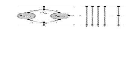
Figure 4: The $N$ generation diagram which stems from the simple loop giving birth to two sets of $N-1$ generations of loops, is equivalent to the diagram of $2^{N}$ non interacting Pomerons with renormalized Pomeron vertices.

The next part of the discussions is focussed on the non interacting Pomeron solution, which stems from diagrams of the type shown in Fig. 4. Loops which become non interacting Pomerons do not contribute to consecutive loops in Fig. 2 (a), because the phenomena where the branches of the loop stretch and span the whole rapidity gap between the projectile and target, can’t happen for more than one loop in series. Therefore this solution cannot be treated in the context of the Schwinger Dyson Eq. (3.9a) for $n>1$, and requires a separate approach. Using the same conventions, the scattering amplitude of Fig. 4 (a) is given by the expression;

$$A_{(1)}\left(y|\mbox{{Fig.~{}\ref{fsopl}} (a)}\right)=\frac{\alpha_{s}^{2}}{4}\!\int^{\infty}_{-\infty}\!\!\!d\nu h\left(\nu\right)g^{2}\left(\nu\right)e^{\omega\left(\nu\right)y}m_{(1)}\left(\nu,y\right)E_{\nu}E^{\prime}_{-\nu}$$ (4.24a)

$$m_{(1)}\left(\nu,y\right)=\frac{1}{16}\int^{\infty}_{-\infty}\!\!\!d\nu_{1}h\left(\nu_{1}\right)g\left(\nu_{1}\right)\int^{\infty}_{-\infty}\!\!\!d\nu_{2}h\left(\nu_{2}\right)g\left(\nu_{2}\right)|\Gamma\left(\nu|\nu_{1},\nu_{2}\right)|^{2}$$ (4.24b)

$$\times\int^{y}_{0}dy_{1}\!\int^{y_{1}}_{0}dy_{2}e^{\left(\omega\left(\nu_{1}\right)+\omega\left(\nu_{2}\right)-\omega\left(\nu\right)\right)y_{12}}$$

where $y_{12}=y_{1}-y_{2}$ is the rapidity gap which the loop fills (see Fig. 4 (a)). Now inserting the asymptote of Eq. (3.11a) for the triple Pomeron vertex for the region where $\nu_{1},\nu_{2}$ are close to zero, one can substitute for the BFKL eigenfunctions $\omega\left(\nu_{1}\right)$ and $\omega\left(\nu_{2}\right)$ the expansion of Eq. (2.5) and integrate over $\nu_{1}$ and $\nu_{2}$ using the method of steepest descents, which gives the expression Miller:2009ca , Miller:2009 ;

$$m_{(1)}\left(\nu,y\right) =\frac{b}{\left(1/4+\nu^{2}\right)}\int^{y}_{0}dy_{1}\!\int^{y_{1}}_{0}dy_{2}\frac{e^{\left(2\omega\left(0\right)-\omega\left(\nu\right)\right)y_{12}}}{y_{12}^{3}};\hskip 28.45274ptb=\frac{2^{10}\bar{\alpha}_{s}^{4}}{N_{c}^{4}\pi\left(\omega^{\prime\prime}\left(0\right)\right)^{3}}\,.$$ (4.25)

Inserting Eq. (4.25) back into Eq. (4.24a), the $\nu$ integration can be solved by closing the contour over the upper half plane and summing over the residues at $i\nu=1/2$, taking into account the singularity which stems from $\omega\left(\nu\right)$ given in Eq. (3.18). This leads to the following contribution to the scattering amplitude Miller:2009ca , Miller:2009 ;

$$A_{(1)}\left(y|\mbox{{Fig.~{}\ref{fsopl}} (a)}\right) =\frac{\bar{\alpha}_{s}b}{2^{9}\pi N_{c}^{2}}y\left(\frac{-1}{\bar{\alpha}_{s}}\frac{d}{dy}\right)^{3}\frac{e^{2\omega\left(0\right)y}}{y^{3}}$$ (4.26)

Eq. (4.26) is equivalent to 2 non interacting Pomerons, with renormalized Pomeron vertices. As explained above, Fig. 4 (b) stems from Fig. 4 (a) when each branch of the loop gives birth to a secondary loop leading to the two “second generation” of loops in Fig. 4 (b). In the same way when the second generation loops in Fig. 4 (b) each give birth to two loops, this leads to 4 “third generation” of loops in Fig. 4 (c). Continuing with this evolution, the entire spectrum of symmetric $N$ generation diagrams can be generated for all $N$ . The scattering amplitude with $N$ generations of loops shown in Fig. 4 is the generalization of Eq. (4.24a), namely Miller:2009ca , Miller:2009 ;

$$A_{(N)}\left(y|\mbox{{Fig.~{}\ref{fpictN1}}}\right) =\frac{\alpha_{s}^{2}}{4}\int^{\infty}_{-\infty}\!\!\!d\nu h\left(\nu\right)g^{2}\left(\nu\right)e^{\omega\left(\nu\right)y}m_{(N)}\left(\nu,y\right)E_{\nu}E^{\prime}_{-\nu}$$ (4.27)

where $m_{(N)}\left(\nu,y\right)$ is the contribution of the $N$ generations of loops in Fig. 4. In refs. Miller:2009ca , Miller:2009 a detailed explanation of how to calculate $m_{(N)}\left(\nu,y\right)$ was given. This is based on the observation that Fig. 4 is equivalent to the simple loop diagram of Fig. 4 (a) when each branch in the loop gives birth to a set of $N-1$ generations of loops. This means that to write the expression for $m_{(N)}\left(\nu,y\right)$, all that is needed is to modify the propagators for the branches of the loop in the expression of Eq. (4.24b) as;

$$g\left(\nu_{1}\right)\to g\left(\nu_{1}\right)m_{(N-1)}\left(\nu_{1},y_{12}\right)g\left(\nu_{1}\right);\hskip 14.22636ptg\left(\nu_{2}\right)\to g\left(\nu_{2}\right)m_{(N-1)}\left(\nu_{2},y_{12}\right)g\left(\nu_{2}\right)$$ (4.28)

After implementing Eq. (4.28) in Eq. (4.24b), one arrives at the following amplitude for the set of $N$ generations of loops;

$$m_{(N)}\left(\nu|y,\delta y_{H}\right) =\frac{1}{16}\int^{\infty}_{-\infty}\!\!\!d\nu_{1}h\left(\nu_{1}\right)g\left(\nu_{1}\right)\int^{\infty}_{-\infty}\!\!\!d\nu_{2}h\left(\nu_{2}\right)g\left(\nu_{2}\right)|\Gamma\left(\nu|\nu_{1},\nu_{2}\right)|^{2}$$

$$\times\int^{y}_{0}dy_{1}\!\int^{y_{1}}_{0}dy_{2}e^{\left(\omega\left(\nu_{1}\right)+\omega\left(\nu_{2}\right)-\omega\left(\nu\right)\right)y_{12}}m_{(N-1)}\left(\nu_{1},y_{12}\right)m_{(N-1)}\left(\nu_{2},y_{12}\right)$$

Eq. (4) forms an iterative expression. Using the technique of proof by induction, the following formula derived in refs. Miller:2009ca , Miller:2009 for Eq. (4) can be proved;

$$m_{(N)}\left(\nu,y\right) =\frac{\left(bb^{\,\prime}\right)^{2^{[N-1]}}}{b^{\,\prime}}\left(\frac{1}{4}+\nu^{2}\right)^{3}\chi\left(\nu\right)\int^{y}_{0}dy_{1}\int^{y_{1}}_{0}dy_{2}\,y_{12}^{2^{[N-1]}-1}\left\{\!\left(\frac{-1}{\bar{\alpha}_{s}}\frac{d}{dy_{12}}\right)^{3}\!\frac{e^{2\omega\left(0\right)y_{12}}}{y_{12}^{3}}\!\right\}^{2^{[N-1]}}$$ (4.30a)

$$b =\frac{2^{10}\bar{\alpha}_{s}^{4}}{N_{c}^{4}\pi[\omega^{\,\prime\prime}\left(0\right)]^{3}};\hskip 14.22636ptb^{\prime}=\frac{\bar{\alpha}_{s}^{2}}{2^{11}}\left(1-\frac{1}{N_{c}^{2}}\right)^{2}.$$ (4.30b)

Finally after inserting Eq. (4.30) into Eq. (4.27), one finds the following scattering amplitude for the diagram of Fig. 4 with $N$ generations of loops;

$$A_{(N)}\left(y|\mbox{{Fig.~{}\ref{fpictN1}}}\right) =\frac{\bar{\alpha}_{s}\,}{2^{9}N_{c}^{2}\pi}\frac{\left(bb^{\prime}\right)^{2^{[N-1]}}}{b^{\prime}}y^{2^{[N-1]}}\left\{\!\!\left(\frac{-1}{\bar{\alpha}_{s}}\frac{d}{dy}\right)^{3}\!\!\frac{e^{2\omega\left(0\right)y}}{y^{3}}\!\!\right\}^{2^{[N-1]}}$$ (4.31)

Eq. (4.31) is equivalent to $2^{N}$ non interacting Pomerons, with renormalized Pomeron vertices shown pictorially in Fig. 4. This follows from the observation that Eq. (4.31) can be recast in the form;

$$A_{(N)}\left(y|\mbox{{Fig.~{}\ref{fpictN1}}}\right)\equiv\kappa_{\mbox{\tiny{\it(N)}}}\,e^{2^{N}\omega\left(0\right)y}$$ (4.32)

where the coefficient $\kappa_{\mbox{\tiny{\it(N)}}}$ contains the set of renormalized Pomeron vertices. Eq. (4.31) describes the scattering amplitude with $2^{N-1}$ loops, which is equivalent to $2^{N}$ non interacting Pomerons. This formula can be generalized to the scattering amplitude of the symmetric diagram which contains $n$ loops, or equivalently $2n$ non interacting Pomerons, namely;

$$A_{(n)}\left(y\right) =\frac{\bar{\alpha}_{s}\,}{2^{9}N_{c}^{2}\pi}\frac{\left(bb^{\,\prime}\right)^{n}}{b^{\,\prime}}y^{n}\left\{\!\!\left(\frac{-1}{\bar{\alpha}_{s}}\frac{d}{dy}\right)^{3}\!\!\frac{e^{2\omega\left(0\right)y}}{y^{3}}\!\!\right\}^{n}$$ (4.33)

The sum over the complete set of symmetric Pomeron loop diagrams, is achieved by evaluating the sum $\sum^{\infty}_{n=0}A_{(n)}\left(y\,|\,\mbox{{Eq.~{}(\ref{AN3generalized})}}\right)$. In the outcome formula, the intercept $\omega\left(0\right)$ should be replaced with $\widetilde{\widetilde{\omega}}\left(0\right)$ of Eq. (3.22). This leads to the sum over diagrams with independent Pomeron exchanges, where the Pomerons are replaced by the superposition of loop series shown in Fig. 2, described by the Schwinger Dyson equation. In this formalism the full sum over symmetric Pomeron loop diagrams is given by;

$$\sum^{\infty}_{n=1}A_{(n)}\left(y\right) =\frac{\bar{\alpha}_{s}\,}{2^{9}N_{c}^{2}\pi}yb\left(\frac{-1}{\bar{\alpha}_{s}}\frac{d}{dy}\right)^{3}\!\!\frac{e^{2\widetilde{\widetilde{\omega}}\left(0\right)y}}{y^{3}}$$

$$\overline{\hskip 11.38092pt1+bb^{\,\prime}y\,\left(\frac{-1}{\bar{\alpha}_{s}}\frac{d}{dy}\right)^{3}\!\!\frac{e^{2\widetilde{\widetilde{\omega}}\left(0\right)y}}{y^{3}}\hskip 11.38092pt}$$

5 Results

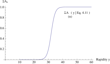
Figure 5: The energy dependence of the sum over symmetric Pomeron loop diagrams $\sum^{\infty}_{n=1}A_{(n)}\left(y|\mbox{{Eq.~{}(\ref{sumoverPomeronloops})}}\right)$

The energy dependence of the sum over Pomeron loop diagrams is shown in Fig. 5. The curve approaches the black disk limit, so that unitarity is preserved. If the bare Pomeron intercept $\omega\left(0\right)$ is used in Eq. (4) instead of the renormalized one, the graph of Fig. 5 is unaffected. This indicates that the dominant contribution to the sum over Pomeron loop diagrams comes from the diagrams which are equivalent to non interacting Pomerons, with renormalized Pomeron vertices. The class of diagrams of Fig. 2 leading to the renormalized Pomeron intercept give a negligible contribution in comparison.

The formula of Eq. (4) requires explanation. It is tempting to think that Eq. (4) is the scattering amplitude, however a closer look reveals that this formula is still just the sum over a special class of loop diagrams, as will now be explained.

6 Conclusions and discussion

The following discussion is a summary of the formalism adopted in this paper, for the summation of Pomeron loops. There are two distinct ways of summing over Pomeron loops, and both methods must be taken into account, namely;

1. The sum over the class of loops in series of Fig. 2, using the Schwinger Dyson Eq. (3.9). The asymptote for the vertex of Eq. (3.11b) contributes to the Schwinger Dyson sum, whereas the asymptote of Eq. (3.11a) gives a vanishing contribution for $n>1$. The Pomeron loop summation generated by the Schwinger Dyson sum, provides the renormalized Pomeron intercept derived in Eq. (3.22).

2. The sum over the symmetric class of loops in Fig. 4, using the vertex of Eq. (3.11a). This leads to the sum over even numbers of non interacting Pomerons, with renormalized Pomeron vertices. The symmetric nature of the loops in Fig. 4, leads to even numbers of independent Pomerons. For example taking all loop branches outside in Fig. 4 (b), leaves 4 independent Pomerons.

The two asymptotic expressions for the triple Pomeron vertex in Eq. (3.11), lead to the above two entirely different types of loop summation. It should be stressed, that the above two treatments do not lead to the same result, and the scattering amplitude requires taking into account both methods. The non interacting Pomeron solution (2), originates from the loops in Fig. 4 stretching in rapidity space until they fill up the gap between the projectile and target, and therefore become independent Pomeron exchanges. This phenomena does not occur for the loops in series shown in Fig. 2, since the loop cannot become non interacting Pomerons, when there is more than one loop in series. The only class of diagram which can yield non interacting Pomerons, is the special class of loops shown in Fig. 4 (a), and the only asymptote for the vertex which can yield non interacting Pomerons is Eq. (3.11a). Hence, the non interacting Pomeron solution requires a separate treatment from the Schwinger Dyson equation.

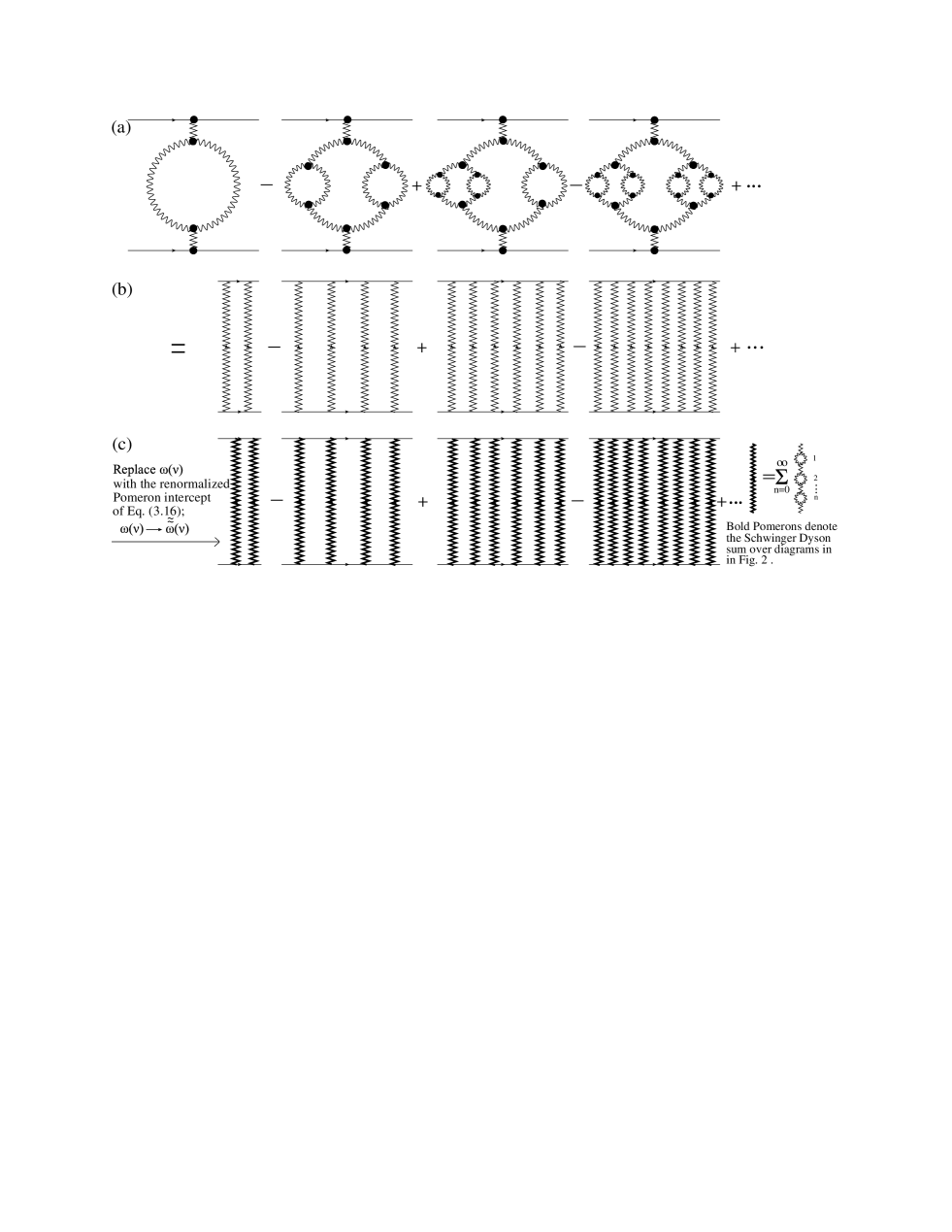
Figure 6: The process which leads to the formula of Eq. (4). Summing over the symmetric class of loops in (a), leads to the sum over even numbers of non interacting Pomerons shown in (b). Then replace the bare Pomerons with bold Pomerons, where bold Pomerons label the Schwinger Dyson sum over the class of loops in series shown in Fig. 2. The Schwinger Dyson sum renormalizes the Pomeron, by replacing the Pomeron intercept with the renormalized Pomeron intercept $\widetilde{\widetilde{\omega}}\left(\nu\right)$ of Eq. (3.22). This leads to the sum over even numbers of independent bold Pomerons in (c), that are renormalized in the framework of the Schwinger Dyson equation.

The result of Eq. (4) includes both types of summation over Pomeron loops. Fig. 6 shows a picture for the derivation of Eq. (4). It is instructive to first consider the class of loops in Fig. 6 (a). As explained in section 4, the summation over the class of loops in Fig. 6 (a) is equivalent to the sum over diagrams with an even number of non interacting Pomerons, shown in Fig. 6 (b). Next, replace the bare Pomerons with Pomerons which are renormalized by the Schwinger Dyson sum. This means that for each of the non interacting Pomerons in Fig. 6 (b), replace it with the sum over loops in series shown in Fig. 2, generated by the Schwinger Dyson equation. This is achieved by replacing the bare Pomeron intercept $\omega\left(\nu\right)$, with the renormalized intercept $\widetilde{\widetilde{\omega}}\left(\nu\right)$ derived in Eq. (3.22). This leads to the diagram of Fig. 6 (c), where the bold Pomerons label the above described renormalized Pomerons with the intercept $\widetilde{\widetilde{\omega}}\left(\nu\right)$.

The end result of Fig. 6 (c) is a true description of Eq. (4), namely the sum over diagrams with an even number of independent Pomeron exchanges, which are renormalized in the context of the Schwinger Dyson equation. The formula of Eq. (4) does not include the bare scattering amplitude of Fig. 1 given by Eq. (2.6). The complete scattering amplitude which includes the loop corrections shown in Fig. 6 is found by adding to Eq. (4), the bare scattering amplitude of Eq. (2.6). This would lead to a divergent result which violates unitarity. The only remedy for this problem, is to repeat the procedure shown in Fig. 6, for the non-symmetric class of diagrams shown in Fig. 7. Although the diagrams of Fig. 7 have been included in the Schwinger Dyson sum, this was performed using the vertex of Eq. (3.11b). The approach here, is instead to use the vertex of Eq. (3.11a) to sum over the non symmetric diagrams in Fig. 7. This will lead to the sum over odd numbers of non interacting Pomerons, that do not contribute to the Schwinger Dyson sum.

.

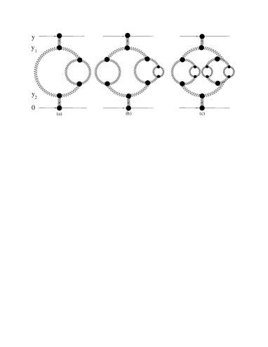
Figure 7: Examples of non symmetric Pomeron loop diagrams.

This stems from the non symmetric nature of the loops in Fig. 7, where for example taking all branches of the loops in Fig. 7 (a) outside, reduces the diagram to 3 independent Pomeron exchanges. Following the same strategy described above, the independent Pomerons are renormalized by the Schwinger Dyson sum, by replacing the Pomeron intercept with the renormalized intercept found in Eq. (3.22). Overall this yields the sum over odd numbers of renormalized non interacting Pomerons.

Finally, adding the sum over odd numbers, to the sum over even numbers of renormalized Pomerons already derived in Eq. (4), leads to the expression which takes the following form;

$$\sum^{\infty}_{n=0}A_{(n)}\left(y|\mbox{symmetric + non symmetric diagrams}\right)=\frac{c\,e^{\widetilde{\widetilde{\omega}}\left(0\right)y}}{1+d\,e^{\widetilde{\widetilde{\omega}}\left(0\right)y}}$$ (6.35)

where $c$ and $d$ contain all the other terms which are part of the scattering amplitude. The key property of Eq. (6.35), is that it includes the basic amplitude of Fig. 1, and it preserves unitarity generating a similar curve to the one in Fig. 5. Eq. (6.35) is the pp elastic scattering amplitude, including the full set of Pomeron loop corrections. Unfortunately, we have not yet been able to calculate the class of non symmetric diagrams shown in Fig. 7, however this work is in progress. In light of this discussion, the prospects for arriving at an expression which preserves unitarity, and includes symmetric and non symmetric loop diagrams, are hopeful.

Figure 8: Diagram (a) shows the lowest order triple Pomeron vertex, and diagram (b) shows the first order correction to the vertex.

In the calculations performed in this paper, the diagrams which contribute to the vertex in the framework of the Schwinger-Dyson equation, were not taken into account. Only the lowest order vertex shown in Fig. 8 (a), was included in the above performed calculations. To illustrate one example, the first order correction to the vertex is shown in Fig. 8 (b). The full triple Pomeron vertex which includes the complete set of corrections is described by the Schwinger-Dyson equation for the vertex;

$$\widetilde{\Gamma}\left(\nu,\nu_{1},\nu_{2}|y_{1}\right)=\Gamma_{(0)}\left(\nu,\nu_{1},\nu_{2}\right)$$

$$-\int^{y_{1}}_{0}\!\!dy_{2}\int^{y_{1}}_{0}\!\!dy_{3}\int^{\infty}_{-\infty}\!\!\!\!\mathcal{D}\nu_{1}^{\,\prime}\int^{\infty}_{-\infty}\!\!\!\!\mathcal{D}\nu_{2}^{\,\prime}\int^{\infty}_{-\infty}\!\!\!\!\mathcal{D}\nu_{3}\,\left\{e^{\omega\left(\nu_{1}^{\,\prime}\right)\,y_{12}}e^{\omega\left(\nu_{2}^{\,\prime}\right)\,y_{13}}e^{\omega\left(\nu_{3}\right)\,y_{23}}\right.$$

$$\left.\times\widetilde{\Gamma}\left(\nu,\nu_{1}^{\,\prime},\nu_{2}^{\,\prime}|y_{1}\right)\widetilde{\Gamma}\left(\nu_{3},\nu_{1},\nu_{1}^{\,\prime}|y_{2}\right)\widetilde{\Gamma}\left(\nu_{3},\nu_{2},\nu_{2}^{\,\prime}|y_{3}\right)\right\};\hskip 28.45274pt(y_{ij}=y_{i}-y_{j});$$

where $$\int^{\infty}_{-\infty}\!\!\mathcal{D}\nu=\int^{\infty}_{-\infty}\!\!d\nu h\left(\nu\right)g\left(\nu\right)\,.$$ (6.36b)

where $\Gamma_{(0)}$ is the lowest order vertex shown in Fig. 8 (a), and $\widetilde{\Gamma}$ is the full vertex which includes the complete set of vertex corrections described by the Schwinger-Dyson equation. The Schwinger-Dyson Eq. (6.36) for the vertex is much more complicated in comparison to the Schwinger-Dyson Eq. (3.7) for the Pomeron Green function. The author acknowledges, that the set of corrections to the vertex, are also required for the formula for the scattering amplitude which includes all possible corrections. This problem is very challenging owing to the complexity of the non-closed equation for the vertex of Eq. (6.36), but nevertheless attempts to solve this problem are in progress. The two expressions used for the lowest order triple Pomeron vertex in Eq. (3.11), indicate that the vertex is less than unity. Thus, although the triple Pomeron vertex was not taken into account in the framework of the Schwinger-Dyson Eq. (6.36), since the vertex is less than $1$, corrections to the vertex are expected to give a small contribution.

In summary, the main achievements of this article include the following;

1. A closed solution to the Schwinger-Dyson equation in perturbative QCD, which generates the summation over the full set of Pomeron loops, leading to the renormalized Pomeron intercept.

2. A closed expression for the summation over a special class of Pomeron loop diagrams, equivalent to non interacting Pomerons which preserves unitarity.

Both of these achievements are original, and provide a strong foundation for calculating the scattering amplitude in perturbative QCD. The remaining corrections which are required for the scattering amplitude, include the non symmetric loop diagrams of Fig. 7 and the corrections to the vertex in the formalism of the Schwinger-Dyson equation. The calculation of these additional required corrections, is the next challenging problem to be solved.

We would like to thank G. Milhano for their careful reading and helpful advice in writing this paper. We would also like to thank S.Abereu, L. Apolin$\acute{a}$rio, M. Braun, J. Dias De Deus and E. Levin for fruitful discussions on the subject. This research was supported by the Fundaç$\tilde{a}$o para ci$\acute{e}$ncia e a tecnologia (FCT), and CENTRA - Instituto Superior T$\acute{e}$cnico (IST), Lisbon.

References

[1]
L. B Gribov, E. M. Levin, M. G. Ryskin, Phys. Rep. 100 (1983) 1
[2]
J. Bartels Nucl. Phys. B151 (1975) 293
[3]
L N. Lipatov in Perturbative quantum chromodynamics Ed. A. H. Mueller World Scientific, Singapore
[4]
H. Cheng, C. Y. Lo Phys. Rev. D13 (1976) 1131
[5]
J. Foreshaw, D. Ross, Quantum Chromodynamics and the
Pomeron. Cambridge University Press
[6]
I. Y. Pomeranchuk, Sov. Phys. 3 (1956) 306
[7]
L. B Okun, I. Y Pomeranchuk, Sov. Phys. JTEP 3 (1956) 307
[8]
V. S. Fadin,E. A. Kuraev,L. N. Lipatov, Sov.Phys. JTEP 44 (1976) 443
[9]
Y. Y. Balitsky, L. N. Lipatov, Sov J. Nucl. Phys. 28 (1978) 822
[10]
A. H. Mueller and G. P. Salam,
Nucl. Phys. B 475 (1996) 293
[arXiv:hep-ph/9605302].
[11]
G. P. Salam,
Nucl. Phys. B 461 (1996) 512
[arXiv:hep-ph/9509353].
[12]
E. Iancu and A. H. Mueller,
Nucl. Phys. A 730 (2004) 460
[arXiv:hep-ph/0308315].
[13]
E. Iancu and A. H. Mueller,
Nucl. Phys. A 730 (2004) 494
[arXiv:hep-ph/0309276].
[14]
E. Levin and A. Prygarin,
Eur. Phys. J. C 53 (2008) 385
[arXiv:hep-ph/0701178].
[15]
A. H. Mueller,
Nucl. Phys. B 437 (1995) 107
[arXiv:hep-ph/9408245].
[16]
E. Levin, J. Miller and A. Prygarin,
Nucl. Phys. A 806 (2008) 245
[arXiv:0706.2944 [hep-ph]].
[17]
J. Miller,
arXiv:0908.3450 [hep-ph].
[18]
J. Miller,
arXiv:0911.3840 [hep-ph].
[19]
M. A. Braun,
Phys. Lett. B 632 (2006) 297
[Eur. Phys. J. C 48 (2006) 511]
[arXiv:hep-ph/0512057].
[20]
M. A. Braun,
Eur. Phys. J. C 63 (2009) 287
[arXiv:0901.3660 [hep-ph]].
[21]
H. Navelet and R. B. Peschanski,
Nucl. Phys. B 507 (1997) 353
[arXiv:hep-ph/9703238].
[22]
J. S. Miller,
Eur. Phys. J. C 56 (2008) 39
[arXiv:hep-ph/0610427].
[23]
M. Kozlov and E. Levin,
Nucl. Phys. A 739 (2004) 291
[arXiv:hep-ph/0401118].
[24]
H. Navelet and R. B. Peschanski,
Nucl. Phys. B 634 (2002) 291
[arXiv:hep-ph/0201285].
[25]
H. Navelet and R. B. Peschanski,
Phys. Rev. Lett. 82 (1999) 1370
[arXiv:hep-ph/9809474].
[26]
G. P. Korchemsky,
Nucl. Phys. B 550 (1999) 397
[arXiv:hep-ph/9711277].