Universal equilibrium distribution after a small quantum quench

Abstract

A sudden change of the Hamiltonian parameter drives a quantum system out of equilibrium. For a finite-size system, expectations of observables start fluctuating in time without converging to a precise limit. A new equilibrium state emerges only in probabilistic sense, when the probability distribution for the observables expectations over long times concentrate around their mean value. In this paper we study the full statistic of generic observables after a small quench. When the quench is performed around a regular (i.e. non-critical) point of the phase diagram, generic observables are expected to be characterized by Gaussian distribution functions (“good equilibration”). Instead, when quenching around a critical point a new universal double-peaked distribution function emerges for relevant perturbations. Our analytic predictions are numerically checked for a non-integrable extension of the quantum Ising model.

Introduction

Imagine to prepare a closed quantum system in a given initial state $\rho_{0}$ and let it evolve freely. After waiting a sufficiently long time an equilibrium, average state $\overline{\rho}$ emerges. Because of the unitary nature of the dynamics, in a finite system, the evolved state $\rho\left(t\right)$ cannot converge to $\overline{\rho}$ either in the strong nor in the weak topology . Equilibration in isolated quantum systems only emerges in a probabilistic fashion. We say that the observable $O$ equilibrates to $\overline{O}$ if the expectation value $\langle O\left(t\right)\rangle$ spends most of the times close to its average $\overline{O}$. In other words, $\langle O\left(t\right)\rangle$ is seen as a random variable equipped with the (uniform) measure $dt/T$ in the interval $t\in\left[0,T\right]$ where $T$ is the total observation time which will be sent to infinity. The probability distribution of $O$ is $P\left(o\right):=\overline{\delta\left(o-\langle O\left(t\right)\rangle\right)}$, where the bar refers to temporal averages: $\overline{f}:=\lim_{T\to\infty}T^{-1}\int_{0}^{T}f\left(t\right)dt$. Broadly speaking concentration phenomena for $P\left(o\right)$ correspond to quantum equilibration. The average value of a generic observable is readily obtained as $\overline{O}:=\overline{\langle O\left(t\right)\rangle}=\mathrm{tr}\left(\overline{\rho}O\right)$, an equation that defines the equilibrium state to be $\overline{\rho}=\overline{\rho\left(t\right)}$. Equilibration however, is related to the concentration of the distribution $P\left(o\right)$, a convenient definition of which is encoded in the variance $\Delta O^{2}$. In Ref. Reimann (2008); Linden et al. (2009) it has been shown that the variance of any observable is bounded by the purity of the equilibrium state $\mathcal{P}\left(\overline{\rho}\right):=\mathrm{tr}\left(\overline{\rho}^{2}\right)$: This is an encouraging result, if $\mathcal{P}\left(\overline{\rho}\right)$ is small one has equilibration for every observable. Equilibration should depend on the dynamic and possibly on the initial state, not on the specific observable.

A convenient setting to probe quantum equilibration is that of a sudden quench. The system is initialized in the ground state of some Hamiltonian $H_{1}$, and then evolved unitarily with a small perturbation $H_{2}=H_{1}+\delta\lambda V$. This situation is compelling both from a theoretical and an experimental point of view thanks to the recent advances in cold atoms technology Kinoshita et al. (2006); Sadler et al. (2006); Weiler et al. (2008).

In this paper we will analyze the full statistic of a generic observable $P\left(o\right)$ after a small quench. For small quenches performed around a regular (i.e. non-critical point) the expected distribution $P\left(o\right)$ is Gaussian in the generic case. Equilibration is achieved in a standard fashion. Instead for quenches performed around a critical point the distribution of generic observables tend to a new, universal double peaked function which we are able to compute.

This behavior has been first demonstrated in Campos Venuti and Zanardi (2009) for a particular observable (the Loschmidt echo) on the hand of an exactly solvable model (Ising model in transverse field). Here we show that the scenario first advocated in Campos Venuti and Zanardi (2009) is in fact general to small quenches for sufficiently relevant perturbations.

Critical scaling of the time-averaged state

Here we consider the equilibrium distribution for small quench. When the quench is small one can either expand the eigenvectors of the evolution Hamiltonian $H_{2}$ with perturbation $+\delta\lambda V$ or expand the initial state with respect to a perturbation $-\delta\lambda V$. We take the latter point of view. Let the $t>0$ Hamiltonian be $H_{2}=\sum_{n}E_{n}|n\rangle\langle n|$. The initial state $|\psi_{0}\rangle$ is the ground state of $H_{1}=H_{2}-\delta\lambda V$. Then

$$|\psi_{0}\rangle=|0\rangle+\delta\lambda\sum_{n\neq 0}\frac{\langle n|V|0\rangle}{E_{n}^{\left(2\right)}-E_{0}^{\left(2\right)}}|n\rangle+O\left(\delta\lambda^{2}\right)$$

(note the plus sign in $V$). If the spectrum is non-degenerate the equilibrium state has the form $\overline{\rho}=\sum_{n}p_{n}|n\rangle\langle n|$ Reimann (2008); Linden et al. (2009); Campos Venuti and Zanardi (2009). The weights, up to second order in the quench potential, are given by

$$p_{0}=\left|\langle 0|\psi_{0}\rangle\right|^{2} =1-\delta\lambda^{2}\sum_{m\neq 0}\frac{\left|\langle\psi_{m}|V|\psi_{0}\rangle\right|^{2}}{\left(E_{m}^{\left(2\right)}-E_{0}^{\left(2\right)}\right)^{2}}$$

$$p_{n}=\left|\langle n|\psi_{0}\rangle\right|^{2} =\delta\lambda^{2}\frac{\left|\langle 0|V|n\rangle\right|^{2}}{\left(E_{0}^{\left(2\right)}-E_{n}^{\left(2\right)}\right)^{2}}\,,\,\,n\neq 0.$$ (1)

Note that up to the same order, the purity of the equilibrium state is given by $\mathrm{tr}\left(\overline{\rho}^{2}\right)=p_{0}^{2}$. The weight $p_{0}$ is precisely the square of the well studied ground state fidelity $F=\left|\langle 0|\psi_{0}\rangle\right|$ Zanardi and Paunković (2006); Zanardi et al. (2007a); Zhou and Barjaktarevic (2008); Gu (2008) and its scaling properties are well known Campos Venuti and Zanardi (2007). If the perturbing potential is extensive and the quench is done around a regular (i.e. non-critical) point $F\sim\exp\left(-\mathrm{const}\times\delta\lambda^{2}L^{d}\right)$ where $d$ is the spatial system dimension. Instead for quenches at a critical point $F\sim\exp\left(-\mathrm{const}\times\delta\lambda^{2}L^{2\left(d+\zeta-\Delta_{V}\right)}\right)$, $\zeta$ is the dynamical critical exponent and $\Delta_{V}$ is the scaling dimension of the perturbation $V$. Indeed it is intuitively clear that by shrinking $\delta\lambda$ at will one should be able to transfer most of the spectral weight to $p_{0}$, a limit in which the purity is large. The above scalings tell us that we must have $\delta\lambda\ll L^{-Q}$ with $Q=d/2$ ($Q=d+\zeta-\Delta_{V}=1/\nu$) in the regular (critical) case. These are the regimes of small quench characterized by a large purity and hence large variances for generic observables. In other words poor equilibration.

However the distribution of the $p_{n}$ for critical and regular quenches are radically different. As we will see, this has direct consequences to the general form of the distribution of generic observables.

In case of a critical quench there exist modes with vanishing energy: $E_{k}-E_{0}=vk^{\zeta}$ where $k$ now is a quasi-momentum label. According to Eq. (1) the corresponding weight $p_{k}$ becomes large and might even (apparently) diverge when $k\to 0$. In a finite system with periodic boundary conditions the momenta are quantized as $k=2\pi n/L$, then one would infer that, for a certain weight $p_{1}\sim\delta\lambda^{2}L^{2\zeta}$. This, however is not the correct scaling as we did not include the scaling of the matrix element. To find the exact scaling we can reason as follows. Define the functions $M\left(E_{n}\right):=\delta\lambda^{2}\left|\langle 0|V|n\rangle\right|^{2}$, and $p\left(E_{n}\right):=p_{n}$. With the help of the density of states $\rho\left(E\right)=\mathrm{tr}\delta\left(E-H\right)$, one can write the fidelity susceptibility $\chi$ as

$$\chi=\delta\lambda^{2}\sum_{m\neq 0}\frac{\left|\langle m|V|0\rangle\right|^{2}}{\left(E_{m}-E_{0}\right)^{2}}=\int_{E_{1}}^{E_{\mathrm{max}}}\frac{M\left(E\right)}{\left(E-E_{0}\right)^{2}}\rho\left(E\right)dE.$$ (2)

We are interested in the scaling properties of $M\left(E\right)$ after a rescaling of the energy. At criticality it is natural to assume that $M\left(E\right)$ be an homogeneous function at the lower edge: $M\left(E\right)\sim\left(E-E_{0}\right)^{\alpha}$. Instead the product $\rho\left(E\right)dE$ is invariant under rescaling of the energy. The scaling of the fidelity susceptibility is known Campos Venuti and Zanardi (2007): $\chi\sim L^{2\left(d+\zeta-\Delta_{V}\right)}\sim E^{-2\left(d+\zeta-\Delta_{V}\right)/\zeta}$ so, from $\chi\sim E^{\alpha-2}$, we obtain $\alpha=2\left(\Delta_{V}-d\right)/\zeta$. Using the fact that, for the operator driving the transition $\Delta_{V}=d+\zeta-1/\nu$ Schwandt et al. (2009), we obtain

$$p\left(E\right)\sim\delta\lambda^{2}E^{-2/\left(\zeta\nu\right)}.$$ (3)

In this last equation the energy is measured from the ground state, so that, being the system critical, $E$ can be arbitrarily close to zero in the large size limit. The prediction Eq. (3) agrees with an explicit calculation on the quantum Ising model ($p\left(\omega\right)=2c\left(\omega\right)$ in Campos Venuti and Zanardi (2009))

As a by-product of this analysis we obtain $\langle 0|V|k\rangle\sim\delta\lambda L^{d-\Delta_{V}}=\delta\lambda L^{-\zeta+1/\nu}$. Note that here $V$ is the extensive perturbation. If $V=\sum_{x}V\left(x\right)$, for the intensive component we get

$$\langle 0|V\left(x\right)|k\rangle\sim\delta\lambda L^{-\Delta_{V}}=\delta\lambda L^{-\zeta-d+1/\nu}.$$ (4)

Equation (4) is in agreement with the analysis of Barankov (2009) performed on the sine-Gordon model. In that case $d=\zeta=1$ and one gets $\langle 0|\cos\left(\beta\phi\left(x\right)\right)|k\rangle\sim L^{-2+1/\nu}$. In fact formula (12) of Barankov (2009) can be written as $\langle 0|\cos\left(\beta\phi\left(x\right)\right)|k\rangle\sim L^{-K}$ where $K=2-1/\nu$ is the scaling dimension of the cosine term.

The content of equation (3) is the following. For a relevant perturbation ($d+\zeta>\Delta_{V}$) of a critical point some spectral weights $p_{n}$ tend to be large. At finite size, the lowest modes have energy, $E_{n}=v\left(2\pi n/L\right)^{\zeta}$ so that $p_{n}\sim\delta\lambda^{2}L^{2/\nu}$. In practice, since in the region of validity of perturbation theory, $p_{0}$ is already “large”, the sum rule $\sum_{n}p_{n}=1$ constrains to have only very few $p_{n}$ appreciably different from zero. We expect this scenario to be more pronounced for strongly relevant perturbations, in other words when the exponent $2/\nu$ is large. When this is the case, the sum rule can be saturated by taking a very small number of terms $n_{\mathrm{max}}$: $1=\sum_{n}p_{n}\approx\sum_{n=0}^{n_{\mathrm{max}}-1}p_{n}$. In our numerical simulations (see below) we have verified that for a case with $\nu=1$ the sum rule is already saturated by taking as little as three terms i.e. $n_{\mathrm{max}}=3$. Moreover most of the weight is splitted between $p_{0}$ and $p_{1}$, while $p_{2}$ is already orders of magnitude smaller.

The same considerations can clearly be drawn for the amplitudes $c_{n}=\langle n|\psi_{0}\rangle=\delta\lambda\langle n|V|0\rangle/\left(E_{0}-E_{n}\right)+O\left(\delta\lambda^{2}\right)$ for $n>0$, for which $p_{n}=\left|c_{n}\right|^{2}$. Defining the function $c\left(E_{n}\right)=c_{n}$ with the same reasoning as above, one sees that, for $E\to 0$, $c\left(E\right)\sim\delta\lambda E^{-1/\left(\zeta\nu\right)}$. Alternatively, for some low lying excitations with quasi-momentum $k$, $c_{k}=\langle k|\psi_{0}\rangle\sim\delta\lambda L^{1/\nu}$. Since $c\left(E\right)$ is a rapidly decreasing function, and because of the sum rule for the $c_{n}$, one obtains a good approximation for the time evolved wave-function by just resorting to very few, $n_{\mathrm{max}}$, amplitudes: $|\psi\left(t\right)\rangle\approx\sum_{n=0}^{n_{\mathrm{max}}-1}c_{n}e^{-itE_{n}}|n\rangle$.

Equilibrium distribution for small quenches

Let us now illustrate what are the consequences of these findings on the equilibration. Consider the time evolution of a generic observable $\langle O\left(t\right)\rangle$ . We will also give results for the Loschmidt echo (LE) as it is attracting an increasing amount of attention Prosen (1998); Jalabert and Pastawski (2001); Quan et al. (2006); Rossini et al. (2007a, b); Zanardi et al. (2007b); Silva (2008). The Loschmidt echo is defined as $\mathcal{L}\left(t\right)=\left|\langle\psi_{0}|e^{-itH_{2}}|\psi_{0}\rangle\right|^{2}$. Note that, as pointed out in Campos Venuti and Zanardi (2009) the LE can be written as the expectation value of a particular observable $\langle O_{\mathcal{L}}\left(t\right)\rangle$ with $O_{\mathcal{L}}$ given by $O_{\mathcal{L}}=|\psi_{0}\rangle\langle\psi_{0}|$. Expanding $\mathcal{L}\left(t\right)$ and $\langle O\left(t\right)\rangle$ in the eigenbasis of $H_{2}$ we obtain:

$$\mathcal{L}\left(t\right) =\overline{\mathcal{L}}+\sum_{m>n}2p_{n}p_{m}\cos\left[t\left(E_{n}-E_{m}\right)\right]$$ (5)

$$O\left(t\right) =\overline{O}+\sum_{n\neq m}\langle n|O|m\rangle c_{m}\overline{c_{n}}e^{-it\left(E_{m}-E_{n}\right)}$$

$$=\overline{O}+\sum_{n>m}2\langle n|O|m\rangle c_{m}c_{n}\cos\left[t\left(E_{m}-E_{n}\right)\right].$$ (6)

Where in the last line we assumed that both the observables and the wavefunctions are real as happens in most cases. As we have seen, for a small quench around criticality both $c_{n}$ and $p_{n}$ will be rapidly decreasing after their maximal value (in modulus), and a good approximation to Eqns. (5) and (6) can be obtained by retaining only few terms. We have observed that the following minimal prescription retaining only the three largest components works fairly well:

$$F\left(t\right)=\overline{F}+A\cos\left(\omega_{A}t\right)+B\cos\left(\omega_{B}t\right).$$ (7)

For instance $A=2p_{0}p_{1},\,B=2p_{0}p_{2}$ for the Loschmidt echo while $A=2O_{0,1}c_{0}c_{1},\,B=2O_{0,2}c_{0}c_{2}$ for a more generic observable $O$. The distribution function related to the time-signal Eq. (7), $P\left(f\right)=\overline{\delta\left(f-F\left(t\right)\right)}$, has been computed exactly in Ref. Campos Venuti and Zanardi (2009). $P\left(f\right)$ is a symmetric function around the mean $\overline{F}$ supported in $\left[\overline{F}-\left|\left|A\right|+\left|B\right|\right|,\overline{F}+\left|\left|A\right|+\left|B\right|\right|\right]$ with logarithmic divergences at $f=\overline{F}\pm\left|\left|A\right|-\left|B\right|\right|$ (see Fig. 1).

This scenario can be summarized as follows: For small quench around a critical point, generic observables equilibrate only very poorly. The distribution function for a generic observable is a double peaked distribution with a relatively large mean, a behavior completely different from the Gaussian one.

To complete the analysis let us now discuss the case of a small quench in a regular point of the phase diagram. At regular points there are no gapless excitations and the weights are bounded by $p\left(E\right)\leq M\left(E\right)/\Delta^{2}$ where $\Delta$ is the smallest gap. Since the theory is not scale-invariant $M\left(E\right)$ will not be an homogeneous function, and in particular will not display any singularity. The picture then is the following: In the perturbative regime ($\delta\lambda^{2}L^{d}\lesssim 1$) we still have a “large” lowest weight, but beside $p_{0}$ no other $p_{n}$ dominates and the sum rule $\sum_{n}p_{n}=1$ is saturated only recurring to a relatively large bunch of $p_{n}$s.

In general predicting the precise behavior of observables in this case will be difficult as one needs to have knowledge of many different weights in Eqns. (5) and (6). However we can give a simple argument to expect a Gaussian behavior for generic case. As we have argued, the sum in Eq. (6) contains now many terms. If the energy differences $E_{n}-E_{m}$ are rationally independent, along the time evolution, each variable $X_{n,m}:=2\langle n|O|m\rangle c_{m}c_{n}$ will span uniformly the interval $\left[-2\left|\langle n|O|m\rangle c_{m}c_{n}\right|,2\left|\langle n|O|m\rangle c_{m}c_{n}\right|\right]$. As long as the variables $X_{n,m}$ can be considered independent, $O\left(t\right)-\overline{O}$ can be thought of as a sum of independent random variables. Since, as we have seen, the sum is made over many variables, the central limit theorem applies and the resulting distribution will be Gaussian. This argument can fail when the variables cannot be taken as independent. This can happen, for instance, when a certain observable is pushed toward its maximum or minimal value by the action of some field. Consider for example the case of a transverse magnetization $\sigma_{j}^{z}$ in presence of a high field $-h\sum_{i}\sigma_{i}^{z}$. For increasing $h$ the mean of $\langle\sigma_{j}^{z}\left(t\right)\rangle$ will be pushed towards one. Since $\langle\sigma_{j}^{z}\left(t\right)\rangle$ is supported in $\left[-1,1\right]$ the corresponding distribution can cease to be Gaussian as its mean is pushed against the (upper) border of its support. In this case the distribution function will look like a “squeezed” Gaussian. A similar effect has been observed to take place to the Loschmidt echo in Ref. Campos Venuti and Zanardi (2009) when the system size becomes the largest scale of the system. In any case, however, if the variables cannot be considered as independent, any possible distribution function (and not only a squeezed Gaussian) can arise.

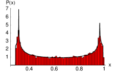
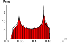
Figure 1: (Color online) Probability distributions for a small quench around a critical point. $P\left(x\right)=\overline{\delta\left(x-\mathcal{L}\left(t\right)\right)}$, $P\left(m\right)=\overline{\delta\left(m-\langle\sigma_{1}^{z}\left(t\right)\rangle\right)}$ refer to the Loschmidt echo (upper panel) and magnetization respectively (lower panel). The thick lines are obtained using the prediction of Eq. (7) using only the three largest weights. Note the large spread of the distributions compared with their total support: $P\left(x\right)\in\left[0,1\right]$ and $P\left(m\right)\in\left[-1,1\right]$. Parameters $L=16,\,\kappa_{1}=\kappa_{2}=0.4,\,h_{1}=0.218$, $\delta h=h_{2}-h_{1}=0.04$, are close to criticality (see Beccaria et al. (2006)). The data are obtained by Lanczos diagonalization of Eq. (8) keeping as many lowest energy vectors until the sum rule $\sum_{n=0}^{n_{\mathrm{max}}-1}p_{n}\simeq 1$ was satisfied within prescribed accuracy.

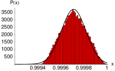
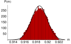
Figure 2: (Color online) Probability distributions for a small quench around a regular point. $P\left(x\right)=\overline{\delta\left(x-\mathcal{L}\left(t\right)\right)}$, $P\left(m\right)=\overline{\delta\left(m-\langle\sigma_{1}^{z}\left(t\right)\rangle\right)}$ refer to the Loschmidt echo (upper panel) and magnetization respectively (lower panel). The thick lines are Gaussian with the same mean and standard deviation. The quench is performed in the paramagnetic phase, parameters are $L=12,\,\kappa_{1}=\kappa_{2}=0.3,\,h_{1}=1.4$, $\delta h=0.04$. Note the very small spread of the distributions. The data are obtained by full diagonalization of the Hamiltonian Eq. (8). Histograms are obtained by sampling 40000 random times in an interval $t\in\left[0,T\right]$ with $T=16000$.

Numerical test

We will now check our predictions on the hand of a non-integrable model. As a test model we chose to use the so called TAM Hamiltonian (transverse axial next-nearest-neighbor Ising model). The Hamiltonian is

$$H=-\sum_{i=1}^{L}\left(\sigma_{i}^{x}\sigma_{i+1}^{x}-\kappa\sigma_{i}^{x}\sigma_{i+2}^{x}+h\sigma_{i}^{z}\right),$$ (8)

and periodic boundary conditions are used ($\sigma_{L+i}^{x}=\sigma_{i}^{x}$). A positive $\kappa$ frustrates the order in the $\sigma^{x}$ direction. The reason for our choice is, at least, twofold: i) The TAM is a non-integrable generalization of the one-dimensional quantum Ising model for which results are already available Campos Venuti and Zanardi (2009). ii) The model Eq. (8) has only a discrete $\mathbb{Z}_{2}$ symmetry ($P_{z}=\prod_{i}\sigma_{i}^{z}$), consequently the ground state lives in a large $d_{GS}=2^{L-1}$ dimensional space. In practice $d_{GS}$ is the effective Hilbert space dimension, and we would like it to be as large as possible. For instance, after a quench the purity of the equilibrium state is bounded by $\mathrm{tr}\left(\overline{\rho}^{2}\right)\geq d_{GS}^{-1}$. This is to be contrasted with other models used in the literature with larger symmetry groups (i.e. $SU\left(2\right)$) for which the dimension of the block containing the ground state is still exponential in $L$ but considerably reduced with respect to to that of the full Hilbert space $2^{L}$.

The model Eq. (8) displays 4 phases (see for instance Peschel and Emery (1981); Allen et al. (2001); Beccaria et al. (2006, 2007) and references therein), ferromagnetic $++++$, antiphase $++--$, paramagnetic, and a floating phase with algebraically decaying spin correlations. In particular, for small frustration $\kappa\leq 1/2$, increasing the external field $h$ there is a transition from ferromagnetic to paramagnetic. This transition is believed to fall in the Ising universality class, and so the critical theory is described by a conformal field theory with central charge $c=1/2$ and $d=\zeta=\nu=1$. We performed our numerical simulation for the critical quench on this critical line.

We will illustrate our findings for two particular yet physically well motivated observables; the Loschmidt echo $\mathcal{L}\left(t\right)=\left|\langle\psi_{0}|e^{-itH_{2}}|\psi_{0}\rangle\right|^{2}$ and the transverse magnetization $m\left(t\right)=\langle\psi_{0}\left(t\right)|\sigma_{i}^{z}|\psi_{0}\left(t\right)\rangle$.

Since $d=\zeta=\nu=1$, according to Eq. (3), we expect a strong divergence at low energy: $p\left(E\right)\sim E^{-2}$. Consequently we expect very few $p_{n},\,n>0$ to have non-negligible weight, and so Eq. (7) to be a valid approximation. Indeed the results based on numerical diagonalization compare well with the prediction based on Eq. (7) (Fig. 1). Note the very large spread of the distributions compared to their total support: “poor equilibration”.

For comparison we performed similar numerical simulation for a small quench in a regular point of the phase diagram. As expected the resulting distribution functions are approximately Gaussian (Fig. 2). Note the very small variances of the distributions already for a relatively short size: “good equilibration”

Conclusions

In this paper we investigated the detailed structure of equilibration after a small quench, i.e. the system is initialized in the ground state of a given Hamiltonian $H_{1}$ and then let evolve with a slightly perturbed Hamiltonian $H_{2}=H_{1}+\delta\lambda V$. In the limit $\delta\lambda\to 0$ equilibration is trivial in that for all observables $P\left(o\right)=\overline{\delta\left(o-\langle O\left(t\right)\rangle\right)}^{t}=\delta\left(o-\langle O\rangle\right)$. However this limit is approached very differently depending on whether Hamiltonian $H_{1}$ is critical or not. For quenches around a regular point of the phase diagram the expected distribution for generic observables is a Gaussian one. Equilibration arises in the most standard fashion. Instead for small quenches around a critical point the situation is radically different. The distribution function for generic observables $P\left(o\right)$ tends to universal double-peaked function for relevant perturbations.

The key step to obtain these results is to characterize the overlaps $c_{n}=\langle n|\psi_{0}\rangle$ between the initial state $|\psi_{0}\rangle$ and quenched Hamiltonian eigenstates $|n\rangle$. We have shown that, at criticality, the function $c\left(E_{n}\right)=c_{n}$ ($E_{n}$ eigenenergy) decays very rapidly: $c\left(E\right)\sim E^{-1/\left(\zeta\nu\right)}$ and this in turns generically implies the observed double-peaked distributions. The analytical predictions have been checked numerically on the hand of a non-integrable extension of the quantum Ising model.

LCV acknowledges support from European project COQUIT under FET-Open grant number 2333747 and PZ from NSF grants PHY-803304, DMR-0804914.

References

- Reimann (2008) P. Reimann, Phys. Rev. Lett. 101, 190403 (2008).
- Linden et al. (2009) N. Linden, S. Popescu, A. J. Short, and A. Winter, Phys. Rev. E 79, 061103 (2009).
- Kinoshita et al. (2006) T. Kinoshita, T. Wegner, and D. S. Weiss, Nature 440, 900 (2006).
- Sadler et al. (2006) L. E. Sadler, J. M. Higbie, S. R. Leslie, M. Vengalattore, and D. M. Stamper-Kurn, Nature 443, 312 (2006).
- Weiler et al. (2008) C. N. Weiler, T. W. Neely, D. R. Scherer, A. S. Bradley, M. J. Davis, and B. P. Anderson, Nature 455, 948 (2008).
- Campos Venuti and Zanardi (2009) L. Campos Venuti and P. Zanardi, Phys. Rev. A (2009), arXiv:0907.0683.
- Zanardi and Paunković (2006) P. Zanardi and N. Paunković, Phys. Rev. E 74, 031123 (2006).
- Zanardi et al. (2007a) P. Zanardi, P. Giorda, and M. Cozzini, Phys. Rev. Lett. 99, 100603 (2007a).
- Zhou and Barjaktarevic (2008) H.-Q. Zhou and J. P. Barjaktarevic, J. Phys. A: Math. Theor. 41, 412001 (2008).
- Gu (2008) S.-J. Gu (2008), arXiv:0811.3127v1.
- Campos Venuti and Zanardi (2007) L. Campos Venuti and P. Zanardi, Phys. Rev. Lett. 99, 095701 (2007).
- Schwandt et al. (2009) D. Schwandt, F. Alet, and S. Capponi, 103, 170501 (2009).
- Barankov (2009) R. A. Barankov (2009), arXiv:0910.0255.
- Prosen (1998) T. Prosen, Phys. Rev. Lett. 80, 1808 (1998).
- Jalabert and Pastawski (2001) R. A. Jalabert and H. M. Pastawski, Phys. Rev. Lett. 86, 2490 (2001).
- Quan et al. (2006) H. T. Quan, Z. Song, X. F. Liu, P. Zanardi, and C. P. Sun, Phys. Rev. Lett. 96, 140604 (2006).
- Rossini et al. (2007a) D. Rossini, T. Calarco, V. Giovannetti, S. Montangero, and R. Fazio, J. Phys. A: Math. Theor. 40, 8033 (2007a).
- Rossini et al. (2007b) D. Rossini, T. Calarco, V. Giovannetti, S. Montangero, and R. Fazio, Phys. Rev. A 75, 032333 (2007b).
- Zanardi et al. (2007b) P. Zanardi, H. T. Quan, X. Wang, and C. P. Sun, Phys. Rev. A 75, 032109 (2007b).
- Silva (2008) A. Silva, Phys. Rev. Lett. 101, 120603 (2008).
- Beccaria et al. (2006) M. Beccaria, M. Campostrini, and A. Feo, Phys. Rev. B 73, 052402 (2006).
- Peschel and Emery (1981) I. Peschel and V. J. Emery, Z. Phys. B: Condens. Matter 43, 241 (1981).
- Allen et al. (2001) D. Allen et al., J. Phys. A 34, L305 (2001).
- Beccaria et al. (2007) M. Beccaria, M. Campostrini, and A. Feo, Phys. Rev. B 76, 094410 (2007).
- Cramer et al. (2008) M. Cramer, C. M. Dawson, Eisert, and T. J. Osborne, Phys. Rev. Lett. 100, 030602 (2008).