A Chebychev propagator with iterative time ordering for explicitly time-dependent Hamiltonians

Abstract

A propagation method for time-dependent Schrödinger equations with an explicitly time-dependent Hamiltonian is developed where time ordering is achieved iteratively. The explicit time-dependence of the time-dependent Schrödinger equation is rewritten as an inhomogeneous term. At each step of the iteration, the resulting inhomogeneous Schrödinger equation is solved with the Chebychev propagation scheme presented in J. Chem. Phys. 130, 124108 (2009). The iteratively time-ordering Chebychev propagator is shown to be robust, efficient and accurate and compares very favorably to all other available propagation schemes.

I Introduction

The dynamics of the interaction of matter with a strong radiation field is described by time-dependent Schrödinger equations (TDSEs) where the Hamiltonian is explicitly time-dependent. This description is at the core of the theory of harmonic generation,Corkum94 ; Corkum05 pump-probe spectroscopy,engel98 and coherent control.k67 ; ZhuJCP98 Typically, an atom or molecule couples to a laser pulse via a dipole transition,

$$\boldsymbol{\mathsf{\hat{H}}}(t)=\boldsymbol{\mathsf{\hat{H}}}_{0}+E(t)\boldsymbol{\mathsf{\hat{\mu}}}\,,$$ (1)

with $E(t)$ the time-dependent electromagnetic field, causing the explicit time-dependence of the Hamiltonian. Simulating these light-matter processes from first principles imposes a numerical challenge. Realistic simulations require efficient procedures with very high accuracy.

For example, in coherent control processes, interaction of quantum matter with laser light leads to constructive interference in some desired channel and destructive interference in all other channels. In time-domain coherent control such as pump-probe spectroscopy, wave packets created by radiation at an early time interfere with wave packets generated at a later time. This means that the relative phase between different partial wave packets has to be maintained for long time with high accuracy. As a result, numerical methods designed to simulate such phenomena have to be highly accurate, minimizing the errors in both amplitude and phase.

The difficulty of simulating explicitly time-dependent Hamiltonians, emerges from the fact that the commutator of the Hamiltonian with itself at different times does not vanish,magnus09

$$[\boldsymbol{\mathsf{\hat{H}}}(t_{1}),\boldsymbol{\mathsf{\hat{H}}}(t_{2})]_{-}\neq 0\,.$$ (2)

Formally, this effect is taken into account by time ordering such that the time evolution is given by

$$\boldsymbol{\mathsf{\hat{U}}}(T,0)=\mathcal{T}e^{-\frac{i}{\hbar}\int_{0}^{T}\boldsymbol{\mathsf{\hat{H}}}(t)\,dt}\,.$$ (3)

The effect of time ordering is to incorporate higher order commutators into the propagator $\boldsymbol{\mathsf{\hat{U}}}(T,0)$. For strong fields $E(t)$ and fast time-dependences the convergence with respect to ordering is slow. Methods to incorporate the second order Magnus termmagnus have been developed either in a low order polynomial expansionk79 ; k92 or as a split exponential.klaiber09

A quantum dynamical propagator that fully accounts for time ordering is given by the $(t,t^{\prime})$ method.Ronniettprime It is based on rewriting the Hamiltonian in an extended Hilbert space where an auxiliary coordinate, $t^{\prime}$, is added and terms such as $E(t^{\prime})\boldsymbol{\mathsf{\hat{\mu}}}$ are treated as a potential in this degree of freedom. The Hamiltonian thus looses its explicit dependence on time $t$, and can be propagated with one of the available highly accurate methods for solving the TDSE with time-independent Hamiltonian.RonnieReview88

Most of the vast literature on the interaction of matter with time-dependent fields in general bandrauk91 ; engel98 ; fisher04 ; bandrauk06 and on coherent control in particular k67 ; ohtsuki98 ; ohtsuki08 ; rabitz08 ; GollubPRA08 ignores the effect of time ordering. Popular approaches include Runge-Kutta schemes,magnus ; KilinJCP09 ; TremblayJCP04 the standard Chebychev propagator with very small time step,MyPRA04 and the split propagator.feit ; bandrauk91 ; GollubPRA08 Naively it is assumed that if the time step is small enough the calculation with an explicit time-dependent Hamiltonian can be made to converge. The difficulty is that this convergence is very slow – second order in the time step if the Hamiltonian is stationary in the time interval and third order if the second order Magnus approximation is used.k79 ; KormannJCP08 Additionally in many cases the error accumulates in phasek71 ; k92 so that common indicators of error such as deviation from unitarity are misleading.

In order to obtain high quality simulations of explicitly time dependent problems a new approach has to be developed. The ultimate $(t,t^{\prime})$ method cannot be used in practice since it becomes prohibitively expensive in realistic simulations. On the other hand we want to maintain the exponential convergence property of spectral decomposition such as the Chebychev propagator. The solution is an iterative implementation of the Chebychev propagator for inhomogeneous equations such that it can overcome the time ordering issue.

The paper is organized as follows. The formal solution to the problem is introduced in Section II: The TDSE for an explicitly time-dependent Hamiltonian is rewritten as an inhomogeneous TDSE. The inhomogeneity is calculated iteratively and converges in the limit of many iterations. At each step of the iteration, an inhomogenenous TDSE is solved by a Chebychev propagator which is based on a polynomial expansion of the inhomogeneous term.NdongJCP09 The resulting algorithm is outlined explicitly in Section III and applied to three different examples in Section IV. Its high accuracy is demonstrated and its efficiency is discussed in comparison to other approaches. Section V concludes.

II Formal solution

The Hamiltonian, $\boldsymbol{\mathsf{\hat{H}}}$, describing the interaction of a quantum system with a time-dependent external field typically consists of a field-free, time-independent part, $\boldsymbol{\mathsf{\hat{H}}}_{0}$, and an interaction term, $\boldsymbol{\mathsf{\hat{W}}}(t)=\boldsymbol{\mathsf{\hat{\mu}}}E(t)$. The TDSE for such a Hamiltonian (setting $\hbar=1$),

$$i\frac{\partial}{\partial t}|\psi(t)\rangle=\big{(}\boldsymbol{\mathsf{\hat{H}}}_{0}+\boldsymbol{\mathsf{\hat{W}}}(t)\big{)}|\psi(t)\rangle\,,$$ (4)

is solved numerically by dividing the overall propagation time $[0,T]$ into short time intervals $[t_{n},t_{n+1}]$, each of length $\Delta t$. A two-stage approach is employed. First, the formal solution of the TDSE is considered. The term arising from the explicit time-dependence of the Hamiltonian is approximated iteratively. The iterative loop thus takes care of the time ordering. Second, at each step of the iteration, an inhomogeneous Schrödinger equation is obtained. It is solved with the recently introduced Chebychev propagator for inhomogeneous Schrödinger equations.NdongJCP09

II.1 Iterative time ordering

The TDSE, Eq. (4), is rewritten to capture the time-dependence within the interval $[t_{n},t_{n+1}]$,

$$i\frac{\partial}{\partial t}|\psi(t)\rangle=\big{(}\boldsymbol{\mathsf{\hat{H}}}_{0}+\boldsymbol{\mathsf{\hat{W}}}_{n}\big{)}|\psi(t)\rangle\,+\,\big{(}\boldsymbol{\mathsf{\hat{W}}}(t)-\boldsymbol{\mathsf{\hat{W}}}_{n}\big{)}|\psi(t)\rangle\,.$$ (5)

Here, $\boldsymbol{\mathsf{\hat{W}}}_{n}$ is the value of $\boldsymbol{\mathsf{\hat{W}}}(t)$ at the midpoint of the propagation interval, $\boldsymbol{\mathsf{\hat{W}}}_{n}=\boldsymbol{\mathsf{\hat{W}}}\left(\frac{t_{n+1}+t_{n}}{2}\right)$. The formal solution of Eq. (5) is given by

$$|\psi(t)\rangle = e^{-i\boldsymbol{\mathsf{\hat{H}}}_{n}(t-t_{n})}|\psi(t_{n})\rangle-$$ (6)

$$i\int_{t_{n}}^{t}{e^{-i\boldsymbol{\mathsf{\hat{H}}}_{n}(t-\tau)}\boldsymbol{\mathsf{\hat{V}}}_{n}(\tau)|\psi(\tau)\rangle d\tau}\,,$$

where $\boldsymbol{\mathsf{\hat{H}}}_{n}=\boldsymbol{\mathsf{\hat{H}}}_{0}+\boldsymbol{\mathsf{\hat{W}}}_{n}$ denotes the part that is independent of time in $[t_{n},t_{n+1}]$ and $\boldsymbol{\mathsf{\hat{V}}}_{n}(t)=\boldsymbol{\mathsf{\hat{W}}}(t)-\boldsymbol{\mathsf{\hat{W}}}_{n}$ the time-dependent part. Eq. (6) is subjected to an iterative loop,

$$|\psi_{k}(t)\rangle = e^{-i\boldsymbol{\mathsf{\hat{H}}}_{n}(t-t_{n})}|\psi_{k}(t_{n})\rangle-$$ (7)

$$i\int_{t_{n}}^{t}{e^{-i\boldsymbol{\mathsf{\hat{H}}}_{n}(t-\tau)}\boldsymbol{\mathsf{\hat{V}}}_{n}(\tau)|\psi_{k-1}(\tau)\rangle d\tau}\,,$$

The solution at the $k$th step of the iteration, $|\psi_{k}\rangle$, is calculated from the formal solution, Eq. (6), by replacing $|\psi_{k}\rangle$ in the second term on the right-hand side of Eq. (6) by $|\psi_{k-1}\rangle$ which is known from the previous step.

In this approach, time ordering is achieved by converging $|\psi_{k-1}\rangle$ to $|\psi_{k}\rangle$ as the iterative scheme proceeds. This is equivalent to the derivation of the Dyson series. Starting from the equation of motion for the time evolution operator,

$$i\frac{\partial}{\partial t}\boldsymbol{\mathsf{\hat{U}}}(t,0)=\boldsymbol{\mathsf{\hat{H}}}(t)\boldsymbol{\mathsf{\hat{U}}}(t,0)\,,$$

the formal solution for the time evolution operator,

$$\boldsymbol{\mathsf{\hat{U}}}(t,0)=-i\int_{0}^{t}\boldsymbol{\mathsf{\hat{H}}}(t_{1})\boldsymbol{\mathsf{\hat{U}}}(t_{1},0)dt_{1}\,,$$ (8)

is iteratively inserted in the right-hand side, i.e.

$$\boldsymbol{\mathsf{\hat{U}}}(t,0) = -i\int_{0}^{t}\int_{0}^{t_{1}}\boldsymbol{\mathsf{\hat{H}}}(t_{1})\boldsymbol{\mathsf{\hat{H}}}(t_{2})\boldsymbol{\mathsf{\hat{U}}}(t_{2},0)dt_{2}dt_{1}\,,$$

$$\ldots$$

$$\boldsymbol{\mathsf{\hat{U}}}(t,0) = -i\int_{0}^{t}\int_{0}^{t_{1}}\ldots\int_{0}^{t_{n-1}}$$

$$\boldsymbol{\mathsf{\hat{H}}}(t_{1})\boldsymbol{\mathsf{\hat{H}}}(t_{2})\ldots\boldsymbol{\mathsf{\hat{H}}}(t_{n})\boldsymbol{\mathsf{\hat{U}}}(t_{n},0)dt_{n}\ldots dt_{2}dt_{1}\,,$$

where $\boldsymbol{\mathsf{\hat{U}}}(t_{n},0)$ goes to 11 as $t_{n}$ becomes smaller and smaller. Our formal solution, Eq. (6) is equivalent to Eq. (8). An alternative approach to time ordering is given by the Magnus expansion which is based on the group properties of unitary time evolution.magnus In the limit of convergence, the Magnus and the Dyson series are completely equivalent, but low-order approximations of the two differ.magnus Our iterative scheme corresponds to the limit of convergence (with respect to machine precision).

II.2 Equivalence to an inhomogeneous TDSE

Differentiating Eq. (7) with respect to time, an inhomogeneous Schrödinger equation at each step $k$ of the iteration is obtained,

$$\frac{\partial}{\partial t}|\psi_{k}(t)\rangle=-i\boldsymbol{\mathsf{\hat{H}}}_{n}|\psi_{k}(t)\rangle+|\Phi_{k-1}(t)\rangle\,.$$ (9)

The inhomogeneity is given by

$$|\Phi_{k-1}(t)\rangle=-i\boldsymbol{\mathsf{\hat{V}}}_{n}(t)|\psi_{k-1}(t)\rangle\,.$$ (10)

Eq. (9) can be solved by approximating the inhomogeneous term globally within $[t_{n},t_{n+1}]$, i.e. by expanding it into Chebychev polynomials,

$$|\Phi_{k-1}(t)\rangle\approx\sum_{j=0}^{m-1}P_{j}(\bar{t})|\bar{\Phi}_{k-1,j}\rangle\,.$$ (11)

$P_{k-1,j}$ denotes the Chebychev polynomial of order $j$ with expansion coefficient $|\bar{\Phi}_{k-1,j}\rangle$, and $\bar{t}=2(t-t_{n})/\Delta t-1$ with $t\in[t_{n},t_{n+1}]$ is a rescaled time.NdongJCP09

The expansion coefficients, $|\bar{\Phi}_{k-1,j}\rangle$, in Eq. (11) are given by

$$|\bar{\Phi}_{k-1,j}\rangle=\frac{2-\delta_{j0}}{\pi}\int_{-1}^{1}\frac{|\Phi_{k-1}(\bar{t})\rangle P_{j}(\bar{t})}{\sqrt{1-\bar{t}^{2}}}d\bar{t}\,.$$ (12)

Since $|\Phi_{k-1}(\bar{t})\rangle$ is known at each point in the interval and in particular at the zeros, $\bar{t}_{i}$, of the $m$th Chebychev polynomial, the integral in Eq. (12) can be rewritten by applying a Gaussian quadrature,RoiPRA00 yielding

$$|\bar{\Phi}_{k-1,j}\rangle=\frac{2-\delta_{j0}}{m}\sum_{i=0}^{m-1}|\Phi_{k-1}(\bar{t}_{i})\rangle P_{j}(\bar{t}_{i})\,.$$ (13)

Due to the fact that the Chebychev polynomials can be expressed in terms of cosines, Eq. (13) is equivalent to a cosine transformation. Thus the expansion coefficients, $|\bar{\Phi}_{k-1,j}\rangle$, can easily be obtained numerically by fast cosine transformation.

The expansion into Chebychev polynomials, if converged, is equivalent to the following alternative expansion,

$$\sum_{j=0}^{m-1}P_{j}(\bar{t})|\bar{\Phi}_{k-1,j}\rangle=\sum_{j^{\prime}=0}^{m-1}\frac{(t-t_{n})^{j^{\prime}}}{j^{\prime}!}|\Phi_{k-1}^{(j^{\prime})}\rangle\,.$$ (14)

Once the coefficients of the Chebychev expansion, $|\bar{\Phi}_{k-1,j}\rangle$, are known, the transformation described in Appendix A is used to generate the coefficients $|\Phi_{k-1}^{(j^{\prime})}\rangle$ in Eq. (14).

Approximating the inhomogeneous term by the right-hand side of Eq. (14), the formal solution of Eq. (9) can be writtenNdongJCP09

$$|\psi_{k}(t)\rangle=\sum_{j=0}^{m-1}\frac{(t-t_{n})^{j}}{j!}|\lambda^{(j)}_{k-1}\rangle+\boldsymbol{\mathsf{\hat{F}}}_{m}|\lambda^{(m)}_{k-1}\rangle\,,$$ (15)

where the $|\lambda^{(j)}_{k-1}\rangle$ are obtained recursively,

$$|\lambda^{(0)}_{k-1}\rangle = |\psi(t_{n})\rangle\,,$$ (16)

$$|\lambda^{(j)}_{k-1}\rangle = -i\boldsymbol{\mathsf{\hat{H}}}_{n}|\lambda^{(j-1)}_{k-1}\rangle+|\Phi^{(j-1)}_{k-1}\rangle,$$

$$\quad\quad 1\leq j\leq m\,.$$

$\boldsymbol{\mathsf{\hat{F}}}_{m}$ is a function of $\boldsymbol{\mathsf{\hat{H}}}_{n}$ and is given by

$$\boldsymbol{\mathsf{\hat{F}}}_{m} =$$

$$(-i\boldsymbol{\mathsf{\hat{H}}}_{n})^{-m}\left(e^{-i\boldsymbol{\mathsf{\hat{H}}}_{n}(t-t_{n})}-\sum_{j=0}^{m-1}\frac{(-i\boldsymbol{\mathsf{\hat{H}}}_{n}(t-t_{n}))^{j}}{j!}\right)\,.$$

Taking the derivative of Eq. (15) with respect to time, the inhomogeneous Schrödinger equation is recovered after some algebra.NdongJCP09

Alternatively, Eq. (10) can be inserted into Eq. (7), replacing $|\Phi_{k-1}\rangle$ by its polynomial approximation, Eq. (11),

$$|\psi(t)\rangle = e^{-i\boldsymbol{\mathsf{\hat{H}}}_{n}t}|\psi(0)\rangle+$$ (18)

$$e^{-i\boldsymbol{\mathsf{\hat{H}}}_{n}t}\sum_{j=0}^{m-1}\int_{0}^{t}{e^{i\boldsymbol{\mathsf{\hat{H}}}_{n}\tau}\frac{\tau^{j}}{j!}|\Phi^{(j)}\rangle d\tau}$$

(without any loss of generality, $t_{n}$ has been set to zero). Defining

$$\boldsymbol{\mathsf{\hat{\alpha}}}_{j}=e^{-i\boldsymbol{\mathsf{\hat{H}}}_{n}t}\int_{0}^{t}{e^{i\boldsymbol{\mathsf{\hat{H}}}_{n}\tau}\frac{\tau^{j}}{j!}d\tau}\,,$$ (19)

and integrating Eq. (19) by parts, one obtains

$$\boldsymbol{\mathsf{\hat{\alpha}}}_{j} = (-i\boldsymbol{\mathsf{\hat{H}}}_{n})^{-1}\left(e^{-i\boldsymbol{\mathsf{\hat{H}}}_{n}t}\boldsymbol{\mathsf{\hat{\alpha}}}_{j-1}-\frac{t^{j}}{j!}\leavevmode\hbox{\small 1\kern-3.3pt\normalsize 1}\right)\,,$$

$$\quad 1\leq j\leq m-1\,,$$

$$\boldsymbol{\mathsf{\hat{\alpha}}}_{0} = (-i\boldsymbol{\mathsf{\hat{H}}}_{n})^{-1}\left(e^{-i\boldsymbol{\mathsf{\hat{H}}}_{n}t}-\leavevmode\hbox{\small 1\kern-3.3pt\normalsize 1}\right)\,.$$ (21)

By induction, it follows that

$$\boldsymbol{\mathsf{\hat{\alpha}}}_{j}=(-i\boldsymbol{\mathsf{\hat{H}}}_{n})^{-(j+1)}\left(e^{-i\boldsymbol{\mathsf{\hat{H}}}_{n}t}-\sum_{a=0}^{j}\frac{(-i\boldsymbol{\mathsf{\hat{H}}}_{n}t)^{a}}{a!}\right)\,.$$ (22)

Defining

$$\boldsymbol{\mathsf{\hat{F}}}_{j+1}=(-i\boldsymbol{\mathsf{\hat{H}}}_{n})^{-(j+1)}\left(e^{-i\boldsymbol{\mathsf{\hat{H}}}_{n}t}-\sum_{a=0}^{j}\frac{(-i\boldsymbol{\mathsf{\hat{H}}}_{n}t)^{a}}{a!}\right)\,,$$ (23)

Eq. (18) becomes

$$|\psi(t)\rangle=e^{-i\boldsymbol{\mathsf{\hat{H}}}_{n}t}|\psi(0)\rangle+\sum_{j=0}^{m-1}\boldsymbol{\mathsf{\hat{F}}}_{j+1}|\Phi^{(j)}\rangle\,,$$ (24)

which was shown to be equivalent to Eq. (15).NdongJCP09

The algorithm for solving the TDSE with explicitly time-dependent Hamiltonian is thus based on evaluating the integral of the formal solution, Eq. (6), in an iterative fashion. At each step $k$ of the iteration, the inhomogeneous TDSE, Eq. (9), is solved by applying the propagator of Ref. NdongJCP09, within each short time interval $[t_{n},t_{n+1}]$.

Once convergence with respect to the iteration $k$ is reached, the inhomogeneous term becomes constant with respect to $k$.

III Outline of the algorithm

We assume that the action of the Hamiltonian on a wavefunction can be efficiently computed.RonnieReview88 Then the complete propagation time interval $[0,T]$ is split into small time intervals, $[t_{n},t_{n+1}]$. For each time step $[t_{n},t_{n+1}]$, the implementation of the Chebychev propagator with iterative time ordering involves an outer loop over the iterative steps $k$ for time ordering and an inner loop over $j$ for the solution of the (inhomogeneous) Schrödinger equation for each $k$.

1. Preparation: Set a local time grid $\{\tau_{l}\}$ for each short-time interval $[t_{n},t_{n+1}]$. In order to calculate the expansion coefficients of the inhomogeneous term by cosine transformation, the $N_{t}$ sampling points $\{\tau_{l}\}$ are chosen to be the roots of the Chebychev polynomial $P_{N_{t}}$ of order $N_{t}$. The number of sampling points, $N_{t}$, is not known in advance. One thus has to provide an initial guess and check below, in step 3.i, that it is equal to or larger than the number of Chebychev polynomials required to expand the inhomogeneous term,

   $$N_{t}\geq m\,.$$ (25)

   If $N_{t}$ is much larger than $m$, it is worth to decrease it (subject to the bound of Eq. (25)) and to recalculate the $\{\tau_{l}\}$. The number of propagation steps within $[t_{n},t_{n+1}]$ is then reduced to its mininum.

2. The propagation for $k=0$ solves the Schrödinger equation for the time-independent Hamiltonian $\boldsymbol{\mathsf{\hat{H}}}_{n}=\boldsymbol{\mathsf{\hat{H}}}_{0}+\boldsymbol{\mathsf{\hat{W}}}_{n}$,

   $$i\frac{\partial}{\partial\tau}|\psi_{0}(\tau)\rangle=\big{(}\boldsymbol{\mathsf{\hat{H}}}_{0}+\boldsymbol{\mathsf{\hat{W}}}_{n}\big{)}|\psi_{0}(\tau)\rangle\,,$$

   with initial condition $|\psi_{0}(t=t_{n})\rangle=|\psi(t_{n})\rangle$. A standard Chebychev propagator is employed to this end. Note that for $k=0$, the same time grid $\{\tau_{l}\}$ needs to be used as for $k>0$ because the inhomogeneous term for $k=1$ is calculated from the zeroth order solution, $|\psi_{0}(t)\rangle$. Since the $\{\tau_{l}\}$ are not equidistant, the Chebychev expansion coefficients of the standard propagator, $e^{-i\boldsymbol{\mathsf{\hat{H}}}_{n}\Delta\tau_{l}}$, need to be calculated for each time step within $[t_{n},t_{n+1}]$, where $\Delta\tau_{l}=\tau_{l+1}-\tau_{l}$, $l=1,N_{t}-1$.

3. The $k>0$ propagation solves an inhomogeneous Schrödinger equation, cf. Eq. (9), with the initial condition $|\psi_{k}(t=t_{n})\rangle=|\psi_{0}(t=t_{n})\rangle=|\psi(t_{n})\rangle$. This is achieved by the Chebychev propagator for inhomogeneous Schrödinger equations,NdongJCP09 i.e. Eq. (15), and involves the following steps:

   1. Evaluate the inhomogeneous term, $|\Phi_{k-1}(\tau)\rangle=-i\big{(}\boldsymbol{\mathsf{\hat{W}}}(\tau)-\boldsymbol{\mathsf{\hat{W}}}_{n}\big{)}|\psi_{k-1}(\tau)\rangle$.

   2. Calculate the expansion coefficients of the inhomogeneous term, cf. Eqs. (11) and (14). The Chebychev expansion coefficients $|\bar{\Phi}_{k-1,j}\rangle$ are obtained by cosine transformation of $|\Phi_{k-1}(\tau)\rangle$.NdongJCP09 The coefficients $|\Phi^{(j)}_{k-1}\rangle$ are evaluated from the Chebychev expansion coefficients $|\bar{\Phi}_{k-1,j}\rangle$ using the recursive relation given in Eqs. (52) and (53). The order $m$ of the expansion is chosen such that ratio of the smallest to the largest Chebychev coefficient becomes smaller than the specified error $\epsilon$,

      $$\frac{\|\bar{\Phi}_{k-1,m+1}\|}{\|\bar{\Phi}_{k-1,0}\|}<\epsilon\,.$$ (26)

      To obtain high accuracy, $\epsilon$ may correspond to the machine precision.

   3. Calculate the Chebychev expansion coefficients of $\boldsymbol{\mathsf{\hat{F}}}_{m}$, cf. Eq. (II.2), also by cosine transformation. The number of terms in this Chebychev expansion is also determined by the relative magnitude of the coefficients, analogously to Eq. (26).

   4. Determine all $|\lambda^{(j)}_{k-1}\rangle$ required in Eq. (15) by evaluating Eq. (16).

   5. Construct the solution $|\psi_{k}(t=t_{n+1})\rangle$ according to Eq. (15).

4. Convergence is reached when $|\psi_{k-1}(t_{n+1})\rangle$ and $|\psi_{k}(t_{n+1})\rangle$ become indistinguishable,

   $$\|\psi^{k-1}(t_{n+1})-|\psi^{k}(t_{n+1})\|<\epsilon\,,$$

   and the desired solution of the Schrödinger equation with explicitly time-dependent Hamiltonian is obtained, $|\psi(t_{n+1})\rangle=|\psi_{k}(t_{n+1})\rangle$.

The only parameter of the algorithm is the pre-specified error $\epsilon$. It determines the number of iterative terms $k$ and the order of the inhomogeneous propagator $m$. Furthermore, to execute the algorithm, the user has to provide, besides $\epsilon$, an initial guess for the number of sampling points of the local time grid, $N_{t}$.

IV Examples

We test the accuracy and efficiency of the algorithm for three examples of increasing complexity. The first two examples, a driven two-level atom and a linearly driven harmonic oscillator, are analytically solvable. We can therefore compare the numerical to the analytical solution and establish the accuracy of the Chebychev propagator with iterative time ordering. For the third example, wave packet interferometry in two oscillators coupled by a field, no analytical solution is known. The Chebychev propagator with iterative time ordering thus serves as a reference solution to which less accurate methods can be compared.

IV.1 Driven two-level atom

The Hamiltonian for a two-level atom driven resonantly by a laser field in the rotating-wave approximation readsAllenEberly

$$\boldsymbol{\mathsf{\hat{H}}}=\begin{pmatrix}0&\boldsymbol{\mathsf{\hat{\mu}}}E(t)\\ \boldsymbol{\mathsf{\hat{\mu}}}E(t)&0\\ \end{pmatrix}\,,$$ (27)

where the field is of the form

$$E(t)=\frac{1}{2}E_{0}S(t)\,,$$ (28)

and $S(t)$ denotes the envelope of the field. We take the strength of the transition dipole to be $\mu=1\,$a.u., the final propagation time $T=9000\,$a.u., and the shape function

$$S(t)=\sin^{2}\left(\frac{\pi t}{T}\right)\,.$$ (29)

Analytically, the time evolution of the amplitudes,

$$|\psi(t)\rangle=\begin{pmatrix}c_{g}(t)\\ c_{e}(t)\end{pmatrix}\,,$$ (30)

is obtained as

$$c_{g}^{\mathrm{ana}}(t) = \cos\left[\frac{1}{4}\mu E_{0}\left(t-\frac{T}{2\pi}\sin\left(\frac{2\pi t}{T}\right)\right)\right]\,,$$ (31)

$$c_{e}^{\mathrm{ana}}(t) = i\sin\left[\frac{1}{4}\mu E_{0}\left(t-\frac{T}{2\pi}\sin\left(\frac{2\pi t}{T}\right)\right)\right]\,.$$ (32)

Initially the two-level system is assumed to be in the ground state, $c_{g}(t=0)=1$, $c_{e}(t=0)=0$. The pulse amplitude is chosen to yield a $\pi$-pulse, such that $c_{g}^{\mathrm{ana}}(t=T)=0$, $c_{e}^{\mathrm{ana}}(t=T)=1$.

Defining at each time step the errors,

$$\mathrm{\varepsilon_{sol}}(t)=\left||c_{g}^{\mathrm{ana}}(t)|^{2}-|c_{g}(t)|^{2}\right|\,,$$ (33)

and

$$\mathrm{\varepsilon_{norm}}(t)=\big{|}1-\langle\psi(t)|\psi(t)\rangle\big{|}\,,$$ (34)

we measure the deviation of the numerical from the analytical solution and the deviation of the norm of $|\psi(t)\rangle$ from unity. The time evolution of $\mathrm{\varepsilon_{sol}}(t)$ and $\mathrm{\varepsilon_{norm}}(t)$ is shown in Fig. 1 for the Chebychev propagator with iterative time ordering.

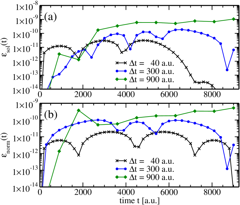
Figure 1: (color online) Strongly driven two-level atom propagated with iteratively time ordering Chebychev propagator: error of the solution, $\varepsilon_{\mathrm{sol}}(t)$ (a) and deviation of the norm of $|\psi(t)\rangle$ from unity, $\varepsilon_{\mathrm{norm}}(t)$ (b).

The maximum errors occuring during the propagation, $\mathrm{\varepsilon_{norm}^{\max}}$ and $\mathrm{\varepsilon_{sol}^{\max}}$, are also summarized in Table 1.

$\Delta t$	$N_{t}$	$m_{k}$	$N_{\mathrm{Cheby}}$	$\mathrm{\varepsilon_{sol}^{\max}}$	$\mathrm{\varepsilon_{norm}^{\max}}$	CPU time	$k_{\max}$
10	6	$4\,$	10	$1.7\cdot 10^{-11}$	$1.1\cdot 10^{-11}$	$23\,$s	3
	12	$4\,$	10	$1.7\cdot 10^{-11}$	$1.1\cdot 10^{-11}$	$47\,$s	3
20	7	$5\,$	11	$4.1\cdot 10^{-11}$	$1.8\cdot 10^{-11}$	$14\,$s	4
	14	$5\,$	11	$4.1\cdot 10^{-11}$	$1.8\cdot 10^{-11}$	$29\,$s	4
40	7	$5\,$	14	$3.1\cdot 10^{-11}$	$1.2\cdot 10^{-11}$	$8\,$s	4
	14	$5\,$	14	$3.1\cdot 10^{-11}$	$1.2\cdot 10^{-11}$	$15\,$s	4
80	8	6	16	$1.9\cdot 10^{-11}$	$1.1\cdot 10^{-11}$	$6\,$s	5
	16	6	16	$1.9\cdot 10^{-11}$	$1.1\cdot 10^{-11}$	$11\,$s	5
100	9	7	17	$8.3\cdot 10^{-11}$	$4.0\cdot 10^{-11}$	$5\,$s	5
	18	7	17	$8.3\cdot 10^{-11}$	$4.0\cdot 10^{-11}$	$9\,$s	5
300	10	8	29	$1.9\cdot 10^{-10}$	$1.0\cdot 10^{-10}$	$3.4\,$s	6
	20	9	29	$1.9\cdot 10^{-10}$	$1.0\cdot 10^{-10}$	$5.3\,$s	6
600	12	10	32	$5.7\cdot 10^{-10}$	$3.1\cdot 10^{-10}$	$2.6\,$s	6
	24	10	32	$5.7\cdot 10^{-10}$	$3.1\cdot 10^{-10}$	$4.2\,$s	6
700	12	10	33	$7.8\cdot 10^{-10}$	$3.6\cdot 10^{-10}$	$2.1\,$s	7
	24	10	33	$7.8\cdot 10^{-10}$	$3.6\cdot 10^{-10}$	$3.8\,$s	7
800	14	12	35	$5.2\cdot 10^{-10}$	$2.3\cdot 10^{-10}$	$2.5\,$s	8
	28	12	35	$5.2\cdot 10^{-10}$	$2.3\cdot 10^{-10}$	$4.3\,$s	8
900	15	13	36	$1.1\cdot 10^{-9}$	$5.3\cdot 10^{-10}$	$3.0\,$s	8
	30	13	36	$1.1\cdot 10^{-9}$	$5.3\cdot 10^{-10}$	$5.1\,$s	8
1000	17	15	38	$3.6\cdot 10^{-9}$	$7.0\cdot 10^{-10}$	$3.5\,$s	9
	34	15	38	$3.6\cdot 10^{-9}$	$7.0\cdot 10^{-10}$	$5.8\,$s	9

Table 1: The maximum error of the solution, $\mathrm{\varepsilon_{sol}^{\max}}$, and the maximum deviation of the norm from unity, $\mathrm{\varepsilon_{norm}^{\max}}$, occuring in the overall propagation time are listed together with the required CPU time for several short time intervals $\Delta t$. $N_{t}$ denotes the number of sampling points within $\Delta t$, $N_{\mathrm{Cheby}}$ the largest number of Chebychev coefficients in the expansion of $\boldsymbol{\mathsf{\hat{F}}}_{m}$, $m_{k}$ the order of the expansion of the inhomogeneous term and $k_{\max}$ the largest number of the iterations for time ordering occuring for all time intervals $[t_{n},t_{n+1}]$.

For time steps, $\Delta t=t_{n+1}-t_{n}$, up to about $T/100$, the maximum errors occuring during the propagation, $\mathrm{\varepsilon_{sol}^{\max}}$, are of the order of $10^{-11}$. If the time step is further increased to about $T/10$, the maximum errors are of the order of $10^{-9}$. The increase in $\mathrm{\varepsilon_{sol}^{\max}}$ is accompanied by an increase in $\mathrm{\varepsilon_{norm}^{\max}}$ as the time steps become larger, cf. Table 1. The deviation from unitarity indicates that the error is due to the Chebychev expansion of the time evolution which becomes unitary only once the series is converged. The limiting factor here is the accuracy of the numerically obtained Chebychev expansion coefficients. This effect becomes more severe, as the argument of the Chebychev polynomials, $\Delta t\Delta E$ (and thus the largest expansion coefficient) becomes larger and larger.

The errors obtained by the Chebychev propagator with iterative time ordering of the order of $10^{-11}$ to $10^{-9}$ have to be compared to those obtained by the standard Chebychev propagator, i.e. neglecting all effects due to time ordering. The latter yields maximum solution errors, $\mathrm{\varepsilon_{sol}^{\max}}$, of the order of $10^{-4}$ for $\Delta t=10\,$a.u.$=T/900$ and $10^{-3}$ for $\Delta t=40\,$a.u. The smallest $\mathrm{\varepsilon_{sol}^{\max}}$ that can be achieved without time ordering is of the order of $10^{-6}$ for $\Delta t=10^{-2}\,$a.u.$=T/900000$. Thus the numerical results obtained with the iterative method are highly accurate compared to those obtained by the standard Chebychev propagator neglecting time ordering.

Regarding the numerical efficiency of the Chebychev propagator with iterative time ordering, several conclusions can be drawn from Table 1. First of all, it is absolutely sufficient to choose the number of sampling points within the interval $\Delta t$, $N_{t}$, only slightly larger than the order of the expansion of the inhomogeneous term, $m_{k}$. Doubling $N_{t}$ doesn’t yield better accuracy but requires more CPU time. Second, we expect an optimum in terms of CPU time as $\Delta t$ is increased. A Chebychev expansion always comes with an offset and becomes more efficient as more terms in the expansion but less time steps are required (this concerns both Chebychev expansions, that for the inhomogeneous term of order $m_{k}$ and that for the time evolution operator, i.e. for the $\boldsymbol{\mathsf{\hat{F}}}_{m}$, of order $N_{\mathrm{Cheby}}$). However, this trend is countered by a higher number of iterations for time ordering, $k_{\mathrm{max}}$. According to Table 1, the optimum in terms of CPU time is found for $\Delta t\approx 700\,$a.u. Finally, the order required in the Chebychev expansion of the inhomogeneous term, $m_{k}$, stays comparatively small, well below the values where the transformation between the Chebychev coefficients and the polynomial coefficients becomes numerically instable, cf. Appendix A.

IV.2 Driven harmonic oscillator

As a second example, we consider a harmonic oscillator of mass $m=1\,$a.u. and frequency $\omega=1\,$a.u. driven by a linearly polarized field. The time-dependent Hamiltonian is given by

$$\boldsymbol{\mathsf{\hat{H}}}(r;t)=-\frac{1}{2}\frac{\partial^{2}}{\partial r^{2}}+\frac{1}{2}r^{2}+rE_{0}S(t)\cos(\omega_{0}t)\,,$$ (35)

where $E_{0}$ is the maximum field amplitude, $S(t)$ the shape function given by Eq. (29), and $\omega_{0}$ is the frequency of the driving field. The final time is set to $T=100\,$a.u. The Hamiltonian is represented on a Fourier gridRonnieReview88 with $N_{\mathrm{grid}}=128$ grid points, and $r_{\mathrm{max}}=10\,$a.u.$=-r_{\mathrm{min}}$. The transition probabilities and expectation values of position and momentum as a function of time are known analytically.Ronniettprime ; SalaminJPM95

Taking the initial wave function $|\psi(t=0)\rangle$ to be the ground state of the harmonic oscillator, we again measure the deviation of the numerical from the analytical solution, $\mathrm{\varepsilon_{sol}}$, and the deviation of the norm of $|\psi(t)\rangle$ from unity, $\mathrm{\varepsilon_{norm}}$, for the time-dependent probability of the oscillator to be in the ground state. The pulse amplitude is chosen to completely deplete the population of the ground state.

Two cases are analyzed which both correspond to strong resonant driving of the oscillator. In the first case the rotating-wave approximation is invoked, i.e. we set $\omega_{0}=0$. This eliminates the highly oscillatory term from the field, keeping only the time-dependence of the shape function (moderate time-dependence). In the second case, the rotating-wave approximation is avoided, $\omega_{0}=\omega$, i.e. the time-dependence of the Hamiltonian is much stronger than in the first case (strong time-dependence).

In order to compare the Chebychev propagators with and without time ordering, we first list the smallest $\mathrm{\varepsilon_{sol}^{\max}}$ and $\mathrm{\varepsilon_{norm}^{\max}}$ achieved by the standard Chebychev propagator without time ordering in Table 2.

$\Delta t$	$N_{\mathrm{Cheby}}$	$\mathrm{\varepsilon_{norm}^{\max}}$ ($\omega_{0}=\omega$)	$\mathrm{\varepsilon_{norm}^{\max}}$ ($\omega_{0}=0$)	$\mathrm{\varepsilon_{sol}^{\max}}$ ( $\omega_{0}=\omega$)	$\mathrm{\varepsilon_{sol}^{\max}}$ ($\omega_{0}=0$)	CPU time
$10^{-6}\,$a.u.	4	$6.8\cdot 10^{-9}$	$6.7\cdot 10^{-9}$	$4.6\cdot 10^{-8}$	$6.7\cdot 10^{-9}$	$1\,$ h $16\,$ m $28\,$s
$10^{-5}\,$a.u.	5	$6.6\cdot 10^{-10}$	$6.6\cdot 10^{-10}$	$4.7\cdot 10^{-7}$	$4.4\cdot 10^{-9}$	$9\,$ m $26\,$s
$10^{-4}\,$a.u.	7	$1.3\cdot 10^{-11}$	$4.7\cdot 10^{-11}$	$4.7\cdot 10^{-6}$	$4.2\cdot 10^{-8}$	$1\,$ m $28\,$s
$10^{-3}\,$a.u.	10	$6.5\cdot 10^{-12}$	$7.3\cdot 10^{-12}$	$4.7\cdot 10^{-5}$	$4.2\cdot 10^{-7}$	$12\,$s

Table 2: Driven harmonic oscillator with ($\omega_{0}=0$) and without ($\omega_{0}=\omega$) the rotating-wave approximation for the standard Chebychev propagator without time ordering. $N_{\mathrm{Cheby}}$ is the number of Chebychev polynomials required for the expansion of $e^{-i\boldsymbol{\mathsf{\hat{H}}}\Delta t}$.

The standard Chebychev propagator was developed for time-independent problems and is most efficient for large time steps. Here, however, extremely small time steps $\Delta t$ have to be employed to minimize the error due to the time-dependence of the Hamiltonian. Consequently, the required CPU times become quickly very large. Note that the deviation of the norm from unity is much smaller than the error of the solution. This means that norm conservation cannot serve as an indicator for the error due to the time-dependence of the Hamiltonian. This error is clearly non-negligible even for the very small time steps shown in Table 2.

Tables 3 and 4 compare the results for the driven harmonic oscillator obtained by the Chebychev propagator with iterative time ordering (ITO) and without time ordering (standard Chebychev propagator). The rotating-wave approximation is invoked in Table 3, $\omega_{0}=0$, and avoided in Table 4, $\omega_{0}=\omega$.

with iterative time ordering (ITO)

without time ordering (standard)

$\Delta t$

$N_{t}$

$m_{k}$

$N_{\mathrm{Cheby}}$

$\mathrm{\varepsilon_{norm}^{\max}}$

$\mathrm{\varepsilon_{sol}^{\max}}$

CPU time

$k_{\max}$

$\Delta t$

$N_{\mathrm{Cheby}}$

$\mathrm{\varepsilon_{norm}^{\max}}$

$\mathrm{\varepsilon_{sol}^{\max}}$

CPU time

0.01 a.u.

10

$8\,$

9

$5.3\cdot 10^{-13}$

$5.3\cdot 10^{-13}$

$1\,$ m $54\,$s

2

0.01 a.u.

18

$1.4\cdot 10^{-12}$

$4.2\cdot 10^{-6}$

$2\,$s

0.02 a.u.

10

$8\,$

10

$1.4\cdot 10^{-13}$

$1.4\cdot 10^{-13}$

$58\,$s

2

0.02 a.u.

18

$5.7\cdot 10^{-12}$

$8.5\cdot 10^{-6}$

$1.28\,$s

0.04 a.u.

10

$8\,$

15

$5.5\cdot 10^{-13}$

$4.5\cdot 10^{-13}$

$31\,$s

2

0.04 a.u.

29

$6.15\cdot 10^{-12}$

$1.7\cdot 10^{-5}$

$1\,$s

0.1 a.u.

10

$8\,$

24

$1.4\cdot 10^{-12}$

$1.4\cdot 10^{-12}$

$27\,$s

3

0.1 a.u.

44

$1.5\cdot 10^{-12}$

$4.2\cdot 10^{-5}$

$0.52\,$s

Table 3: Comparison of the Chebychev propagator with iterative (ITO) and without time ordering for the driven harmonic oscillator in the rotating-wave approximation ($\omega_{0}=0$). Notation as in Table 1.

with iterative time ordering (ITO)

without time ordering (standard)

$\Delta t$

$N_{t}$

$m_{k}$

$N_{\mathrm{Cheby}}$

$\mathrm{\varepsilon_{sol}^{\max}}$

$\mathrm{\varepsilon_{norm}^{\max}}$

CPU time

$k_{\max}$

$\Delta t$

$N_{\mathrm{Cheby}}$

$\mathrm{\varepsilon_{norm}^{\max}}$

$\mathrm{\varepsilon_{sol}^{\max}}$

CPU time

0.01 a.u.

10

$8\,$

9

$8.2\cdot 10^{-14}$

$3.5\cdot 10^{-13}$

$2\,$ m $5\,$s

3

0.01 a.u.

18

$1.5\cdot 10^{-12}$

$4.6\cdot 10^{-4}$

$2\,$s

0.02 a.u.

10

$8\,$

10

$2.5\cdot 10^{-13}$

$3.6\cdot 10^{-12}$

$1\,$ m $34\,$s

3

0.02 a.u.

23

$4.7\cdot 10^{-12}$

$9.3\cdot 10^{-4}$

$1.28\,$s

0.04 a.u.

10

$8\,$

15

$3.6\cdot 10^{-13}$

$5.5\cdot 10^{-11}$

$56\,$s

3

0.04 a.u.

29

$8.9\cdot 10^{-12}$

$1.8\cdot 10^{-3}$

$1\,$s

Table 4: Comparison of the Chebychev propagator with iterative (ITO) and without time ordering for the driven harmonic oscillator without the rotating-wave approximation ($\omega_{0}=\omega$). Notation as in Table 1.

In the case of the rotating-wave approximation, both propagators conserve the norm on the order of $10^{-12}$. However, only the propagator with iterative time ordering achieves an accuracy of the solution of the same order of magnitude while the standard propagator yields errors of the order of $10^{-6}$ for the time steps listed in Table 3. The smallest maximum error of the solution achieved by the standard Chebychev propagator for $\omega_{0}=0$ is of the order of $10^{-8}$ for a norm deviation of the order of $10^{-11}$, cf. Tab. 2. However, this requires a prohibitively small time step, $\Delta t=10^{-4}$ a.u.

Even for a very strongly time-dependent Hamiltonian, when the rotating-wave approximation is not invoked ($\omega_{0}=\omega$), the Chebychev propagator with iterative time ordering yields similarly accurate results, with errors of the order of $10^{-13}$, cf. Table 4. For comparison, the error obtained for the standard Chebychev propagator without time ordering is of the order of $10^{-3}$ for the time steps reported in Table 4. The smallest errors achieved with the standard Chebychev propagator are of the order of $10^{-6}$ for a norm deviation of the order of $10^{-11}$ for extremely small time steps, cf. Table 2.

The error of the solution, $\mathrm{\varepsilon_{sol}}(t)$, is shown in Fig. 2 as a function of time for different time steps and a very strongly time-dependent Hamiltonian, $\omega_{0}=\omega$.

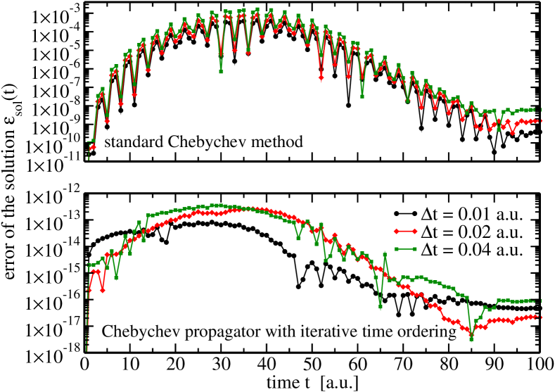
Figure 2: (color online) Strongly time-dependent Hamiltonian ($\omega_{0}=\omega$): Comparison of the Chebychev propagators without time ordering (standard) and with iterative time ordering in terms of the difference between the numerical and analytical solution, $\mathrm{\varepsilon_{sol}(t)}$.

This illustrates the superiority of the Chebychev propagator with iterative time ordering in terms of accuracy. A comparison of Tables 2 and 4 reveals furthermore that the Chebychev propagator with iterative time ordering is also more efficient than a standard Chebychev propagator with very small time step if a high accuracy of the solution is desired.

Since we have established the Chebychev propagator with iterative time ordering as a highly accurate method for the solution of the TDSE with explicitly time-dependent Hamiltonian, it is worthwhile to compare it to alternative propagation methods for this class of problems. In the following we will consider the $(t,t^{\prime})$ methodRonniettprime and a fourth-order Runge-Kutta scheme. The $(t,t^{\prime})$ method provides a numerically exact propagation scheme by translating the problem of time ordering into an additional degree of freedom of a time-independent Hamiltonian.Ronniettprime The TDSE for the Hamiltonian in the extended space is solved by numerically exact propagation schemes such as the Chebychev or Newton propagators.RonnieReview94 The $(t,t^{\prime})$ method is, however, relatively rarely used in the literature due to its numerical costs in terms of both CPU time and required storage. On the other hand, Runge-Kutta schemes are extremely popular in the literature.UlrichBenchmark00 They are potentially very accurate if a high-order variant is employed. Note that high order of a Runge-Kutta method implies evaluation of the Hamiltonian at several points within the time step $[t_{n},t_{n+1}]$.

In order to achieve a fair comparison between the Chebychev propagator with iterative time ordering and the $(t,t^{\prime})$ method, first the parameters which yield an optimal performance of the $(t,t^{\prime})$ method for our example have to be determined. The required CPU time and the errors, $\mathrm{\varepsilon_{sol}^{\max}}$ and $\mathrm{\varepsilon_{norm}^{\max}}$, as a function of the number of grid points, $N_{t^{\prime}}$ and $N_{t}$, are listed in Table 5.

$N_{t^{\prime}}$	$N_{t}$	$N_{\mathrm{Cheby}}$	$\mathrm{\varepsilon_{sol}^{\max}}$	$\mathrm{\varepsilon_{norm}^{\max}}$	CPU time
1024	1024	43	$2.3\cdot 10^{-12}$	$1.2\cdot 10^{-12}$	$16\,$ m $37\,$s
128	128	150	$3.0\cdot 10^{-13}$	$1.3\cdot 10^{-13}$	$43\,$s
128	16	906	$3.4\cdot 10^{-13}$	$1.7\cdot 10^{-13}$	$32\,$s
128	8	1740	$2.4\cdot 10^{-13}$	$1.2\cdot 10^{-13}$	$30\,$s
1024	1024	43	$2.5\cdot 10^{-10}$	$3.2\cdot 10^{-7}$	$17\,$ m $43\,$s
2048	2048	33	$3.3\cdot 10^{-11}$	$2.8\cdot 10^{-11}$	$1\,$ h $08\,$ m $46\,$s
2048	512	73	$3.3\cdot 10^{-11}$	$1.6\cdot 10^{-11}$	$36\,$ m $58\,$s
2048	256	119	$3.3\cdot 10^{-11}$	$1.6\cdot 10^{-11}$	$30\,$ m $36\,$s
2048	128	204	$3.3\cdot 10^{-11}$	$1.6\cdot 10^{-11}$	$25\,$ m $42\,$s
2048	64	366	$3.3\cdot 10^{-11}$	$1.6\cdot 10^{-11}$	$22\,$ m $58\,$s
2048	32	680	$3.3\cdot 10^{-11}$	$1.6\cdot 10^{-11}$	$21\,$ m $21\,$s
2048	16	1295	$3.3\cdot 10^{-11}$	$1.6\cdot 10^{-11}$	$21\,$ m $14\,$s

Table 5: Performance of the $(t,t^{\prime})$ method. The required CPU time and the errors, $\mathrm{\varepsilon_{norm}^{\max}}$ and $\mathrm{\varepsilon_{sol}^{\max}}$, are listed for different numbers of sampling points of the $t^{\prime}$ coordinate, $N_{t^{\prime}}$ and different numbers of sampling points within $[0,T]$, $N_{t}$ together with the number of required terms in the Chebychev expansion, $N_{\mathrm{Cheby}}$. The upper (lower) part corresponds to $\omega_{0}=0$ ($\omega_{0}=\omega$).

In case of a moderate time-dependence of the Hamiltonian corresponding to the rotating-wave approximation ($\omega=0$), a fairly small number of grid points in both $t$ and $t^{\prime}$ is sufficient. Note that the number of points in the auxiliary coordinate, $N_{t^{\prime}}$, is not known a priori.

For a strong time-dependence, i.e. $\omega_{0}=\omega$, a fairly large number of points for the auxiliary coordinate, $t^{\prime}$, is required, $N_{t^{\prime}}=2048$. However, since the actual propagation involves a time-independent Hamiltonian, large time steps can be taken for the Chebychev propagator, resulting in the most efficient solution when $N_{t}$ is small, $N_{t}=16$, and correspondingly the number of Chebychev terms, $N_{cheby}$, is large.

Table 6 reports the comparison between the Chebychev propagator with iterative time ordering (ITO), the $(t,t^{\prime})$ method, and the fourth-order Runge-Kutta scheme (RK4) for the resonantly driven harmonic oscillator.

		$\mathrm{\varepsilon_{sol}^{\max}}$	$\mathrm{\varepsilon_{norm}^{\max}}$	CPU time
	ITO	$5.5\cdot 10^{-13}$	$4.5\cdot 10^{-13}$	$31\,$s
$\omega_{0}=0$	$(t,t^{\prime})$	$2.9\cdot 10^{-13}$	$1.2\cdot 10^{-13}$	$30\,$s
	RK4	$8.6\cdot 10^{-10}$	$3.5\cdot 10^{-13}$	$38\,$ m $24\,$s
	ITO	$2.5\cdot 10^{-13}$	$3.6\cdot 10^{-12}$	$1\,$ m $34\,$s
$\omega_{0}=\omega$	$(t,t^{\prime})$	$3.3\cdot 10^{-11}$	$1.6\cdot 10^{-12}$	$21\,$ m $14\,$s
	RK4	$9.4\cdot 10^{-8}$	$1.7\cdot 10^{-13}$	$38\,$ m $24\,$s

Table 6: Comparison of highly accurate methods.

For a moderate time-dependence, i.e. in the case of the rotating-wave approximation ($\omega_{0}=0$), the $(t,t^{\prime})$ method and the Chebychev propagator with iterative time ordering yield a similarly good performance in terms of errors and CPU time. Contradicting the common perception of the Runge-Kutta scheme as a particularly efficient method, the CPU time for our example is found to be almost two orders of magnitude and the error three orders of magnitude larger than for the Chebychev propagator with iterative time ordering and the $(t,t^{\prime})$ method.

For strong time-dependence, i.e. resonant driving without the rotating-wave approximation ($\omega_{0}=\omega$), the Chebychev propagator with iterative time ordering is found by far superior in terms of both efficiency and accuracy compared to the $(t,t^{\prime})$ method and the fourth-order Runge-Kutta scheme. In both cases, the Runge-Kutta scheme is the least accurate method. The smallest error of the solution, $\mathrm{\varepsilon_{sol}^{\max}}$, achieved with RK4 is of the order of $10^{-7}$ for $\omega_{0}=\omega$ and $\Delta t=10^{-6}\,$a.u. and of the order of $10^{-9}$ for $\omega_{0}=0$ with the same $\Delta t$. We have not tested smaller time steps, since already with $\Delta t=10^{-6}\,$a.u., RK4 is the least efficient of the three methods in terms of CPU time.

Figure 3 illustrates how much CPU time is required for a given maximum error of the solution, $\mathrm{\varepsilon_{sol}^{\max}}$.

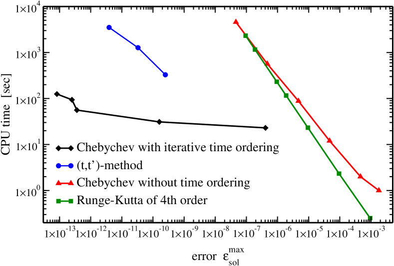
Figure 3: (color online) Comparison of propagation methods for strongly time-dependent Hamiltonian ($\omega_{0}=\omega$) in terms of the CPU time required in order not to exceed a given maximum error of the solution, $\mathrm{\varepsilon_{sol}^{\max}}$.

A clear separation between highly accurate methods (Chebychev propagator with iterative time ordering, $(t,t^{\prime})$ method) and less accurate methods (standard Chebychev propagator without time ordering, fourth-order Runge-Kutta scheme) emerges. If a highly accurate method is desired, the Chebychev propagator with iterative time ordering appears to be the best choice. It outperforms the $(t,t^{\prime})$ method not only in terms of CPU time as shown in Fig. 3 but also in terms of required memory. In the intermediate regime realizing a comprise between accuracy and efficiency, the Chebychev propagator with iterative time ordering is still the best choice. While the less accurate methods that ignore time ordering become prohibitively expensive, the $(t,t^{\prime})$ method does not cover this regime. This is due to the choice of $N_{t^{\prime}}$ – if it is large enough, the calculation is converged and the error is very small, if it is too large, convergence cannot be achieved and norm conservation is violated. Only for cases, where a limited accuracy of the solution is sufficient ($\varepsilon_{\mathrm{sol}}>10^{-5}$), the standard Chebychev propagator and the fourth-order Runge-Kutta scheme represent the most efficient propagation schemes.

IV.3 Wave packet interferometry

Our third example applies the Chebychev propagator with iterative time ordering to a model that cannot be integrated analytically. It explores the effect of time ordering on phase sensitivity as employed in coherent control. Wave packet interferometry has first been demonstrated in the early 1990s.schererJCP91 A pair of electronic or vibrational wave packets are made to interfere by two laser pulses. This represents a conceptually very simple prototype of quantum control.Tannorbook The interference is controlled by the relative phase between the two pulses.

Our example is inspired by a recent experiment.OhmoriPRL06 We consider two harmonic oscillators that are coupled by a laser field,

$$\boldsymbol{\mathsf{\hat{H}}}=\begin{pmatrix}\boldsymbol{\mathsf{\hat{T}}}+\boldsymbol{\mathsf{\hat{V}}}_{g}(r)&\boldsymbol{\mathsf{\hat{\mu}}}E(t)\\ \boldsymbol{\mathsf{\hat{\mu}}}E(t)&\boldsymbol{\mathsf{\hat{T}}}+\boldsymbol{\mathsf{\hat{V}}}_{e}(r)\\ \end{pmatrix}\,,$$ (36)

where $\boldsymbol{\mathsf{\hat{T}}}$ denotes the kinetic energy and

$$\boldsymbol{\mathsf{\hat{V}}}_{g}(r) = \frac{1}{2m}\omega_{g}^{2}r^{2}\,,$$

$$\boldsymbol{\mathsf{\hat{V}}}_{e}(r) = \frac{1}{2m}\omega_{e}^{2}(r-r_{e})^{2}\,.$$

For simplicity we again take $m=1$, $\omega_{g}=\omega_{e}=1$, and $\mu=1\,$a.u. The Hamiltonian is represented on a Fourier grid with $N_{\mathrm{grid}}=128$, $r_{\min}=-10\,$a.u., $r_{\max}=12\,$a.u. and $r_{e}=3.5\,$a.u. Starting from the vibronic ground state, a pump pulse is applied to create a wave packet in the excited state, cf. Fig. 4a. The excited state wave packet oscillates back and forth in the excited state potential with a period of $2\pi/\omega_{e}$. The control pulse, with parameters identical to those of the pump pulse, can be applied with different time delays. If it is applied after one vibrational period, a relative phase equal to zero induces constructive interference while a relative phase of $\pi$ induces destructive interference.Tannorbook Different time delays combined with a different choice of the relative phase yield the same result.Tannorbook Constructive interference implies an increase of population in the excited state, while for destructive interference the wave packet is deexcited to the ground state.

The excited state population that was measured in the experiment by a probe pulse,OhmoriPRL06 can be simply calculated, $|\langle\psi_{e}|\psi_{e}\rangle|^{2}$. The ratio of excited state population at the final time $T$ and at time $t_{1}$, just after the pump pulse,

$$R(\varphi)=\frac{|\langle\psi_{e}(T)|\psi_{e}(T)\rangle|^{2}}{|\langle\psi_{e}(t_{1})|\psi_{e}(t_{1})\rangle|^{2}}\,,$$ (37)

depends on the relative phase between the two pulses, $\varphi$. This dependence is illustrated in Fig. 4b.

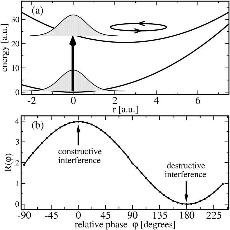
Figure 4: (a) Schematic representation of the generation of wave packets in the excited state with an ultrashort laser pulse. (b) Ratio of the population on the excited state as a function of the relative phase between the pump and the control pulse. $t_{1}$ is the end of the pump pulse.

For $\varphi=0$, the population increases by a factor of four and for $\varphi=\pi$ complete de-excitation is observed.

Since an analytical solution is not available for this example, we take the solution obtained by the Chebychev propagator with iterative time ordering as the reference. The accuracy of propagators without time ordering is analyzed in terms of the relative error $\varepsilon_{sol}^{rel}$,

$$\varepsilon_{sol}^{rel}(\varphi)=\frac{|R_{ITO}(\varphi)-R(\varphi)|}{R_{ITO}(\varphi)}\,.$$ (38)

They are shown for the standard Chebychev propagator, the split propagator and the fourth-order Runge-Kutta scheme in Figs. 5 and 6 for different pulse energies (respectively, pulse areas) and $\Delta t=10^{-4}\,$a.u. (which has to be compared to the duration of the pulse, $0.3\,$a.u. and the vibrational period, $2\pi\,$a.u.).

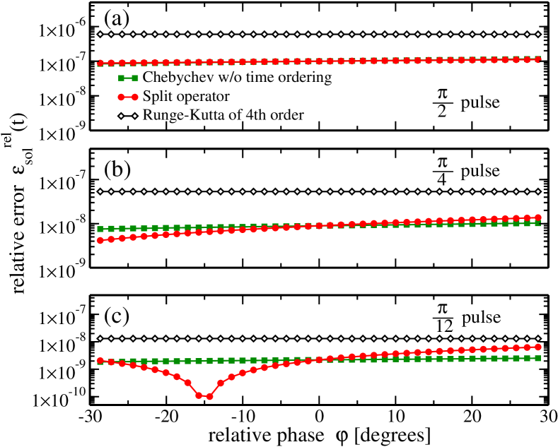
Figure 5: (color online) Constructive wave packet interference: Accuracy of the standard Chebychev propagator, the split propagator and the 4th order Runge-Kutta scheme with respect to the Chebychev propagator with iterative time ordering for different pulse areas.

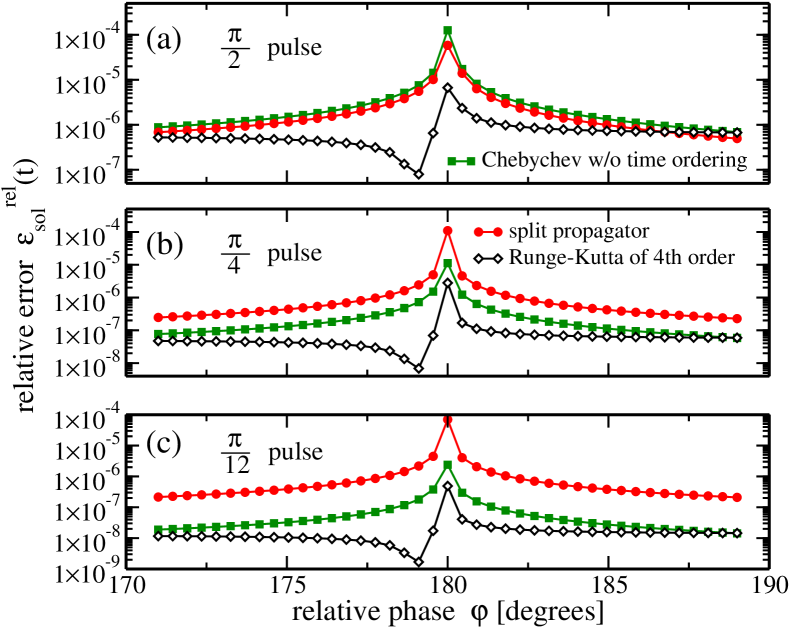
Figure 6: (color online) Destructive wave packet interference: Accuracy of the standard Chebychev propagator, the split propagator and the 4th order Runge-Kutta scheme with respect to the Chebychev propagator with iterative time ordering for different pulse areas.

Fig. 5 corresponds to (almost) constructive interference, $\varphi\approx 0$, Fig. 6 to (almost) destructive interference, $\varphi\approx\pi$. Overall, the relative errors obtained are smaller for wave packet interference compared to the examples of the previous sections IV.1 and IV.2. We attribute this to the fact that the pump and control pulse are very short compared to the vibrational time scale of the oscillators. In this regime of impulsive excitation, the pulses act almost as $\delta$-functions, and there is not enough time to accumulate large errors due to neglected time ordering. However, even in this regime the errors are non-negligible. As expected the errors become larger with increasing pulse intensity. The Runge-Kutta scheme yields similar errors for both constructive and destructive interference. The results obtained by the standard Chebychev propagator without time-ordering and the split propagator appear to be only weakly affected by time ordering for constructive inteference. The results obtained with these two propagators for destructive interference are much more sensitive to time ordering effects and relative errors reach between $10^{-6}$ and $10^{-4}$ for weak and strong pulses, respectively. The error of the split propagator is due to two effects – time-ordering and the non-vanishing commutator between kinetic and potential energy while the error of the standard Chebychev propagator is solely due to time ordering. For weak pulses, the standard Chebychev propagator yields more accurate results than the split propagator, cf. Fig. 6. However, for strong pulses (pulse area of $\pi/2$) roughly the same accuracy is achieved by the standard Chebychev propagator and the split propagator. This indicates that the neglected time-ordering becomes the dominating source of error.

V Conclusions

We have developed a Chebychev propagator based on iterative time ordering to solve TDSEs with an explicitly time-dependent Hamiltonian. The key idea consists in rewriting the term of the TDSE that contains the time-dependence of the Hamiltonian as an inhomogeneity. This inhomogeneity can be approximated iteratively. At each step of the iteration, the Chebychev propagator for inhomogeneous Schrödinger equationsNdongJCP09 is employed. Convergence is reached when the wave functions of two consecutive iteration steps differ by less than a pre-specified error. Time ordering is thus accomplished in an implicit manner.

We have outlined the implementation of the algorithm and demonstrated the accuracy and efficiency of this propagator for three different examples. A comparison to analytical solutions and other available propagators has shown our approach to be extremely accurate, yet efficient, in particular for very strong time dependencies.

The importance of correctly accounting for time ordering effectsKormannJCP08 has been demonstrated for destructive quantum interference phenomena. In most of the literature on coherent control, accurate propagation methods are employed but time ordering effects are completely neglected. This is not justified, in particular for applications such as optimal control theory or high-harmonic generation where the fields are very strong.

The approach of rewriting parts of the TDSE as an inhomogeneity can be extended to other classes of problems where numerical integration is difficult. An obvious example is given by non-linear Schrödinger equations such as the Gross-Pitaevski equation. By rewriting the non-linear term as an inhomogeneity, it should be possible to derive a very stable propagation scheme.

Appendix A Transformation to obtain the coefficients $|\Phi^{(j^{\prime})}\rangle$ from the Chebychev expansion coefficients $|\bar{\Phi}_{j}\rangle$ of the inhomogeneous term

In order to make use of Eq. (14), a transformation linking the Chebychev coefficients, $|\bar{\Phi}_{j}\rangle$ that are calculated by cosine transformation of the inhomogeneous term, cf. Eq. (13), to the coefficients $|\Phi^{(j^{\prime})}\rangle$ appearing in the formal solution of the inhomogeneous Schrödinger equation, cf. Eqs. (15)-(II.2), is required. Assuming $\tau\in[0,t]$, then $\bar{\tau}=2\tau/t-1$, and Eq. (14) becomes

$$\sum_{j=0}^{m-1}P_{j}(\bar{\tau})|\bar{\Phi}_{j}\rangle=\sum_{j^{\prime}=0}^{m-1}\frac{\tau^{j^{\prime}}}{j^{\prime}!}|\Phi^{(j^{\prime})}\rangle\,.$$ (39)

Replacing $\tau$ by $\bar{\tau}$ in the right-hand side of (39), one obtains

$$\sum_{j=0}^{m-1}P_{j}(\bar{\tau})|\bar{\Phi}_{j}\rangle=\sum_{j^{\prime}=0}^{m-1}\frac{(\bar{\tau}+1)^{j^{\prime}}t^{j^{\prime}}}{j^{\prime}!2^{j^{\prime}}}|\Phi^{(j^{\prime})}\rangle\,.$$ (40)

The Chebychev polynomials can be expanded in powers of $\bar{\tau}$,

$$P_{j}(\bar{\tau})=\sum_{k=0}^{j}C_{j,k}\frac{\bar{\tau}^{k}}{k!}\,.$$ (41)

Since Chebychev polynomials satisfy

$$P_{j+1}(\bar{\tau})=2\bar{\tau}P_{j}(\bar{\tau})-P_{j-1}(\bar{\tau})\,,$$ (42)

the coefficients $C_{j,k}$ satisfy a corresponding recursion relation, cf. Eq. (A6) of Ref. NdongJCP09, . Inserting Eq. (40) into Eq. (39) yields

$$\sum_{j=0}^{m-1}\sum_{k=0}^{j}\frac{C_{j,k}}{k!}|\bar{\Phi}_{j}\rangle\bar{\tau}^{k}=\sum_{j^{\prime}=0}^{m-1}\sum_{k=0}^{j^{\prime}}\frac{j^{\prime}!}{k!(j^{\prime}-k)!}\frac{t^{j^{\prime}}}{j^{\prime}!2^{j^{\prime}}}|\Phi^{(j^{\prime})}\rangle\bar{\tau}^{k}\,.$$ (43)

Introducing

$$|\bar{\alpha}_{j,k}\rangle = \frac{C_{j,k}}{k!}|\bar{\Phi}_{j}\rangle\,,$$

$$|\beta_{j^{\prime},k}\rangle = \frac{1}{k!(j^{\prime}-k)!}\frac{t^{j^{\prime}}}{2^{j^{\prime}}}|\Phi^{(j^{\prime})}\,,$$

Eq. (43) is rewritten

$$\sum_{j=0}^{m-1}\sum_{k=0}^{j}|\bar{\alpha}_{j,k}\rangle\bar{\tau}^{k}=\sum_{j^{\prime}=0}^{m-1}\sum_{k=0}^{j^{\prime}}|\beta_{j^{\prime},k}\rangle\bar{\tau}^{k}\,.$$ (44)

Calculation of the $|\Phi^{(j^{\prime})}\rangle$ from the $|\bar{\Phi}_{j}\rangle$ is thus equivalent to calculate the $|\beta_{j^{\prime},k}\rangle$ from the $|\bar{\alpha}_{j,k}\rangle$. Note that the powers of $\bar{\tau}$ in Eq. (44) occur in the inner sums. In order to transform them to the outer sums, first the left-hand side of Eq. (43) is written

$$\sum_{j=0}^{m-1}\sum_{k=0}^{j}\frac{C_{j,k}}{k!}|\bar{\Phi}_{j}\rangle\bar{\tau}^{k} = |\bar{\alpha}_{0,0}\rangle+\sum_{k=0}^{1}|\bar{\alpha}_{1,k}\rangle\bar{\tau}^{k}+\sum_{k=0}^{2}|\bar{\alpha}_{2,k}\rangle\bar{\tau}^{k}+\cdots+\sum_{k=0}^{m-1}|\bar{\alpha}_{m-1,k}\rangle\bar{\tau}^{k}\,,$$ (45)

$$\sum_{j=0}^{m-1}\sum_{k=0}^{j}\frac{C_{j,k}}{k!}|\bar{\Phi}_{j}\rangle\bar{\tau}^{k} = \sum_{j=0}^{m-1}|\bar{\alpha}_{j,0}\rangle+\sum_{j=1}^{m-1}|\bar{\alpha}_{j,1}\rangle\bar{\tau}+\sum_{j=2}^{m-1}|\bar{\alpha}_{j,2}\rangle\bar{\tau}^{2}+\cdots+|\bar{\alpha}_{m-1,m-1}\rangle\bar{\tau}^{m-1}\,,$$ (46)

$$\sum_{j=0}^{m-1}\sum_{k=0}^{j}\frac{C_{j,k}}{k!}|\bar{\Phi}_{j}\rangle\bar{\tau}^{k} = \sum_{j=0}^{m-1}\sum_{k=j}^{m-1}|\bar{\alpha}_{j,k}\rangle\bar{\tau}^{j}\,.$$ (47)

Similarly, the right-hand side of Eq. (43) is written

$$\sum_{j^{\prime}=0}^{m-1}\sum_{k=0}^{j^{\prime}}\frac{1}{k!(j^{\prime}-k)!}\frac{t^{j^{\prime}}}{2^{j^{\prime}}}|\Phi^{(j^{\prime})}\rangle\bar{\tau}^{k}=\sum_{j^{\prime}=0}^{m-1}\sum_{k=j^{\prime}}^{m-1}|\beta_{j^{\prime},k}\rangle\bar{\tau}^{j^{\prime}}\,.$$ (48)

Equating the right-hand sides of Eq. (47) and Eq. (48), the $|\beta_{j^{\prime},k}\rangle$ are obtained,

$$\sum_{j^{\prime}=k}^{m-1}|\beta_{j^{\prime},k}\rangle=\sum_{j=k}^{m-1}|\bar{\alpha}_{j,k}\rangle,\,\,\,\,0\leq k\leq m-1\,.$$ (49)

Replacing $|\bar{\alpha}_{j,k}\rangle$ and $|\beta_{j^{\prime},k}\rangle$ by their definition yields

$$\sum_{j^{\prime}=k}^{m-1}\frac{1}{k!(j^{\prime}-k)!}\frac{t^{j^{\prime}}}{2^{j^{\prime}}}|\Phi^{(j^{\prime})}\rangle = \sum_{j=k}^{m-1}\frac{C_{j,k}}{k!}|\bar{\Phi}_{j}\rangle,\qquad 0\leq k\leq m-1\,,$$

$$\frac{1}{k!}\sum_{j^{\prime}=k}^{m-1}\frac{1}{(j^{\prime}-k)!}\frac{t^{j^{\prime}}}{2^{j^{\prime}}}|\Phi^{(j^{\prime})}\rangle = \frac{1}{k!}\sum_{j=k}^{m-1}C_{j,k}|\bar{\Phi}_{j}\rangle,\qquad 0\leq k\leq m-1\,,$$ (50)

$$\sum_{j^{\prime}=k}^{m-1}\frac{1}{(j^{\prime}-k)!}\frac{t^{j^{\prime}}}{2^{j^{\prime}}}|\Phi^{(j^{\prime})}\rangle = \sum_{j=k}^{m-1}C_{j,k}|\bar{\Phi}_{j}\rangle\,,\qquad 0\leq k\leq m-1\,.$$

This leads to the hierarchy of equations

$$\frac{t^{m-1}}{2^{m-1}}|\Phi^{(m-1)}\rangle = C_{m-1,m-1}|\bar{\Phi}_{m-1}\rangle\,,$$

$$\frac{t^{m-2}}{2^{m-2}}|\Phi^{(m-2)}\rangle+\frac{t^{m-1}}{2^{m-1}}|\Phi^{(m-1)}\rangle = C_{m-2,m-2}|\bar{\Phi}_{m-2}\rangle+C_{m-1,m-2}|\bar{\Phi}_{m-1}\rangle\,,$$

$$\vdots = \vdots$$

$$\sum_{j^{\prime}=k}^{m-1}\frac{1}{(j^{\prime}-k)!}\frac{t^{j^{\prime}}}{2^{j^{\prime}}}|\Phi^{(j^{\prime})}\rangle = \sum_{j=k}^{m-1}C_{j,k}|\bar{\Phi}_{j}\rangle,\qquad 0\leq k\leq m-2\,.$$ (51)

The coefficients $|\Phi^{(j^{\prime})}\rangle$ can thus be determined step by step from the coefficients of the Chebychev expansion, $|\bar{\Phi}_{j}\rangle$,

$$|\Phi^{(m-1)}\rangle = \frac{2^{m-1}}{t^{m-1}}C_{m-1,m-1}|\bar{\Phi}_{m-1}\rangle\,,$$ (52)

$$|\Phi^{(k)}\rangle = \frac{2^{k}}{t^{k}}\left(\sum_{j=k}^{m-1}C_{j,k}|\bar{\Phi}_{j}\rangle-\sum_{j=k+1}^{m-1}\frac{1}{(j^{\prime}-k)!}\frac{t^{j^{\prime}}}{2^{j^{\prime}}}|\Phi^{(j^{\prime})}\rangle\right)\,,\qquad k=m-2,0\,.$$ (53)

Note that the transformation given by Eqs. (52) and (53) becomes numerically instable for large orders, $m\sim 100$. In our applications, such a large $m$ would correspond to time steps larger than the overall propagation time and was never required.

References

- (1) M. Lewenstein, P. Balcou, M. Y. Ivanov, A. L’Huillier, and P. B. Corkum, Phys. Rev. A 49, 2117 (Mar 1994).
- (2) J. Itatani, D. Zeidler, J. Levesque, M. Spanner, D. M. Villeneuve, and P. B. Corkum, Phys. Rev. Lett. 94, 123902 (Mar 2005).
- (3) H. Dietz and V. Engel, J. Phys. Chem. A 102, 7406 (1998).
- (4) Ronnie Kosloff, Stuart A. Rice, Pier Gaspard, Sam Tersigni and David Tannor, Chem. Phys. 139, 201 (1989).
- (5) W. Zhu, J. Botina, and H. Rabitz, J. Chem. Phys. 108, 1953 (1998).
- (6) S. Blanes, F. Casas, J. A. Oteo, J. Ros, Phys. Rep. 470, 151 (2009).
- (7) W. Magnus, Commun. Pure Appl. Math 7, 649 (1954).
- (8) Hillel Tal-Ezer, Ronnie Kosloff, and Charly Cerjan, J. Comp. Phys. 100, 179 (1992).
- (9) Charly Cerjan and Ronnie Kosloff, Phys. Rev. A 47, 1852 (1993).
- (10) M. Klaiber, D. Dimitrovski, and J. S. Briggs, Phys. Rev. A 79 (2009).
- (11) U. Peskin, R. Kosloff, and N. Moiseyev, J. Phys. Chem. 100, 8849 (1994).
- (12) R. Kosloff, J. Phys. Chem. 92, 2087 (1988).
- (13) A. Bandrauk and H. Shen, Chem. Phys. Lett. 176, 428 (1991).
- (14) R. Fischer, A. Staudt, and C. Keitel, Comp. Phys. Commun. 157, 139 (2004).
- (15) A. Bandrauk, E. Dehghanian, and H. Lu, Chem. Phys. Lett. 419, 346 (2006).
- (16) Y. Ohtsuki, H. Kono, and Y. Fujimura, J. Chem. Phys. 109, 9318 (1998).
- (17) Y. Ohtsuki and K. Nakagami, Phys. Rev. A 77 (2008).
- (18) M. Hsieh and H. Rabitz, Phys. Rev. E 77 (2008).
- (19) C. Gollub and R. de Vivie-Riedle, Phys. Rev. A 78, 033424 (2008).
- (20) A. S. Leathers, D. A. Micha, and D. S. Kilin, J. Chem. Phys. 131, 144106 (2009).
- (21) J. C. Tremblay and J. Tucker Carrington, J. Chem. Phys. 121, 11535 (2004).
- (22) C. P. Koch, J. P. Palao, R. Kosloff, and F. Masnou-Seeuws, Phys. Rev. A 70, 013402 (2004).
- (23) M. D. Feit, J. A. Fleck, and A. Steiger, J. Comput. Phys. 47, 412 (1982).
- (24) K. Kormann, S. Holmgren, and H. O. Karlsson, J. Chem. Phys. 128, 184101 (2008).
- (25) Claude Leforestier, Rob Bisseling, Charly Cerjan, Michael Feit, Rich Friesner, A. Guldberg, Audrey Dell Hammerich, G. Julicard, W. Karrlein, Hans Dieter Meyer, Nurit Lipkin, O. Roncero and Ronnie Kosloff, J. Comp. Phys. 94, 59 (1991).
- (26) M. Ndong, H. Tal-Ezer, R. Kosloff, and C. P. Koch, J. Chem. Phys. 130, 124108 (2009).
- (27) R. Baer, Phys. Rev. A 62, 063810 (2000).
- (28) If the Chebychev coefficients can be calculated based on an analytical expression, the smallest Chebychev coefficient itself can be pushed below machine precision. This is the case, for example, for the standard Chebychev propagator where the expansion coefficients of the function are given in terms of Bessel functions. Here, our accuracy is limited to the relative error specified by Eq. (26) because the expansion coefficients can only be obtained numerically by fast cosine transformation.
- (29) L. C. Allen and J. H. Eberly, Optical Resonance and Two-Level Atoms (Dover, 1988).
- (30) Y. I. Salamin, J. Phys. A. Math. Gen. 28, 1129 (1995).
- (31) R. Kosloff, Annu. Rev. Phys. Chem. 45, 145 (1994).
- (32) I. Kondov, U. Kleinekathöfer, and M. Schreiber, J. Chem. Phys. 114, 1497 (2000).
- (33) N. F. Scherer, R. J. Carlson, A. Matro, M. Du, A. J. Ruggiero, V. Romero-Rochin, J. A. Cina, G. R. Fleming, and S. A. Rice, J. Chem. Phys. 95, 1487 (1991).
- (34) D. J. Tannor, Introduction to Quantum Mechanics. A time-dependent perspective (Palgrave MacMillan, 2007).
- (35) K. Ohmori, H. Katsuki, H. Chiba, M. Honda, Y. Hagihara, K. Fujiwara, Y. Sato, and K. Ueda, Phys. Rev. Lett. 96, 093002 (2006).