Comment on “Electron transport through correlated molecules computed using the time-independent Wigner function: Two critical tests”

Abstract

The many electron correlated scattering (MECS) approach to quantum electronic transport was investigated in the linear response regime [I. Bâldea and H. Köppel, Phys. Rev. B. 78, 115315 (2008)]. The authors suggest, based on numerical calculations, that the manner in which the method imposes boundary conditions is unable to reproduce the well-known phenomena of conductance quantization. We introduce an analytical model and demonstrate that conductance quantization is correctly obtained using open system boundary conditions within the MECS approach.

I Introduction

Electron transport calculations in the linear response regime for a method referred to as the stationary Wigner function (SWF) method have been reported [I. Bâldea and H. Köppel, Phys. Rev. B. 78, 115315 (2008)], as a shorthand we will refer to their presentation as BK. In fact though, their paper is a comment on the validity of a method introduced by Delaney and Greer DeG04a for treating open system boundary conditions for correlated many-electron problems, or many-electron correlated scattering (MECS) DeG04a ; ASS06 ; MGF09 . For reasons that will hopefully become clear, we refer to the method under discussion as MECS SWF . BK express several criticisms of the MECS method, but their primary objection and conclusion is

“… the manner in which it” (open system boundary conditions through the Wigner function) “was imposed in” [P. Delaney and J.C. Greer, Phys. Rev. Lett. 93, 036805 (2004)] “turns out to be inappropriate. It misses the fact that, in accord with our physical understanding, the current flow is due to an asymmetric injection of electrons from reservoirs into the device, and that injected electrons are very well described by Fermi distributions with different chemical potentials. Moreover, as results from the analysis at the end of Sec. VI” (of the BK paper), “unfortunately there is no simple remedy of the SWF method; the modification of the boundary conditions in the spirit of” Delaney and Greer “such as to account for a nonvanishing chemical potential shift does not yield the desired improvement.”

The conclusion in BK is reached after numerical calculations on a test system designed to model independent electron and correlated electron transport across a quantum dot. As we will demonstate, their conclusion incorrectly presumes an asymmetric injection of momentum is necessary to describe reservoirs or electrodes in quasi-equilibrium, and likewise incorrectly assumes there is no chemical potential difference when applying the open system boundary conditions with the MECS procedure. We will show that the Wigner boundary conditions as expressed for MECS calculations, or equally in previous works Fre90 , is consistent with the application of a “non-vanishing chemical potential shift”. The authors in their paper appear to be confusing the application of open boundary conditions when using either energy or momentum distributions, and we will clarify that a relative shift in energy to the reservoir energy distributions does not imply a shift for the corresponding momentum distributions emitted into a scattering region for simple models of electrode behaviour.

In sect. II, we give a brief overview of the MECS method. This is followed in sect. III by introduction of a resolution to the apparent conundrum expressed by BK: we analyse momentum distributions for electron reservoirs or electrodes represented by Fermi-Dirac distributions and observe that the momenta distributions do not change with applied voltage bias, or equivalently with a chemical potential imbalance applied between electrodes. Asymmetric injection implied by BK’s conclusion in relation to the momentum distributions from the electrodes is not consistent with a MECS or a Landauer description of electron transport. In sect. IV, a calculation of conductance quantization for a system with the electrodes represented by parabolic energy bands in one spatial dimension is given using the MECS construction. To clearly identify how the boundary conditions can be treated in this case, electron interactions are neglected and the method reduces to a many-electron scattering problem for non-interacting electrons. This approximation has the advantage of highlighting the simplicity of the MECS formulation as well as clearly demonstrating its consistency with standard formulations of electron scattering, while avoiding issues related to specific numerical approximations or questions related to specific electronic structure implementations. The boundary conditions as formulated in MECS applied to the model reproduces the well-known result of conductance quantization.

II A brief introduction to the MECS approach

The proposal behind MECS as introduced in ref. DeG04a is to constrain a many-electron wavefunction on a scattering region, or specifically, the many-electron density matrix (DM)

$$\rho_{N}=|\Psi_{N}><\Psi_{N}|,$$ (1)

in a manner satisfying open system boundary equations Fre90 . As open system boundary conditions are commonly expressed in the language of single particle theories, it is useful to consider the Wigner transform of the one-electron reduced density matrix (RDM) associated with the many-electron DM

$$\rho_{N} \rightarrow \rho_{1},\,\,\,\,{\rm with}\,\,\,\,{\rm Tr}\rho_{1}=N$$

$$f_{W}(q,p) = \int_{-\infty}^{+\infty}dr\,\exp(-ipr/\hbar)\rho_{1}(q-r/2;q+r/2),$$ (2)

where here the transform is written for one spatial dimension $r$ and $\{p,q\}$ are Wigner phase space variables. The MECS approach is the recognition that open system boundary conditions can be applied to correlated systems through the one-body RDM through use of the Wigner transform, allowing appropriate conditions to be enforced at the boundaries of a scattering region. In practice, the Wigner distribution function is used to constrain the momenta flow out of the electron reservoirs and into the scattering region. The momentum expection value can be written as

$$<p>=\frac{1}{2\pi\hbar}\int_{-\infty}^{+\infty}dp\,dq\,\,p\,f_{W}(q,p).$$ (3)

Eq. 3 highlights the analogy of the Wigner quantum phase space distribution to a classical probability distribution function. However, unlike a classical probability distribution and as is well known Fre90 ; CaZ83 ; HOS84 ; Lee95 , the Wigner function is not everywhere positive as a consequence of the Heisenberg momentum-position uncertainty principle. However, in regions where $f_{W}$ behaves approximately classically, the Wigner phase representation allows us to assign meaning to phrases such as “electrons in the left or right reservoir”, “momentum of an electron emitted from a reservoir”, or “a reservoir is locally in equilibrium”. Within this context, the net momentum flow out of the left electrode is approximated as

$$p_{l}=\frac{1}{2\pi\hbar}\int_{0}^{+\infty}dp\,\,p\,\,f_{W}(q_{l},p),$$ (4)

and similarly for the right electrode

$$p_{r}=\frac{1}{2\pi\hbar}\int_{-\infty}^{0}dp\,\,p\,\,f_{W}(q_{r},p)$$ (5)

where $q_{l}$ and $q_{r}$ are appropriately chosen. Clearly this approximation is dependent upon how well $f_{W}$ describes a classical probability distribution function. For metal electrodes, where electrons can be well approximated by the free electron model, this assumption is usually justified. It is also noteworthy that the Wigner reduced one-particle function, as a function of energy defined in the Wigner phase space, tends rapidly toward the Fermi-Dirac distribution with increasing number of particles in a confining potential CBJ07 .

In our calculations to date, three-dimensional electrodes are considered DeG04a ; MGF09 ; FDG06 ; FaG07 . To simplify the analysis, $f_{W}$ is integrated over the in-plane coordinates within a cross section of the electrodes. The net momentum flow out of both electrodes is constrained to this equilibrium ($V=0$) value DeG04a ; DeG04b . To consider this procedure further, we examine models of electrode behaviour in quantum transport theories.

III Fermi-Dirac reservoir energy and momentum distributions under applied voltage at zero temperature

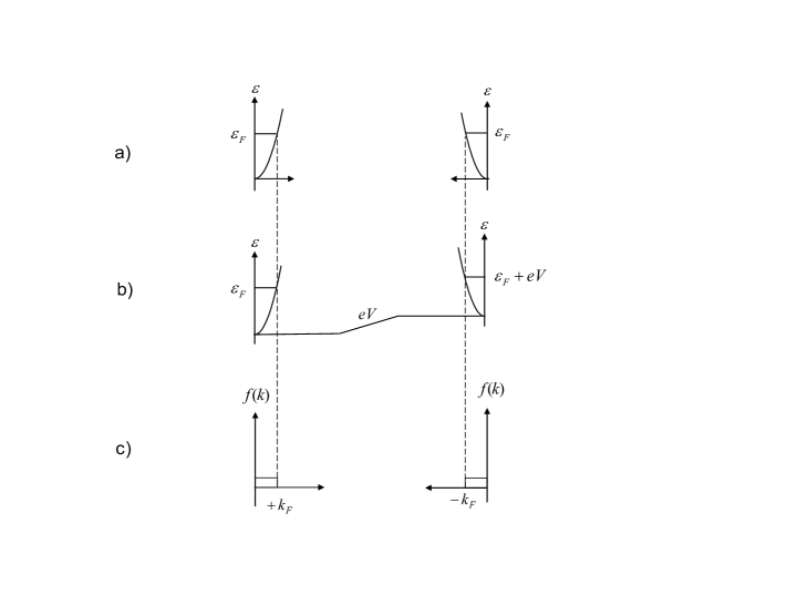
Figure 1: The Fermi-Dirac energy dispersions for incoming electrons from two electrodes described by parabolic bands. a) with no voltage difference between the electrodes, b) with applied voltage. c) The corresponding momentum distribution functions for a) and b). Note that there is no difference to the momentum distributions with application of voltage.

In fig. 1a), a pictorial representation of open system boundary conditions is shown for electrodes described by two parabolic energy bands (free-electrons with effective mass $m^{*}$ in one dimension and for a Fermi-Dirac distribution at temperature $T=0$). The energy levels $\epsilon_{k}=\frac{(\hbar k)^{2}}{2m^{*}}$ in the left and right electrodes are filled to the Fermi energy $\epsilon_{F}$; similarly momentum states are filled to the Fermi momentum $k_{F}$. In fig. 1b), a potential energy difference is introduced between the left and right electrodes shifting the bottom of the energy bands with respect to each other by an amount denoted $eV$. This results in a shift to the energies in the right electrode by $\frac{(\hbar k)^{2}}{2m^{*}}\rightarrow\frac{(\hbar k)^{2}}{2m^{*}}+eV$ (a symmetric split in the voltage between electrodes does not alter our discussion). The shift of the right electrode energy states describes the chemical potential imbalance between the reservoirs and will necessarily be accompanied by a voltage drop, or equivalently an electric field across the scattering region. In fig. 1c), the momentum distributions corresponding to Fermi-Dirac energy distributions with and without applied voltage in fig. 1a) and fig. 1b), respectively, are shown. The same momentum distributions are obtained with or without application of a voltage difference between the left and right electrodes. It also follows that similar considerations hold for the case of non-zero temperature. It is important to highlight at this point that the MECS proposal DeG04a for treating quantum electronic transport is completely compatible with this picture of boundary conditions on the electrode regions.

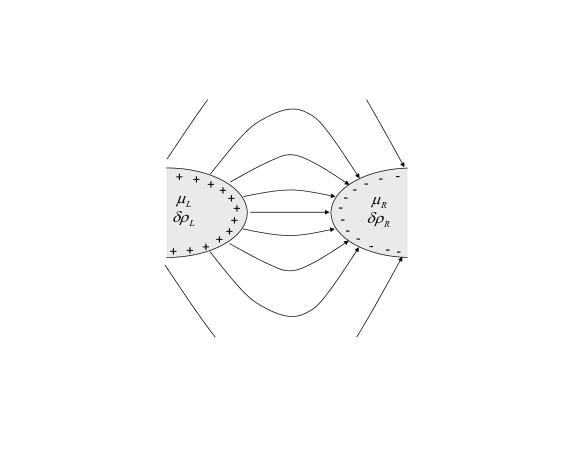
Figure 2: A simple model of the action of two electrodes in generating an electric field. The application of a chemical potential difference results in surface charges generating an electric field between the electrodes.

When working with the one-electron RDM obtained from a correlated $N$-electron density matrix, it is not possible to unambiguously define single electron energies. It is therefore of advantage to constrain the total incoming momentum to model the action of the electrodes while determining the correlated many-electron density matrix on the scattering region. As the incoming momentum distributions are the same for electrodes in equilibrium or in local equilibrium, constraining the net momentum flow from the electrodes is not sufficient to drive the electrodes away from equilibrium with respect to each other. It is standard practice in many electron transport methods, including non-equilibrium Green’s function (NEGF) techniques, to introduce an external electric field to model the action of the electrodes on the scattering region. To understand the role of the external field in transport calculations, it is useful to consider the sketch of two metallic electrodes as presented in fig. 2. A simple band or independent particle model is a remarkably good approximation to the electronic structure of metals allowing our discussion of the parabolic bands to be extended directly to consideration of realistic models of metal electrodes. Within fig. 2, the fact that the two electrodes are not in equilibrium with respect to one another is denoted by the different left $\mu_{L}$ and right $\mu_{R}$ chemical potentials. The chemical potential imbalance introduces a difference in the charge density between the left and right electrodes. However, electrostatic screening is efficient in metals and for the quasi-equilibrium regions of the electrodes, the electric field is zero within the electrodes or equivalently, the voltage is constant within a short distance into the metal electrodes. Thus all of the voltage drop is across the scattering region plus the screening length into the electrodes. Typical screening lengths in metals are of the order of 0.1 nm. Hence any charge imbalance in the electrodes resides at the surface of the metal and the opposite polarity of the surface induced charges between the electrodes gives rise to an electric field across the region situated between the electrodes; a situation depicted in fig. 2 as field lines between the electrode surfaces. In most transport calculations, charges in the electrode and scattering regions are solved for self-consistently allowing a molecular tunnel junction to polarize in response to this external electric field. In MECS, charges re-arrange due to minimization of the energy with respect to the many-electron wavefunction subject to the open system boundary conditions and the external electric field. The voltage can then be extracted as the combined field arising from the applied field and polarized charge distribution in the scattering region; see for example BMO02 .

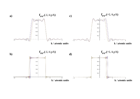
Figure 3: The Wigner function calculated with scattering wavefunctions defined on a region $[-L/2,+L/2]$ and with normalization chosen such that a completely occupied state is with $f=1$. a) The Wigner function calculated at $q_{l}=-L/4$ for a region of length $L=2$ nm with $k_{F}$=0.12 nm^-1=0.635 a.u (corresponding to gold electrodes) with $V$= 0 (blue), 1 (purple), 2 (green) volts. b) Same as in a) but with $L$=20 nm. c) The Wigner function calculated at $q_{r}=+L/4$, otherwise the same as in a). d) Same as in c), but with $L$=20 nm.

The model of electrode behaviour we are describing is consistent with other formulations of quantum electronic transport. In this regard, it is worthwhile to mention the work of McLennan, Lee and Datta MLD91 and in particular their fig. 3. As pointed out by the authors, a change in the chemical potential in the electrodes is accompanied by a shift in the electrostatic voltage. In a metal, the case considered for MECS calculations to date, the chemical potential and electrostatic voltage changes are nearly identical and the effect of the applied voltage can be accounted for as a shift in the electrode bands with respect to each other. In the linear response regime, the shift due to the electrostatic voltage is sometimes neglected MLD91 but formally should be included as indicated schematically in our fig. 1 and in McLennan et al’s fig. 3.

The point which we would like to emphasize is that the presence of voltage drop on the scattering regions ensures that the single electron energies in the electrodes are shifted by the applied voltage, but does not alter the momentum distributions emitted from the electrodes. The conclusion in BK that an asymmetric injection of electrons is needed to obtain a current is incorrect, if injection refers to incoming electron momentum distributions, i.e. ‘current injected’ from the electrodes. What is required is asymmetric scattering for injected electrons, and this is provided for by the asymmetric electric field profile or equivalently, the chemical potential imbalance generated across a molecular tunnel junction.

IV Application of MECS to a single particle model

IV.1 Boundary conditions

MECS was originally formulated for interacting many-electron systems with a Hamiltonian operator given as

$$H_{N}=T+V_{1}+V_{2}$$ (6)

where $T$ is the sum of $N$ one-electron kinetic energy operators, $V_{1}$ is the sum of the external one-electron potentials and $V_{2}$ is the sum of electron-electron interactions on the scattering region DeG04a . As mentioned, with the MECS approach an external electric field can be applied to model the chemical potential imbalance between the reservoirs and this term may be included into $V_{1}$. To arrive at a single particle model to be used in our analysis, the electron-electron interactions are ‘switched’ off and, for simplicity, all other external potentials other than the chemical potential imbalance between the electrodes are also ‘switched’ off. As electron-electron interactions are not treated, the resulting many-electron system consists of $N$ non-interacting electrons each described by a single electron Hamiltonian operator. Of course, there is no advantage to apply the MECS method to a non-interacting electron model, but we demonstrate in this case that the MECS method is consistent with the usual formulation of quantum mechanical scattering.

We consider a scattering region of length $[-L/2,L/2]$ in the absence of a potential and write plane wave eigenfunctions on the scattering region

$$\psi_{n}(x) = \frac{1}{\sqrt{L}}\exp(ik_{n}x)$$

$$k_{n} = 2\pi n/L\,\,\,\,\,\,;\,\,n=\pm 1,\pm 2,\pm 3,\ldots$$ (7)

Left going and right going states are filled to a Fermi momentum $k_{F}=n_{F}\Delta k$. In the absence of the application of a voltage, the current is given simply as

$$I\left[V=0\right]=-\frac{e\hbar}{m^{*}L}\left(\sum_{n_{l}=1}^{n_{F}}k_{n_{l}}-\sum_{n_{r}=1}^{n_{F}}k_{n_{r}}\right)=0,$$ (8)

where $n_{l}$ and $n_{r}$ denote states associated with the left and right electrodes, respectively. In one dimension, the electron current and current density are equivalent, and the factor $\frac{1}{L}$ indicates our choice of normalization. The model consists of left and right propagating plane wave states with the net current summing to zero. In this representation, the density matrix is diagonal with $n_{n,n^{\prime}}=\delta_{nn^{\prime}}$ for both $n,n^{\prime}\leq n_{F}$ and $n_{n,n^{\prime}}=0$ otherwise. This allows the density matrix to be constructed from the first $n_{F}$ states incoming from the left and right to be written as

$$\rho_{0}(x,x^{\prime})=\frac{1}{L}\sum_{n=1}^{n_{F}}\exp\left[ik_{n}(x-x^{\prime})\right]+\frac{1}{L}\sum_{n=1}^{n_{F}}\exp\left[-ik_{n}(x-x^{\prime})\right].$$ (9)

Introducing the Wigner transformation term by term, the resulting Wigner distribution function is readily found to be

$$f_{0}(q,p)=\sum_{n=1}^{n_{F}}\left[f_{n}(q,p_{n})+f_{n}(q,-p_{n})\right]=\frac{2\pi}{L}\sum_{n=1}^{n_{F}}\delta(p_{n}-\hbar|k_{n}|)+\frac{2\pi}{L}\sum_{n=1}^{n_{F}}\delta(p_{n}+\hbar|k_{n}|),$$ (10)

with $\delta(p)$ the Dirac delta function. Strictly speaking, as we consider wavefunctions that are only non-zero on the scattering region, the delta functions should be replaced by sinc functions of the form: $\frac{1}{\pi(k\pm p/\hbar)}\sin\left[(k\pm p/\hbar)L/2\right]$ that approach delta functions for large $L$. In the case of large $L$, the model as described corresponds to fig. 1a).

Next, a potential step is introduced at $x=0$ to drive the system out of equilibrium and allow for a net current flow. The exact form of the scattering potential is not critical to the following argument, but for ease of presentation we assume that the potential is varied over a small region $l<<L$ allowing us to approximate the difference between the left and right electrodes as a potential energy step. For this case, the solutions to the one-electron Schrödinger equation may be written in scattering form

$$\psi_{n}(x)= \exp(ik_{n}x)+r\exp(-ik_{n}x) x<0$$

$$\psi_{n}(x)= t\exp(ik_{n}^{\prime}x) x>0.$$ (11)

For spatially varying potentials centered at $x=0$ satisfying $l<<L$, the asymptotic wavefunctions will likewise satisfy the scattering form and the following development remains valid with minor modification. By implication, the energies for electrons entering the scattering region from the right are shifted by an amount given by the scattering potential height $\frac{(\hbar k)^{2}}{2m^{*}}\rightarrow\frac{(\hbar k)^{2}}{2m^{*}}+eV$. However the incoming momenta, as previously discussed, are unchanged. We apply a voltage greater than the level spacings at the bottom of the reservoir conduction band where the energy density of states is greatest. With the introduction of the potential, the model for electrons entering from the left is the one-dimensional quantum mechanical scattering problem with a step-up potential. For electrons entering the scattering region from the right, the problem is for an electron incident on a step-down potential. This is shown schematically in fig. 1b) and the solution is well known for both cases and may be expressed in terms of the transmission coefficients $T$. In this case, we can write the current for the system as

$$I\left[V\neq 0\right]=-\frac{e\hbar}{m^{*}L}\sum_{n=1}^{n_{F}}\left[f_{l}(k_{n})T_{l}(k_{n};V)k_{n}-f_{r}(k_{n})T_{r}(k_{n};V)k_{n}\right],$$ (12)

with $T_{l},T_{r}$ the transmission coefficients for electrons incoming from the left and right, respectively. Note that $f_{l,r}(k_{n}\leq k_{F})=1$ and $f_{l,r}(k_{n}>k_{F})=0$ for our example. Time reversal symmetry requires that the left and right transmission functions for a given single particle energy $\epsilon$ are equal $T_{l}(\epsilon)=T_{r}(\epsilon)$, but the energies for the left and right states of equal momentum are not equal in the presence of a voltage. This is seen by re-writing the transmission as functions of energy

$$I\left[V\neq 0\right]=-\frac{e\hbar}{m^{*}L}\sum_{n=1}^{n_{F}}\left[T_{l}\left(\frac{(\hbar k_{n})^{2}}{2m^{*}};V\right)-T_{r}\left(\frac{(\hbar k_{n})^{2}}{2m^{*}}+eV;V\right)\right]k_{n},$$ (13)

resulting in a net current flow with application of voltage.

It can be shown that the Wigner transform of the reduced density matrix constructed from the scattering wave functions satisfies the same open system boundary conditions as the zero voltage (plane-wave states) solution in the large $L$ limit and as we will demonstrate, approximately for finite values of $L$ typically used in numerical studies. The electron reservoirs in this case are the regions outside of the central scattering site. The density matrix with $V\neq 0$ remains diagonal and we can again consider the Wigner transform term by term

$$f_{n,n}(q,p)=\int_{-\infty}^{+\infty}\,dr\,\exp(-ipr/\hbar)\psi_{n}(q+\frac{r}{2})\psi^{*}_{n}(q-\frac{r}{2}).$$ (14)

where now $\psi_{n}$ are wavefunctions of the scattering form eq. IV.1 on $[-L/2,L/2]$. We consider a point to the left of the scattering region $q_{l}=-L/4$ and find for the Wigner distribution function

$$f_{n,n}(q_{l},p)=\frac{2\pi}{L}\delta(p-\hbar k_{n})+\frac{2\pi}{L}r^{2}\delta(p+\hbar k_{n})+\frac{4\pi}{L}r\,\cos(2k_{n}q)\delta(p)$$ (15)

where in eq. 15 $r$ is the amplitude of the reflected component of the scattering wavefunction and the normalization is fixed to that of an incoming plane wave. The Wigner phase space density at $q_{l}$ consists of the incoming momentum term at $p=+\hbar k_{n}$, the reflected momentum term at $p=-\hbar k_{n}$, and a zero mode term $p=0$ as discussed in ref. CaZ83 . The Wigner transform is calculated at $\pm L/4$, in the middle of the electrodes, to avoid coupling to the regions outside of $[-L/2,L/2]$ and to avoid interaction between the electrodes as voltage is applied. If the point where the Wigner function is to be constrained is too close to the boundaries $\pm L/2$, the density matrix, as can be seen from the argument of the Wigner transform eq. 14 $\psi_{n}(\pm L/2+\frac{r}{2})\psi^{*}_{n}(\pm L/2-\frac{r}{2})$, will be zero. The vanishing of the density matrix in this case is an artifact arising from truncating the wavefunctions outside of the scattering region. If the point where the Wigner function is to be constrained is calculated too close to the scattering region, as voltage is applied the incident and reflected components of the scattering wavefunction mix with the transmitted component, or in other words the two electrodes couple. To avoid coupling the electrodes, the Wigner function should be calculated within each electrode, but in a region avoiding interaction between the electrodes as a voltage is applied.

Again, as for eq. 10, for finite $L$ the delta functions in eq. 15 should be replaced by sinc functions of the form $\frac{1}{\pi(k\pm p/\hbar)}\sin\left[(k\pm p/\hbar)L/2\right]$. For large $L$ when the sinc functions well approximate delta functions, eqn. 10 and 15 satisfy the same condition for incoming momenta states. For finite $L$, the sinc functions centered at $\pm k,0$ can overlap and the incoming momentum states can differ between the $V=0$ (plane-wave) and $V\neq 0$ (scattering) states. In fig. 3a), we have calculated the Wigner function for a set of plane wave states incoming from the left and the right with a Fermi momentum $k_{F}$ chosen to correspond to that of gold electrodes and a scattering region of $L=2$ nm. A step potential of $V=0,1,2$ Volts is applied in the center of the scattering region and the resulting Wigner functions are displayed at $q_{l}=-L/4$ for each value of the applied voltage. These parameters have been chosen to compare our analysis to typical calculations for molecular electronics, and in particular the calculation presented in ref. DeG04a . As voltage is applied, the incoming electron distributions are not exactly equal to the $V=0$ distribution, but agreement is very close particularly for states near $k_{F}$ which provide the largest contributions to the current. The outflow of momentum is changed as a result of the scattering off the potential barrier and this difference between the equilibrium ($V=0$) and non-equilibrium distributions ($V\neq 0$) reflects the difference in chemical potential between the electrodes. In fig. 3b), the length of the region is taken to be $L=20$ nm and as seen the incoming momentum distributions, even with wavefunctions only defined on the region $[-L/2,+L/2]$, remain essentially the same for $V=0,1,2$ volts. The momentum distribution drops sharply at $k_{F}$ well approximating the distribution shown in fig. 1c). In fig. 3c) and d), the Wigner distribution at $q_{r}=+L/4$ for $L=$ 2 and 20 nm, respectively, is given. In subsequent discussion, we assume a large value for $L$, but as fig. 3 indicates, the considerations apply well to electrode lengths as small as 1 nm. Also, the lowest $n_{F}$ states have been occupied corresponding to a $T=0$ distribution. However, there is nothing in the analysis that precludes the $V=0$ solution to be set to a thermal distribution and to constrain the solutions to the thermally occupied incoming states as a voltage is applied. If the scattering states with $V\neq 0$ are constrained to satisfy the Wigner function determined from the $V=0$ wavefunctions, the correct solution to the one electron Hamiltonian in the presence of a potential on the scattering region will be obtained in the large $L$ limit and approximately for smaller values of $L$. Indeed it is observed that in the single particle case, constraining the incoming momentum inflow via the Wigner function implies solving the one-electron Schrödinger equation for a specific value of incoming momentum $p=\hbar k_{n}$, and otherwise results in the standard textbook presentation of one-dimensional quantum mechanical scattering.

IV.2 A transport calculation with the single particle model

We again consider introduction of a small potential step to shift the energies of the states incoming from the right, as depicted in fig. 1b). As voltage is applied, electrons incoming from the left with energies such that $\epsilon_{n_{L}}/e<V$ will see a potential step-up. The number of these states is given approximately as

$$n_{V}\approx\sqrt{2em^{*}V}/\hbar\Delta k.$$ (16)

For states incoming from the left, we approximate $T_{l}\sim 0$ for incoming energies less than the potential step height, and $T_{l}\sim 1$ for energies greater than the potential step height. In contrast, electrons incoming from the right see a step-down potential and we approximate $T_{r}\sim 1$ for all electrons incoming from the right. The electron current can then be estimated as

$$I \sim -\frac{e\hbar}{m^{*}L}\left[\sum_{n_{l}=n_{V}}^{n_{F}}k_{n_{l}}-\sum_{n_{r}=1}^{n_{F}}k_{n_{r}}\right]$$ (17)

$$\sim \frac{e\hbar}{m^{*}L}\sum_{n=1}^{n_{V}}k_{n}$$

$$\sim \frac{e\hbar}{m^{*}L}\sum_{n=1}^{n_{V}}n\Delta k,$$

with the convention that current flow is opposite the direction of electron flow. For small $\Delta k$ and large $n_{F}$ (these are standard conditions for derivation of the Landauer formula), we have

$$I\rightarrow\frac{e\hbar}{m^{*}L}\Delta k\int_{0}^{n_{V}}n\,dn=\frac{e^{2}}{h}V.$$ (18)

The current and voltage yield a conductance $g_{0}=e^{2}/h$ and the Landauer result for conductance quantization is obtained.

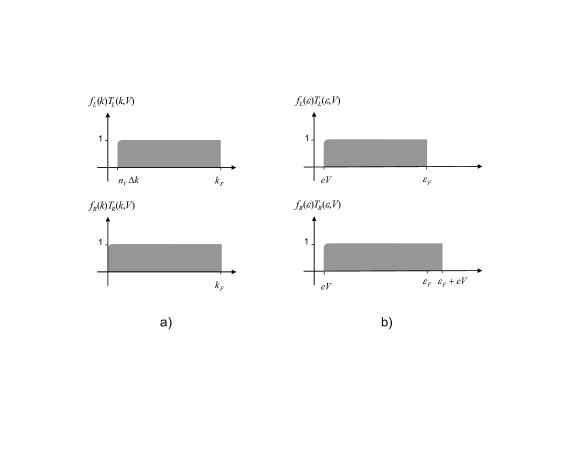
Figure 4: a) The momentum distributions corresponding to the model of sect. IV. b) The energy distributions for the model of sect. IV. Both distributions may be used to calculated conductance quantization.

This derivation seems odd, as it appears that it is not the states at the Fermi level that contribute to the current, but states low in energy (or momentum) that yield a current. The situation can be summarized in fig. 4 . In fig. 4a), the product of the momentum occupation and the transmission coefficients for left and right states are given, whereas in fig. 4b), the corresponding product of the energy level occupations and transmission coefficients are given. In fig. 4a), it appears the currents arise from low momentum states, in fig. 4b), currents appears to arise from energy states at $\epsilon_{F}$. However, there is no contradiction. If the currents from momentum states with energies $\epsilon<\epsilon_{F}$ are summed, the currents associated with states below $\epsilon_{F}$ cancel.

The current incoming from the left can be rewritten as an integral over energy

$$I_{l}=-\frac{e^{2}}{h}\int_{eV}^{\epsilon_{F}}d\epsilon,$$ (19)

using $\epsilon=\frac{(\hbar k)^{2}}{2m^{*}}$ and $d\epsilon=\frac{\hbar^{2}}{m^{*}}k\,dk$. Similarly the current from the right is re-written but now with $\epsilon=\frac{(\hbar k)^{2}}{2m^{*}}+eV$

$$I_{r}=\frac{e^{2}}{h}\int_{eV}^{\epsilon_{F}+eV}d\epsilon.$$ (20)

The resulting current is

$$I=\frac{e^{2}}{h}\int_{\epsilon_{F}}^{\epsilon_{F}+eV}d\epsilon=\frac{e^{2}}{h}V,$$ (21)

which will be recognized as the more familiar form for expressing conductance quantization. The physics is consistent whether calculating currents using the momentum distributions fig. 4a) or the energy distributions fig. 4b).

V Discussion

The first point of our presentation is that the MECS approach is consistent with a Landauer description of electron transport. BK’s conclusion ascribes the failure of their calculations for a single particle and a correlated model to the MECS formulation of boundary conditions. The analysis of sect. III highlights this is not the case; based on an analytical model, the use of the MECS formulation is consistent with a scattering approach to electron transport. The advantage of an analysis based upon an analytical model is that it avoids issues associated with linear response approximations, perturbation theory, variational methods in a finite basis, specific implementations of electronic structure, or other numerical approximations, thereby allowing a clear focus on the physical assumptions made when using the method. In sect. IV, we continue in this vein and demonstrate how the MECS formulation reproduces conductance quantization in a system of non-interacting electrons scattering off a potential barrier.

We would also like to touch upon some formal points raised in the BK work. The authors criticize the use of a configuration expansion to describe transport problems. We note that it is shown in several works that a properly designed variational calculation can provide accurate properties governing electron transport such as electronic spectra GBG08 with compact expansion vectors PMF01 . The variational structure of MECS calculations performed to date has also been noted by BK and we believe misinterpreted. Using a variational approximation to the wavefunction does not result in an exact eigenfunction of the system Hamiltonian but rather the best approximation using the functional $<\Psi|H|\Psi>/<\Psi|\Psi>$ for the approximating function $|\Psi>$ and subject to the application of the constraint conditions. As a consequence, it is well known that integrated quantities such as the energy may be better approximated compared to local properties such as spin density or electron current density. Hence in previous MECS calculations the possibility to introduce constraints to enforce current conservation on a scattering region was introduced. However, this is a numerical feature related to the variational nature of the calculations and the application of the open system boundary conditions does not imply the violation of current conservation contrary to a supposition in BK. We have already noted the origin of the current variations from variational calculations. It also well known that, for example, perturbation theories do not conserve many physically conserved quantities, including electronic current. Considerable care is needed in defining finite expansions that are current conserving BaK61 . Hence we maintain the BK have incorrectly ascribed to MECS the curent oscillations they calculate in a tight binding model within linear response to the boundary conditions applied within MECS.

As a final point, the application of the Wigner constraints in the case of a one-dimensional problem as we have introduced and as attempted for a tight-binding linear chain in BK requires particular care in the following sense. Formally, for a single electron model of metallic electrodes (a reasonable assumption), the density matrix decays as $1/|x-x^{\prime}|^{d}$ with $d$ the spatial dimension of the electrode. How one decides to treat this long range behaviour influences the boundary conditions. Another way to express this is that the density matrix does not satisfy Kohn’s principle of ‘nearsightedness’ for these examples Koh96 , whereas in three-dimensional models of metal electrodes DeG04a ; MGF09 ; FDG06 ; FaG07 the density matrix decays within typically less than 0.5 nm ZhD01 thereby greatly simplifying the introduction of open system boundary conditions through use of the Wigner function. The decay of the density matrix in three-dimensional metallic electrodes helps in the calculation of the equilibrium ($V$=0) Wigner function with small explicit electrode regions, without coupling between the electrodes or coupling the electrode equilibrium regions to the scattering region.

VI Conclusion

We have shown that the MECS boundary conditions and introduction of a chemical potential imbalance between electrodes reduces to the correct single particle limit, and hence the claim in BK for the failure of the MECS boundary conditions to reproduce conductance quantization is incorrect. The model analysis provided reveals that a failure of a calculation attempting to apply the boundary conditions using the Wigner function for momentum distributions for this or related models can not be attributed to a failure of the MECS formulation.

We have also provided an analysis on both the formulation of many-electron scattering using the Wigner function boundary conditions, and touched upon issues related to the numerical implementation of the model. We will present a similar analysis on more realistic models of atomic and molecular scale systems and consider the effect of various numerical approximations on MECS transport calculations in future work.

Acknowledgments This work was supported by a Science Foundation Ireland. We are grateful to Stephen Fahy and Baruch Feldman for helpful comments on the manuscript.

References

- (1) P. Delaney and J.C. Greer, Phys. Rev. Lett. 93, 036805 (2004)
- (2) M. Albrecht, B. Song, and A. Schnurpfeil, J. Appl. Phys. 100 013702 (2006)
- (3) S. McDermott, C. George, G. Fagas, J.C. Greer, and M.A. Ratner, Journal of Physical Chemistry C, 113, 744 (2009)
- (4) The use of SWF as terminology is misleading in the sense BK have introduced it: the time-independence of the Wigner distributions used to define the electrons within electrode regions has no more or no less significance than the time-independence of the Fermi-Dirac distributions used to constrain boundary conditions in the Landauer and related descriptions of electron transport.
- (5) W.R. Frensley, Rev. Mod. Phys. 62, 745 (1990)
- (6) P. Carruthers and F. Zachariasen, Rev. Mod. Phys. 55, 245 (1983)
- (7) M. Hillery, R.F. O’Connell, M.O. Scully and E.P. Wigner, Phys. Reports 106, 121 (1984)
- (8) H.W. Lee, Phys. Reports 259, 147 (1995)
- (9) E. Cancellieri, P. Bordone and C. Jacoboni, Phys. Rev. B 76. 214301 (2007)
- (10) G. Fagas, P. Delaney and J. C. Greer, Phys. Rev. B 73, 241314(R) (2006)
- (11) G. Fagas and J. C. Greer, Nanotechnology, 18, 424010 (2007)
- (12) P. Delaney and J.C. Greer, Int. J. Quant. Chem. 100, 1163 (2004)
- (13) M. Brandbyge, J.-L. Moros, P. Ordejon, J. Taylor and K. Stokbro, Phys. Rev. B 65, 165401 (2002)
- (14) M.J. McClennan, Y. Lee, and S. Datta, Phys. Rev. B, 43 13846 (1991)
- (15) If flux normalization and charge normalization in the case of weak scattering are imposed, the degenerate solution of an incoming wave from the right is suppressed without the imposition of the Wigner constraints on the right. In realistic calculations for two electrodes, flux constraints on the right account for the momentum incoming from the right.
- (16) W. Győrffy, R. J. Bartlett, and J. C. Greer, J. Chem. Phys. 129, 064103 (2008)
- (17) D. Prendergast, M. Nolan, C. Filippi, S. Fahy, and J. C. Greer, J. Chem. Phys., 115 1626 (2001)
- (18) G. Baym and L. Kadonoff, Phys. Rev. 124, 287 (1961)
- (19) W. Kohn, Phys. Rev. Lett. 76, 3168 (1996)
- (20) X. Zhang and D. A. Drabold, Phys. Rev. B 63, 233109 (2001)