Long-Term Evolution of Collapsars:
Mechanism of Outflow Production

Abstract

We present our numerical results of two-dimensional hydrodynamic (HD) simulations and magnetohydrodynamic (MHD) simulations of the collapse of rotating massive stars in light of the collapsar model of gamma-ray bursts (GRBs). Pushed by recent evolution calculations of GRB progenitors, we focus on lower angular momentum of the central core than the ones taken mostly in previous studies. By performing special relativistic simulations including both realistic equation of state and neutrino cooling, we follow a long-term evolution of the slowly rotating collapsars up to $\sim$ 10 s, accompanied by the formation of jets and accretion disks. We find such outfows can be launched both by MHD process and neutrino process. We investigeate the properties of these jets whether it can become GRBs or remains primary weak outflow.

I Introduction

Gamma-ray bursts (GRBs) are one of the most energetic phenomena in the universe. Pushed by recent observations, the so-called collapsar has received quite some interest for the central engines of the long GRBs woos93 ; pacz98 ; macf99 . Here we focus on the outflow formation in collapsars. There are two promising senario to launch outflow from collapsar, MHD process and/or neutrino process, which has also been extensively investigated thus far (e.g., macf99 ; prog03c ; mizu06 ; fuji06 ; mcki07b ; birk08 ; naga07 ; naga09 ).

A general outcome of the MHD studies among them is that if the central progenitor cores have significant angular momentum ($\approx 10^{17}$ $\rm{cm}^{2}$/s) with strong magnetic fields ($\sim 10^{11}$ G), magneto-driven jets can be launched strong enough to expel the matter along the rotational axis within several seconds after the onset of collapse. It should be noted that the angular momentum of those GRB progenitors ($\approx 10^{16}$ $\rm{cm}^{2}$/s), albeit not a final answer due to much uncertainty, is relatively smaller than those assumed in most of the previous collapsar simulations. These situations motivate us to focus on slower rotation of the central core in the context of collapsar models hari09a . As for the initial magnetic fields, we choose to explore relatively smaller fields ($\leq 10^{10}$ G), which has been less investigated so far. Paying particular attention to the smaller angular momentum, it takes much longer time to amplify the magnetic fields large enough to launch the MHD jets than previously estimated. By performing long-term evolution over $\sim$ 10 s, we aim to clarify how the properties and the mechanism of the MHD jets could change with the initial angular momentum and the initial magnetic fields.

In terms of the neutrino-driven outflows, it still remains preliminary ones, such as evaluation in the post processing manner birk08 . We have developed code to calculate neutrino heating via neutrino-antineutrino pair annihilation with ray-tracing method hari09b . We show some result of the test calculation and application to the collapsar model.

II Magneto-Driven Jet from Collapsars

II.1 Numerical Methods and Initial Model

The results presented here are calculated by the MHD code in special relativity developed by hari09a ; taki09 , including both realistic equation of state and neutrino cooling. As for the initial profiles of the collapsing star, we employ the spherical data set of density, temperature, internal energy, and electron fraction in model 35OC in woos06 . We add cylindrical rotation and dipole magnetic field profiles with vanishing toroidal magnetic field in a parametric manner. We compute 15 models changing the initial rotation and the strength of magnetic fields (See hari09a for details). Model name is given as ’BXJY’ representing the model with $B=10^{X}\mathrm{G}$ and $j=Yj_{\rm lso}$, where $j$ is the specific angular momentum and $j_{\rm lso}$ is the specific angular momentum for the last stable angular orbit.

II.2 Result

Computing 15 models in a longer time stretch than ever among previous collapsar models, we observe a wide variety of the dynamics changing drastically with time. Here we summarize main results of this study.

To extract the general features furthermore among the models, we focus on the properties of MHD outflows and neutrino luminosities. It is noted that both of them is helpful to understand the energy sources for powering the GRBs namely via magnetic and/or neutrino-heating mechanisms.

Model	B10	B9	B8
J1.5	$\bigcirc$ (TYPE II) $1.1\times 10^{52}$ erg/s 3.4 s	$\bigcirc$ (TYPE I) $1.6\times 10^{52}$ erg/s 9.2 s	$\times$ $1.8\times 10^{52}$ erg/s 4.3 s
J2.0	$\bigcirc$ (TYPE II) $4.5\times 10^{51}$ erg/s 5.8 s	$\bigcirc$ (TYPE I) $5.1\times 10^{51}$ erg/s 5.3 s	$\times$ $8.5\times 10^{51}$ erg/s 6.0 s
J2.5	$\bigcirc$ (TYPE I) $1.6\times 10^{50}$ erg/s 7.7 s	$\times$ $1.4\times 10^{50}$ erg/s 12 s	$\times$ $1.7\times 10^{50}$ erg/s 10 s
J3.0	$\bigcirc$ (TYPE I) $9.0\times 10^{49}$ erg/s 9.3 s	$\times$ $2.5\times 10^{49}$ erg/s 14 s	$\times$ $4.5\times 10^{49}$ erg/s 12 s

Table 1: Properties of MHD jets and neutrino luminosities. Contents of each cell is, whether the MHD jets are formed (yes or no indicated by $\bigcirc$ or $\times$) with the different formation mechanisms indicated by TYPE I or TYPE II (top), the neutrino luminosity (middle) estimated at the epoch (bottom) when the accretion disks become almost stationary.

Top column of each cell of Table 1 indicates whether the MHD jets are formed (yes or no indicated by $\bigcirc$ or $\times$). TYPE I or II indicates the difference of the formation process of the MHD jets (see below). The quantities of the middle column show the neutrino luminosity (sum of all the neutrino species $\nu_{e}$, $\bar{\nu}_{e}$, and $\nu_{X}$) estimated at the epoch when the accretion disks becomes stationary(bottom) (e.g., typically $\sim$ 4 sec). We find that the neutrino luminosities become higher for slower rotation models. This is because the accretion disks can attain higher temperatures due to the gravitational compression. It is interesting to note that the luminosities tend to become smaller for strongly magnetized models with relatively smaller angular momentum (J $\leq$ J2.5). This is mainly because the gravitational compression is hindered by the magnetic forces confined in the disks.

II.2.1 amplification of magnetic field and formation of magnetic wind

Since the initial models investigated here are assumed to have only the poloidal fields, the key ingredients for amplifying the toroidal fields are the compression of the poloidal fields and the efficient wrapping of them via differential rotations. In addition, MRI should also play an important role, whose wavelength of the fastest growing mode is given by $\lambda\sim 5\Bigl{(}\frac{300\mathrm{/s}}{\Omega}\Bigl{)}\Bigl{(}\frac{B}{10^{12}\mathrm{G}}\Bigl{)}\Bigl{(}\frac{10^{10}\mathrm{g/cm^{3}}}{\rho}\Bigl{)}^{1/2}\rm{km}$. Here, putting the typical physical values of the disk, our numerical grids are insufficient to capture MRI at earlier phase when the magnetic field is weak, but can handle it in the later phase when the magnetic field gets stronger. In this sense, the discussion below should give a lower bound for the field amplification.

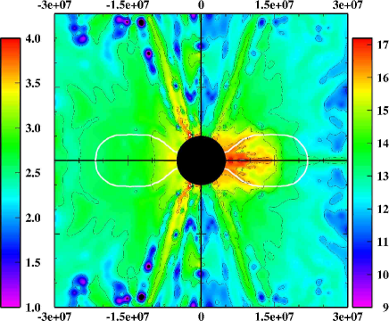
Figure 1: Logarithmic contour of differential rotation (:$Xd\Omega/dX$) (left) and amplification rate of toroidal magnetic field (:$dB_{\phi}/dt$) (right).

Figure 1 shows the differential rotation and amplification rates of toroidal magnetic field of model B9J1.5 at 7.99 s, just before the launch of the MHD outflows from the accretion disk. The density takes its maximum value at around 120 km in the equatorial plane (left panel), in which the poloidal fields are strong because the higher compression is achieved (right panel). The white solid line in the right panel indicates the surface positions of the accretion disk. So the amplifications of the poloidal fields occur most efficiently inside the accretion disk. It is noted here that the disk is gravitationally stable because the adiabatic index ($\gamma$) inside the disk becomes greater than $4/3$ due to the contribution of the non-relativistic nucleon ($\gamma=5/3$) photodissociated from the iron nuclei. Figure 1 shows that the amplification rates of toroidal magnetic field are highest also inside the disk (right), because the degree of the differential rotation is large there (left). In previous collapsar simulations assuming much larger angular momentum initially, it seems to be widely agreed that the differential rotation is a primary agent to amplify the toroidal fields. On the other hand, our results show that for long-term evolution of relatively slow rotation models, the amplification of the poloidal fields by compression is preconditioned for the amplification of the toroidal fields.

II.2.2 two types of megneto-driven outflow

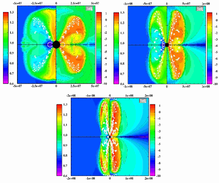
Figure 2: Evolution of MHD jets launched from the accretion disk (Type II jets). In each panel, logarithmic contour of entropy (left side) and the inverse of plasma beta (e.g., $\beta_{\rm mag}^{-1}\equiv B^{2}/8\pi/p$) (right side) are shown at 1.43 s (top left), 1.87 s (top right), and 2.11 s (bottom) for model B10J1.5. Note the difference of the length scales among panels.

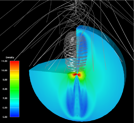
Figure 3: Three dimensional plot of density with the magnetic field lines (silver line) for B10J1.5 model near at the moment of the shock break-out (2.11 s). Color contour on the two-dimensional slice represents the logarithmic density.

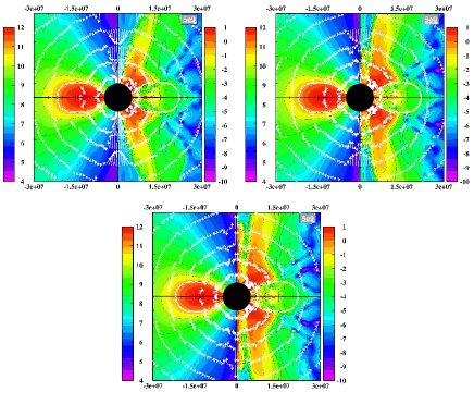
Figure 4: Same as Figure 2 but for model B9J1.5 at 8.115 s (top left), 8.148 s (top right), and 8.154 s (bottom), showing the moment of the formations of jets in type I.

Figure 2 shows the evolution of the MHD outflow for model B10J1.5, from its initiation near from the inner edge of the accretion disk (top left), propagation along the polar axis (top right), till they come out of the iron core (bottom). Note the difference of the length scales in each panel. Among the computed models, this model has the strongest initial magnetic fields with smallest angular momentum (e.g., Table 1). The toroidal fields can be much stronger than for other models, by the enhanced compression of the poloidal fields inside the disk. As a result, the MHD outflow is so strong that they do not stall, once they are launched. In fact, the outflow is shown to be kept magnetically-dominated (inverse of the plasma beta greater than 1, right-hand side in Figure 2) till the shock break-out. As the outflow propagates rather further from the center (top right), the outflow begins to be collimated due to the magnetic hoop stresses, and keep their shape till the shock-breakout (Figure 3).

We move to discuss the jets in type I, by taking model B9J1.5 as an example. In this case, the magnetic outflow from the accretion disk is not as strong as model B10J1.5, and stalls at first in the iron core (see butterfly-like regions colored by red in the top left panel (right-hand side) in Figure 4). In the top right panel, very narrow regions near along the rotational axis are seen to be produced in which the magnetic pressure dominate over the matter pressure (colored by red in the right-hand side). Such regions are formed by turbulent inflows of the accreting material from the equator, crossing the butterfly-like regions outside the disk, to the polar regions. Such flow-in materials obtain sufficient magnetic amplifications when they approach to the rotational axis where the differential rotation is stronger, leading to the formations of the MHD outflows along the rotational axis (bottom).

Now we proceed to look more in detail to the properties of the MHD jets. The jet of model B10J1.5 has the largest explosion energy with largest baryon loading. This is because the jet is type II as mentioned. Since the jet is launched rather earlier ($\sim 1.9s$) than for type I, there is much material near the rotational axis, which makes the baryon load of jets larger for the model. For type I jets, no systematic dependence of the initial angular momentum on the masses and the energies is found. We think that this is because the formation of the type I jets occurs by turbulent inflows as already mentioned in the previous section. The similarity between types I and II is that the jets are at most subrelativistic (0.07c for model B10J1.5) with the explosion energy less than $10^{49}\mathrm{erg}$. While the ordinary GRBs require the highly relativistic ejecta, we speculate that thesemildly relativistic ejecta may be favorable for X-ray flashes (XRF).

III Neutrino-Driven Jet from Collapsars

III.1 Numerical Method

III.1.1 neutrino pair annihilation in collapsars; ray-tracing method in special relativity

We develop a numerical scheme and code for estimating the energy and momentum transfer via neutrino pair annihilation ($\nu+{\bar{\nu}}\rightarrow e^{-}+e^{+}$), bearing in mind the application to the collapsar models of GRBs hari09b . To calculate the neutrino flux illuminated from the accretion disk, we perform a ray-tracing calculation in the framework of special relativity.

Figure 5 presents our calculation concept for the neutrino pair annihilation in collapsars (Figure 5). For estimating the neutrino pair annihilation at a given target, we trace each neutrino trajectory (white lines) backwards till it hits to the surface of the accretion disk (colored by red). We checked the accuracy of our code for various situations, and confirmed its validity.

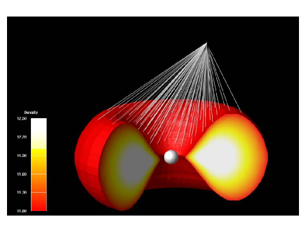
Figure 5: An example of the ray-tracing (white line) of neutrinos for estimating the neutrino pair annihilation towards a given point outside the accretion disk (indicated by red). The central sphere represents the black hole (BH).

III.1.2 two step simulation

In this section, we show results of the application of newly developed code for neutrino heating hari09b to collapsars. First of all, we note our basic strategy. Our numerical procedure is divided into two steps, STEP I and STEP II, depending on the inclusion of neutrino heating, since it is numerically expensive. In STEP I, we follow the evolution of collapsar from the onset of core-collapse without neutrino heating and evaluate the effect of neutrino heating in post-processing step. If the neutrino heating meets the condition for outflow formation, we go into STEP II in which we restart our simulation including neutrino heating from the time when the heating becomes important for dynamics. The criterion of this switching is whether $\tau_{\rm dyn}$ is greater than $\tau_{\rm heat}$ or not, where $\tau_{\rm dyn}$ and $\tau_{\rm heat}$ is the dynamical timescale of materials and the timescale for materials to escape from gravitational field by neutrino heating, respectively. Therefore, the condition $\tau_{\rm dyn}/\tau_{\rm heat}>1$ means that materials can escape from gravitational field by neutrino energy deposition. Here, the dynamical timescale is given by $\tau_{\rm dyn}\equiv\sqrt{3\pi/16G{\bar{\rho}}}$, where $G$ is the gravitational constant and ${\bar{\rho}}$ is average density derived from spherical mass coordinate $M(r)$ as ${\bar{\rho}}\equiv 3M(r)/4\pi r^{3}$. Heating time scale is given by $\tau_{\rm heat}\equiv\rho|\Phi_{\rm tot}|/q^{+}$, where $\rho$, $q^{+}$, and $\Phi_{\rm tot}$ is the density, the energy deposition rate by neutrino heating, and the total gravitational potential.

In STEP I, we start our simulation from the onset of core-collapse of the rotating massive star. The time-evolution is followed by special relativistic hydrodynamic code developed by taki09 ; hari09a . Since the massive star is thought to form the BH after the onset of core-collapse, we simply assume the formation of the BH by setting absorptive inner boundary, and put a point mass $M_{\rm BH}$ at the center of the progenitor.

In terms of heating, we include the energy deposition and the momentum transfer by neutrino-antineutrino pair annihilation for electron type neutrino. To calculate the heating rate, we adopt the method in hari09b , which is developed for the rapid calculation of pair annihilation in collapsars. With this method, we evaluate the heating rate in the post-processing step in STEP I. Since the simulation of heating is still time-demanding to couple with the hydrodynamics code, we calculate neutrino heating once in every 50 hydrodynamical steps in STEP II, which is enough to capture the dynamical change of the neutrino flux from the accretion disk.

We calculated 4 models with various profiles of rotation. Model name is given as ’JX’ representing the model with angular momentum $j=Yj_{\rm lso}$.

III.2 Result

III.2.1 when the neutrino heating becomes important ?

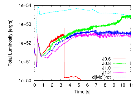
Figure 6: Time evolution of total luminosity and the mass accretion rate. Plots for the luminosity of J0.6 model (solid), J0.8 model (dashed), J1.0 model (dotted), J1.2 model (small dotted), and the mass accretion rate in J0.8 model (dot dashed) is shown.

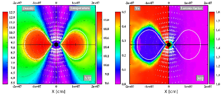
Figure 7: Hydrodynamic configuration when the accretion disk is in a stationary state (here, 9.1 s after the onset of core-collapse). In the left panel, the logarithmic density (in$\mathrm{g/cm^{3}}$, left-half) and temperature (in $K$, right-half) are shown. The right panel shows the electron fraction (left-half) and the Lorentz factor (right-half).

Model	Outflow	$L_{\nu}[{\rm erg\,\,s^{-1}}]$	$Q_{\nu{\bar{\nu}}}[{\rm erg\,\,s^{-1}}]$	${\dot{E}_{\rm exp}}[{\rm erg}]$
J0.6	No	$5.0\times 10^{50}$	$-$	$0.0$
J0.8	Yes	$1.2\times 10^{53}$	$3.1\times 10^{50}$	$4.0\times 10^{49}$
J1.0	No	$4.1\times 10^{52}$	$2.9\times 10^{49}$	$0.0$
J1.2	No	$2.3\times 10^{52}$	$8.9\times 10^{48}$	$0.0$

Table 2: Properties of our models. Contents of each cell is, whether the neutrino-driven outflows are formed (yes or no), the total neutrino luminosity $L_{\nu}$, the neutrino heating rate by pair annihilation $Q_{\nu{\bar{\nu}}}$, and the increasing rate of explosion energy ${\dot{E}_{\rm exp}}$.

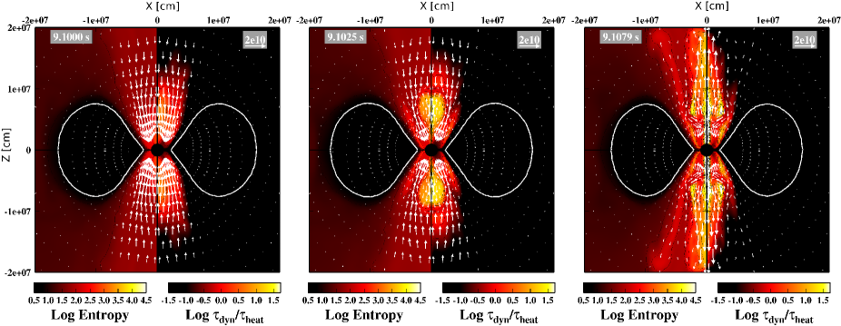
Figure 8: Relativistic outflow production in J0.8 model. In each panel, logarithmic contour of the entropy (left) and the ratio of the heating timescale to the dynamical timescale $\tau_{\rm dyn}/\tau_{\rm heat}$ (right) are drawn. Each panel corresponds to 9.1000 s (left), 9.1025 s (center), and 9.1079 s (right) after the onset of core-collapse, respectively. The white solid line denotes the area where the density is equal to $10^{11}\mathrm{g/cm^{3}}$, showing the surface of the accretion disk.

First of all, we mention about the evolution of collapsars without neutrino heating for 11 s (STEP I). All of our models initially collapse into the inner radius. When relatively rapidly rotating matter with, especially at the edge of Fe core, reaches near the inner radius, material crosses the equatorial plane and a shock is formed there ($\approx$ 0.8 s). This shock efficiently converts kinetic energy to thermal energy, then thick disk is formed in all models. At 2.0 s after the onset of core-collapse, $M_{\rm BH}$ becomes greater than 2 $M_{\odot}$ in each model, which would safely verify our assumption of BH formation. Figure 7 shows the stationary disk at 9.1 s after the onset of core-collapse in J0.8 model. We find that large and hot disk can be formed for models with angular momentum smaller than $j_{rmlso}$.

Here after we move to the effect of neutrinos emitted from the accretion disk. One of the most important ingredients for neutrino-driven outflow would be the total luminosity of neutrino, which will be potentially converted to the thermal energy. Figure 6 shows time evolution of the neutrino luminosity. We fine that after several seconds (namely 5 s), the neutrino luminosity can become greater than $10^{53}\rm ergs\,\,{s}^{-1}$. We also find that the criterion for outflow formation $\tau_{\rm dyn}/\tau_{\rm heat}>1$ is safely satisfied after about 9.0 s only in J0.8 model, indicating that outflow would be launched. Therefore we move onto STEP II and restart our simulation including neutrino heating from 9.0 s.

III.2.2 formation of neutrino-driven outflow

In STEP II, we find that just after we restart with neutrino heating, an outflow is launched from the polar funnel in J0.8 model, while not in other models. Table 2 shows the main results of this work. In this table, the total luminosity $L_{\rm tot}$, the total energy deposition rate $Q_{\nu{\bar{\nu}}}$ , and the luminosity of the explosion energy ${\dot{E}}_{\rm exp}$ of our models are shown, which are given by the average value from 9.1000 s till 9.2044 s after the onset of core-collapse. As shown, ${\dot{E}}_{\rm exp}$ is non-zero ($4.0\times 10^{49}\rm ergs\,\,{s}^{-1}$) only for J0.8 model. This outflow is driven by neutrino-antineutrino pair annihilation, which we will discuss below. Amang all models, J0.8 model has the largest luminosity $L_{\rm tot}\approx 1.2\times 10^{53}\rm ergs\,\,{s}^{-1}$ and energy deposition rate $Q_{\nu{\bar{\nu}}}\approx 3.1\times 10^{50}\rm ergs\,\,{s}^{-1}$, respectively, providing the energy conversion efficiency of 0.26 %. $Q_{\nu{\bar{\nu}}}$ is comparable to the artificial energy deposition rate in previous studies (e.g., macf99 ; aloy00 ), indicating the analogeous outcomes in the outer layer. We note that ${\dot{E}}_{\rm exp}$ of J0.8 model is consistent with typical energy of $\gamma$-ray in the rest frame of GRBs ($\approx 10^{51}\rm ergs\,\,{s}^{-1}$) if this outflow continues for about 100 s and the conversion rate to kinetic energy is several 10 % (e.g., frail01 ), indicating the connection between our model and GRBs.

IV Summary

We have performed a series of numerical simulation of collapsars from core-collapsing phase of massive star. We focus on indevestigating whether outflow can be launched by MHD and/or neutrino process. In terms of MHD process, we find that initial weak poloidal magnetic field is much amplified inside the disk by compression. Such strong magnetic field can amplify the toroidal magnetic field. We find that after several seconds, magnetic pressure dominates over the thermal pressure, and trigers the formation of outflow. We also find that there are two types of MHD outflows in long-term evolution from core-collapse. Although these outflows are weak $(\approx 10^{48}\rm ergs\,\,{s}^{-1})$, it can be candidate for the source of XRF.

As for the neutrino process, we developed numerical code for pair neutrino annihilation, and applied it to collapsars. We find that the condition for the outflow production by neutrino-antineutrino pair annihilation is fulfilled inside 100 km on the axis at 9 s after core-collapse. Including the energy deposition by neutrino, we find that neutrino-driven outflow is formed along the rotational axis. In addition, the outflow becomes relativistic. Such relativistic outflow can keep collimated till it penetrate the outer layer. These features suggests the connection between neutrino-driven outflows and GRBs.

- (1) Aloy, M. A., et al. 2000, ApJ, 531, L119
- (2) Birkl, R., Aloy, M. A., Janka, H.-T., & Müller, E. 2007, A&A, 463, 51
- (3) Fujimoto, S.-i., et al. 2006, ApJ, 644, 1040
- (4) Frail, D. A., et al. 2001, ApJ, 562, L55
- (5) Harikae, S., Takiwaki, T., & Kotake, K. 2009, ApJ, 704, 354
- (6) Harikae, S., Kotake, K., & Takiwaki, T. 2009, arXiv:0912.2590
- (7) Komissarov, S. S., & McKinney, J. C. 2007, MNRAS, 377, L49
- (8) MacFadyen, A. I. & Woosley, S. E. 1999, ApJ, 524, 262
- (9) McKinney, J. C., & Narayan, R. 2007, MNRAS, 375, 531
- (10) Mizuta, A., et al. 2006, ApJ, 651, 960
- (11) Nagataki, S., et al. 2007, ApJ, 659, 512
- (12) Nagataki, S. 2009, ApJ, 704, 937
- (13) Paczynski, B. 1998, ApJ, 494, L45
- (14) Proga, D., et al. 2003, ApJL, 599, L5
- (15) Takiwaki, T., Kotake, K., & Sato, K. 2009, ApJ, 691, 1360
- (16) Woosley, S. E. 1993, ApJ, 405, 273
- (17) Woosley, S. E. & Heger, A. 2006, ApJ, 637, 914