Domain walls with non-Abelian orientational moduli

Abstract

Domain walls with non-Abelian orientational moduli are constructed in $U(N)$ gauge theories coupled to Higgs scalar fields with degenerate masses. The associated global symmetry is broken by the domain walls, resulting in the Nambu-Goldstone (and quasi-Nambu-Goldstone) bosons, which form the non-Abelian orientational moduli. As walls separate, the wave functions of the non-Abelian orientational moduli spread between domain walls. By taking the limit of Higgs mass differences to vanish, we clarify the convertion of wall position moduli into the non-Abelian orientational moduli. The moduli space metric and its Kähler potential of the effective field theory on the domain walls are constructed. We consider two models: a $U(1)$ gauge theory with several charged Higgs fields, and a $U(N)$ gauge theory with $2N$ Higgs fields in the fundamental representation. More details are found in our paper[1].

1 BPS solitons

Solitons are useful to build unified models with extra dimensions, and to provide all or part of nonperturbative effects. If a global symmetry of the theory is spontaneously broken by the presence of solitons, Nambu-Goldstone (NG) bosons come out and form (a part of) the moduli space of the soliton. In the case of non-Abelian global symmetry, the resulting massless modes can have non-Abelian orientational moduli. Quite often solitons have parameters, which are called moduli. If we promote these parameters to fields on the world volume of the soliton, they become massless fields in the low-energy effective field theory on the soliton.

Simplest of solitons is the domain wall which depends only on one spatial dimension, namely co-dimension one soliton. In order to have a domain wall, we need to have discrete vacua. As the simplest theory with two discrete degenerate vacua, let us consider a $1+1$ dimensional theory of real scalar field $\varphi$ with a double well potential

$${\cal L}=\partial_{\mu}\varphi\partial^{\mu}\varphi-\lambda(\varphi^{2}-v^{2})^{2},\qquad\lambda>0.$$ (1)

If there is a field configuration connecting the two discrete degenerate vacua, $\varphi_{+}\equiv v$ and $\varphi_{-}\equiv-v$, we obtain a domain wall separating two vacua, as a kink, whose energy density is localized, resulting in the domain wall. The nontrivial boundary condition at infinity assures the topological stability of the configuration: topological charge is characterized by $\pi_{0}({\cal M})$. To obtain such a solution, let us assume a static configuration depending only on one spatial direction $y$, and form the following complete square of the energy density

$${\cal E} = (\partial_{y}\varphi)^{2}+\lambda(\varphi^{2}-v^{2})^{2}$$ (2)

$$= (\partial_{y}\varphi+\sqrt{\lambda}(\varphi^{2}-v^{2}))^{2}+\partial_{y}\left[2\sqrt{\lambda}\left(v^{2}\varphi-{\varphi^{3}\over 3}\right)\right].$$

This is called the Bogomol’nyi completion giving the lower bound of energy which is called the Bogomol’nyi bound

$$\int_{-\infty}^{\infty}dy{\cal E}\geq\left[2\sqrt{\lambda}\left(v^{2}\varphi-{\varphi^{3}\over 3}\right)\right]_{-\infty}^{\infty}.$$ (3)

The Bogomol’nyi bound is saturated if and only if the following first order differential equation is satisfied:

$$\partial_{y}\varphi+\sqrt{\lambda}(\varphi^{2}-v^{2})=0,$$ (4)

which is called the Bogomol’nyi-Prasad-Sommerfield (BPS) equation for the domain wall. The BPS equation is easily solved to give the BPS domain wall solution

$$\varphi=v\tanh(\sqrt{\lambda}v(y-y_{0})).$$ (5)

The BPS domain wall solution has a single modulus $y_{0}$, whose physical meaning is the position of the wall. This modulus can also be understood as a NG mode corresponding to the spontaneously broken translational symmetry. We can promote the real scalar to complex scalar, and add a fermion with appropriate interactions to make the system supersymmetric. Namely we can embed the theory (1) into a supersymmetric theory with four supercharges. The BPS solution preserves the half of the supersymmetry in this embeded theory. This is a typical example of the BPS solitons which can be understood as the BPS state preserving a part of the supersymmetry in a supersymmetric theory.

As another example of solitons, we can consider vortex in a theory with the Abelian gauge field $W_{\mu}$ coupled to a charged complex scalar field $\phi$

$${\cal L}=-\frac{1}{4e^{2}}F_{\mu\nu}F^{\mu\nu}+{\cal D}^{\mu}\phi({\cal D}_{\mu}\phi)^{\dagger}-\frac{\lambda}{4}\left(\phi\phi^{\dagger}-v^{2}\right)^{2},$$ (6)

where ${\cal D}_{\mu}\phi=(\partial_{\mu}+iW_{\mu})\phi$ denotes the covariant derivative, and $F_{\mu\nu}=\partial_{\mu}W_{\nu}-\partial_{\nu}W_{\mu}$ the field strength. The mapping from the infinity in the $x,y$ plane ($S^{1}$) to the vacuum manifold $|\phi|=v,S^{1}$ gives a topological charge $\pi_{1}(S^{1})$ assuring the stability of the vortex configuration.

$$k=-{1\over 2\pi}\int d^{2}x\ F_{12}$$ (7)

The position of a single vortex is again a modulus, since the vortex can be formed anywhere in the $x,y$ plane. If there are two or more vortices, the gauge field induces repulsive force between the vortices, and the scalar field induces attractive interactions. When $e^{2}=\lambda$, the two interactions cancel each other and there is no static force between vortices. Therefore vortices can be placed at anywhere relative to each other, and the relative positions become additional moduli. This critical case corresponds precisely to the case where the theory can be embedded into supersymmetric theory by adding fermions appropriately. The vortex solutions can then be understood as the BPS solitons preserving the half of the supersymmetry. If there are internal global symmetry which are broken by the presence of solitons, the NG modes emerge. In particular, if the global symmetry is non-Abelian, we can have non-Abelian orientational moduli for the soliton. These non-Abelian orientational moduli exhibits interesting properties similar to the D-branes in string theory.

2 BPS equations for $U(N)$ gauge theories and the moduli matrix

We consider $U(N_{\rm C})$ gauge theory in space-time dimension $d=4+1$ with a real scalar field $\Sigma$ in the adjoint representation and $N_{\rm F}\,(>N_{\rm C})$ flavors of massive Higgs scalar fields in the fundamental representation, denoted as an $N_{\rm C}\times N_{\rm F}$ matrix $H$. Choosing the minimal kinetic term, we obtain

$${\cal L} = {\cal L}_{\rm kin}-V,$$ (8)

$${\cal L}_{\rm kin} = {\rm Tr}\left(-{1\over 2g^{2}}F_{\mu\nu}F^{\mu\nu}+\frac{1}{g^{2}}{\cal D}_{\mu}\Sigma\,{\cal D}^{\mu}\Sigma+{\cal D}^{\mu}H\left({\cal D}_{\mu}H\right)^{\dagger}\right),$$ (9)

where the covariant derivatives and field strengths are defined as ${\cal D}_{\mu}\Sigma=\partial_{\mu}\Sigma+i[W_{\mu},\Sigma]$,   ${\cal D}_{\mu}H=(\partial_{\mu}+iW_{\mu})H$,   $F_{\mu\nu}=-i[{\cal D}_{\mu},\,{\cal D}_{\nu}]$. Our convention for the space-time metric is $\eta_{\mu\nu}={\rm diag}(+,-,\cdots,-)$. The scalar potential $V$ is given in terms of a diagonal mass matrix $M$ and a real parameter $c$ as

$$V = {\rm Tr}\Big{[}\frac{g^{2}}{4}\left(c\mathbf{1}-HH^{\dagger}\right)^{2}+(\Sigma H-HM)(\Sigma H-HM)^{\dagger}\Big{]}.$$ (10)

The 1/2 BPS equations for domain walls interpolating the discrete vacua can be obtained by usual Bogomol’nyi completion of the energy

$$E = \int_{-\infty}^{\infty}dy\,{\rm Tr}\left[(\mathcal{D}_{y}H-HM+\Sigma H)^{2}+\frac{1}{g^{2}}\left({\cal D}_{y}\Sigma-\frac{g^{2}}{2}\left(c{\bf 1}-HH^{\dagger}\right)\right)^{2}+c\,{\cal D}_{y}\Sigma\right]$$ (11)

$$\geq c\Big{[}{\rm Tr}\,\Sigma(\infty)-{\rm Tr}\,\Sigma(-\infty)\Big{]}.$$ (12)

The first order differential equations for the configurations saturating this energy bound are of the form [7]

$$\mathcal{D}_{y}H=HM-\Sigma H,\qquad\mathcal{D}_{y}\Sigma=\frac{g^{2}}{2}\left(c{\bf 1}-HH^{\dagger}\right).$$ (13)

Here we consider static configurations depending only on the $y$-direction.

Let us solve these 1/2 BPS equations. Firstly the first equation can be solved by [7]

$$H=S^{-1}(y)H_{0}e^{My},\quad\Sigma+iW_{y}=S^{-1}(y)\partial_{y}S(y).$$ (14)

Here $H_{0}$, called the moduli matrix, is an $N_{\rm C}\times N_{\rm F}$ constant complex matrix of rank $N_{\rm C}$, and contains all the moduli parameters of solutions. The matrix valued quantity $S(y)\in GL(N_{\rm C},{\bf C})$ is determined by the second equation in (13) which can be converted to the following equation for $\Omega\equiv SS^{\dagger}$:

$$\frac{1}{cg^{2}}\bigl{[}\partial_{y}(\Omega^{-1}\partial_{y}\Omega)\bigl{]}={\bf 1}_{N_{\rm C}}-\Omega^{-1}\Omega_{0},\hskip 28.45274pt\Omega_{0}\equiv\frac{1}{c}H_{0}e^{2My}H_{0}^{\dagger}.$$ (15)

This equation is called the master equation for domain walls. From the vacuum conditions at spatial infinities $y\rightarrow\pm\infty$, we can see that the solution $\Omega$ of the master equation should satisfy the boundary condition $\Omega\rightarrow\Omega_{0}$ as $y\rightarrow\pm\infty$. It determines $S$ for a given moduli matrix $H_{0}$ up to the gauge transformations $S^{-1}\rightarrow US^{-1},~{}U\in U(N_{\rm C})$ and then the physical fields can be obtained through (14). Note that the master equation is symmetric under the following $V$-transformations

$$H_{0}\rightarrow VH_{0}\quad{\rm and}\quad S(y)\rightarrow VS(y)\quad{\rm with}\quad V\in GL(N_{\rm C},{\bf C}),$$ (16)

and if the moduli matrices are related by the $V$-transformations $H_{0}^{\prime}=VH_{0}$, they give physically equivalent configurations. We call this equivalence relation as the $V$-equivalence relation and denote it as $H_{0}\sim VH_{0}$. The solution of the master equation exists and unique for any given $H_{0}$ at least for the $U(1)$ gauge theory [5]. For $U(N)$ gauge theory the number of moduli parameters agrees with the the result of index theorem [6].

3 Non-Abelian orientational moduli of walls in a $U(1)$ gauge theory

So far, domain walls with eight supercharges have been mostly considered in gauge theories with $U(1)$ gauge field [2]–[5], $U(1)\times U(1)$ gauge field [11], or $U(N)$ gauge fields [7]–[10] coupled to Higgs scalar fields with non-degenerate masses except for [12, 13]. In the case of non-degenerate Higgs masses, the flavor symmetry is Abelian: $U(1)^{N_{\rm F}-1}$ and the symmetry of the vacua is also Abelian. As a result each domain wall carries a $U(1)$ orientational modulus [2, 7]; The moduli space of a single domain wall is

$${\cal W}^{k=1}\simeq{\bf R}\times S^{1}.$$ (17)

From this viewpoint, these domain walls should be called Abelian domain walls even when the gauge symmetry of the Lagrangian is non-Abelian [7]–[11].

Let us see the non-Abelian orientational moduli in a simple example of the Abelian gauge theory coupled with the $N_{\rm F}=4$ Higgs fields.

3.1 Vacua of the $U(1)$ gauge theory

The massless vacuum manifold is $T^{\star}{\bf C}P^{3}$ where the base manifold is parametrized by

$${\bf C}P^{3}=\left\{HH^{\dagger}=c\right\}/U(1),\quad H=\sqrt{c}\left(h_{1},\ h_{2},\ h_{3},\ h_{4}\right),$$ (18)

where the quotient is the overall $U(1)$. The vacuum manifold is expressed as (the inside and the surface of) a triangular pyramid in the 3 dimensional space $(|h_{1}|^{2},|h_{2}|^{2},|h_{3}|^{3})$, as shown in Fig. 1 (c). When the mass matrix containing a small parameter $\epsilon$ ($0\leq\epsilon\in{\bf R}$)

$$M={\rm diag}\left(m,\ \frac{m\epsilon}{2},\ -\frac{m\epsilon}{2},\ -m\right)$$ (19)

is turned on, the vacuum manifold is lifted except for four points and the flavor symmetry breaks from $SU(4)$ to $U(1)^{3}$. These discrete vacua are the four vertices of the pyramid shown in Fig. 1 (a). We label those vacua as $\left<A\right>$ $(A=1,2,3,4)$. The vacuum expectation value (VEV) of the vacuum $\left<A\right>$ is $h_{B}=\delta_{AB}$. Taking a limit of $\epsilon\to 0$, the second and the third Higgs fields become degenerate so that the flavor symmetry enhances from $U(1)^{3}$ to $U(1)^{2}\times SU(2)\in SU(4)$.

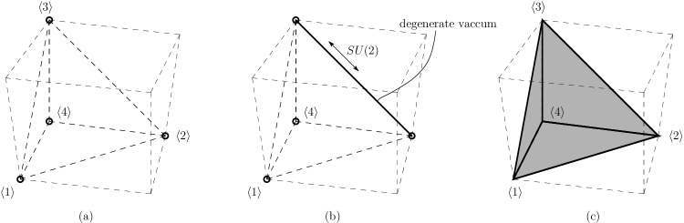
Figure 1: Vacua for various cases of mass configurations plotted in the three-dimensional space of Higgs fields $h_{i}^{2},i=1,2,3$ with $\sum_{i=1}^{4}h_{i}^{2}=1$. (a) non-degenerate massive vacua (b) massive degenerate and non-degenerate vacua (c) massless vacuum.

There are two isolated vacua and one degenerate vacuum ${\bf C}P^{1}\simeq SU(2)/U(1)$ represented by a line connecting $\left<2\right>$ and $\left<3\right>$ as shown by a thick line in Fig.1(b). We denote this degenerate vacuum as $\left<\hbox{2-3}\right>$.

3.2 Domain walls in the $U(1)$ gauge theory

There exist domain wall solutions interpolating vacua in the model with fully or partially non-degenerate Higgs masses. In the case of $N_{\rm C}=1$, the moduli matrix and the $V$-equivalence (16) take the form of

$$H_{0}=\left(\phi_{1},\ \phi_{2},\ \phi_{3},\ \phi_{4}\right)\sim\lambda\left(\phi_{1},\ \phi_{2},\ \phi_{3},\ \phi_{4}\right),\quad\lambda\in{\bf C}^{*}.$$ (20)

In terms of the moduli matrix the vacua $\left<A\right>$ are described by $\phi_{B}=\delta_{BA}$ for $B=1,2,3,4$. Since we want to consider the domain wall interpolating the vacua $\left<1\right>$ and $\left<4\right>$ (passing by $\left<2\right>,\left<3\right>$ on the way), the parameter $\phi_{1}$ and $\phi_{4}$ should not be zero while $\phi_{2},\phi_{3}$ can become zero. So the moduli space corresponding to the multiple domain walls which connect $\left<1\right>$ and $\left<4\right>$ is

$${\cal M}\simeq\left({\bf C}^{2}\times({\bf C}^{*})^{2}\right)//{\bf C}^{*}\simeq{\bf C}^{*}\times{\bf C}^{2},$$ (21)

where double slash denotes identification by the $V$-transformation. Here the part ${\bf C}^{*}\simeq{\bf R}\times U(1)$ represents the translational modulus and the associated phase modulus.

When we take the gauge coupling $g$ to infinity, the model reduces to a nonlinear sigma model whose target space is the Higgs branch of the vacua $T^{*}{\bf C}P^{3}$ in the original theory. To make the discussion simple, we take this limit for a while. One benefit to consider the nonlinear sigma model is that the BPS equations can be analytically solved. In fact the solutions are expressed as [8]

$$H=\frac{1}{\sqrt{\Omega}_{0}}H_{0}e^{My}\quad{\rm with}\quad\Omega_{0}\equiv H_{0}e^{2My}H_{0}^{\dagger}.$$ (22)

A domain wall solution corresponds to a trajectory connecting the vertex $\left<1\right>$ and $\left<4\right>$. Flows from $\left<1\right>$ to $\left<4\right>$ inside the pyramid are shown in Fig. 2.

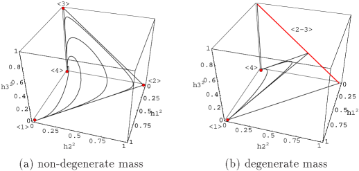
Figure 2: Domain wall trajectories in the target space ${\bf C}P^{3}$ for non-degenerate mass (a) and for degenerate mass (b).

Physical meaning of the moduli parameters becomes much clearer by using the $V$-equivalence relation (20) to fix the form of the moduli matrix as

$$H_{0}=\left(1,\ e^{\varphi_{1}},\ e^{\varphi_{1}+\varphi_{2}},\ e^{\varphi_{1}+\varphi_{2}+\varphi_{3}}\right).$$ (23)

Furthermore, one may be visually able to see the “kink” configuration in the profile of the field $\Sigma=(1/2)\partial_{y}\log\Omega_{0}$. In the vacuum region $\left<A\right>$ the function $\Sigma(y)$ takes the value $\Sigma=m_{A}$. Several solutions are shown in Fig. 3.

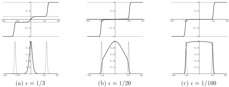
Figure 3: Configuration of $\Sigma$ (first row) and density of the Kähler metric of $\varphi_{1}$, $\varphi_{2}$ and $\varphi_{3}$ (second row). Moduli parameters are $(\varphi_{1},\varphi_{2},\varphi_{3})=(20,0,-20)$ and $m=1$.

The domain wall positions can be roughly read from the moduli matrix in Eq. (23) as

$$\frac{y_{+}}{L_{+}}=\varphi_{1}+\varphi_{1}^{*},\quad\frac{y_{0}}{L_{0}}=\varphi_{2}+\varphi_{2}^{*},\quad\frac{y_{-}}{L_{-}}=\varphi_{3}+\varphi_{3}^{*},$$ (24)

where $y_{+}$ is the position of the right wall and $y_{0},y_{-}$ are the positions for the middle and the left walls, respectively. Here $L_{\pm,0}$ stands for the width of each wall

$$L_{+}\equiv\frac{2}{m(2-\epsilon)},\quad L_{0}\equiv\frac{1}{m\epsilon},\quad L_{-}\equiv\frac{2}{m(2-\epsilon)}.$$ (25)

This rough estimation is, of course, valid only for well separated walls whose positions are aligned as $y_{-}\ll y_{0}\ll y_{+}$, see Fig. 3 (a). Each domain wall is accompanied by a complex moduli parameter $\varphi_{i}$ whose real part is related to the wall position and imaginary part is the $U(1)$ internal symmetry (the NG mode associated with the broken $U(1)$ flavor symmetry).

To argue symmetry aspects of the moduli parameters, first let us consider a model which has completely non-degenerate masses and domain walls interpolating between those vacua. The global symmetry explicitly breaks from $SU(4)$ to $U(1)^{3}\subset SU(4)$. We take, as the unbroken global symmetries, $U_{1}(1),U_{2}(1)$ and $U_{3}(1)$ with generators ${\rm diag}\left(1,-1,-1,1\right)$, ${\rm diag}\left(1,0,0,-1\right)$, and ${\rm diag}\left(0,1,-1,0\right)$ respectively. Each vacuum $\left<A\right>$ preserves all of these symmetries. However, once domain walls connecting those vacua appear, they break all or a part of these symmetries. For example, the moduli matrix $H_{0}=(1,0,0,\phi_{4})$ corresponding to a domain wall connecting two vacua $\left<1\right>$ and $\left<4\right>$ breaks $U_{2}(1)$ but still preserves $U_{1}(1)$ and $U_{3}(1)$. Here note that overall phase can be absorbed by the $V$-transformation (20). Therefore the phase of the moduli parameter $\phi_{4}$ corresponds to nothing but the broken global symmetry $U_{2}(1)$. This implies the NG mode localizes around the domain wall as we saw above. For the moduli matrix $H_{0}=(1,\phi_{2},0,\phi_{4})$, which corresponds to two domain walls connecting three vacua $\left<1\right>\to\left<2\right>\to\left<4\right>$, the symmetry $U_{3}(1)$ in addition to $U_{2}(1)$ breaks while a combination of $U_{1}(1)$ and $U_{3}(1)$ is still preserved. Moreover, when we turn on the third element in the moduli matrix as $H_{0}=(1,\phi_{2},\phi_{3},\phi_{4})$, the third vacuum region appears and then the configuration has three domain walls connecting four vacua $\left<1\right>\to\left<2\right>\to\left<3\right>\to\left<4\right>$. In this case all of $U(1)^{3}$ are broken by the domain walls, so that corresponding three NG modes appear. These three NG modes are described by imaginary parts of $\log\phi$, which are combined with the three positions (24), to form three complex coordinates of the moduli space ${\bf C}^{2}\times{\bf C}^{*}$.

Next we consider a limit where the second and the third masses are degenerate ($\epsilon\to 0$ in the mass matrix (19)). In the limit the global symmetry $U_{1}(1)\times U_{2}(1)\times U_{3}(1)$ is enhanced to $U_{1}(1)\times U_{2}(1)\times SU(2)$. At the same time, the degenerate vacuum $\left<\hbox{2-3}\right>$ appear instead of the two isolated vacua $\left<2\right>$ and $\left<3\right>$ as shown in Fig. 1 (b). At the degenerate vacuum, $U_{1}(1),U_{2}(1)$ are preserved but $SU(2)$ is broken to $U_{3}(1)$. Therefore the degenerate vacuum $\left<2{\rm-}3\right>$ is $SU(2)/U_{3}(1)={\bf C}P^{1}$. Non-vanishing $\phi_{4}\not=0$ causes the wall interpolating two vacua $\left<1\right>\to\left<4\right>$ and breaks only $U_{2}(1)$ again. Once the degenerate vacuum appears in the configuration such as two domain walls connecting vacua like $\left<1\right>\to\left<2{\rm-}3\right>\to\left<4\right>$, the breaking pattern of the global symmetry becomes different from that in the case of fully non-degenerate masses. The moduli matrix $H_{0}=(1,\phi_{2},\phi_{3},\phi_{4})$ describes such domain walls. Note that the second and the third elements break $SU(2)$ completely. The global symmetry $U_{1}(1)\times U_{2}(1)\times SU(2)$ are broken to $U(1)$ which is a mixture of $U_{1}(1)$ and $H\in SU(2)$. Emergence of the second wall and further $U(1)$-symmetry breaking are related to the facts that $|\phi_{2}|^{2}+|\phi_{3}|^{2}\not=0$ and $\phi_{4}\not=0$. These facts imply that the modes corresponding to the two broken $U(1)$’s localize around the walls accompanied by the two position moduli and the mode corresponding to $SU(2)/H$ have support in a region around the degenerate vacuum $\left<2{\rm-}3\right>$. We can count the number of the moduli parameters as follows. Two real parameters $\{|\phi_{2}|^{2}+|\phi_{3}|^{2},|\phi_{4}|^{2}\}$ correspond to the positions of the two walls whereas remaining four parameters correspond to the broken global symmetry $U_{1}(1)\times U_{2}(1)\times SU(2)/U(1)$. This is again consistent with ${\rm dim}_{{\bf R}}\left({\bf C}^{2}\times{\bf C}^{*}\right)$.

In the Fig. 3 we showed domain wall configurations of the three domain walls connecting the four vacua. As the parameter $\epsilon$ decreases, the width of the middle domain wall connecting the vacua $\left<2\right>$ and $\left<3\right>$ becomes broad and the tension of the wall becomes small since they are proportional to $1/\epsilon$ and $\epsilon$, respectively. When the width of the middle wall becomes larger than the separation of two outside walls, $L_{0}>y_{+}-y_{-}$, we can no longer see the middle wall. The density of the Kähler metric for the moduli parameters $\varphi_{1}$, $\varphi_{2}$ and $\varphi_{3}$ in the strong gauge coupling limit are shown in the second row of Fig. 3. The Kähler potential in the strong coupling limit is given by $K=c\int dy\ \log\Omega_{0}$ [14]. When three walls are well isolated as Fig. 3 (a), three modes corresponding to the moduli parameters $\varphi_{1}$, $\varphi_{2}$ and $\varphi_{3}$ are localized on the respective domain walls. As $\epsilon$ decreases, the density of the Kähler metric of $\varphi_{2}$ is no longer localized but is stretched between two outside domain walls. In the limit where $\epsilon\to 0$ the physical meaning of $\varphi_{2}$ as the position and the internal phase associated with the middle domain wall should be completely discarded. Instead, $\varphi_{2}$ gives the non-Abelian orientational moduli which comes from the ${\bf C}P^{1}$ zero modes of the degenerate vacua $\left<2{\rm-}3\right>$. For fixed moduli parameters $\varphi_{1},\varphi_{2},\varphi_{3}$, the domain wall solution as a function of $y$ sweeps out a trajectory in the target space ${\bf C}P^{3}$. These domain wall trajectories are shown for various values of moduli parameters in Fig. 2: the non-degenerate mass case (a) and the degenerate mass case (b). For the degenerate mass case, the trajectories do not go out from the triangular plane whose vertices are $\left<1\right>,\left<4\right>$ and one point on the edge between $\left<2\right>$ and $\left<3\right>$.

4 The Generalized Shifman-Yung (GSY) Model

4.1 $U(N)$ gauge theory

Let us now consider non-Abelian gauge theory with degenerate masses of the Higgs fields. Previously considered model is the $U(2)$ gauge theory with four Higgs fields in the fundamental representation with the mass matrix $M={\rm diag}(m,m,-m,-m)$ [12, 13], which we call the Shifman-Yung Model. The model enjoys a flavor symmetry $SU(2)_{\rm L}\times SU(2)_{\rm R}\times U(1)_{\rm A}$. It has been demonstrated that the coincident domain wall configurations break the flavor symmetry to $SU(2)_{\rm V}$ and the NG bosons corresponding to $[SU(2)_{\rm L}\times SU(2)_{\rm R}\times U(1)_{\rm A}]/SU(2)_{\rm V}\simeq U(2)$ appear in the effective action on the walls.

By generalizing the Shifman-Yung model, we consider the $U(N)$ gauge theory with $N_{\rm F}=2N$ Higgs fields in the fundamental representation whose mass matrix is given by

$$M~{}=~{}m{\sigma_{3}\over 2}\otimes{\bf 1}_{N}~{}=~{}{1\over 2}{\rm diag}(\overbrace{m,\cdots,m}^{N},\overbrace{-m,\cdots,-m}^{N}).$$ (26)

This system has a non-Abelian flavor symmetry $SU(N)_{\rm L}\times SU(N)_{\rm R}\times U(1)_{\rm A}$. Since we have only two mass parameters $m$ and $-m$, possible vacua are classified by an integer $0\leq k\leq N$: in the $k$-th vacua, there is a configuration in which $k$ flavors of the first half and $N-k$ flavors of the latter half take non-vanishing values and then $\Sigma$ and $H$ are

$$\Sigma\big{|}_{\rm vacuum} = {1\over 2}\,{\rm diag}(\overbrace{m,\cdots,m}^{k},\overbrace{-m,\cdots,-m}^{N-k}),$$

$$H\big{|}_{\rm vacuum} = \sqrt{c}\left(\begin{array}[]{cccc}{\bf 1}_{k}&{\bf 0}&{\bf 0}_{k}&{\bf 0}\\ {\bf 0}&{\bf 0}_{N-k}&{\bf 0}&{\bf 1}_{N-k}\end{array}\right).$$ (29)

This vacuum is labeled as $(k,N-k)$. The flavor symmetry $SU(N)_{\rm L}$ is broken down to $SU(k)_{\rm C+L}\times SU(N-k)_{\rm L}\times U(1)_{\rm C+L}$, and $SU(N)_{\rm R}$ is broken down to $SU(k)_{\rm R}\times SU(N-k)_{\rm C+R}\times U(1)_{\rm C+R}$, where $C+L,C+R$ denote the locking of the $L,R$ flavor symmetry with the $U(N)_{\rm C}$ color symmetry. Consequently the number of the discrete components of the vacua is $N+1$ in this system. Therefore in this vacua there emerge $4k(N-k)$ NG modes, which parametrize the direct product of two Grassmann manifolds,

$$G^{\rm L}_{N,k}\times G^{\rm R}_{N,k}.$$ (30)

Walls are obtained by interpolating between a vacuum at $y=-\infty$ and another vacuum at $y=\infty$. The boundary conditions at both infinities define topological sectors. For a given topological sector, we may find several walls. The maximal number of walls in this system is $N$, which are obtained for the following maximal topological sector

$$H=\left\{\begin{array}[]{cc}\sqrt{c}({\bf 1}_{N},{\bf 0}_{N})&{\rm at~{}}y=+\infty\\ \sqrt{c}({\bf 0}_{N},{\bf 1}_{N})&{\rm at~{}}y=-\infty\\ \end{array}\right..$$ (33)

The unbroken symmetries of the vacua $(N,0)$ and $(0,N)$ which we consider as the boundary condition of domain walls here, are $SU(N)_{\rm C+L}\times U(1)_{\rm C+L}\times SU(N)_{\rm R}$ and $SU(N)_{\rm L}\times SU(N)_{\rm C+R}\times U(1)_{\rm C+R}$, respectively. In this case, the moduli matrix $H_{0}$ can be set into the following form without loss of generality:

$$H_{0}=\sqrt{c}({\bf 1}_{N},e^{\phi})\sim\sqrt{c}(e^{-\phi},\,{\bf 1}_{N}),$$ (34)

where $e^{\phi}$ is an element of $GL(N,{\bf C})$ and $\phi$ describes the moduli space of walls of this system, and the two forms are related by the $V$-transformation (16). Therefore the moduli space of domain walls in the GSY model is

$${\cal M}\simeq GL(N,{\bf C})[=U(N)^{\bf C}]\simeq\left[{\bf C}^{*}\times SL(N,{\bf C})\right]/Z_{N}.$$ (35)

This moduli space admits the isometry

$$e^{\phi}\to e^{i\alpha}g_{\rm L}e^{\phi}g_{\rm R}^{\dagger}$$ (36)

with $(g_{\rm L},g_{\rm R})\in SU(N)_{\rm L}\times SU(N)_{\rm R}$ and $e^{i\alpha}\in U(1)_{\rm A}$. This is because the domain wall solutions break the symmetry of the two vacua $(N,0)$ and $(0,N)$, $G=SU(N)_{\rm C+L}\times SU(N)_{\rm C+R}\times U(1)_{\rm C+L-R}$, down to its subgroup.

4.2 Nambu-Goldstone (NG) modes and quasi-NG modes

Note the fact that the global symmetry $G=SU(N)_{\rm L}\times SU(N)_{\rm R}\times U(1)_{\rm A}$ in (36) acts on the moduli space metric as an isometry whereas the complexified group $G^{\bf C}=SL(N,{\bf C})_{\rm L}\times SL(N,{\bf C})_{\rm R}\times{\bf C}^{*}$ acts on it transitively but not as an isometry. Therefore $G^{\bf C}$ action may change the point in moduli space to another with a different symmetry structure. Since the symmetry of Lagrangian is $G$ but not $G^{\bf C}$ we can use only $G$ when we discuss the symmetry structure at each point in moduli space. General $\phi$ can be transformed by $G$ to

$$e^{\phi}={\rm diag.}(v_{1},v_{2},\cdots,v_{N})$$ (37)

with $v_{i}$ real parameters. When all $v_{i}$’s coincide (coincident walls), the unbroken symmetry is the maximal $H_{\rm max}=SU(N)_{\rm V}$, so we call it the symmetric point. There are $N^{2}$ massless NG bosons and $N^{2}$ quasi-NG bosons. When all $v_{i}$’s are different from each other (separated walls), $H_{\rm max}=SU(N)_{\rm V}$ is further broken down to $H_{\rm min}=U(1)_{\rm V}^{N-1}$. Here the numbers of NG bosons and quasi-NG bosons are $2N^{2}-(N-1)$ and $N-1$, respectively. These $N-1$ quasi-NG bosons correspond to the $N-1$ parameters $v_{i}$ without the overall factor. Therefore some of quasi-NG bosons at the symmetric point in the moduli space change to the NG bosons parametrizing $H_{\rm max}/H_{\rm min}=SU(N)_{\rm V}/U(1)_{\rm V}^{N-1}$ reflecting this further symmetry breaking. When some $v_{i}$’s coincide, some non-Abelian groups are recovered: $H=U(1)_{\rm V}^{r}\times\prod U(n_{i})_{\rm V}$. Then the NG modes $H_{\rm max}/H$ are supplied from quasi-NG modes.

The diagonal moduli parameters $v_{i}$ (quasi-NG bosons) in Eq. (37) correspond to the positions of $N$ domain walls. When all domain walls are separated, the unbroken symmetry is $U(1)_{\rm V}^{N-1}$. When positions of $n$ domain walls coincide, $U(n)_{\rm V}$ symmetry is recovered. This phenomenon has a resemblance to the case of D-branes. However, there is a crucial difference: the symmetry in our case of domain walls is a global symmetry, whereas that of D-branes is a local gauge symmetry. However in the case of the $d=2+1$ wall world-volume, massless scalars can be dualized to gauge fields. Shifman and Yung [12] expected that the off-diagonal gauge bosons of $U(N)$ (which are originally the off-diagonal NG bosons of $U(N)$ before taking a duality) will become massive when domain walls are separated, in order to interpret domain walls as D-branes. However, our analysis shows that the off-diagonal NG bosons of $U(N)$ remain massless, and instead some of the quasi-NG bosons become NG bosons for further symmetry breaking with the total number of massless bosons unchanged as explained.

We have obtained the low-energy effective Lagrangian explicitly for this model. We found the following. The wave functions of the NG boson for translation, for $U(1)^{N}$, and quasi-NG bosons are localized, and that other massless modes are extended between two domain walls, if walls are separated. Wave functions of all the massless modes become identical in the limit of coincident walls. These behaviors are different from D-branes, although there are some similarlities. More precise details of our results can be found in Ref.[1].

When we introduce complex masses for Higgs fields, domain wall junction or network emerge as $1/4$ BPS states [15]-[17]. In this case too, non-Abelain NG modes appear in the effective action, when some masses are degenerate [18], [19].

This work is supported in part by Grant-in-Aid for Scientific Research from the Ministry of Education, Culture, Sports, Science and Technology, Japan No.21540279, No.21244036 (N.S.).

Appendix

We will briefly give the derivation of our master equation (15). Let us first note an identity for variations $\delta_{i},i=1,2$ of arbitary regular matrix $A$

$$\delta_{1}(A^{-1}\delta_{2}A) = A^{-1}\delta_{1}\delta_{2}A-A^{-1}\delta_{1}AA^{-1}\delta_{2}A=A^{-1}(\delta_{2}\delta_{1}AA^{-1}-\delta_{1}AA^{-1}\delta_{2}AA^{-1})A$$ (38)

$$= A^{-1}\delta_{2}(\delta_{1}AA^{-1})A$$

For gauge invariant quantity $\Omega=SS^{\dagger}$, we obtain

$$\delta_{1}(\Omega\delta_{2}\Omega^{-1})=\delta_{1}(SS^{\dagger}\delta_{2}(S^{-1\dagger}S^{-1}))=\delta_{1}(SS^{\dagger}(\delta_{2}S^{-1\dagger})S^{-1}+S\delta_{2}S^{-1})$$

$$=S\left(\delta_{1}(S^{\dagger}\delta_{2}S^{-1\dagger})+S^{-1}\delta_{1}SS^{\dagger}\delta_{2}S^{-1\dagger}+S^{\dagger}\delta_{2}S^{-1\dagger}\delta_{1}S^{-1}S+S^{-1}\delta_{1}(S\delta_{2}S^{-1})S\right)S^{-1}$$

$$=S\left(\delta_{1}(S^{\dagger}\delta_{2}S^{-1\dagger})-\delta_{1}S^{-1}SS^{\dagger}\delta_{2}S^{-1\dagger}+S^{\dagger}\delta_{2}S^{-1\dagger}\delta_{1}S^{-1}S+\delta_{2}(\delta_{1}S^{-1}S)\right)S^{-1}$$ (39)

By choosing both $\delta_{1}$ and $\delta_{2}$ to be dirivative in $y$, and noting that

$$\Sigma={1\over 2}(S^{-1}\partial_{y}S+\partial_{y}S^{\dagger}S^{-1\dagger}),\quad W_{y}={1\over 2i}(S^{-1}\partial_{y}S-\partial_{y}S^{\dagger}S^{-1\dagger}),$$ (40)

we obtain the master equation (15) for the domain walls. Choosing $\delta_{1}$ and $\delta_{2}$ as $\partial_{z}$ and $\partial_{\bar{z}}$ respectively, we can obtain the master equation for vortex.

References

References

- [1] M. Eto, T. Fujimori, M. Nitta, K. Ohashi and N. Sakai, Phys. Rev. D 77 (2008) 125008 [arXiv:0802.3135 [hep-th]].
- [2] E. R. C. Abraham and P. K. Townsend, Phys. Lett. B 291, 85 (1992); Phys. Lett. B 295, 225 (1992).
- [3] J. P. Gauntlett, D. Tong and P. K. Townsend, Phys. Rev. D 64, 025010 (2001) [arXiv:hep-th/0012178]; D. Tong, Phys. Rev. D 66, 025013 (2002) [arXiv:hep-th/0202012]; JHEP 0304, 031 (2003) [arXiv:hep-th/0303151]; K. S. M. Lee, Phys. Rev. D 67, 045009 (2003) [arXiv:hep-th/0211058]; M. Arai, M. Naganuma, M. Nitta, and N. Sakai, Nucl. Phys. B 652, 35 (2003) [arXiv:hep-th/0211103]; “BPS Wall in N=2 SUSY Nonlinear Sigma Model with Eguchi-Hanson Manifold” in Garden of Quanta - In honor of Hiroshi Ezawa, Eds. by J. Arafune et al. (World Scientific Publishing Co. Pte. Ltd. Singapore, 2003) pp 299-325, [arXiv:hep-th/0302028]; M. Arai, E. Ivanov and J. Niederle, Nucl. Phys. B 680, 23 (2004) [arXiv:hep-th/0312037].
- [4] Y. Isozumi, K. Ohashi and N. Sakai, JHEP 0311, 061 (2003) [arXiv:hep-th/0310130]; JHEP 0311, 060 (2003) [arXiv:hep-th/0310189].
- [5] N. Sakai and Y. Yang, Commun. Math. Phys. 267, 783 (2006) [arXiv:hep-th/0505136].
- [6] N. Sakai and D. Tong, JHEP 0503 (2005) 019 [arXiv:hep-th/0501207].
- [7] Y. Isozumi, M. Nitta, K. Ohashi and N. Sakai, Phys. Rev. Lett. 93, 161601 (2004) [arXiv:hep-th/0404198].
- [8] Y. Isozumi, M. Nitta, K. Ohashi and N. Sakai, Phys. Rev. D 70, 125014 (2004) [arXiv:hep-th/0405194].
- [9] Y. Isozumi, M. Nitta, K. Ohashi and N. Sakai, Phys. Rev. D 71, 065018 (2005) [arXiv:hep-th/0405129].
- [10] M. Eto, Y. Isozumi, M. Nitta, K. Ohashi, K. Ohta and N. Sakai, Phys. Rev. D 71, 125006 (2005) [arXiv:hep-th/0412024].
- [11] M. Eto, Y. Isozumi, M. Nitta, K. Ohashi, K. Ohta, N. Sakai and Y. Tachikawa, Phys. Rev. D 71, 105009 (2005) [arXiv:hep-th/0503033].
- [12] M. Shifman and A. Yung, Phys. Rev. D 70, 025013 (2004) [arXiv:hep-th/0312257].
- [13] M. Eto, M. Nitta, K. Ohashi and D. Tong, Phys. Rev. Lett. 95, 252003 (2005) [arXiv:hep-th/0508130].
- [14] M. Eto, Y. Isozumi, M. Nitta, K. Ohashi and N. Sakai, Phys. Rev. D 73, 125008 (2006) [arXiv:hep-th/0602289].
- [15] M. Eto, Y. Isozumi, M. Nitta, K. Ohashi and N. Sakai, Phys. Rev. D 72 (2005) 085004 [arXiv:hep-th/0506135].
- [16] M. Eto, Y. Isozumi, M. Nitta, K. Ohashi and N. Sakai, Phys. Lett. B 632 (2006) 384 [arXiv:hep-th/0508241].
- [17] M. Eto, Y. Isozumi, M. Nitta, K. Ohashi, K. Ohta and N. Sakai, AIP Conf. Proc. 805 (2006) 354 [arXiv:hep-th/0509127].
- [18] M. Eto, T. Fujimori, T. Nagashima, M. Nitta, K. Ohashi and N. Sakai, Phys. Rev. D 75 (2007) 045010 [arXiv:hep-th/0612003].
- [19] M. Eto, T. Fujimori, T. Nagashima, M. Nitta, K. Ohashi and N. Sakai, Phys. Rev. D 76 (2007) 125025 [arXiv:0707.3267 [hep-th]].