A Search for Infall Evidence in EGOs I: the Northern Sample

Abstract

We report the first systematic survey of molecular lines (including HCO⁺ (1–0) and ¹²CO, ¹³CO, C¹⁸O (1-0) lines at 3 mm band) towards a new sample of 88 massive young stellar object (MYSO) candidates associated with ongoing outflows (known as extended green objects or EGOs) identified from the Spitzer GLIMPSE survey in the northern hemisphere with the PMO-13.7 m radio telescope. By analyzing the asymmetries of the optically thick line HCO⁺ for 69 of 72 EGOs with HCO⁺ detection, we found 29 sources with “blue asymmetric profiles” and 19 sources with “red asymmetric profiles”. This results in a blue excess of 0.14, seen as a signature of collapsing cores in the observed EGO sample. We found that the sources not associated with IRDCs show a higher blue excess (0.41) than those associated with IRDCs (-0.08), the “possible” outflow candidates show a higher blue excess (0.29) than “likely” outflow candidates (0.05). A higher blue excess (0.19) and a lower blue excess (0.07) were also measured in UC Hii regions and 6.7 GHz class II methanol maser sources, respectively. These suggest the relatively small blue excess (0.14) in our full sample due to that the observed EGOs are mostly dominated by outflows and at an earlier evolutionary phase associated with IRDCs and 6.7 GHz methanol masers. The physical properties of clouds surrounding EGOs derived from CO lines are similar to those of massive clumps wherein the massive star forming cores associated with EGOs possibly embedded. The infall velocities and mass infall rates derived for 20 infall candidates are also consistent with the typical values found in MYSOs. Thus our observations further support the speculation of Cyganowski et al. (2008) that EGOs trace a population with ongoing outflow activity and active rapid accretion stage of massive protostellar evolution from a statistical view, although there maybe have limitations due to single-pointing survey with a large beam.

1 Introduction

There is at present no generally accepted evolutionary scheme for massive star formation, in contrast to the detailed framework for the early evolution of low mass stars. Difficulties in the study of massive star formation lie in the rarity of well studied sources, due to their short evolution timescale, large distance, high extinction, and complex star-forming environment within clusters, typically embedded in dense cores in giant molecular clouds. Identifying the objects in the early stage of massive star formation – massive young stellar objects (MYSOs) is an important step in attempting to understand massive star formation and its effect on the evolution of molecular clouds and subsequent star formation therein.

The IRAS and Midcourse Space Experiment (MSX) Point Source Catalogs were widely used in previous identifications of MYSOs (e.g. Sridharan et al. 2002; Urquhart et al. 2008). However these IR-selected samples are limited by poor resolutions of IRAS and MSX, thus resulting in maybe still comprising multiple object emissions within beam size for each candidate. Recently Spitzer Galactic Legacy Infrared Mid-Plane Survey Extraordinaire (GLIMPSE) using the InfraRed Array Camera (IRAC) with a resolution less than 2^′′ provides a higher-resolution dataset to compile new, less-confused samples of IR-selected MYSO candidates. Cyganowski et al. (2008) have suggested that the 4.5 $\mu$m Spitzer IRAC band offers a new promising approach for identifying MYSOs with outflows. The strong, extended emission in this band is usually thought to be produced by shock-excited molecular H₂ and CO in protostellar outflows (e.g. Noriega-Crespo et al. 2004; Reach et al. 2006; Smith et al. 2006; Davis et al. 2007). Such extended 4.5 $\mu$m emission features are known as “extended green objects” (EGOs; Cyganowski et al. 2008) or “green fuzzies” (Chambers et al. 2009) for the common color-coding of the 4.5 $\mu$m band as green in IRAC three-color images. Cyganowski et al. (2008) have cataloged over 300 EGOs from GLIMPSE I survey, and they divided cataloged EGOs into “likely” and “possible” outflow candidates based primarily on the angular extent and morphology of the 4.5 $\mu$m emission. Most EGOs are associated with infrared dark clouds (IRDCs), and many with known class II 6.7 GHz methanol masers. Class II 6.7 GHz methanol masers, radiatively pumped by IR emission from warm dust (Cragg et al. 1992, 2005), are only found to be associated with MYSOs (e.g. Minier et al. 2003, Xu et al. 2008). Recent studies have shown that IRDCs are cold ($T<25$ K), dense (n(H${}_{2})$$>$10⁵ cm^-3) clouds of molecular gas and dust (e.g. Egan et al. 1998; Carey et al. 1998, 2000; Simon et al. 2006a, 2006b), and strong mm or sub-mm dust emissions have been detected in the cores within them (Beuther et al. 2005; Rathborne et al. 2005, 2006, 2008), pinpointing IRDCs as sites of the earliest stages of massive star formation. Though the extended 4.5 $\mu$m emission is also seen towards nearby low-mass outflows (e.g. Noriega-Crespo et al. 2004), the close association between EGOs and MYSO tracers (6.7 GHz methanol masers and IRDCs) provides strong evidence that extended 4.5 $\mu$m emission from EGOs indeed traces the outflow regions from MYSOs. The cataloged EGOs by Cyganowski et al. (2008) provide the largest and newest working sample currently available for massive star formation study.

The dynamics processes in massive star formation regions (MSFRs) are more complex than in the regions that form low mass stars. Three main competing concepts of massive star formation have been discussed in the recent literature, each of which may occur in nature, depending on the initial and environmental conditions for the parent molecular clouds (see the recent review of Zinnecker & Yorke 2007 and references therein). One concept is that stellar collisions and mergers in very dense systems (Bonnell et al. 1998). The second is a scaled up version of low-mass star formation (Shu et al. 1987), via monolithic collapse in isolated cores, and accompanied by outflow (e.g. Yorke & Sonnhalter 2002). And the third is competitive accretion in a protocluster environment, which would also be associated with both large-scale infall and outflows from individual centre accreting MYSOs (e.g. Bonnell & Bate 2006). Moreover, the capture dynamics process by a disk or envelope may also happen frequently based on the observational evidence of the high frequency of binary and multiple systems in MSFRs and should not be neglected in understanding massive star formation (e.g. Moeckel & Bally 2007a, 2007b). Among these complex dynamics, the role and physics of accretion are central to understand the massive star formation, yet remain poorly understood (Beuther et al. 2007a; Zinnecker & Yorke 2007). One of the primary questions is that we can not yet have the resolving power to detect the accretion disk (with a scale of a few 1000 AU) directly with current instruments, and thus can not answer to where accretion has been occurred, in an isolated core (monolithic collapse) or in a protocluster environment (competitive accretion). Over recent years, a lot of observational evidence showing collimated and energetic outflows in MSFRs (e.g. Beuther et al. 2002; Xu et al. 2006) indirectly infer the existence of accretion disk under the assumption that the high-mass accretion disk drives these outflows via magnetocentrifugal acceleration. However these outflow evidences still do not give the answer to where accretion is from an isolated protostar or from a protocluster, and both monolithic collapse and competitive accretion will be accompanied by the large scale outflow. Another indirectly tracer for accretion process in MSFRs is the large scale infall. Even though the large scale infall is also predicted during massive star formation process by both monolithic collapse and competitive accretion models, Bonnell & Bate (2006) have suggested under the competitive accretion model that infalling signatures are likely to be confused by the large tangential velocities and the velocity dispersion presented in the complex cluster environments. From this point of view, it seems that the large scale infall might be a clue to the massive star formation.

Millimeter molecular spectral line (e.g. HCN, HCO⁺, CS) observations have been widely used to search for evidence of infall in low-mass star forming regions (e.g. Zhou et al. 1994; Mardones et al. 1997; Lee et al. 1999; Gregersen et al. 1997; 2000) and high-mass star forming regions (e.g. Wu & Evans 2003, Fuller et al. 2005; Klaassen & Wilson 2007; Wu et al. 2007). The infall motion can be identified from molecular spectral line asymmetry: an optically thick line (e.g. HCO⁺, CS) in collapsing core shows a blue asymmetric profile (hereafter named “blue profile”), which is a combination of double peaks with a brighter blue peak or a skewed single blue peak, while an optically thin line shows a peak at the self-absorption dip of optically thick line. This asymmetry of optically thick line arises as the blue shifted emission from the approaching warm gas on the far side of the centre of contraction undergoes less extinction than the emission from the red shifted, receding, nearside, material, given that the excitation temperature of the molecules increases towards the centre of the region (Zhou 1992). Surely outflow and rotation could also produce a blue profile along a particular line of sight (LOS) to a source, but infall motion is the only process that would produce consistently the blue profile. Especially in a large sample of sources the presence of infall should show a statistically significant excess of blue profiles compared to red asymmetric profiles (“red profiles” hereafter), while an unbiased sample of sources dominated by outflows or rotations would be expected to show an excess of red profiles or equal distribution of blue and red profiles, respectively.

An excess of blue profile is now well established towards low-mass star forming regions as strong evidence for infall in these regions (e.g. Mardones et al. 1997; Gregersen et al. 2000; Evans 2003). Recently the infall signatures have also been found in some molecular line surveys of MSFRs (e.g. Wu & Evans 2003; Fuller et al. 2005; Wyrowski et a. 2006; Wu et al. 2007; Klaassen & Wilson 2007; Sun & Gao 2009). The infall signatures also suggest that the massive star may form by the isolated monolithic collapse mode as the competitive accretion in a protocluster environment would not produce the predicted infall signatures (Bonnell & Bate 2006). However, some recent surveys also show approximately equal numbers of red and blue profiles (e.g. Purcell et al. 2006; Szymczak et al. 2007). Thus further searching for evidence of infall in a relatively large sample of MYSOs such as EGOs would be important to enhance our understanding of massive star forming process. Actually based on the mid-IR colors of EGOs, Cyganowski et al. (2008) have suggested that most EGOs fall in the region of color-color space occupied by the youngest MYSOs, surrounded by substantial accreting envelopes (see Figure 13 in their work). Therefore EGOs should trace such a population with ongoing outflow activity and actively rapid accretion stage of massive protostellar evolution. In this paper, we report the first systematic 3 mm spectral line survey (including optically thick line HCO⁺ and optically thin line C¹⁸O) towards the EGO sample in the northern hemisphere with the PMO-13.7 m radio telescope. The observations are described in $\S$ 2; results and analysis are given in $\S$ 3; and discussions are presented in $\S$ 4, followed by conclusion in $\S$ 5.

2 Observations

Single-point observations were carried out towards 88 EGOs with $\delta>$-20^∘ compiled from EGO catalog (Cyganowski et al. 2008) using the 13.7 m telescope of Purple Mountain Observatory (PMO) in Delingha, China. We did not include those nearby EGOs with position separation of less than 40^′′ (corresponding to half the beam size of the telescope at HCO⁺ observations; see below) from the target sources. The sample includes 50 “likely” MYSO outflow candidate EGOs selected from Tables 1, 2 and 5 of Cyganowski et al. (2008) and 38 “possible” MYSO outflow candidate EGOs selected from Tables 3 and 4 of Cyganowski et al. (2008). Table 1 lists the sample source parameters including name, position, association with IRDC, 6.7 GHz class II methanol maser, Ultracompact (UC) Hii region and 1.1 mm continuum source. We consider a class II methanol maser, UC Hii region or 1.1 mm continuum source to be associated with an EGO if the separations between them and the EGO is less than 30^′′. The positional accuracies of the Spitzer GLIMPSE point source catalog, and 6.7 GHz methanol maser catalogs (Szymczak et al. 2007; Cyganowski et al. 2008, 2009; Caswell 2009, Xu et al. 2009) and UC Hii region catalogs (Wood & Churchwell 1989; Becker et al. 1994; Kurtz et al. 1994; Walsh et al. 1998; Forster & Caswell 2000) used in our analysis, are usually better than 1^′′. And the positional uncertainty of 1.1 mm continuum source presented by BOLOCAM Glactic Plane Survey (GPS) is also at the order of several arcseconds (Rosolowsky et al. 2009). However, EGOs are extended objects with angular extents between a few to $>$30^′′ (Cyganowski et al. 2008), and the emission from 6.7 GHz methanol maser, UC Hii or 1.1 mm continuum regions within 30^′′ can be encompassed by the PMO telescope beam, even if they may not be physically associated. The observed lines include the optically thick line HCO⁺ ($1-0$) and optically thin line C¹⁸O (1–0), as well as ¹²CO (1–0) and ¹³CO (1–0) lines. The lines, observing date, rest frequency, beam size, main-beam efficiency, and velocity resolution are summarized in Table 2.

We performed HCO⁺ (1-0) line observations in Jan 9-23, 2009. The half-power beamwidth was about 80^′′ (Table 2). A cooled SIS receiver working in the 80-115 GHz band was employed. The system temperature was around 190-290 K and typical atmospheric absorption $\tau$ was about 0.10-0.15, depending on the weather conditions. The backend was a Fast Fourier Transform Spectrometer (FFTS) of 16384 channels with bandwidth of 1 GHz and an equivalent velocity resolution of about 0.21 km s^-1. The observations were performed in a position-switching mode with off positions offset 10^′ in the direction away from the galactic plane (no emission was found in each off position). The pointing rms was better than 10^′′. The standard chopper wheel calibration was used during the observations to get the antenna temperature, T${}_{A}^{*}$, which has been corrected for atmospheric absorption. The main beam efficiency $\eta_{mb}$ is 0.50. Then the line intensity was reported in terms of the corrected main beam temperature T_MB = T${}_{A}^{*}$/$\eta_{mb}$, and the uncertainty is about 20%. For the first step, we performed HCO⁺ line observations with an on-source integration time of 10 minutes towards full sample, yielding a 1$\sigma$ noise level of T${}_{A}^{*}$ about 0.09 K. Then additional 5-15 minute on-source time (depending on the HCO⁺ intensity of each source) observations were continued towards 72 sources with HCO⁺ emission detected in initial observations to improve the spectral line profiles. This finally yielded a typical rms noise level of 0.05-0.08 K (T${}_{A}^{*}$) for the HCO⁺ line.

In order to obtain the line center velocity information, we carried out the optically thin line C¹⁸O (1–0) observations towards these 72 EGOs with HCO⁺ detection. All the three CO (¹²CO, ¹³CO and C¹⁸O (1–0)) lines were observed simultaneously. The CO observations were carried out in Feb 12-17, 2009. The beam size was about 65^′′ at 110 GHz. The same receiver was used. The system temperature was about 200-300 K, and typical atmospheric absorption $\tau$ was about 0.1-0.2. The backends were three Acousto-Optical Spectrometers (AOS) of 1024 channels with bandwidth of 42.7, 43.2, and 145.4 MHz and the corresponding velocity resolution of about 0.11, 0.11, and 0.37 km s^-1, for C¹⁸O, ¹³CO and ¹²CO, respectively. The observations were also performed in a position-switching mode, but the off positions were found in 1^∘ offset from targeted positions to avoid the background emission, and were checked with no emission. The on-source time is about 5-20 minutes for each source, which led to the typical rms noise of 0.04-0.11 K (T${}_{A}^{*}$) for C¹⁸O line. The main beam efficiency $\eta_{mb}$ is about 0.60 in this observing mode.

The spectral data were reduced and analyzed with the GILDAS/CLASS package. In the process, the baseline subtraction have been performed on the spectra.

3 Results and Analysis

3.1 Spectral-line Detections

In our observations of 88 EGOs (Table 1), HCO⁺ (1–0) emission was detected in 72 sources with a detection limit of 0.50 K ($3\sigma$) at T_MB scale, giving a detection rate of about 80%. Such a high detection rate demonstrates the presence of rich molecular gas in EGOs. Interestingly, none of those 16 EGOs without detected HCO⁺ is associated with the known UC Hii region, suggesting that the non-detected sources may be at the very earlier evolutionary stage (possibly prior to the phase of formation of a dense core), so that the gas density is still below the critical density of HCO⁺ (1–0) of 5$\times$10⁴ cm^-3.

The HCO⁺ line parameters of all the 88 sources observed are given in Table 3. The HCO⁺ line profiles of the most sources show blue or red asymmetric line profiles. We adopted the same analysis method of Purcell et al. (2006) to parameterize the HCO⁺ line for sources with asymmetric line profiles (double-peaked and skewed profiles): the absorption dip was blanked so that a single-Gaussian fitting routine was constrained only by the sides of the line, and the distinct residual line wings were subtracted during the fitting routine. The Gaussian fitting parameters after subtracting Gaussian fits to any line wings, the integrated intensity, $\int$T${}_{MB}dV$, the velocity at peak, V_LSR, the line width, $\Delta$V and the peak main beam temperature, T_MB, are given in columns (2), (3), (4) and (5) of Table 3, respectively. We also list the actual observed T_MB and V_LSR estimated directly from the HCO⁺ spectrum for each double-peaked and skewed profile in columns (6) and (7) of Table 3, for analyzing the line asymmetry compared to the optically thin line (see §3.2). For non-asymmetric line profile sources, we only performed single Gaussian fits to them, and the actual observed T_MB and V_LSR adopt the Gaussian fit values in columns (5) and (3) to analyze the HCO⁺ line asymmetries.

Recent surveys of HCO⁺ at different transitions, e.g. at $1-0$ (Purcell et al. 2006) and $4-3$ (Klaassen & Wilson 2007) have shown that HCO⁺ spectra can provide evidence of outflows in MSFRs. In our observations, 30 sources out of 72 with HCO⁺ line detection show residual line wings distinct from the main line, suggesting the possible existence of molecular outflows among these sources, and thus the outflow detection rate would be $\sim 40\%$ with HCO⁺. These line wings were fitted by a single broad Gaussian and then were subtracted from the detected line before performing analysis for the main line properties described as above. The line wing parameters from Gaussian fits are listed in Table 4. We categorized the line wings to three groups based on their shapes: “D” – double wings, means the line wing emission from both blue and red wings; “B” – blue wing, and “R” – red wing, denote the line wing mainly appearing in blue and red part, respectively. Of them, 21 sources show broad double wing emission, 3 and 6 sources only show blue line wing and red line wing emission respectively.

Comparison with the HCO⁺ ($1-0$) survey towards the southern methanol masers using the Mopra telescope reported by Purcell et al. (2006), 9 sources overlap between our survey and their survey, and 3 of them also show broad line wing emissions. We list the main line and line wing parameters of these sources acquired in our survey and their survey in Table 5. The observed main line profiles among these sources in our survey are similar to that in Purcell et al. (2006), but the line emission intensities in our survey are about 50% lower than that presented in Purcell et al. (see main line T_MB listed in Table 5). The weaker emission is mainly because the HCO⁺ emission undergoes strong beam dilution effect in our observations with a relatively large beam size ($\sim$80^′′) compared to 35^′′ in Purcell et al. (2006). This suggests that the EGO emission regions do not fully fill in the whole beam size of the PMO telescope. All the 3 sources with broad line wings overlapped in the two surveys also show similar wing shapes (all double wings), even if the line wing width is significant different in two sources (G10.34-0.14 and G12.91-0.26; see Table 5). The similar spectral profiles (including main line and line wing) of these sources also indicate that EGOs would dominate the observed HCO⁺ line, although there may be some other sources in addition to EGOs at present within the telescope beam. But, we could not exclude absolutely that the observed emission might be dominated by other sources within the beam.

Asymmetric line profiles may be interpreted by either multiple emitting regions along the same LOS, or a single emitting region with cold absorbing gas intervening. The line center velocity determined from optically thin line is needed to distinguish two cases. Although the optically thin line H¹³CO⁺ is the best tracer for the line center of HCO⁺ line, the expected H¹³CO⁺ emission in EGOs is too weak to be easily detected. Instead, we used the optically thin line C¹⁸O to estimate the line center velocity. We performed simultaneous observations of three CO (¹²CO, ¹³CO and C¹⁸O) lines towards 72 EGOs with detected HCO⁺ emission as listed in Table 3. All these 72 sources were detected emission in all three CO lines. We did single-Gaussian fit to each of three CO lines for each source. The Gaussian fit results of three CO lines for all 72 sources are summarized in Table 6. All sources but for G25.27-0.43 show only one C¹⁸O velocity component with a single peak near the velocity position of HCO⁺ line. This suggests that the line center information obtained from C¹⁸O line should suffer little confusion from background and foreground emission along LOS.

However, the ¹²CO line properties derived from a single-Gaussian fit presented here may be not very accurate as that in some sources ¹²CO lines tend to be strong self-absorption or show multi-velocity components around the velocity position of HCO⁺ due to confusion from the background and foreground emission.

3.2 Blue Profile Identification

Among the 72 sources with the detected HCO⁺ emission, three sources (G12.68-0.18, G25.27-0.43, G28.85-0.23) show too complex spectral profiles of either HCO⁺ or CO lines, thus are ignored in our further analysis for the line asymmetry. Usually two methods of characterizing line profiles were used in the literature. When the opacity is high enough and the line takes on a double-peaked profile, a blue profile caused by infall motion with velocity $v\thicksim r^{-1/2}$ in a region with higher excitation temperature ($T_{ex}$) inside requires $T_{MB}(B)/T_{MB}(R)>1$. Here $r$ is the radius of the collapsing core, $T_{MB}(B)$ and $T_{MB}(R)$ are the blue and red peak main beam brightness temperature of the optically thick lines (Zhou et al. 1993). At lower optical depths the absorption will be less severe and the line will appear as a skewed peak with a red or blue shoulder. An alternative definition (Mardones et al. 1997) is used for these cases as well. A line can be identified as a blue profile if the peak of the optically thick line is shifted blueward, with the velocity difference, $\delta v$, between the peaks of the optically thick line and the optically thin line greater than a quarter of the line width of the optically thin line: $\delta v$=($v_{thick}$-$v_{thin}$)/$\Delta v_{thin}$$<-0.25$. Here $v_{thick}$ is the peak velocity of the optically thick line; $v_{thin}$ and $\Delta v_{thin}$ denote the peak velocity and width of the optically thin line. In contrast, a red profile would have $\delta v>0.25$. The adpoted threshold value 0.25 corresponds to about 5 times the typical rms error in $\delta v$ (see Mardones et al. 1997).

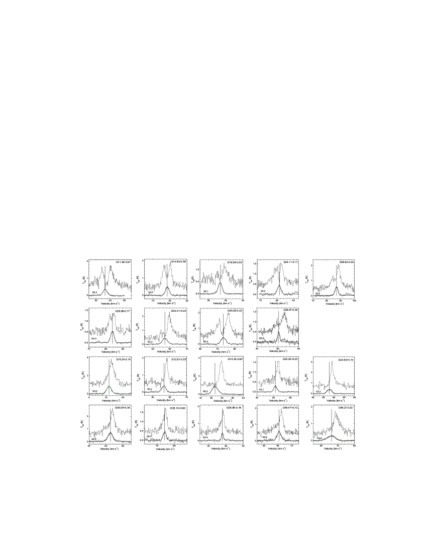
Figure 2: The same as Figure 1 but for 19 red profile candidates. The upper two rows show 9 sources with double-peaked spectra, and the lower two rows show 10 sources with skewed spectra.

The parameters T_MB(B)/T_MB(R), $\delta v$ with their uncertainties for 69 sources in our analysis sample derived from above two methods are given in Table 7. For double-peaked profile, we used the velocity at the brightest peak as the value of $v_{thick}$ to calculate $\delta v$. Following Mardones et al. (1997) we also adopt $\delta v$ of $\pm$0.25 (also corresponding to 5 times the typical rms error in $\delta v$ listed in column (2) of Table 7.) as the threshold to define the line asymmetries. As for brightness ratio method, we consider an asymmetry to be significant if the difference (or sum) between T_MB(B)/T_MB(R) and its uncertainty is still larger (or less) than 1 for blue (or red) double-peaked profile. Finally we identify 29 blue asymmetric profile candidates (including 20 double-peaked profiles and 9 skewed profiles) and 19 red asymmetric profile candidates (including 9 double-peaked profiles and 10 skewed profiles). The remaining 21 sources do not show significantly asymmetric profiles. Note that all 20 blue double-peaked profiles or all 9 red double-peaked profiles can also be defined as blue or red profiles based on the $\delta v$ method. That is, the blue or red profiles identified by the brightness ratio method is a subset of the blue or red profiles identified by the $\delta v$ method. The profile asymmetries for all the 69 sources are summarized in column (4) of Table 7. For seeing clearly the HCO⁺ asymmetry characteristics, we show the HCO⁺ and C¹⁸O spectra of 29 blue profile candidates and 19 red profile candidates in Figures 1 and 2, respectively. The spectra of the remaining 21 sources with no significantly asymmetric profiles, as well as the 3 sources with complex HCO⁺ or C¹⁸O spectra are shown in Figure 3. We also give the ¹²CO and ¹³CO spectra of all the 72 sources in an online figure.

In our observations, the optically thin C¹⁸O line shows an ideal Gaussian profile and is fitted by the Gaussian function to obtain the line center velocity and width. We also simply estimate the optical depth for C¹⁸O based on Myers et al. (1983) method:

$$\frac{(T_{MB})_{13}}{(T_{MB})_{18}}=\frac{1-exp(-5.5\tau_{18})}{1-exp(-\tau_{18})},$$ (1)

where (T_MB)₁₃ and (T_MB)₁₈ are the peak main beam temperature of ¹³CO and C¹⁸O; $\tau_{18}$ is the optical depth of C¹⁸O. This method was widely adopted in the analysis for dark clouds that usually show strong ¹²CO line self-absorption or blended profile due to background emission. Thus this method should well adapt to our cases as most sources in our observations also show apparent ¹²CO line self-absorption or blended profiles. However when $(T_{MB})_{13}/(T_{MB})_{18}>5$ appears in our calculations, the derived optical depth of C¹⁸O seems unreasonably small (this would lead to a larger value of excitation temperature). For these cases (marked by “b” in Table 6) we adopted the typical LTE method to estimate the optical depth using ¹²CO peak temperature (e.g. Sato et al. 1994). The derived optical depth of C¹⁸O is listed in column (5) of Table 7. It can be seen that for all sources the optical depth is less than 1 with a mean of 0.2. This suggests the C¹⁸O line is indeed optically thin in our sample, therefore it can reach the region near the centre of collapsing core and can be used to determine the system velocity.

Another question about using C¹⁸O to determine the line center velocity comes from whether HCO⁺ and C¹⁸O lines are tracing the same material. From Figures 1, 2 and 3, it can be clearly seen that C¹⁸O can accurately trace the line center velocity in all sources except for G49.27-0.34 as shown in Fig. 3. From its HCO⁺ spectrum, G49.27-0.34 seems to show a blue profile somewhat with a self-absorption dip at velocity of 71.5 km s^-1, while the line center velocity determined from C¹⁸O is 67.8 km s^-1. This source is considered to be the non-asymmetric profile based on the $\delta v$ method in our work. It suggests that C¹⁸O emission should trace the same material as HCO⁺ line and thus be good to determine the center velocity of HCO⁺ line. Moreover some mapping observations of HCO⁺ ($1-0$) and C¹⁸O (1-0) lines also provide the evidence that both lines can trace the same emission region (e.g. Qi et al. 2003; Wu et al. 2009). Sun & Gao (2008) also suggest that ¹³CO and C¹⁸O lines can be used to measure the line center velocity of HCO⁺ with the same PMO-13.7 m telescope.

Comparison with the high transition HCO⁺ (3–2) spectra acquired with the James Clerk Maxwell Telescope (JCMT) by Cyganowski et al. (2009), we surprisingly found that only 3 sources show the same line profile classification of blue/red or non-asymmetric profiles in a total of 17 common sources (comparing Table 7 in our work with Table 6 in Cyganowski et al. 2009). One possibility for such a difference between two studies is that the spectral resolution of HCO⁺ (3–2) of $\sim$0.6 km s^-1 is different from our HCO⁺ (1–0) spectra with $\sim$0.2 km s^-1. For checking this, we only consider 6 sources (G11.92-0.61, G19.36-0.03, G22.04+0.22, G28.28-0.36, G28.83-0.25 and G35.03+0.35) with clear HCO⁺ (3–2) self-absorption dips. But there are still 3 sources (G19.36-0.03, G28.28-0.36 and G35.03+0.35) show contrary profile classifications. It suggests that the spectral resolution difference is not the major factor for the profile classification difference in the two studies. Another possibility is a larger beam (80^′′) used in our HCO⁺ (1–0) observations relative to 19^′′ in the JCMT HCO⁺ (3–2) observations. However all the 9 overlapped sources between our survey and Purcell et al. (2006) survey show similar HCO⁺ (1–0) profile even though the two surveys have different beam sizes (see §3.1). And none of all the 5 sources overlapped among the three surveys (HCO⁺ (1–0) by our observation and Purcell et al. 2006, HCO⁺ (3–2) by Cyganowski et al. 2009) shows the same profile classifications based on HCO⁺ (1–0) and HCO⁺ (3–2) spectra. Thus combining these factors, it is most likely that the different transitions of HCO⁺ may trace different gas circumstances and need different excitation conditions to shape the corresponding blue or red profiles. This point has also been reported by Fuller et al. (2005) and Wu et al. (2007) that showed the different line asymmetries of HCO⁺ at transitions of (1–0) and (3–2) in some observed sources.

3.3 Blue Profile Excess Quantity

Most mechanisms that can produce asymmetric line profiles towards sources, e.g. rotation, outflow, should have approximately equal numbers of red and blue profiles, except that infall preferentially produces blue profiles. To quantify whether blue profile dominates in a sample, Mardones et al. (1997) defined a quantity E, the blue excess: $E=(N_{blue}-N_{red})/N_{total}$, where $N_{blue}$ and $N_{red}$ are the number of sources which show blue or red profiles, respectively, and $N_{total}$ is the total numbers of sample sources. Since then, the blue excess quantity has been widely adopted in line asymmetry analysis (e.g. Wu & Evans 2003, Fuller et al. 2005, Purcell et al. 2006, Wu et al. 2007). To compare with other surveys we also adopt the blue excess quantity analysis in our sample. In order to see the blue excess more clearly, we plot the T_MB(B)/T_MB(R) and $\delta v$ of HCO⁺ distributions in Figure 4. The blue excess using the $\delta v$ and brightness ratio methods is (29-19)/69=0.14 and (20-9)/69=0.16, respectively and with corresponding probability, $P$, of 0.09 and 0.02 that arises by chance. The probability, $P$ that the blue excess arises by chance is estimated with the binomial test (see Fuller et al. 2005 and references therein). We adopted the blue excess value derived from $\delta v$ method because this can identify a relatively large number of sources with line asymmetry. The statistical results are summarized in Table 8.

4 Discussion

4.1 Blue Profile Excess in Different Sample

The blue excess in our EGO sample is similar to that reported in Fuller et al. (2005). They also found the blue excess of 0.15 with the same HCO⁺ (1–0) line in a sample of 77 MYSOs with distances ranged from 1 to 10 kpc and associated with 850 $\mu$m emission. However, these values are distinctly smaller than the results reported in other surveys. For comparison, Wu & Evans (2003) found 12 blue profile candidates and measured a blue excess of 0.29 among a sample of 28 MYSOs with distances spanned a range of 1 – 12 kpc and associated with water masers; Wu et al. (2007) detected blue profiles in 17 cores and blue excess of 0.29 within a sample of 46 MYSOs associated with precursors of UC Hii and UC Hii regions and with distances ranged from 0.5 to 10 kpc. Whereas the blue excess of 0.14 found in our survey is slightly higher than that reported by two recent major HCO⁺ (1–0) studies of 6.7 GHz methanol maser sources by Purcell et al. (2006) and Szymczak et al. (2007). They found that approximately equal numbers of red and blue profiles, i.e. no infall signatures in their survey. For understanding the blue excess obtained in our survey and comparing with other surveys in detail, we divided our sources into some sub-samples as follows.

4.1.1 Distance Effect

Fuller et al. (2005) suggested that the lower blue excess value found in their work is most likely because the telescope beam may contain emission from material not intimately associated with MYSOs for those at larger distances. To limit this possibility, they carried out the analysis for sources with distances of less than 8 kpc, and found blue excess of HCO⁺ (1–0) line to be 0.28. We performed such an analysis to minimize the distance effect. We used new galactic rotation curve (Reid et al. 2009) to calculate the kinematic distances, assuming the galactic constants, R${}_{\odot}=$ 8.4 kpc and $\Theta_{\odot}=$ 254 km s^-1. The system velocity was determined from Gaussian fits to the C¹⁸O line. Most sources lie inside the solar circle and thus may have a near/far distance ambiguity, the near kinematic distances were adopted for these sources in our analysis, and listed in column (6) of Table 7. However the distances for four sources (G49.07-0.33, G49.27-0.32, G49.27-0.34 and G59.79+0.63) can not be derived from the galactic rotation curve, 5 kpc was assumed. The distances of most sources span a range of 2-6 kpc except for two sources (G12.02-0.21 and G49.42+0.33) with distances of larger than 12 kpc. For comparison, a distance of 4 kpc was adopted as a limit, which is compared to 8 kpc adopted in Fuller et al. (2005) with a telescope beam of $\sim 30\arcsec$. We formed a sub-sample of 31 objects with distances of less than 4 kpc and have looked at the blue excess for these objects alone. For this distance limited sub-sample, 12 blue profile candidates and 10 red profile candidates were found – thus an even smaller blue excess of only 0.06 with a probability of 0.58 appeared (see Table 8). It suggests that the far distance effect did not play an important role in understanding the relatively small blue excess in our sample. However, the adopted near kinematic distance may not be very reliable. If the red profile candidates have larger distances i.e. at far kinematic distances, a higher blue excess would be expected. Another possible explanation for relatively small blue excess even after considering the distance effect is the small EGO size with typical less than 30″ seen from their IRAC images, which makes the telescope beam still encompass the emission from material not intimately associated with MYSOs even at smaller distances.

4.1.2 “Likely” and ”Possible” Outflow Candidates

According to Cyganowski et al. (2008), the 69 sample sources used in our line asymmetry analysis include 41 “likely” MYSO outflow candidates and 28 “possible” MYSO outflow candidates. We performed the blue excess analysis for the sub-samples of “likely” and “possible” outflows, respectively. We found 14 blue profiles and 12 red profiles of 41 “likely” outflow candidates, and 15 blue profiles and 7 red profiles of 28 “possible” outflow candidates. Thus the blue excess seen in “likely” and “possible” outflow candidates is 0.05 and 0.29, respectively with corresponding probability of 0.42 and 0.07 (see Table 8). The blue excess in “likely” sub-sample is distinctly smaller than that in “possible” sub-sample. The appearance of very low blue excess in “likely” sub-sample is most likely because these sources are dominated by outflows. The distinct extended 4.5 $\mu$m emission around these sources identified from IRAC images suggests that they should be associated with strong and distinct outflows, thus were classified into the “likely” MYSO outflow candidates by Cyganowski et al. (2008). The significant outflows may be shaping more red profiles which results in weakening the blue excess. On the other hand the relatively high blue excess of 0.29 found in “possible” outflow sub-sample similar to the typical value found in other surveys (e.g. Wu & Evans 2003, Wu et al. 2007) suggests that the outflows may be weak and unobvious in “possible” sub-sample compared to “likely” sub-sample, consistent with the outcomes seen in IRAC images (Cyganowski et al. 2008).

We also found that 18 of 42 “likely” outflow candidates, and 12 of 30 “possible” outflow candidates show broad HCO⁺ line wing emissions, suggesting the possible existence of outflow among these sources (note that additional 1 “likely” and 2 “possible” outflow candidates that were not used in the line asymmetry analysis are included in this statistics). But the detection rates of outflow traced by HCO⁺ line wings are similar in both “likely” outflow sub-sample (18/42=43%) and “possible” outflow sub-sample (12/30=40%). Thus it seems that the HCO⁺ line wing emissions are not sensitive to the outflow classifications (i.e. “likely” and “possible”) seen from the IRAC images.

4.1.3 IRDCs and non-IRDCs

We also divided our sample into two sub-samples depending on their association with IRDCs. Usually IRDCs are believed to be potential sites of massive star formation and represent early stage of massive star formation. There are 12 blue profiles and 15 red profiles, and thus a negative blue excess of -0.08 with a chance probability of 0.65 existed among 37 IRDC sources, whereas 17 blue profiles and 4 red profiles, and a blue excess of 0.41 with a small chance probability of 0.004 were found among 32 non-IRDC sources. The statistical results are also given in Table 8.

The blue excess found in IRDC sub-sample is much smaller than that in non-IRDC sub-sample. One explanation for different blue excess between them is that the infall signatures may be different at different evolutionary stages of massive star formation. Actually the relation between blue profile excess and evolutionary phase has been studied in low- and high-mass star forming regions (e.g. Mardones et al. 1997, Wu et al. 2007). In low-mass cores the blue excess was found to be 0.30, 0.31, and 0.31 for –I, 0, and I core samples, respectively (Evans 2003 and references therein). There seems to be no significant difference among different evolutionary phases of low-mass star formation. In massive star forming cores, UC Hii regions show a higher blue excess (0.58) than UC Hii precursors (0.17), indicating that material is still accreted after the onset of the UC Hii phase and there has a higher blue excess at the stage with hot cores (Wu et al. 2007). This may point to fundamental difference between low- and high-mass star forming conditions. In our observations, the very low or negative blue excess detected in the early evolutionary stage sources associated with IRDCs can be explained as follows: (1) the molecular gas in IRDCs surrounding EGOs (i.e. earlier stage sources) may not be adequately thermalized to show the blue excess; (2) The amount of dense cool gas is larger toward younger objects. Outflows of dense molecular gas may be more active around IRDC sources, shaping more red profiles. One evidence for this is that most (26/41=63%) “likely” outflow candidates are associated with IRDCs. There is also a slightly higher detection rate of the outflow traced by HCO⁺ line wing of 18/38=47% in IRDC sub-sample than that of 12/34=35% in non-IRDC sub-sample (here in both sub-samples, we include additional 1 IRDC and 2 non-IRDC sources that were not used in the line asymmetry analysis). These suggest that the outflows are indeed more active around IRDC sources at very early evolutionary stage of massive star formation, and thus shaping more red profiles and resulting in lower blue excess. Comparison with IRDCs, the higher blue excess found in non-IRDCs may be due to that these sources are at a relatively late stage of massive star formation. However, we have no justification to believe that sources not associated with IRDCs must be located at the late evolutionary stage. The visibility of an IRDC is dependent on the strength of the mid-infrared background emission particularly at 8 $\mu$m (Cyganowski et al. 2008). If there is no or weak 8 $\mu$m emission in a particular region, non-IRDC may be visible, even if dense molecular gas and very young MYSOs are present.

Some other factors could not be neglected to understand the different blue excess between IRDC and non-IRDC sub-samples. For example, molecular material in the IRDC but not directly physically associated with the EGO may contribute significantly to the emission within the large beam. Dynamical interactions between outflows and surrounding molecular material in IRDC sub-sample may be very different from those in non-IRDC sub-sample. Both above possibilities would affect the line profiles and result in different observed blue excess. Moreover, the lower blue excess in IRDC sub-sample seems to be also explained if EGO associated with IRDC is in the cluster environment and wherein the competitive accretion is occurred. As Bonnell & Bate (2006) suggested, the larger tangential velocities and the velocity dispersion presented in the cluster environments would reduce the infall signatures under the competitive accretion. Obviously, our current single-pointing observations with a large beam can not give answers to any possibilities described as above. Higher-angular resolution data are needed to clarify these possibilities.

4.1.4 6.7 GHz methanol masers and UC Hii Regions

In addition, our sample is also associated with other astrophysical objects, e.g. UC Hii regions and 6.7 GHz class II methanol masers. We carried out the blue excess analysis for these sub-samples with the statistical results also listed in Table 8. We found that the blue excess in UC Hii regions ($\sim 0.19$) is slightly higher than that in 6.7 GHz methanol maser sources ($\sim 0.07$). The different blue excess in these two sub-samples seems also to be due to that the blue excess may evolve with the different massive star formation stage as described in above section. The 6.7 GHz class II methanol masers are only associated with MSFRs and also trace an early evolutionary stage, as evidenced by their association with IRDCs (Ellingsen 2006) and millimeter and submillimeter dust continuum emission (Pestalozzi et al. 2002; Walsh et al. 2003). Thus the blue excess could be lower in 6.7 GHz methanol maser sub-sample due to not adequately thermalized gas in the centre of the core at the earlier stage. Two recent HCO⁺ surveys of 6.7 GHz methanol maser sources by Purcell et al. (2006) and Szymczak et al. (2007) that also found no or very low blue excess in their samples are consistent with our statistical result.

As stated in previous section, Wu et al. (2007) found a higher blue excess (0.58) in UC Hii regions. However the blue excess in UC Hii regions detected in our survey is quite lower. One possibility is that the sources associated with UC Hii regions may be at a range of evolutionary stages. For clarifying this, we exclude the possible younger sources associated with both UC Hii region and methanol maser in our analysis. Interestingly, we found 5 blue profiles and only 1 red profile among a total of 6 sources that are only associated with UC Hii region and are believed to be at late evolutionary stage, thus the blue excess is as high as 0.67. Such a high blue excess is in agreement with that reported by Wu et al. (2007).

Combining above results from our survey and other surveys, it seems that the blue excess evolving with different stage may be a genuine characteristic of massive star formation. However the small samples of UC Hii region (16) and methanol maser (25) and the larger chance probabilities of blue excess (0.3-0.4) in our surveys (see Table 8) should be taken into account before drawing any definite conclusions. It should be noted that not all of the observed northern EGOs have been searched for UC Hii regions or 6.7 GHz methanol masers (not all fall within the coverage of large blind surveys for these tracers), thus there may be a bias in the known associations of EGOs with these tracers.

4.2 Physical Properties of the EGOs

Cyganowski et al. (2008) argued that GLIMPSE-identified EGOs are only associated with high-mass star formation based on their association with other high-mass star formation tracers such as IRDCs and class II methanol masers, and that the surface brightness of low-mass outflows will be too faint to be detected at the sensitivity of the GLIMPSE survey, even though the extended 4.5 $\mu$m could also be seen towards nearby low-mass outflows as well by deep observations (e.g. Noriega-Crespo et al. 2004). Chen et al. (2009) analyzed the EGOs searched for class I methanol masers (61 in total) and found that class I methanol masers were detected towards about two-thirds of EGOs, also suggesting that EGOs are associated with outflows from MYSOs. Moreover comparison with recent published 1.1 mm continuum BOLOCAM GPS catalog (Rosolowsky et al. 2009), we found that most (65/77=84%; see Table 1) EGOs in our observed sample are associated with mm continuum source within 30^′′ (corresponding to half the PMO beam size). The detected mm continuum emission, especially in IRDCs, suggests that EGOs pinpoint the sites of massive star formation at early evolutionary stage (Rathborne & Jackson 2006). However, the physical properties of the EGOs such as gas density and mass etc. are still unclear.

To understand their physical properties, we calculated the parameters with C¹⁸O line following the typical LTE method (e.g. Sato et al. 1994). The physical parameters derived from C¹⁸O line are also given in Table 7. The typical size of EGO of a few to 30^′′ seen from IRAC images is smaller than the beam size of the telescope. Thus it is very likely that the C¹⁸O emitting region is too small to fully fill in the whole telescope beam. We determined the beam filling factor, $f$, for each source with the same method adopted in Klaassen & Wilson (2007) that assumed a consistent ambient temperature for all the observed sources (Eq. 2 in their work). In our observed EGOs, one source G34.26+0.15 has a similar scale ($\sim$ 60^′′ seen from its IRAC image) to the telescope beam size, we assumed the beam filling factor is 1 for this source. Under this assumption and Eq. (2) of Klaassen & Wilson (2007), an ambient temperature of 30 K was derived for this source. We adopted this ambient temperature to all the other observed EGOs. The derived beam filling factor for each source is listed in the column (7) of Table 7. And then the angular size of the C¹⁸O emitting region was estimated from the beam size and beam filling factor. Linear size (column (8) in Table 7) was calculated from the angular size and kinematic distance (column (6) in Table 7). The mean size of the C¹⁸O emitting region is 0.8 pc (typically 0.5-1 pc). The derived mean column density of C¹⁸O (column (9) in Table 7) is $3\times 10^{16}$ cm^-2. The column density of H₂ is derived with a moderate C¹⁸O abundance of $1.7\times 10^{-7}$ (Frerking et al. 1982). The mean column density of H₂ (column (10) in Table 7) is $2\times 10^{23}$ cm^-2, while the mean volume density (column (11) in Table 7) is $1.5\times 10^{5}$ cm^-3. The LTE masses based on C¹⁸O (column (12) in Table 7) range from a few 100 to several 1000 M_⊙ with a mean mass of $2\times 10^{3}$ M_⊙ (this mass range is very similar to that for the sample of 6.7 GHz methanol maser sources and UC Hii regions reported by Purcell et al. (2009)). All above physical parameters are consistent with the characteristics of the massive clumps wherein massive star forming cores associated with EGOs possibly embedded (e.g. Beuther et al. 2007). Here we follow Beuther et al. (2007) to define the terms clump and core: clump for condensations associated with cluster formation, and core for molecular condensations that form single or gravitationally bound multiple massive protostars. Moreover, the physical properties of sources associated with IRDCs in our sample are also consistent with those reported in previous IRDC studies, e.g. Carey et al. (1998, 2000) with the column density as high as $10^{23}$ cm^-2 and gas density $\sim 10^{5}-10^{6}$ cm^-3. These physical properties are consistent with the speculation of Cyganowski et al. (2008) that EGOs are MYSOs.

However, the physical parameters derived here may not be very reliable as the assumption of the uniform ambient temperature for all sources and the derived sizes under this assumption may not reflect the actual temperatures and molecular cloud sizes for the observed sources. Especially when other sources in addition to EGOs are present within the telescope beam, the emission from other sources will contribute to the derived physical parameters e.g. sizes and masses of EGOs. Thus the derived physical parameters should be treated as upper limits.

4.3 Accretion Properties of Infall Candidates

We can measure an infall velocity (V_in) using the two layer radiative transfer model of Myers et al. (1996; Eq. (9) of their work) for each of the 20 sources with blue, double-peaked HCO⁺ profiles identified in §3.2. Then we can use Eq. (3) of Klaassen & Wilson (2007) to calculate the mass infall rate Ṁ_in for each of them. The infall velocity and mass infall rate are summarized in Table 9. In this calculation, the C¹⁸O line width (column (14) of Table 6) was adopted as a measure of the velocity dispersion in the circumstellar material, and the ambient density n(H₂) is assumed to be the gas density of cloud determined from CO line listed in column (11) of Table 7. From our rms uncertainties in temperatures and one-half the spectral resolution of our observations, we determined the uncertainties of the infall velocity and infall rate for each source. From this analysis, we determined the infall velocities ranging from 0.5 to 8 km s^-1 with a mean value of 2 km s^-1, and the mass infall rates ranging from $4\times 10^{-2}$ to $1\times 10^{-4}$ M_⊙ yr^-1. The infall velocities obtained in our observations are somewhat higher than those presented in Fuller et al. (2005) and Klaassen & Wilson (2007, 2008) with a typical value of $<$1.5 km s^-1. This could be due to our larger telescope beam that might contain more outer material of the cloud with large LOS velocity to produce somehow larger observable infall velocity. Thus, the calculated infall velocities may be treated as the upper limit in our observations. The infall rates derived here are higher than those observed for low-mass star forming regions, but are consistent with that determined in other surveys of MYSOs (Fuller et al. 2005; Klassen & Wilson 2007, 2008) and the theoretical accretion rates for massive star forming cores (McKee & Tan 2003; Bonnell & Bate 2006).

Usually the mass outflow rates are also orders of magnitude higher in high-mass star forming regions than that in low-mass star forming regions (e.g. Beuther et al. 2002). Fuller et al. (2005) suggested that the infall rates are consistent with the outflow rates in their survey, but Klaassen & Wilson (2007) found that the ratio of the mass outflow rate to infall rate to be Ṁ_in/Ṁ_out$\approx$1/16 for the UC Hii source Cep A. In our survey, the mass outflow rates for only two of infall double-peaked profile sources (G16.59-0.05, G35.20-0.74) are presented by Wu et al. (2004) catalog of high-velocity outflows. We find the ratio of Ṁ_in/Ṁ_out to be $2-3$ for the two sources, much higher than that reported by Klaassen & Wilson (2007). Behrend & Maeder (2001) have suggested that the Ṁ_in/Ṁ_out ratio is probably nonconstant during the evolution of accreting stars, and could be a decreasing function of the stellar mass. Combining these factors, we suggest that the EGOs in our survey should be at very earlier evolutionary stage of massive star formation and the centre protostellar mass could rapidly increase with a higher ratio value of Ṁ_in/Ṁ_out compared to the case of UC Hii Cep A at late evolutionary stage reported by Klaassen & Wilson (2007). This property is also consistent with the inference of Cyganowski et al. (2008) that EGOs trace the active rapid accretion earlier stage of massive protostellar evolution. However the ratio value of Ṁ_in/Ṁ_out obtained in our observations may be overestimated due to the large beam.

4.4 The Limitations for Single-Pointing-Only Surveys

In this section, we give some discussions or summarizations for the limitations to our single-pointing-only survey. We can only detect the possible infall and outflow dynamics from the spectral profile (blue profile and line wing) with single-pointing observations. But the actual emission regions of infall and outflow could not be determined, thus we could not give more information to understand the dynamics properties of EGOs. We could not measure the actual observed mm line emitting regions, although these regions could be simply estimated by the assumption of the uniform ambient temperature for all sources. But these estimated regions might not trace the true sizes of molecular clouds around EGOs as discussed in §4.2. Thus the derived physical parameters (i.e. gas density and mass) of EGO and infall velocity and rate of infall candidates might not reflect the true cases for EGOs. Especially, the large beam in our observations would bring large limitations for the studies. We could not exclude absolutely that the observed emission might be dominated by other sources in addition to EGOs within the large beam. The HCO⁺ line profiles could be affected if there are multiple sources all of which contribute to the emission within the beam. We also can not determine whether there are multi-core or only one core to form massive star within EGO regions. We can only say that the derived physical properties actually trace a relatively large regions (or clumps) therein EGOs embedded. Moreover our single-pointing-only survey with a large beam still can not answer where and how the infall dynamics has happened, in an isolated core (monolithic collapse) or in a protocluster (competitive accretion). Though we have determined a significant blue excess suggesting infall signature in full observed EGO sample, some very low or negative blue excess have also been detected in some particular populations, e.g. IRDC, and class II methanol maser sub-samples. We could not obviate the possibility that the competitive accretion might have been occurred in such populations possibly associated with cluster environments, because the competitive accretion theory also suggests that the infall may be not statistically significant due to larger velocity dispersion in complex cluster environments (Bonnell & Bate 2006). Future high-resolution observations are very important for detecting the accretion scale to investigate which is the dominant accretion dynamics in EGOs.

5 Conclusion

Using the PMO-13.7 m radio telescope, we performed the first systematic molecular line (including HCO⁺ and CO lines at 3 mm band) survey toward a new MYSO sample of 88 EGOs in the northern hemisphere identified from Spitzer GLIMPSE survey to search for infall evidence and understand the physical properties in these sources. We detected HCO⁺ emission in 72 sources. By analyzing the line profiles of the optically thick line HCO⁺ and the optically thin line C¹⁸O for 69 of 72 sources, we identified 29 blue profile candidates with 20 double-peaked profiles and 9 skewed profiles and, 19 red profile candidates with 9 double-peaked profiles and 10 skewed profiles. Thus a blue profile excess of about 0.14 was measured, suggesting that the infall is statistically significant in our EGO sample. This value is somewhat different from other surveys towards MYSOs selected from different criteria, e.g. 6.7 GHz class II methanol masers or UC Hii regions. The blue excess analysis in different sub-samples was then performed to understand the different blue excess values among our survey and other surveys. We found that the sources not associated with IRDCs show a higher blue excess (0.41) than those associated with IRDCs (-0.08), the “possible” outflow candidates also show a higher blue excess (0.29) than “likely” outflow candidates (0.05), and the blue excess (0.19) found in UC Hii regions is higher than that in 6.7 GHz class II methanol masers (0.07). These statistical results suggest that a relatively small blue excess determined in our observations is mainly because that most observed EGOs are dominated by outflows and are at an early evolutionary stage associated with IRDCs and 6.7 GHz methanol masers. By combining the statistical results from our survey and with those from other surveys, we point out that the infall signatures gradually evolving with the different stage may be a genuine property of massive star formation: the blue excess is not statistically significant in the earlier evolutionary stage associated with IRDCs or 6.7 GHz class II methanol masers, and the blue excess will gradually become to be statistically significant with massive star formation evolution, especially when arriving at the later evolutionary stage associated with UC Hii region.

Furthermore, the physical properties of EGOs are derived using CO lines. Typical size of the cloud surrounding EGO is 0.8 pc, typical column density is $2\times 10^{23}$ cm^-2, typical volume density is about $2\times 10^{5}$ cm^-3, and typical mass is about $2\times 10^{3}$ M_⊙, all of which are similar to those of massive clump wherein massive star forming cores associated with EGO possibly embedded. These physical properties support the speculation of Cyganowski et al. (2008) that EGOs are associated with MYSOs. The estimated infall velocities (typically 2 km s^-1) and mass infall rates ($4\times 10^{-2}$ to $1\times 10^{-4}$ M_⊙ yr^-1) for 20 sources with blue double-peaked profiles are also consistent with that determined in other surveys for MSFRs and the theoretical values. The higher ratio values of Ṁ_in/Ṁ_out$\sim$($2-3$) measured in two sources (G16.59-0.05, G35.20-0.74) may also suggest that the EGOs in our survey should be at very earlier evolutionary stage of massive star formation and the centre protostellar mass could rapidly increase. However the physical and infall parameters may be overestimated due to the single-pointing observations with a large beam.

Though there are some limitations due to our single-pointing-only survey with a large beam for studying the EGOs at present, this survey still offers useful information to our investigating the properties of EGOs from the statistical view. It provides a working sample to study the EGOs with high-resolution observations in future.

Table 1: Sample parameters

	Positiona
Source	R.A. (2000)	Dec. (2000)	IRDCb	CH3OHc	UC Hiic	1.1 mmc	Remarkd
	(h m s)	(° ′ ″)
G10.29-0.13	18 08 49.3	-20 05 57	Y	Y	–	Y	2
G10.34-0.14	18 09 00.0	-20 03 35	Y	Y	–	Y	2
G11.11-0.11	18 10 28.3	-19 22 31	Y	–	–	Y	3
G11.92-0.61	18 13 58.1	-18 54 17	Y	Y	–	–	1
G12.02-0.21	18 12 40.4	-18 37 11	Y	–	–	Y	1
G12.20-0.03	18 12 23.6	-18 22 54	N	Y	–	Y	4
G12.42+0.50	18 10 51.1	-17 55 50	N	–	Y	Y	4
G12.68-0.18	18 13 54.7	-18 01 47	N	Y	–	Y	4
G12.91-0.03	18 13 48.2	-17 45 39	Y	–	–	Y	1
G12.91-0.26	18 14 39.5	-17 52 00	N	Y	Y	Y	5
G14.33-0.64	18 18 54.4	-16 47 46	Y	N	Y	–	1
G14.63-0.58	18 19 15.4	-16 30 07	Y	–	–	Y	1
G16.58-0.08	18 21 15.0	-14 33 02	Y	N	–	Y	3
G16.59-0.05	18 21 09.1	-14 31 48	Y	Y	Y	Y	2
G16.61-0.24	18 21 52.7	-14 35 51	Y	–	–	Y	1
G17.96+0.08	18 23 21.0	-13 15 11	N	–	–	Y	4
G18.67+0.03	18 24 53.7	-12 39 20	N	Y	–	Y	1
G18.89-0.47	18 27 07.9	-12 41 36	Y	Y	–	Y	1
G19.01-0.03	18 25 44.8	-12 22 46	Y	Y	–	Y	1
G19.36-0.03	18 26 25.8	-12 03 57	Y	Y	Y	Y	2
G19.61-0.12	18 27 13.6	-11 53 20	N	Y	–	N	2
G19.88-0.53	18 29 14.7	-11 50 23	Y	–	–	Y	1
G20.24+0.07	18 27 44.6	-11 14 54	N	Y	–	Y	4
G21.24+0.19	18 29 10.2	-10 18 11	Y	–	–	Y	4
G22.04+0.22	18 30 34.7	-09 34 47	Y	Y	–	Y	1
G23.01-0.41	18 34 40.2	-09 00 38	N	Y	–	Y	1
G23.82+0.38	18 33 19.5	-07 55 37	N	–	–	Y	4
G23.96-0.11	18 35 22.3	-08 01 28	N	Y	–	Y	1
G24.00-0.10	18 35 23.5	-07 59 32	Y	Y	Y	Y	1
G24.11-0.17	18 35 52.6	-07 55 17	Y	–	–	Y	4
G24.17-0.02	18 35 25.0	-07 48 15	Y	Y	–	N	1
G24.33+0.14	18 35 08.1	-07 35 04	Y	Y	–	Y	4
G24.63+0.15	18 35 40.1	-07 18 35	Y	–	–	Y	3
G24.94+0.07	18 36 31.5	-07 04 16	N	Y	–	Y	1
G25.27-0.43	18 38 57.0	-07 00 48	Y	Y	–	Y	1
G25.38-0.15	18 38 08.1	-06 46 53	Y	–	Y	Y	2
G27.97-0.47	18 44 03.6	-04 38 02	Y	–	–	Y	1
G28.28-0.36	18 44 13.2	-04 18 04	N	Y	Y	Y	2
G28.83-0.25	18 44 51.3	-03 45 48	Y	Y	Y	Y	1
G28.85-0.23	18 44 47.5	-03 44 15	N	Y	–	N	4
G29.84-0.47	18 47 28.8	-02 58 03	Y	–	–	Y	3
G29.89-0.77	18 48 37.7	-03 03 44	Y	–	–	–	4
G29.91-0.81	18 48 47.6	-03 03 31	N	–	–	Y	4
G29.96-0.79	18 48 50.0	-03 00 21	Y	–	–	Y	3
G34.26+0.15	18 53 16.4	+01 15 07	N	–	Y	N	5
G34.28+0.18	18 53 15.0	+01 17 11	Y	–	–	Y	3
G34.39+0.22	18 53 19.0	+01 24 08	Y	–	–	N	2
G34.41+0.24	18 53 17.9	+01 25 25	Y	–	Y	Y	1
G35.03+0.35	18 54 00.5	+02 01 18	N	Y	Y	Y	1
G35.04-0.47	18 56 58.1	+01 39 37	Y	–	–	Y	1
G35.13-0.74	18 58 06.4	+01 37 01	N	–	–	–	1
G35.15+0.80	18 52 36.6	+02 20 26	N	–	–	–	1
G35.20-0.74	18 58 12.9	+01 40 33	N	–	–	–	1
G35.68-0.18	18 57 05.0	+02 22 00	Y	–	–	Y	1
G35.79-0.17	18 57 16.7	+02 27 56	Y	Y	–	Y	1
G35.83-0.20	18 57 26.9	+02 29 00	Y	–	–	Y	4
G36.01-0.20	18 57 45.9	+02 39 05	Y	–	–	Y	1
G37.48-0.10	19 00 07.0	+03 59 53	N	Y	–	Y	1
G37.55+0.20	18 59 07.5	+04 12 31	N	–	–	N	5
G39.10+0.49	19 00 58.1	+05 42 44	N	Y	–	Y	1
G39.39-0.14	19 03 45.3	+05 40 43	N	–	Y	Y	4
G40.28-0.22	19 05 41.3	+06 26 13	Y	–	–	Y	3
G40.28-0.27	19 05 51.5	+06 24 39	Y	–	–	Y	1
G40.60-0.72	19 08 03.3	+06 29 15	N	–	–	–	4
G43.04-0.45	19 11 38.9	+08 46 39	N	–	Y	Y	4
G44.01-0.03	19 11 57.2	+09 50 05	N	–	–	N	1
G45.47+0.05	19 14 25.6	+11 09 28	Y	Y	Y	Y	1
G45.47+0.13	19 14 07.3	+11 12 16	N	Y	Y	Y	4
G45.50+0.12	19 14 13.0	+11 13 30	N	Y	–	N	4
G45.80-0.36	19 16 31.1	+11 16 11	N	–	–	Y	3
G48.66-0.30	19 21 48.0	+13 49 21	Y	–	–	Y	2
G49.07-0.33	19 22 41.9	+14 10 12	Y	–	–	Y	3
G49.27-0.32	19 23 02.2	+14 20 52	N	N	–	N	3
G49.27-0.34	19 23 06.7	+14 20 13	Y	N	–	Y	1
G49.42+0.33	19 20 59.1	+14 46 53	N	Y	–	Y	2
G49.91+0.37	19 21 47.5	+15 14 26	N	–	–	Y	4
G50.36-0.42	19 25 32.8	+15 15 38	Y	–	–	N	3
G53.92-0.07	19 31 23.0	+18 33 00	N	–	–	Y	3
G54.11-0.04	19 31 40.0	+18 43 53	N	–	–	Y	4
G54.11-0.08	19 31 48.8	+18 42 57	N	–	–	Y	3
G54.45+1.01	19 28 26.4	+19 32 15	N	–	–	–	3
G56.13+0.22	19 34 51.5	+20 37 28	N	–	–	Y	1
G57.61+0.02	19 38 40.8	+21 49 35	N	–	–	Y	4
G58.09-0.34	19 41 03.9	+22 03 39	Y	–	–	N	1
G58.78+0.64	19 38 49.6	+23 08 40	N	–	–	–	4
G58.79+0.63	19 38 55.3	+23 09 04	N	–	–	–	3
G59.79+0.63	19 41 03.1	+24 01 15	Y	–	–	–	1
G62.70-0.51	19 51 51.1	+25 57 40	N	–	–	N	3

Table 2: List of observed lines

Line	Date	$\nu$	$\theta_{mb}$	$\eta_{mb}$	$\Delta v$
	(UT)	(GHz)	(arcsec)		(km s-1)
(1)	(2)	(3)	(4)	(5)	(6)
HCO+ (1-0)	2009 Jan 9-23	89.188518	80.6	0.50	0.205
12CO (1-0)	2009 Feb 12-17	115.271202	62.4	0.61	0.369
13CO (1-0)	2009 Feb 12-17	110.201353	65.3	0.60	0.114
C18O (1-0)	2009 Feb 12-17	109.782173	65.5	0.60	0.115

Note. — Col. (1): observed line. Col. (2): observational date. Col. (3): rest frequency. Col. (4): beam size. Col. (5): main beam efficiency. Col. (6): spectral resolution.

Table 3: Observed HCO⁺ (1–0) line properties of all 88 sample sources.

	Gaussian fits					Peak positions a
Source	$\int$T${}_{MB}dV$	VLSR	$\Delta V$	TMB		TMB	VLSR	$\sigma_{rms}$
	(K km s-1)	(km s-1)	(km s-1)	(K)		(K)	(km s-1)	(K)
(1)	(2)	(3)	(4)	(5)		(6)	(7)	(8)
G10.29-0.13b	8.43(0.21)	13.39(0.07)	5.66(0.17)	1.40		…	…	0.12
G10.34-0.14	9.20(0.50)	13.22(0.05)	3.87(0.16)	2.24		2.31	13.31	0.16
G11.11-0.11	5.18(0.52)	29.37(0.27)	5.96(0.48)	0.81		0.74	27.86	0.14
	…	…	…	…		0.31	33.58	…
G11.92-0.61	10.98(0.76)	37.66(0.10)	6.52(0.29)	1.58		1.08	34.25	0.16
	…	…	…	…		1.20	40.00	…
G12.02-0.21b	4.34(0.18)	-3.65(0.08)	3.99(0.20)	1.02		…	…	0.12
G12.20-0.03b	5.33(0.17)	51.09(0.06)	3.96(0.16)	1.26		…	…	0.12
G12.42+0.50	17.86(1.11)	17.58(0.03)	3.49(0.11)	4.77		4.23	16.76	0.16
G12.68-0.18c	0.56(0.11)	49.83(0.18)	1.82(0.42)	0.27		…	…	0.14
	3.38(0.16)	58.46(0.07)	3.29(0.16)	0.92		…	…	…
G12.91-0.03	2.84(0.14)	58.26(0.04)	2.04(0.13)	1.31		1.39	58.49	0.12
G12.91-0.26	15.47(1.28)	38.76(0.05)	5.19(0.68)	2.80		1.67	35.38	0.12
	…	…	…	…		0.87	42.91	…
G14.33-0.64	5.69(0.17)	24.64(0.03)	2.15(0.08)	2.49		2.70	24.70	0.16
G14.63-0.58	10.82(0.55)	18.33(0.04)	4.12(0.18)	2.45		1.18	16.46	0.12
	…	…	…	…		1.37	20.07	…
G16.58-0.08	2.70(0.70)	40.29(0.16)	2.90(0.37)	0.88		0.63	39.32	0.14
G16.59-0.05	14.10(0.68)	59.51(0.05)	3.09(0.10)	4.26		2.82	58.51	0.16
	…	…	…	…		1.82	60.06	…
G16.61-0.24d	—	—	—	—		—	—	0.18
G17.96+0.08	4.16(0.26)	22.46(0.05)	2.45(0.14)	1.60		1.19	21.67	0.12
	…	…	…	…		0.95	23.61	…
G18.67+0.03b	4.43(0.92)	79.69(0.15)	5.02(0.50)	0.83		…	…	0.10
G18.89-0.47b	15.28(1.69)	66.39(0.10)	5.03(0.52)	2.86		…	…	0.16
G19.01-0.03b	2.79(0.60)	60.61(0.08)	2.16(0.19)	1.22		…	…	0.16
G19.36-0.03	4.55(0.36)	28.09(0.19)	6.37(0.44)	0.67		0.40	25.39	0.12
	…	…	…	…		0.65	29.33	…
G19.61-0.12b	2.91(0.78)	57.37(0.13)	3.74(0.46)	0.73		…	…	0.10
G19.88-0.53b	14.20(0.85)	43.72(0.03)	3.59(0.12)	3.72		…	…	0.16
G20.24+0.07	1.82(0.18)	70.34(0.12)	2.76(0.43)	0.61		0.76	69.90	0.12
G21.24+0.19	6.80(1.43)	25.42(0.05)	2.58(0.20)	2.47		1.79	24.40	0.14
	…	…	…	…		0.93	26.81	…
G22.04+0.22	2.66(0.19)	52.67(0.08)	2.68(0.29)	0.93		1.09	52.89	0.14
G23.01-0.41	16.46(0.72)	76.12(0.12)	6.84(0.34)	2.25		1.70	73.66	0.14
	…	…	…	…		1.42	79.01	…
G23.82+0.38b	2.81(0.13)	75.89(0.08)	3.45(0.20)	0.76		…	…	0.10
G23.96-0.11d	—	—	—	—		—	—	0.20
G24.00-0.10	2.95(0.60)	71.73(0.14)	4.39(0.50)	0.63		0.61	70.49	0.12
G24.11-0.17	5.55(0.72)	81.05(0.10)	4.91(0.35)	1.05		0.71	79.47	0.12
	…	…	…	…		0.96	82.94	…
G24.17-0.02d	—	—	—	—		—	—	0.16
G24.33+0.14d	—	—	—	—		—	—	0.18
G24.63+0.15	8.82(0.71)	53.13(0.05)	3.23(0.15)	2.56		2.34	54.21	0.18
G24.94+0.07b	4.08(0.16)	41.42(0.09)	4.40(0.20)	0.87		…	…	0.12
G25.27-0.43b	1.77(0.11)	59.99(0.08)	2.50(0.20)	0.66		…	…	0.10
G25.38-0.15	9.23(0.49)	95.95(0.07)	5.35(0.20)	1.63		1.05	93.55	0.12
	…	…	…	…		0.64	99.06	…
G27.97-0.47d	—	—	—	—		—	—	0.20
G28.28-0.36	5.78(0.26)	48.67(0.09)	5.30(0.24)	1.02		0.88	47.06	0.12
	…	…	…	…		0.64	51.20	…
G28.83-0.25	8.79(0.77)	87.14(0.06)	4.89(0.22)	1.68		0.82	84.49	0.12
	…	…	…	…		1.50	88.63	…
G28.85-0.23c	2.83(0.18)	87.54(0.13)	4.37(0.30)	2.83		…	…	0.14
	1.45(0.15)	96.14(0.17)	3.34(0.39)	1.45		…	…	…
G29.84-0.47d	—	—	—	—		—	—	0.18
G29.89-0.77	4.53(0.16)	83.78(0.05)	3.19(0.12)	1.34		0.69	82.56	0.12
	…	…	…	…		0.83	84.93	…
G29.91-0.81	1.40(0.20)	83.67(0.20)	2.19(0.46)	0.60		0.74	83.06	0.12
	…	…	…	…		0.56	84.72	…
G29.96-0.79	3.62(0.64)	85.20(0.06)	2.17(0.18)	1.57		1.86	84.46	0.10
G34.26+0.15	33.00(2.31)	59.17(0.08)	6.80(0.18)	4.56		2.63	56.43	0.14
	…	…	…	…		0.64	65.13	…
G34.28+0.18	8.61(0.22)	58.62(0.06)	5.74(0.15)	1.41		0.93	56.12	0.10
	…	…	…	…		0.24	63.16	…
G34.39+0.22	5.04(0.38)	57.36(0.24)	4.46(0.70)	1.06		0.77	55.43	0.10
	…	…	…	…		0.54	61.35	…
G34.41+0.24	10.57(1.95)	58.17(0.07)	4.18(0.28)	2.38		0.44	54.43	0.12
	…	…	…	…		1.48	60.03	…
G35.03+0.35	8.70(0.70)	52.91(0.07)	4.59(0.22)	1.93		1.84	54.12	0.16
G35.04-0.47b	3.24(0.12)	51.44(0.05)	2.67(0.13)	1.14		…	…	0.10
G35.13-0.74b	44.98(0.19)	33.29(0.01)	5.53(0.03)	7.65		…	…	0.12
G35.15+0.80	3.74(0.14)	74.55(0.04)	2.69(0.12)	1.30		1.11	75.08	0.12
G35.20-0.74	25.97(0.60)	33.90(0.07)	8.28(0.20)	2.95		2.61	32.03	0.16
	…	…	…	…		1.56	37.59	…
G35.68-0.18	2.72(0.21)	26.63(0.86)	2.14(0.13)	1.20		1.14	28.80	0.12
G35.79-0.17d	—	—	—	—		—	—	0.18
G35.83-0.20b	1.95(0.22)	28.06(0.12)	3.04(0.60)	0.60		…	…	0.12
G36.01-0.20	2.37(0.26)	87.17(0.10)	2.46(0.23)	0.91		0.84	86.45	0.10
	…	…	…	…		0.46	88.46	…
G37.48-0.10b	3.36(0.15)	57.96(0.07)	3.03(0.15)	1.04		…	…	0.12
G37.55+0.20d	—	—	—	—		—	—	0.22
G39.10+0.49	3.75(0.33)	23.54(0.18)	5.47(0.46)	0.64		0.52	21.93	0.12
	…	…	…	…		0.35	25.79	…
G39.39-0.14	4.21(0.19)	65.97(0.08)	4.04(0.20)	0.98		1.05	65.71	0.12
G40.28-0.22	9.65(1.16)	74.22(0.08)	5.61(0.30)	1.62		0.82	70.58	0.14
	…	…	…	…		1.32	76.41	…
G40.28-0.27	1.97(0.19)	71.66(0.09)	2.33(0.24)	0.90		0.88	71.20	0.10
	…	…	…	…		0.66	72.81	…
G40.60-0.72b	4.86(0.18)	65.57(0.08)	4.58(0.21)	1.00		…	…	0.10
G43.04-0.45	3.46(0.16)	57.34(0.08)	4.08(0.20)	0.88		0.82	56.90	0.10
	…	…	…	…		0.46	59.58	…
G44.01-0.03b	2.83(0.13)	64.55(0.07)	3.14(0.17)	0.85		…	…	0.10
G45.47+0.05b	10.42(0.29)	60.28(0.15)	10.92(0.33)	0.90		…	…	0.10
G45.47+0.13	8.15(0.38)	61.40(0.09)	4.44(0.19)	1.72		1.49	62.69	0.12
G45.50+0.12	2.07(0.31)	60.36(0.22)	4.51(0.58)	0.43		0.78	58.59	0.10
	…	…	…	…		0.50	62.67	…
G45.80-0.36d	—	—	—	—		—	—	0.16
G48.66-0.30b	4.00(0.12)	33.76(0.04)	3.01(0.11)	1.25		…	…	0.10
G49.07-0.33	7.13(0.35)	64.09(0.27)	7.21(0.90)	0.95		0.42	58.85	0.12
	…	…	…	…		0.84	66.14	…
G49.27-0.32	7.30(0.19)	68.14(0.11)	6.44(0.25)	1.07		1.20	68.53	0.12
G49.27-0.34b	8.09(0.12)	68.63(0.04)	3.74(0.07)	2.09		…	…	0.14
G49.42+0.33	1.47(0.26)	-20.96(0.12)	2.83(0.50)	0.48		0.76	-22.07	0.10
	…	…	…	…		0.46	-19.73	…
G49.91+0.37d	—	—	—	—		—	—	0.20
G50.36-0.42d	—	—	—	—		—	—	0.18
G53.92-0.07	2.19(0.17)	42.87(0.13)	4.01(0.21)	0.51		0.47	41.87	0.10
G54.11-0.04	7.11(0.21)	39.15(0.05)	4.33(0.12)	1.54		1.36	38.20	0.12
	…	…	…	…		0.80	40.40	…
G54.11-0.08b	4.63(0.17)	39.36(0.10)	5.43(0.21)	0.80		…	…	0.10
G54.45+1.01b	7.86(0.20)	34.39(0.06)	4.91(0.15)	1.50		…	…	0.12
G56.13+0.22d	—	—	—	—		—	—	0.18
G57.61+0.02d	—	—	—	—		—	—	0.20
G58.09-0.34d	—	—	—	—		—	—	0.22
G58.78+0.64	1.40(0.13)	31.30(0.09)	2.20(0.26)	0.60		0.69	31.27	0.08
G58.79+0.63d	—	—	—	—		—	—	0.18
G59.79+0.63	4.54(0.14)	34.29(0.05)	3.57(0.12)	1.19		0.68	32.69	0.08
G62.70-0.51d	—	—	—	—		—	—	0.18

Note. — Col. (1): source name. Cols. (2)-(5): the integrated intensity $\int$T${}_{MB}dV$, the velocity at peak V_LSR, the line width $\Delta$V, and the peak main beam temperature T_MB, estimated from Gaussian fits to HCO⁺ lines after masking the absorption dips and subtracting Gaussian fits to any line wings (see Table 5), the error is given in parenthesis. Cols. (6)-(7): the real observed T_MB and V_LSR at HCO⁺ spectral peaks for double-peaked and skewed profiles. Col. (8): 1$\sigma$ noise in the observed HCO⁺ spectrum at T_MB scale. “—”: represents no parameters derived in the sources without HCO⁺ emission detected; “…”: represents blank or omitted information.

Table 4: Gaussian fits to HCO⁺ line wings.

Source a	$\int$T${}_{MB}dV$	VLSR	$\Delta V$	TMB	Remarkb
	(K km s-1)	(km s-1)	(km s-1)	(K)
(1)	(2)	(3)	(4)	(5)	(6)
G10.34-0.14	5.04(1.01)	11.84(0.87)	17.18(3.55)	0.28	D
G11.92-0.61	7.13(1.43)	35.71(0.77)	22.01(4.33)	0.30	D
G12.42+0.50	3.71(1.01)	17.98(0.46)	8.93(2.08)	0.39	D
G12.91-0.26	11.21(1.10)	38.66(0.24)	13.44(0.28)	0.79	D
G16.58-0.08	0.90(0.33)	36.53(2.16)	5.40(2.28)	0.16	B
G18.67+0.03	2.35(1.11)	82.07(1.49)	10.89(2.82)	0.20	R
G18.89-0.47	8.17(1.22)	66.88(0.49)	8.46(2.47)	0.90	D
G19.01-0.03	5.29(0.68)	59.50(0.28)	6.09(0.70)	0.82	D
G19.61-0.12	2.72(0.77)	58.56(0.62)	8.58(1.78)	0.30	R
G19.88-0.53	5.58(1.04)	44.62(0.46)	10.87(2.36)	0.48	D
G20.24+0.07	1.95(0.51)	70.40(0.59)	8.90(2.83)	0.21	D
G21.24+0.19	1.45(0.39)	24.82(0.87)	5.03(2.12)	0.27	D
G23.01-0.41c	4.29(0.37)	66.56(0.20)	5.94(0.51)	0.68	B
	2.22(0.65)	83.56(0.66)	5.67(1.19)	0.37	R
G24.00-0.10	1.74(0.64)	70.36(1.17)	11.93(4.26)	0.14	D
G24.11-0.17	3.07(0.80)	82.14(0.92)	14.68(4.40)	0.20	D
G24.63+0.15	3.03(0.82)	54.60(0.76)	8.84(2.00)	0.32	R
G25.38-0.15	2.44(0.42)	100.85(2.21)	17.52(6.14)	0.14	D
G28.83-0.25	3.43(0.75)	88.27(0.72)	13.44(2.73)	0.24	D
G29.91-0.81	0.98(0.20)	83.95(0.79)	3.85(1.12)	0.24	D
G29.96-0.79	2.31(0.68)	84.12(0.44)	4.50(0.57)	0.48	B
G34.26+0.15	3.03(0.88)	66.78(4.75)	12.39(3.53)	0.23	R
G34.39+0.22	3.21(0.65)	61.20(3.01)	7.48(2.34)	0.40	R
G34.41+0.24	2.82(0.21)	62.24(0.81)	7.72(1.54)	0.34	R
G35.03+0.35	2.30(0.81)	54.97(1.43)	12.07(3.54)	0.18	D
G35.68-0.18	1.54(0.41)	26.63(0.86)	9.71(2.51)	0.15	D
G40.28-0.22	4.80(1.08)	73.08(0.69)	14.12(3.04)	0.32	D
G45.47+0.13	1.06(0.38)	55.62(0.86)	5.27(1.89)	0.19	B
G45.50+0.12	3.87(0.58)	59.05(0.70)	8.26(1.20)	0.44	D
G49.07-0.33	4.02(2.39)	62.09(1.41)	12.52(2.50)	0.31	D
G49.42+0.33	1.65(0.43)	-20.70(0.57)	8.60(2.35)	0.18	D

Note. — Col. (1): source name. Cols. (2)-(5): the integrated intensity $\int$T${}_{MB}dV$, the velocity at peak V_LSR, the line width $\Delta$V, and the peak main beam temperature T_MB determined from single broad Gaussian fit to HCO⁺ line wing, the error is given in parenthesis. Col. (6): remark for line wing shape.

Table 5: Comparison of HCO⁺ (1–0) parameters to Purcell et al. (2006) survey.

	This paper					Purcell et al. (2006)
Antenna diameter:	14m					22m
Beam size:	80 arcsec					35 arcsec
Line parametersa:	$\int$T${}_{MB}dV$	VLSR	$\Delta V$	TMB		$\int$T${}_{MB}dV$	VLSR	$\Delta V$	TMB
	(K km s-1)	(km s-1)	(km s-1)	(K)		(K km s-1)	(km s-1)	(km s-1)	(K)
main line:
G10.29-0.13	8.43	13.39	5.66	1.40		13.66	12.04	4.53	2.60
G10.34-0.14	9.20	13.22	3.87	2.24		26.98	12.30	4.02	6.00
G12.68-0.18	3.38	58.46	3.29	0.92		6.55	58.40	3.46	1.90
G12.91-0.26	15.47	38.76	5.19	1.67		43.31	38.88	11.35	3.00
G16.59-0.05	14.10	59.51	3.09	2.82		29.29	59.34	3.56	6.00
G19.36-0.03	4.55	28.09	6.37	0.65		10.22	27.85	5.19	1.30
G19.61-0.12	2.91	57.37	3.74	0.73		9.32	57.14	4.75	1.80
G28.28-0.36	5.78	48.67	5.30	0.88		8.31	48.73	5.68	1.30
G28.83-0.25	8.79	87.14	4.89	1.50		20.19	87.06	5.71	2.50
line wing:
G10.34-0.14	5.04	11.84	17.18	0.28		9.74	11.50	9.95	0.91
G12.91-0.26	11.21	38.66	13.44	0.79		23.45	42.54	27.54	0.79
G28.83-0.25	3.43	88.27	13.46	0.24		11.14	89.25	13.98	0.70

Table 6: Observed CO (1–0) line properties of 72 sources.

	12CO						13CO						C18O
Source	$\int$T${}_{MB}dV$	VLSR	$\Delta V$	TMB	$\sigma_{rms}$		$\int$T${}_{MB}dV$	VLSR	$\Delta V$	TMB	$\sigma_{rms}$		$\int$T${}_{MB}dV$	VLSR	$\Delta V$	TMB	$\sigma_{rms}$
	(K km s-1)	(km s-1)	(km s-1)	(K)	(K)		(K km s-1)	(km s-1)	(km s-1)	(K)	(K)		(K km s-1)	(km s-1)	(km s-1)	(K)	(K)
(1)	(2)	(3)	(4)	(5)	(6)		(7)	(8)	(9)	(10)	(11)		(12)	(13)	(14)	(15)	(16)
G10.29-0.13	65.90(6.59)	11.97(0.16)	5.78(0.41)	10.70	0.23		54.20(0.62)	13.08(0.03)	5.70(0.08)	8.95	0.18		11.27(0.22)	13.33(0.04)	4.49(0.13)	2.35	0.18
G10.34-0.14	138.52(1.34)	11.77(0.37)	8.33(0.37)	15.62	0.16		49.87(0.97)	11.69(0.04)	4.58(0.11)	10.40	0.20		9.43(0.20)	11.84(0.03)	3.28(0.08)	2.70	0.18
G11.11-0.11	51.05(1.51)	30.38(0.11)	7.62(0.23)	6.30	0.26		24.17(0.83)	30.20(0.02)	3.34(0.07)	7.13	0.17		7.35(0.17)	29.91(0.03)	2.73(0.07)	2.53	0.18
G11.92-0.61	117.18(1.51)	36.16(0.08)	13.85(0.21)	7.93	0.13		33.38(0.38)	36.50(0.04)	5.02(0.08)	6.80	0.20		8.32(0.20)	36.44(0.04)	3.25(0.09)	2.40	0.18
G12.02-0.21	36.67(0.56)	-2.82(0.36)	6.26(0.36)	5.49	0.16		15.57(0.23)	-3.56(0.02)	3.20(0.05)	4.57	0.20		4.97(0.13)	-3.73(0.04)	2.80(0.09)	1.63	0.15
G12.20-0.03	60.54(2.85)	49.72(0.16)	7.19(0.39)	7.90	0.11		28.72(0.42)	50.33(0.04)	5.40(0.09)	5.00	0.20		5.50(0.17)	50.92(0.07)	4.47(0.17)	1.18	0.13
G12.42+0.50	72.16(1.05)	18.16(0.04)	5.92(0.10)	11.44	0.21		38.78(0.20)	17.93(0.01)	3.30(0.02)	11.07	0.22		7.02(0.17)	18.00(0.03)	2.58(0.07)	2.63	0.18
G12.68-0.18a	103.17(2.77)	35.25(0.08)	6.24(0.18)	15.56	0.16		36.32(0.43)	35.05(0.02)	4.37(0.06)	7.83	0.20		4.25(0.13)	35.03(0.04)	3.13(0.12)	1.28	0.18
	70.66(6.55)	49.01(0.41)	10.85(0.12)	6.14	…		38.85(1.59)	51.85(0.17)	8.77(0.35)	4.17	…		10.87(0.49)	52.74(0.11)	12.83(0.56)	2.07	…
	34.07(5.18)	58.00(0.23)	5.26(0.56)	6.08	…		13.78(1.30)	57.33(0.05)	3.45(0.18)	3.76	…		7.40(0.45)	56.54(0.05)	2.89(0.09)	2.41	…
G12.91-0.03	46.39(0.79)	57.48(0.36)	6.56(0.36)	6.62	0.20		17.93(0.65)	56.83(0.03)	2.99(0.08)	5.63	0.22		5.55(0.13)	56.52(0.04)	2.86(0.08)	1.82	0.15
G12.91-0.26	315.90(1.11)	39.59(0.04)	30.81(0.13)	9.62	0.18		87.25(1.35)	35.90(0.06)	7.10(0.13)	11.53	0.17		29.03(0.33)	35.75(0.03)	5.29(0.07)	5.17	0.17
G14.33-0.64	120.03(2.05)	21.82(0.08)	10.40(0.21)	10.84	0.21		64.40(0.62)	21.66(0.03)	5.41(0.06)	11.18	0.20		11.72(0.18)	21.81(0.02)	3.28(0.06)	3.35	0.18
G14.63-0.58b	112.97(3.39)	19.02(0.09)	6.83(0.26)	15.52	0.23		46.18(0.70)	18.56(0.03)	3.52(0.06)	12.32	0.20		6.67(0.13)	18.50(0.08)	2.58(0.06)	2.43	0.17
G16.58-0.08	69.62(4.00)	40.28(0.23)	11.74(0.90)	5.56	0.13		10.15(0.25)	40.88(0.04)	2.25(0.08)	4.53	0.13		3.07(0.10)	41.10(0.03)	1.84(0.06)	1.53	0.13
G16.59-0.05	84.95(4.41)	58.88(0.14)	5.88(0.40)	13.56	0.25		40.85(0.27)	59.32(0.01)	3.38(0.03)	11.35	0.17		9.17(0.20)	59.43(0.03)	2.23(0.06)	3.70	0.18
G17.96+0.08	44.98(1.92)	22.64(0.10)	4.93(0.25)	8.56	0.16		18.90(0.12)	22.46(0.01)	2.67(0.02)	6.65	0.15		3.37(0.10)	22.32(0.03)	1.95(0.07)	1.60	0.12
G18.67+0.03	54.16(3.61)	79.50(0.21)	6.85(0.57)	7.41	0.10		21.97(0.18)	79.75(0.02)	4.32(0.04)	4.77	0.17		4.30(0.12)	79.68(0.04)	3.50(0.11)	1.15	0.12
G18.89-0.47	242.46(3.93)	65.28(0.08)	11.24(0.23)	20.16	0.13		91.02(0.72)	65.45(0.03)	6.46(0.06)	13.23	0.18		14.62(0.13)	65.76(0.02)	4.43(0.05)	3.10	0.13
G19.01-0.03	89.87(1.52)	60.63(0.36)	7.60(0.36)	11.10	0.11		27.55(0.57)	60.03(0.04)	4.44(0.12)	5.83	0.18		5.17(0.13)	60.01(0.03)	2.56(0.09)	1.90	0.13
G19.36-0.03b	65.25(0.67)	26.84(0.36)	8.90(0.36)	6.89	0.13		39.35(0.20)	26.38(0.01)	4.56(0.03)	8.12	0.18		13.27(0.15)	26.78(0.02)	2.72(0.04)	4.57	0.18
G19.61-0.12b	59.08(3.48)	58.03(0.14)	6.81(0.51)	8.15	0.10		19.38(0.45)	57.89(0.05)	4.28(0.13)	4.25	0.15		3.37(0.12)	57.64(0.07)	3.95(0.15)	0.80	0.12
G19.88-0.53b	138.77(3.52)	44.52(0.08)	7.63(0.27)	17.05	0.20		34.33(0.23)	44.16(0.01)	3.06(0.03)	10.53	0.15		4.67(0.10)	44.13(0.03)	2.64(0.07)	1.67	0.12
G20.24+0.07	32.93(0.52)	69.95(0.36)	5.67(0.36)	5.44	0.16		15.47(0.18)	70.84(0.03)	4.28(0.07)	3.40	0.13		3.05(0.10)	71.03(0.06)	3.22(0.13)	0.87	0.10
G21.24+0.19	50.62(2.25)	25.57(0.09)	4.78(0.26)	9.93	0.13		20.53(0.17)	25.56(0.01)	2.70(0.03)	7.13	0.18		5.40(0.08)	25.44(0.02)	2.15(0.04)	2.38	0.12
G22.04+0.22	101.00(3.70)	51.73(0.15)	8.79(0.40)	10.77	0.15		32.82(0.18)	51.26(0.01)	4.05(0.03)	7.60	0.17		7.17(0.12)	51.10(0.02)	2.30(0.04)	2.93	0.15
G23.01-0.41	104.13(1.84)	74.17(0.36)	7.88(0.36)	12.39	0.26		61.90(0.42)	75.73(0.11)	7.14(0.11)	8.15	0.18		15.37(0.22)	76.44(0.04)	5.23(0.09)	2.77	0.18
G23.82+0.38	14.09(2.97)	76.03(0.46)	5.00(1.43)	2.64	0.08		4.72(0.05)	76.28(0.02)	3.02(0.04)	1.47	0.07		1.08(0.07)	76.34(0.08)	2.59(0.02)	0.38	0.07
G24.00-0.10	46.82(0.80)	72.04(0.37)	11.11(0.37)	3.95	0.08		31.97(0.17)	71.84(0.14)	5.96(0.38)	5.05	0.18		6.63(0.17)	71.92(0.04)	3.39(0.10)	1.78	0.18
G24.11-0.17	44.49(0.75)	81.43(0.37)	5.86(0.37)	7.13	0.08		19.85(0.87)	81.12(0.08)	3.60(0.18)	5.18	0.12		3.68(0.13)	81.34(0.04)	2.45(0.10)	1.42	0.17
G24.63+0.15	88.36(1.62)	52.64(0.10)	11.83(0.25)	7.00	0.15		20.48(0.92)	52.95(0.09)	4.04(0.22)	4.77	0.15		5.62(1.20)	52.91(0.03)	2.63(0.06)	2.00	0.15
G24.94+0.07	38.70(6.52)	42.07(0.38)	6.35(0.85)	5.72	0.13		7.88(0.38)	41.64(0.02)	2.89(0.08)	2.57	0.15		2.27(0.37)	41.71(0.12)	2.46(0.12)	0.87	0.12
G25.27-0.43a	35.08(1.72)	54.29(0.14)	6.58(0.24)	5.03	0.13		15.10(0.32)	55.47(0.05)	4.71(0.10)	3.03	0.13		3.10(0.19)	55.81(0.10)	3.48(0.23)	0.85	0.13
	40.97(2.05)	60.69(0.12)	5.81(0.21)	6.65	…		14.00(0.31)	59.37(0.02)	2.56(0.05)	5.07	…		1.77(0.06)	59.14(0.03)	2.03(0.07)	2.01	…
	3.79(0.95)	63.54(0.08)	2.09(0.29)	1.70	…		5.82(0.12)	62.70(0.02)	1.98(0.05)	2.76	…		1.12(0.08)	62.44(0.05)	1.45(0.09)	0.71	…
G25.38-0.15	136.30(2.70)	97.09(0.12)	12.35(0.29)	10.38	0.08		42.05(0.37)	95.80(0.02)	5.42(0.06)	7.30	0.15		10.00(0.12)	95.62(0.02)	3.31(0.05)	2.85	0.12
G28.28-0.36	75.00(3.48)	48.13(0.20)	9.32(0.53)	7.56	0.16		30.85(0.20)	47.85(0.13)	4.28(0.04)	6.78	0.12		6.67(0.12)	48.12(0.03)	3.01(0.06)	2.00	0.12
G28.83-0.25	81.21(1.11)	87.28(0.36)	7.82(0.36)	9.74	0.15		35.38(0.13)	87.08(0.07)	3.98(0.18)	8.35	0.18		8.63(0.18)	87.14(0.03)	2.77(0.07)	2.93	0.17
G28.85-0.23a	43.82(2.66)	87.39(0.14)	5.19(0.31)	7.95	0.10		17.21(0.43)	87.24(0.05)	4.42(0.12)	3.70	0.12		2.51(0.18)	87.29(0.11)	3.82(0.28)	0.63	0.13
	66.73(3.07)	95.81(0.16)	7.57(0.40)	8.35	…		33.77(1.77)	95.62(0.12)	5.18(0.37)	6.13	…		7.12(0.23)	95.87(0.06)	3.42(0.13)	1.95	…
G29.89-0.77	48.07(1.80)	83.66(0.09)	5.53(0.26)	8.15	0.13		24.53(0.57)	83.82(0.04)	3.41(0.09)	6.75	0.12		6.85(0.12)	83.85(0.02)	2.44(0.04)	2.63	0.13
G29.91-0.81	33.61(1.69)	83.91(0.10)	4.02(0.23)	7.84	0.16		20.82(0.55)	83.93(0.04)	2.73(0.09)	7.17	0.12		4.97(0.10)	83.90(0.02)	1.85(0.04)	2.52	0.15
G29.96-0.79	51.36(2.74)	84.69(0.10)	4.40(0.30)	10.95	0.18		20.72(0.18)	84.95(0.10)	2.70(0.03)	7.22	0.17		3.62(0.10)	85.12(0.03)	1.85(0.04)	1.87	0.15
G34.26+0.15	41.82(2.04)	56.28(0.09)	4.26(0.23)	9.02	0.18		99.25(0.40)	59.73(0.02)	6.93(0.04)	14.37	0.15		24.52(0.23)	59.83(0.03)	6.88(0.07)	3.35	0.17
G34.28+0.18	76.54(4.56)	54.15(0.40)	12.36(1.10)	6.34	0.16		70.50(0.75)	58.53(0.02)	6.07(0.05)	11.83	0.15		16.87(0.57)	58.30(0.05)	4.21(0.27)	3.92	0.15
G34.39+0.22	65.48(4.83)	57.41(0.22)	4.67(0.54)	12.49	0.18		42.30(0.53)	57.32(0.02)	4.45(0.06)	9.48	0.18		7.68(0.15)	57.07(0.03)	3.27(0.08)	2.22	0.17
G34.41+0.24	14.62(1.67)	59.77(0.27)	2.15(0.67)	6.23	0.20		35.25(0.45)	57.37(0.03)	4.54(0.08)	7.62	0.13		8.03(0.12)	57.13(0.03)	3.56(0.60)	2.12	0.12
G35.03+0.35b	114.33(1.93)	52.89(0.06)	7.90(0.17)	13.59	0.16		41.08(0.48)	52.27(0.04)	3.59(0.06)	11.57	0.20		8.15(0.17)	52.74(0.03)	3.42(0.09)	2.23	0.17
G35.04-0.47b	94.31(4.67)	47.25(0.29)	11.69(0.62)	7.57	0.11		11.77(0.40)	51.13(0.02)	2.30(0.06)	4.80	0.18		2.05(0.13)	51.10(0.05)	1.95(0.14)	0.98	0.12
G35.13-0.74b	173.61(1.54)	33.82(0.03)	6.87(0.07)	23.77	0.11		60.23(0.33)	33.93(0.01)	4.92(0.03)	11.50	0.20		8.58(0.13)	33.98(0.04)	5.02(0.09)	1.60	0.12
G35.15+0.80b	33.72(0.39)	74.25(0.02)	3.50(0.04)	9.03	0.23		13.73(0.10)	74.34(0.10)	2.68(0.02)	4.82	0.12		2.12(0.10)	74.45(0.05)	2.17(0.11)	0.92	0.12
G35.20-0.74b	159.56(1.07)	33.97(0.03)	10.68(0.08)	14.03	0.11		53.47(0.15)	34.02(0.01)	4.77(0.02)	10.53	0.13		8.85(0.10)	33.98(0.02)	3.41(0.05)	2.43	0.12
G35.68-0.18b	38.00(1.28)	28.38(0.07)	4.05(0.17)	8.82	0.11		15.07(0.13)	28.12(0.01)	2.12(0.02)	6.68	0.15		2.18(0.08)	28.14(0.02)	1.35(0.06)	1.53	0.13
G35.83-0.20b	36.39(2.00)	28.42(0.11)	4.16(0.27)	8.21	0.21		18.45(0.13)	28.37(0.01)	2.47(0.02)	7.03	0.15		2.33(0.10)	28.38(0.04)	1.78(0.09)	1.22	0.15
G36.01-0.20	15.12(1.80)	87.14(0.17)	3.07(0.44)	4.62	0.11		7.90(0.10)	87.13(0.12)	2.03(0.03)	3.65	0.13		2.32(0.12)	87.25(0.04)	1.72(0.10)	1.27	0.13
G37.48-0.10b	39.02(2.70)	57.99(0.15)	4.74(0.39)	7.74	0.08		13.87(0.15)	58.08(0.02)	3.77(0.05)	3.47	0.10		1.60(0.05)	58.12(0.05)	3.02(0.11)	0.50	0.07
G39.10+0.49	17.00(0.66)	21.95(0.05)	3.55(0.11)	4.51	0.13		9.90(0.42)	22.72(0.06)	3.06(0.16)	3.03	0.12		1.43(0.10)	22.65(0.06)	1.88(0.14)	0.72	0.10
G39.39-0.14	38.64(2.69)	66.04(0.18)	6.07(0.49)	5.98	0.15		13.20(0.10)	66.31(0.10)	2.51(0.02)	4.93	0.12		3.12(0.10)	66.47(0.03)	1.96(0.08)	1.48	0.13
G40.28-0.22	67.26(1.28)	74.20(0.09)	10.45(0.25)	6.05	0.11		21.13(0.20)	73.31(0.02)	3.52(0.04)	5.63	0.15		4.80(0.08)	73.53(0.03)	3.25(0.06)	1.38	0.10
G40.28-0.27	18.67(2.28)	71.88(0.08)	3.25(0.20)	5.39	0.10		10.63(0.42)	71.83(0.04)	2.19(0.10)	4.57	0.17		2.25(0.07)	71.95(0.02)	1.66(0.06)	1.27	0.10
G40.60-0.72b	42.67(0.75)	65.99(0.04)	5.54(0.11)	7.23	0.11		12.48(0.18)	65.90(0.02)	3.19(0.05)	3.68	0.08		1.47(0.05)	65.86(0.05)	2.72(0.12)	0.52	0.07
G43.04-0.45b	55.77(2.00)	57.72(0.10)	6.14(0.30)	8.52	0.13		19.45(0.18)	57.39(0.02)	3.18(0.04)	5.78	0.20		3.38(0.10)	57.61(0.04)	2.43(0.08)	1.22	0.12
G44.01-0.03b	34.90(1.25)	64.72(0.05)	4.32(0.14)	7.57	0.16		16.02(0.15)	64.51(0.01)	3.10(0.03)	4.85	0.18		2.82(0.12)	64.48(0.05)	2.63(0.13)	1.00	0.12
G45.47+0.13b	129.67(0.85)	60.59(0.03)	10.44(0.08)	11.67	0.16		25.95(0.17)	61.32(0.02)	4.04(0.03)	6.03	0.12		4.32(0.12)	60.88(0.05)	3.82(0.13)	1.07	0.12
G45.47+0.05b	144.59(1.23)	58.98(0.04)	10.97(0.12)	12.38	0.15		58.17(0.18)	59.50(0.01)	7.33(0.03)	7.45	0.13		7.43(0.18)	59.87(0.08)	6.51(0.18)	1.07	0.13
G45.50+0.12b	93.57(0.72)	59.33(0.04)	9.88(0.09)	8.90	0.13		39.30(0.15)	60.33(0.01)	5.66(0.03)	6.53	0.12		4.12(0.10)	61.19(0.05)	4.11(0.11)	0.93	0.13
G48.66-0.30	25.66(1.16)	33.61(0.08)	3.85(0.22)	6.26	0.10		10.83(0.08)	33.69(0.01)	2.10(0.02)	4.85	0.12		1.92(0.07)	33.60(0.03)	1.58(0.08)	1.13	0.12
G49.07-0.33b	113.66(0.44)	63.17(0.02)	10.58(0.05)	10.10	0.13		24.78(0.27)	60.64(0.02)	3.43(0.03)	6.78	0.15		3.22(0.15)	60.90(0.05)	2.42(0.13)	1.25	0.15
G49.27-0.32b	93.46(1.03)	65.77(0.08)	14.09(0.20)	6.23	0.10		29.03(0.18)	66.03(0.03)	7.65(0.06)	3.57	0.13		3.32(0.08)	66.04(0.07)	5.69(0.16)	0.55	0.08
G49.27-0.34b	84.98(1.61)	70.39(0.05)	6.33(0.12)	12.61	0.11		43.17(0.32)	68.57(0.02)	5.77(0.05)	7.03	0.15		9.02(0.17)	67.75(0.06)	6.96(0.16)	1.22	0.12
G49.42+0.33b	27.05(1.07)	-21.08(0.07)	3.78(0.17)	6.74	0.07		8.97(0.05)	-21.10(0.01)	2.76(0.02)	3.05	0.07		1.03(0.05)	-21.20(0.05)	2.51(0.14)	0.38	0.07
G53.92-0.07b	15.71(0.80)	23.74(0.08)	2.94(0.16)	5.02	0.07		4.20(0.07)	42.84(0.02)	3.29(0.06)	1.20	0.07		0.55(0.05)	42.88(0.16)	2.68(0.34)	0.17	0.07
G54.11-0.04b	82.52(1.05)	39.92(0.04)	5.99(0.09)	12.93	0.11		34.92(0.18)	39.86(0.01)	4.33(0.02)	7.58	0.17		4.68(1.17)	39.66(0.05)	3.87(0.10)	1.13	0.12
G54.11-0.08b	73.31(5.82)	40.25(0.16)	5.64(0.25)	12.21	0.10		37.83(0.30)	39.61(0.02)	4.27(0.04)	8.32	0.18		4.90(0.15)	39.64(0.06)	4.08(0.15)	1.13	0.12
G54.45+1.01b	66.59(0.93)	34.99(0.04)	5.90(0.10)	10.59	0.10		23.97(0.18)	35.21(0.02)	4.56(0.04)	4.93	0.18		4.23(0.15)	35.33(0.08)	5.05(0.22)	0.78	0.12
G58.78+0.64b	40.41(0.33)	32.87(0.05)	13.17(0.13)	2.89	0.08		15.37(0.12)	32.01(0.01)	3.56(0.04)	4.07	0.10		2.28(0.08)	32.17(0.04)	2.49(0.10)	0.87	0.08
G59.79+0.63b	33.67(0.84)	34.33(0.07)	5.73(0.17)	5.52	0.07		22.15(0.20)	34.42(0.02)	3.75(0.04)	5.55	0.18		4.15(0.15)	34.54(0.08)	4.39(0.19)	0.88	0.13

Note. — Col. (1): source name. Cols. (2)-(5): the integrated intensity $\int$T${}_{MB}dV$, the velocity at peak V_LSR, the line width $\Delta$V, and the peak main beam temperature T_MB for ¹²CO line determined from a single-Gaussian fit, the error is given in parenthesis. Col. (6): 1$\sigma$ noise in the observed ¹²CO spectrum at T_MB scale. Cols. (7)-(11): the same as cols. (2)-(6) but for ¹³CO; Cols. (12)-(16): the same as cols. (2)-(6) but for C¹⁸O.

Table 7: The derived line asymmetric parameters and source physical properties for 69 sources.

	HCO+ Line Asymmetries				Source physical properties
Source	$\delta_{v}$	$T_{MB}(B)/T_{MB}(R)$	Profile a		$\tau_{18}$	$D$ b	$f$	$Size$	$N$( C18O)	$N$(H2)	$n$(H2)	$M$
						(kpc)		(pc)	($10^{16}$ cm${}^{-2})$	($10^{23}$ cm-2)	($10^{5}$ cm-3)	(M⊙)
(1)	(2)	(3)	(4)		(5)	(6)	(7)	(8)	(9)	(10)	(11)	(12)
G10.29-0.13	0.01(0.03)	…	N		0.18	2.2	0.48	0.48	3.6	2.5	2.6	1000
G10.34-0.14	0.45(0.04)	…	R		0.17	2.0	0.58	0.48	2.5	1.8	1.8	720
G11.11-0.11	-0.75(0.05)	2.39(1.17)	B		0.37	3.6	0.27	0.60	4.6	3.2	2.6	2000
G11.92-0.61	1.10(0.04)	0.90(0.08)	R		0.36	3.9	0.26	0.64	5.3	3.7	2.8	2600
G12.02-0.21	0.03(0.04)	…	N		0.37	17.0	0.18	2.27	4.7	3.3	0.7	29000
G12.20-0.03	0.04(0.03)	…	N		0.13	4.6	0.32	0.83	2.6	1.8	1.1	2200
G12.42+0.50	-0.48(0.05)	…	B		0.13	2.4	0.72	0.65	1.5	1.1	0.8	780
G12.91-0.03	0.69(0.05)	…	R		0.30	4.7	0.23	0.72	3.9	2.7	1.8	2500
G12.91-0.26	-0.26(0.02)	1.92(0.30)	B		0.56	3.7	0.40	0.74	13.3	9.3	6.1	9100
G14.33-0.64	0.88(0.04)	…	R		0.26	2.5	0.49	0.55	3.8	2.7	2.4	1500
G14.63-0.58	0.61(0.05)	0.86(0.12)	R		0.10	2.2	0.88	0.65	1.1	0.8	0.6	600
G16.58-0.08	-0.97(0.07)	…	B		0.33	3.6	0.18	0.49	2.7	1.9	1.9	800
G16.59-0.05	-0.41(0.06)	1.55(0.16)	B		0.31	4.4	0.46	0.95	3.1	2.2	1.1	3500
G17.96+0.08	-0.33(0.06)	1.25(0.20)	B		0.13	2.3	0.44	0.48	1.1	0.8	0.8	300
G18.67+0.03	0.00(0.04)	…	N		0.14	5.0	0.29	0.86	2.2	1.5	0.9	2000
G18.89-0.47	0.14(0.03)	…	N		0.12	4.5	0.91	1.37	2.4	1.7	0.6	5500
G19.01-0.03	0.23(0.05)	…	N		0.31	4.3	0.24	0.67	3.6	2.5	1.8	2000
G19.36-0.03	0.94(0.05)	0.62(0.22)	R		0.81	2.5	0.27	0.42	9.9	7.0	8.1	2100
G19.61-0.12	-0.07(0.03)	…	N		0.05	4.1	0.53	0.95	0.9	0.6	0.3	1000
G19.88-0.53	-0.16(0.05)	…	N		0.06	3.4	0.96	1.06	0.7	0.5	0.2	980
G20.24+0.07	-0.35(0.04)	…	B		0.17	4.6	0.18	0.63	2.5	1.7	1.3	1200
G21.24+0.19	-0.48(0.06)	1.92(0.33)	B		0.33	2.3	0.28	0.39	3.2	2.2	2.8	600
G22.04+0.22	0.78(0.06)	…	R		0.43	3.7	0.28	0.62	4.5	3.1	2.4	2100
G23.01-0.41	-0.53(0.03)	1.20(0.15)	B		0.33	4.7	0.33	0.85	7.8	5.4	3.1	7000
G23.82+0.38	-0.17(0.05)	…	N		0.18	4.7	0.08	0.42	2.1	1.5	1.7	450
G24.00-0.10	-0.42(0.04)	…	B		0.36	4.5	0.20	0.63	5.5	3.8	2.9	2700
G24.11-0.17	0.65(0.06)	0.74(0.16)	R		0.20	4.9	0.26	0.79	2.2	1.5	0.9	1700
G24.63+0.15	0.49(0.05)	…	R		0.50	3.6	0.17	0.47	5.9	4.1	4.3	1600
G24.94+0.07	-0.12(0.05)	…	N		0.33	3.0	0.10	0.31	3.7	2.6	4.1	420
G25.38-0.15	-0.63(0.04)	1.64(0.36)	B		0.44	5.4	0.27	0.89	6.6	4.6	2.5	6400
G28.28-0.36	-0.35(0.04)	1.38(0.32)	B		0.25	3.3	0.30	0.58	3.4	2.4	2.0	1400
G28.83-0.25	0.54(0.05)	0.55(0.09)	R		0.36	5.1	0.32	0.92	4.5	3.1	1.7	4700
G29.89-0.77	0.44(0.05)	0.83(0.15)	R		0.44	5.0	0.25	0.79	4.8	3.4	2.1	3700
G29.91-0.81	-0.45(0.07)	1.32(0.26)	B		0.36	5.0	0.28	0.84	3.0	2.1	1.2	2600
G29.96-0.79	-0.36(0.07)	…	B		0.17	5.1	0.40	1.02	1.4	1.0	0.5	1800
G34.26+0.15	-0.35(0.02)	4.11(0.93)	B		0.12	3.8	1.00	1.20	3.7	2.6	1.1	6600
G34.28+0.18	-0.52(0.03)	3.88(1.67)	B		0.32	3.8	0.48	0.83	6.1	4.2	2.5	5200
G34.39+0.22	-0.50(0.04)	1.43(0.32)	B		0.12	3.7	0.65	0.95	1.8	1.2	0.6	2000
G34.41+0.24	0.81(0.04)	0.30(0.08)	R		0.21	3.7	0.37	0.72	3.4	2.4	1.6	2100
G35.03+0.35	0.40(0.08)	…	R		0.12	3.5	0.65	0.90	1.9	1.3	0.7	1900
G35.04-0.47	0.17(0.06)	…	N		0.08	3.4	0.41	0.69	0.7	0.5	0.4	430
G35.13-0.74	-0.14(0.02)	…	N		0.08	2.4	0.69	0.63	1.8	1.3	1.0	900
G35.15+0.80	0.50(0.10)	…	R		0.06	4.7	0.52	1.08	0.3	0.2	0.1	500
G35.20-0.74	-0.57(0.05)	1.67(0.20)	B		0.11	2.4	0.80	0.68	1.6	1.1	0.8	940
G35.68-0.18	0.49(0.09)	…	R		0.11	2.1	0.51	0.48	0.6	0.4	0.5	180
G35.83-0.20	-0.18(0.07)	…	N		0.09	2.1	0.49	0.47	0.7	0.5	0.5	190
G36.01-0.20	-0.47(0.08)	1.83(0.45)	B		0.35	5.9	0.14	0.71	2.7	1.9	1.3	1700
G37.48-0.10	-0.05(0.04)	…	N		0.05	3.8	0.31	0.67	0.7	0.5	0.4	420
G39.10+0.49	-0.43(0.08)	1.49(0.31)	B		0.13	1.7	0.20	0.24	1.0	0.7	1.4	69
G39.39-0.14	-0.39(0.07)	…	B		0.26	4.5	0.22	0.66	2.3	1.6	1.2	1300
G40.28-0.22	0.89(0.04)	0.62(0.12)	R		0.15	5.4	0.33	0.99	2.2	1.5	0.8	2600
G40.28-0.27	-0.45(0.08)	1.33(0.25)	B		0.21	5.2	0.22	0.78	1.6	1.1	0.7	1200
G40.60-0.72	-0.11(0.05)	…	N		0.04	4.6	0.40	0.93	0.5	0.4	0.2	570
G43.04-0.45	-0.29(0.05)	1.78(0.44)	B		0.09	4.2	0.48	0.92	1.0	0.7	0.4	1000
G44.01-0.03	0.03(0.05)	…	N		0.07	5.3	0.50	1.19	0.8	0.6	0.2	1400
G45.47+0.05	0.06(0.02)	…	N		0.05	5.0	0.67	1.30	1.6	1.1	0.4	3300
G45.47+0.13	0.47(0.03)	…	R		0.06	5.2	0.65	1.33	1.0	0.7	0.2	2100
G45.50+0.12	-0.63(0.04)	1.56(0.37)	B		0.06	5.3	0.49	1.18	1.2	0.8	0.3	2100
G48.66-0.30	0.10(0.08)	…	N		0.12	2.7	0.33	0.50	0.9	0.6	0.6	260
G49.07-0.33	2.17(0.13)	0.50(0.16)	R		0.07	5.0	0.62	1.25	0.8	0.5	0.2	1500
G49.27-0.32	0.44(0.02)	…	R		0.08	5.0	0.23	0.76	2.1	1.5	0.9	1500
G49.27-0.34	0.13(0.02)	…	N		0.09	5.0	0.47	1.09	2.8	2.0	0.9	4100
G49.42+0.33	-0.35(0.05)	1.65(0.32)	B		0.03	12.3	0.39	2.42	0.4	0.3	0.1	2800
G53.92-0.07	-0.38(0.05)	…	B		0.05	4.6	0.12	0.52	0.6	0.4	0.4	180
G54.11-0.04	-0.38(0.03)	1.70(0.31)	B		0.05	4.9	0.73	1.33	0.9	0.6	0.2	2000
G54.11-0.08	-0.07(0.03)	…	N		0.06	4.3	0.65	1.10	1.1	0.8	0.3	1600
G54.45+1.01	-0.19(0.02)	…	N		0.04	3.7	0.60	0.91	1.0	0.7	0.4	1000
G58.78+0.64	-0.36(0.05)	…	B		0.12	5.0	0.25	0.80	1.4	1.0	0.6	1100
G59.79+0.63	-0.42(0.04)	…	B		0.09	5.0	0.33	0.91	1.8	1.3	0.7	1900

Note. — Col. (1): source name. Cols. (2)-(3): the HCO⁺ line asymmetry parameters determined by $\delta v$ and the T_MB(B)/T_MB(R) methods (see §3.2), their uncertainties (given in parenthesis) calculated from the rms uncertainties in temperatures and one-half the channel widths. Col. (4): the line profile. Col. (5): the optical depth of C¹⁸O line. Col. (6): the kinematic distance to source. Col. (7): the beam filling factor. Col. (8): the linear size. Col. (9): the column density of C¹⁸O. Col. (10): the column density of H₂. Col. (11): the volume density of H₂. Col. (12): the core mass.

Table 8: Blue-Excess Statistics

	$N_{B}$	$N_{R}$	$N_{T}$	$E$	$P$
Results from Full Sample
	29	19	69	0.14	0.09
Results from Sources with Distance $<=$ 4 kpc
	12	10	31	0.06	0.58
Results with Respect to Outflow Properties
likely	14	12	41	0.05	0.42
possible	15	7	28	0.29	0.07
Results with Respect to Source Properties
IRDC	12	15	37	-0.08	0.65
Non-IRDC	17	4	32	0.41	0.004
UC Hii	9	6	16	0.19	0.30
CH3OH maser	9	7	25	0.07	0.40

Table 9: Infall Velocity and Mass Infall Rate.

	Vina	Ṁina
Source	(km s-1)	(10-4 M⊙ yr-1)
G11.11-0.11	1.3(0.8)	43(27)
G12.91-0.26	2.9(0.8)	394(105)
G16.59-0.05	2.7(0.8)	59(18)
G17.96+0.08	0.7(0.5)	4.4(3.5)
G21.24+0.19	1.9(0.6)	28(9)
G23.01-0.41	1.2(0.9)	91(70)
G25.38-0.15	1.6(0.8)	110(58)
G28.28-0.36	0.8(0.6)	19(15)
G29.91-0.81	2.5(2.7)	74(81)
G34.26+0.15	8.4(1.5)	444(82)
G34.28+0.18	4.6(2.1)	277(124)
G34.39+0.22	0.7(0.5)	14(9)
G35.20-0.74	2.0(0.6)	26(7)
G36.01-0.20	1.3(0.7)	31(15)
G39.10+0.49	0.5(0.6)	1.3(1.5)
G40.28-0.27	0.7(0.5)	10(7)
G43.04-0.45	2.1(1.2)	23(12)
G45.50+0.12	2.9(1.8)	49(30)
G49.42+0.33	2.3(1.4)	25(15)
G54.11-0.04	5.4(2.1)	79(30)

Figure 1: Spectra of HCO⁺ and C¹⁸O for 29 blue profile candidates. For each source, the upper spectrum represents the optically thick line HCO⁺, the lower spectrum represents the optically thin line C¹⁸O, the dotted-profile is the Gaussian fit to the C¹⁸O line, and the fitted line center velocity is marked by the dotted-vertical line. The upper four rows show 20 sources with double-peaked spectra, while the lower two rows show 9 sources with skewed spectra. Note that all the HCO⁺ lines are offset and some (but not all) CO profiles are scaled by the factors marked above the line.

Figure 3: The same as Figure 1 but for 21 sources with non-asymmetric and 3 sources with complex profiles. The upper five rows show 21 non-asymmetric profile sources. The lower row show 3 sources with complex HCO⁺ or CO spectra which are not used in our line asymmetry analysis (see §3.2).

Figure 4: Distribution of $\delta v$ (left; the line asymmetry parameter; see $\S$ 3.2) and log($T_{MB}(B)$/$T_{MB}(R)$) (right; ratio of blue vs. red peak intensity). There are 29 blue profile candidates and 19 red profile candidates among a total of 69 sources identified from $\delta v$ method; and 20 blue profile candidates and 9 red profile candidates showing double-peaked spectra identified from brightness ratio method. Note that all blue or red profiles identified by brightness ratio method is a subset of the blue or red profiles identified by the $\delta v$ method (see §3.2). The vertical dashed lines in the two panels mark the boundaries for the red or blue profiles.

References

- (1) Becker, R. H., White, R. L., Helfand, D. J., & Zoonematkermani, S. 1994, ApJS, 91, 347
- (2) Behrend, R., & Maeder, A. 2001, A&A, 373, 190
- (3) Beuther, H., Churchwell, E. B., McKee, C. F., & Tan, J. C. 2007a, in Protostars and Planets V, ed. B. Reipurth, D. Jewitt, & K. Keil (Tucson, AZ: Univ. Arizona Press), 165
- (4) Beuther, H., Sridharan, T. K., & Saito, M. 2005, ApJ, 634, L185
- (5) Beuther, H., et al. 2002, A&A, 387, 931
- (6) Bonnell, I. A., Bate, M. R., & Zinnecker, H. 1998, MNRAS, 298, 93
- (7) Bonnell, I. A., & Bate, M. R. 2006, MNRAS, 370, 488
- (8) Carey, S. J., Clark, F. O., Egan, M. P., Price, S. D., Shipman, R. F., & Kuchar, T. A. 1998, ApJ, 508, 721
- (9) Carey, S. J., Feldman, P. A., Redman, R. O., Egan, M. P., MacLeod, J. M., & Price, S. D. 2000, ApJ, 543, L157
- (10) Caswell, J. L. 2009, PASA, 26, 454
- (11) Chambers, E. T., Jackson, J. M., Rathborne, J. M., & Simon, R. 2009, ApJS, 181, 360
- (12) Chen, X., Ellingsen, S. P., & Shen, Z.-Q. 2009, MNRAS, 396, 1603
- (13) Cragg, D. M., Johns, K. P., Godfrey, P. D., & Brown, R. D. 1992, MNRAS, 259, 203
- (14) Cragg, D. M., Sobolev, A. M., & Godfrey, P. D. 2005, MNRAS, 360, 533
- (15) Cyganowski, C. J., et al. 2008, AJ, 136, 2391
- (16) Cyganowski, C. J., Brogan, C. L., Hunter, T. R., & Churchwell, E. 2009, 702, 1615
- (17) Davis, C. J., Kumar, M. S. N., Sandell, G., Froebrich, D., Smith, M. D., & Currie, M. J. 2007, MNRAS, 374, 29
- (18) Egan, M. P., Shipman, R. F., Price, S. D., Carey, S. J., Clark, F. O., & Cohen, M. 1998, ApJ, 494, L199
- (19) Ellingsen, S. P. 2006, ApJ, 638, 241
- (20) Evans, N. J., II. 2003, in Chemistry as a Diagnostic of Star Formation, ed. C. L. Curry & M. Fich (Ottawa: NRC Press), 157
- (21) Frerking, M. A., Langer, W. D., & Wilson, R. W. 1982, ApJ, 262, 590
- (22) Fuller, G. A., Williams, S. J., & Sridharan, T. K. 2005, A&A, 442, 949
- (23) Forster, J. R., & Caswell, J. L. 2000, ApJ, 530, 371
- (24) Gregersen, E. M., Evans, N. J., II, Zhou, S., & Choi, M. 1997, ApJ, 484, 256
- (25) Gregersen, E. M., Evans, N. J., II, Mardones, D., & Myers, P. C. 2000, ApJ, 533, 440
- (26) Klaassen, P. D., & Wilson, C. D. 2007, ApJ, 663, 1092
- (27) —. 2008, ApJ, 684, 1273
- (28) Kurtz, S., Churchwell, E., & Wood, D. O. S. 1994, ApJS, 91, 659
- (29) Lee, C., Myers, P. C., & Tafalla, M. 1999, ApJ, 526, 788
- (30) Mardones, D., Myers, P. C., Tafalla, M., Wilner, D. J., Bachiller, R., & Garay, G. 1997, ApJ, 489, 719
- (31) McKee, C. F., & Tan, J. C. 2003, ApJ, 585, 850
- (32) Minier, V., Ellingsen, S. P., Norris, R. P., & Booth, R. S. 2003, A&A, 403, 1095
- (33) Moeckel, N., & Bally, J. 2007a, ApJ, 656, 275
- (34) —. 2007b ApJ, 661, L183
- (35) Myers, P. C., Linke, R. A., & Benson, P. J. 1983, ApJ, 264, 517
- (36) Noriega-Crespo, A., et al. 2004, ApJS, 154, 352
- (37) Pestalozzi, M. R., Humphreys, E. M. L., Booth, R. S. 2002, A&A, 384, L15
- (38) Purcell, C. R., et al. 2006, MNRAS, 367, 553
- (39) Purcell, C. R., Longmore, S. N., Burton, M. G., Walsh, A. J., Minier, V., Cunningham, M. R., & Balasubramanyam, R. 2009, MNRAS, 394, 323
- (40) Qi, C., Kessler, J. E., Koerner, D. 2003, ApJ, 597, 986
- (41) Rathborne, J. M., Jackson, J. M., Chambers, E. T., Simon, R., Shipman, R., & Frieswijk, W. 2005, ApJ, 630, L181
- (42) Rathborne, J. M., Jackson, J. M., & Simon, R. 2006, ApJ, 641, 389
- (43) Rathborne, J. M., Jackson, J. M., Zhang, Q., & Simon, R. 2008, ApJ, 689, 1141
- (44) Reach, W. T., et al. 2006, AJ, 131, 1479
- (45) Reid, M., et al. 2009, ApJ, 700, 137
- (46) Rosolowsky, E., et al. 2009, ApJS, in press
- (47) Sato, F., Mizuno, A., Nagahama, T., Onishi, T., Yonekura, Y., & Fukui, Y. 1994, ApJ, 435, 279
- (48) Simon, R., Jackson, J. M., Rathborne, J. M., & Chambers, E. T. 2006a, ApJ, 639, 227
- (49) Simon, R., Rathborne, J. M., Shah, R. Y., Jackson, J. M., & Chambers, E. T. 2006b, ApJ, 653, 1325
- (50) Smith, H. A., Hora, J. L., Marengo, M., & Pipher, J. L. 2006, ApJ, 645, 1264
- (51) Shu, F. H., Adams, F. C., & Lizano. S. 1987, ARA&A, 25, 23
- (52) Sridharan, T. K., Beuther, H., Schilke, P., Menten, K. M., & Wyrowski, F. 2002, ApJ, 566, 931
- (53) Sun, Y., & Gao, Y. 2009, MNRAS, 392, 170
- (54) Szymczak, M., Bartkiewicz, A., & Richards, A. M. S. 2007, A&A, 468, 617
- (55) Urquhart, J. S., Hoare, M. G., Lumsden, S. L., Oudmaijer, R. D., & Moore, T. J. T. 2008, ASP Conf. Ser. 387, ed. H. Beuther, H. Linz, & T. Henning (San Francisco, CA: ASP), 381
- (56) Walsh, A. J., Burton, M. G., Hyland, A. R., & Robinson, G. 1998, MNRAS, 301, 640
- (57) Walsh, A. J., Macdonald, G. H., Alvey, N. D. S., Burton, M. G., Lee, J. K. 2003, A&A, 410, 597
- (58) Wood, D. O. S., & Churchwell, E. 1989, ApJS, 69, 831
- (59) Wu, J., & Evans, N. J., II. 2003, ApJ, 592, L79
- (60) Wu, Y. F., Henkel, C., Xue, R., Guan, X., & Miller, M. 2007, ApJ, 669, L37
- (61) Wu, Y., Wei, Y., Zhao, M., Shi, Y., Yu, W., Qin S., & Huang M. 2004, A&A, 426, 503
- (62) Wu, Y. W., Xu, Y., Yang, J., Li, J. J. 2009, RAA, in press
- (63) Wyrowski, F., Heyminck, S., Güsten, R., & Menten, K. M. 2006, A&A, 454, L95
- (64) Xu, Y., Li, J. J., Hachisuka, K., Pandian, J. D., Menten, K. M., & Henkel, C. 2008, A&A, 485, 729
- (65) Xu, Y., Voronkov, M. A., Pandian, J. D., Li, J. J., Sobolev, A. M., Brunthaler, A., Ritter, B., & Menten, K. M. 2009, A&A, in press
- (66) Xu, Y., et al. 2006, AJ, 132, 20
- (67) Yorke, H. W., & Sonnhalter, C. 2002, ApJ, 569, 846
- (68) Zhou, S. 1992, ApJ, 394, 204
- (69) Zhou, S., Evans, N. J., II, Koempe, C., & Walmsley, C. M. 1993, ApJ, 404, 232
- (70) Zhou, S., Evans, N. J., II, Wang, Y., Peng, R., & Lo, K. Y. 1994, ApJ, 433, 131
- (71) Zinnecker, H., & Yorke, H. W. 2007, ARA&A, 45, 481