Geometric representations of random hypergraphs

Abstract

We introduce a novel parametrization of distributions on hypergraphs based on the geometry of points in ${\mathbb{R}}^{d}$. The idea is to induce distributions on hypergraphs by placing priors on point configurations via spatial processes. This prior specification is then used to infer conditional independence models or Markov structure for multivariate distributions. This approach supports inference of factorizations that cannot be retrieved by a graph alone, leads to new Metropolis-Hastings Markov chain Monte Carlo algorithms with both local and global moves in graph space, and generally offers greater control on the distribution of graph features than currently possible. We provide a comparative performance evaluation against state-of-the-art, and we illustrate the utility of this approach on simulated and real data.

Keywords: Abstract simplicial complex, Computational topology, Copulas, Factor models, Graphical models, Random geometric graphs.

1 Introduction

Consider the problem of making inference on the dependence structure among random variables $X_{1},...,X_{p}\in\mathbb{R}^{p}$, from $m$ replicated observations. The dominant formalism for this problem, is that of graphical models (Lauritzen, 1996). In this formalism. the focus is on the first two moments of the observation vector, $X=\{X_{1},...,X_{p}\}$, and the dependence structure is specified in terms of pairwise relations, which define an undirected graph. If such a graph is decomposable, inference is typically carried out efficiently. Here we detail a new approach for the construction of distributions on undirected graphs, motivated by the problem of Bayesian inference of the dependence structure among random variables.

1.1 Related work

It is common to model the joint probability distribution of a family of $p$ random variables $\{X_{1},\ldots,X_{p}\}$ in two stages. First specify the conditional dependence structure of the distribution, then specify details of the conditional distributions of the variables within that structure see p. 1274 of Dawid and Lauritzen 1993, or p. 180 of Besag 1975, for example. The structure may be summarized in a variety of ways in the form of a graph ${\mathcal{G}}=({\mathcal{V}},{\mathcal{E}})$ whose vertices ${\mathcal{V}}=\{1,...,p\}$ index the variables $\left\{X_{i}\right\}$ and whose edges ${\mathcal{E}}\subseteq{\mathcal{V}}\times{\mathcal{V}}$ in some way encode conditional dependence. We follow the Hammersley-Clifford approach (Besag, 1974; Hammersley and Clifford, 1971), in which $(i,j)\in{\mathcal{E}}$ if and only if the conditional distribution of $X_{i}$ given all other variables $\left\{X_{k}:~{}k\neq i\right\}$ depends on $X_{j}$, i.e., differs from the conditional distribution of $X_{i}$ given $\left\{X_{k}:~{}k\neq i,j\right\}$. In this case the distribution is said to be Markov with respect to the graph. One can show that this graph is symmetric or undirected, i.e., all the elements of ${\mathcal{E}}$ are unordered pairs.

The simultaneous inference of a decomposable graph and marginal distributions in a fully Bayesian framework was approached in (Green, 1995) using local proposals to sample graph space. A promising extension of this approach called Shotgun Stochastic Search (SSS) takes advantage of parallel computing to select from a batch of local moves (Jones et al., 2005). A stochastic search method that incorporates both local moves and more aggressive global moves in graph space has been developed by Scott and Carvalho (2008). These stochastic search methods are intended to identify regions with high posterior probability, but their convergence properties are still not well understood. Bayesian models for non-decomposable graphs have been proposed by Roverato (2002) and by Wong, Carter, and Kohn (2003). These two approaches focus on Monte Carlo sampling of the posterior distribution from specified hyper Markov prior laws. Their emphasis is on the computational problem of Monte Carlo simulation, not on that of constructing interesting informative priors on graphs. We think there is need for methodology that offers both efficient exploration of the model space and a simple and flexible family of distributions on graphs that can reflect meaningful prior information.

Erdös-Rényi random graphs (those in which each of the $\binom{p}{2}$ possible undirected edges $(i,j)$ is included in ${\mathcal{E}}$ independently with some specified probability $\alpha\in[0,1]$), and variations where the edge inclusion probabilities $\alpha_{ij}$ are allowed to be edge-specific, have been used to place informative priors on decomposable graphs (Heckerman et al., 1995; Mansinghka et al., 2006). The number of parameters in this prior specification can be enormous if the inclusion probabilities are allowed to vary, and some interesting features of graphs (such as decomposability) cannot be expressed solely through edge probabilities. Mukherjee and Speed (2008) developed methods for placing informative distributions on directed graphs by using concordance functions (functions that increase as the graph agrees more with a specified feature) as potentials in a Markov model. This approach is tractable, but it is still not clear how to encode certain common assumptions within such a framework.

For the special case of jointly Gaussian variables $\left\{X_{j}\right\}$, or those with arbitrary marginal distributions $F_{j}(\cdot)$ whose dependence is adequately represented in Gaussian copula form $X_{j}=F_{j}^{-1}\big{(}\Phi(Z_{j})\big{)}$ for jointly Gaussian $\left\{Z_{j}\right\}$ with zero mean and unit-diagonal covariance matrix $C$, the problem of studying conditional independence reduces to a search for zeros in the precision matrix $C^{-1}$. This approach (see Hoff, 2007, for example) is faster and easier to implement than ours in cases where both are applicable, but is far more limited in the range of dependencies it allows. For example, a three-dimensional model in which each pair of variables is conditionally independent given the third cannot be distinguished from a model with complete joint dependence of the three variables (we return to this example in Section 4.2.3).

1.2 Contributions

In this article we establish a novel approach to parametrize spaces of graphs. For any integers $p,d\in{\mathbb{N}}$, we show in Section 2.2 how to use the geometrical configuration of a set $\left\{v_{i}\right\}$ of $p$ points in Euclidean space ${\mathbb{R}}^{d}$ to determine a graph ${\mathcal{G}}=({\mathcal{V}},{\mathcal{E}})$ on ${\mathcal{V}}=\left\{v_{1},...,v_{p}\right\}$. Any prior distribution on point sets $\left\{v_{i}\right\}$ induces a prior distribution on graphs, and sampling from the posterior distribution of graphs is reduced to sampling from spatial configurations of point sets— a standard problem in spatial modeling. Relations between graphs and finite sets of points have arisen earlier in the fields of computational topology (Edelsbrunner and Harer, 2008) and random geometric graphs (Penrose, 2003). From the former we borrow the idea of nerves, i.e., simplicial complexes computed from intersection patterns of convex subsets of ${\mathbb{R}}^{d}$; the $1$-skeletons (collection of $1$-dimensional simplices) of nerves are geometric graphs.

As a side benefit our approach also yields estimates of the conditional distributions given the graph. The model space of undirected graphs grows quickly with the dimension of $\{X_{1},\ldots,X_{p}\}$ (there are $2^{p(p-1)/2}$ undirected graphs on $p$ vertices) and is difficult to parametrize. We propose a novel parametrization and a simple, flexible family of prior distributions on ${\mathcal{G}}$ and on Markov probability distributions with respect to ${\mathcal{G}}$ (Dawid and Lauritzen, 1993); this parametrization is based on computing the intersection pattern of a system of convex sets in ${\mathbb{R}}^{d}$. The novelty and main contribution of this paper is structural inference for graphical models, specifically, the proposed representation of graph spaces allows for flexible prior distributions and new Markov chain Monte Carlo (MCMC) algorithms.

From the random geometric graph approach we gain understanding about the induced distribution on graph features when making certain features of a geometric graph (or hypergraph) stochastic.

2 Background and preliminaries

2.1 Graphical models

The graphical models framework is concerned with the representation of conditional dependencies for a multivariate distribution in the form of a graph or hypergraph. We first review relevant graph theoretical concepts and then relate these concepts to factorizing distributions.

A graph ${\mathcal{G}}$ is an ordered pair $({\mathcal{V}},{\mathcal{E}})$ of a set ${\mathcal{V}}$ of vertices and a set ${\mathcal{E}}\subseteq{\mathcal{V}}\times{\mathcal{V}}$ of edges. If all edges are unordered (resp., ordered), the graph is said to be undirected (resp., directed). All graphs considered in this paper are undirected, unless stated otherwise. A hypergraph, denoted ${\mathcal{H}}$, consists of a vertex set ${\mathcal{V}}$ and a collection ${\mathcal{K}}$ of unordered subsets of ${\mathcal{V}}$ (known as hyperedges); a graph is the special case where all the subsets are vertex pairs. A graph is complete if ${\mathcal{E}}={\mathcal{V}}\times{\mathcal{V}}$ contains all possible edges; otherwise it is incomplete. A complete subgraph that is maximal with respect to inclusion is a clique. Denote by ${\mathscr{C}}({\mathcal{G}})$ and ${\mathscr{Q}}({\mathcal{G}})$, respectively, the collection of complete sets and cliques of ${\mathcal{G}}$. A path between two vertices $\left\{v_{i},v_{j}\right\}\in{\mathcal{V}}$ is a sequence of edges connecting $v_{i}$ to $v_{j}$. A graph such that any pair of vertices can be joined by a unique path is a tree. A decomposition of an incomplete graph ${\mathcal{G}}=({\mathcal{V}},{\mathcal{E}})$ is a partition of ${\mathcal{V}}$ into disjoint nonempty sets $(A,B,S)$ such that $S$ is complete in ${\mathcal{G}}$ and separates $A$ and $B$, i.e., any path from a vertex in $A$ to a vertex in $B$ must pass through $S$. Iterative decomposition of a graph ${\mathcal{G}}$ such that at each step the separator $S_{i}$ is minimal and the subsets $A_{i}$ and $B_{i}$ are nonempty generates the prime components of ${\mathcal{G}}$, the collection of subgraphs that cannot be further decomposed. If all prime components of a graph ${\mathcal{G}}$ are complete, then ${\mathcal{G}}$ is said to be decomposable. Any graph ${\mathcal{G}}$ can be represented as a tree ${\mathcal{T}}$ whose vertices are its prime components ${\mathscr{P}}({\mathcal{G}})$; this is called its junction tree representation. A junction tree is a hypergraph.

Let ${\mathcal{P}}$ be a probability distribution on ${\mathbb{R}}^{p}$ and $X=(X_{1},\ldots,X_{p})$ a random vector with distribution ${\mathcal{P}}$. Graphical modeling is the representation of the Markov or conditional dependence structure among the components $\left\{X_{i}\right\}$ in the form of a graph ${\mathcal{G}}=({\mathcal{V}},{\mathcal{E}})$. Denote by $f(x)$ the joint density function of $\left\{X_{i}\right\}$ (or probability mass function for discrete distributions— more generally, density for an arbitrary reference measure). The distribution ${\mathcal{P}}$ (and hence its density $f(x)$) may depend implicitly on a vector $\theta$ of parameters, taking values in some set $\Theta_{\mathcal{G}}$, which in some cases will depend on the graph ${\mathcal{G}}$; write $\Theta=\sqcup\Theta_{\mathcal{G}}$ for the disjoint union of the parameter spaces for all graphs on ${\mathcal{V}}$.

Each vertex $v_{i}\in{\mathcal{V}}$ is associated with a variable $X_{i}$, and the edges ${\mathcal{E}}$ determine how the distribution factors. The density $f(x)$ for the distribution can be factored in a variety of ways associated with the graph ${\mathcal{G}}$ (Lauritzen, 1996, p. 35). It may be factored in terms of complete sets $a\in{\mathscr{C}}({\mathcal{G}})$:

$$f(x) =\prod_{a\in{\mathscr{C}}({\mathcal{G}})}\phi_{a}(x_{a}\mid\theta_{a}),$$ (2.1a)

or similarly in terms of cliques $$a\in{\mathscr{Q}} f {\mathcal{G}} f(x)$$ (assuming is positive, according to the Hammersley-Clifford theorem); if is decomposable then may also be factored in junction-tree form as:

$$f(x) =\frac{\prod_{a\in{\mathscr{P}}({\mathcal{G}})}\psi_{a}(x_{a}\mid\theta_{a})}{\prod_{b\in{\mathscr{S}}({\mathcal{G}})}\psi_{b}(x_{b}\mid\theta_{b})},$$ (2.1b)

where ${\mathscr{P}}({\mathcal{G}})$ and ${\mathscr{S}}({\mathcal{G}})$ denote the prime factors and separators of ${\mathcal{G}}$, respectively, and where $\psi_{a}(x_{a}\mid\theta_{a})$ denotes the marginal joint density for the components $x_{a}$ for prime factors $a\in{\mathscr{P}}({\mathcal{G}})$ and $\psi_{b}(x_{b}\mid\theta_{b})$ that for separators $b\in{\mathscr{S}}({\mathcal{G}})$ (Dawid and Lauritzen, 1993, Eqn. (6)). In the Gaussian case, a similar factorization to (2.1b) holds even for non-decomposable graphs (Roverato, 2002, Prop. 2).

The prior distributions required for Bayesian inference about models of the form (2.1) may be specified by giving a marginal distribution on the set of all graphs ${\mathcal{G}}\in{\mathscr{G}}_{p}$ on $p$ vertices and conditional distributions on each $\Theta_{\mathcal{G}}$, the space of parameters for that graph:

$$p({\mathcal{G}},\theta)=p({\mathcal{G}})~{}p(\theta\mid{\mathcal{G}}),\qquad{\mathcal{G}}\in{\mathscr{G}}_{p},~{}\theta\in\Theta_{\mathcal{G}}$$ (2.2)

where $\theta\in\Theta_{\mathcal{G}}$ determines the parameters $\left\{\theta_{a}:a\in{\mathscr{C}}({\mathcal{G}})\right\}$ or $\left\{\theta_{a}:a\in{\mathscr{P}}({\mathcal{G}})\right\}$ and $\left\{\theta_{b}:b\in{\mathscr{S}}({\mathcal{G}})\right\}$. Giudici and Green (1999) pursue this approach in the Gaussian case, while Dawid and Lauritzen (1993) offer a rigorous framework for specifying more general prior distributions on $\Theta_{\mathcal{G}}$. Such priors, called hyper Markov laws, inherit the conditional independence structure from the sampling distribution, now at the parameter level. The hyper Inverse Wishart, useful when the factors are multivariate normal, is by far the most studied hyper Markov law. Most previously studied models of the form (2.2) specify very little structure on $p({\mathcal{G}})$ (Giudici and Green, 1999; Heckerman et al., 1995; Roverato, 2002)— typically $p({\mathcal{G}})$ is taken to be a uniform distribution on the space of decomposable (or unrestricted) graphs, or perhaps an Erdös-Rényi prior to encourage sparsity (Mansinghka et al., 2006), with no additional structure or constraints and hence no opportunity to express prior knowledge or belief.

Two inference problems arise for the model specified in (2.2): inference of the entire joint posterior distribution of the graph and factor parameters, $(\theta,{\mathcal{G}})$, or inference of only the conditional independence structure, which entails comparing different graphs via the marginal likelihood

$$\Pr\left\{{\mathcal{G}}\mid x\right\}\propto\int_{\Theta_{\mathcal{G}}}\,f(x\mid\theta,{\mathcal{G}})\,p({\mathcal{G}})\,p(\theta\mid{\mathcal{G}})\,d\theta.$$

Inference about ${\mathcal{G}}$ may now be viewed as a Bayesian model selection procedure (see Robert, 2001, p. 348).

2.2 Geometric graphs

Most methodology for structural inference in graphical models either assumes little prior structure on graph space, or else represents graphs using high dimensional discrete spaces with no obvious geometry or metric. In either case prior elicitation and posterior sampling can be challenging. In this section we propose parametrizations of graph space that will be used in Section 2.3 to specify flexible prior distributions and to construct new Metropolis/Hastings MCMC algorithms with local and global moves. The key idea for this parametrization is to construct graphs and hypergraphs from intersections of convex sets in ${\mathbb{R}}^{d}$.

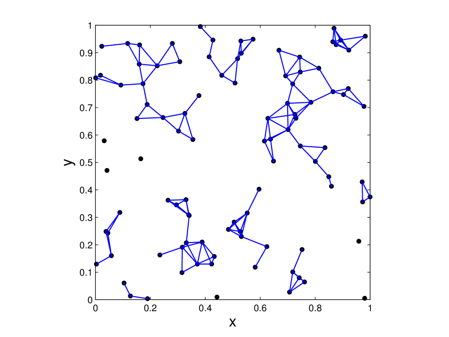
Figure 1: Proximity graph for $100$ vertices and radius $r=0.05$.

We illustrate the approach with an example. Fix a convex region $A\subset{\mathbb{R}}^{d}$ and let ${\mathcal{V}}\subset A$ be a finite set of $p$ points. For each number $r\geq 0$, the proximity graph $\mbox{Prox}({\mathcal{V}},r)$ (see Figure 1) is formed by joining every pair of (unordered) elements in ${\mathcal{V}}$ whose distance is $2r$ or less, i.e., whose closed balls of radius $r$ intersect. As $r$ ranges from $0$ to half the diameter of $A$, the graph $\mbox{Prox}({\mathcal{V}},r)$ ranges from the totally disconnected graph to the complete graph. This example is a particular case of a more general construction illustrated in Figure 2; hypergraphs can be computed from properties of intersections of classes of convex subsets in Euclidean space. The convex sets we consider are subsets of ${\mathbb{R}}^{d}$ that are simple to parametrize and compute. The key concept in our construction is the nerve:

Definition 2.1 (Nerve).

Let $F=\left\{A_{j},\ j\in I\right\}$ be a finite collection of distinct nonempty convex sets. The nerve of $F$ is given by

$$\textrm{Nrv}(F)=\left\{\sigma\subseteq I:\bigcap_{j\in\sigma}A_{j}\neq\varnothing\right\}.$$

The nerve of a family of sets uniquely determines a hypergraph. We use the following three nerves in this paper to construct hypergraphs (for more details, see Edelsbrunner and Harer, 2008).

Definition 2.2 (Čech Complex).

Let ${\mathcal{V}}$ be a finite set of points in ${\mathbb{R}}^{d}$ and $r>0$. Denote by ${\mathbb{B}^{d}}$ the closed unit ball in ${\mathbb{R}}^{d}$. The Čech complex corresponding to ${\mathcal{V}}$ and $r$ is the nerve of the sets $B_{v,r}=v+r{\mathbb{B}^{d}}$, $v\in{\mathcal{V}}$. This is denoted by $\textrm{Nrv}({\mathcal{V}},r,\textrm{\v{C}ech})$.

Definition 2.3 (Delaunay Triangulation).

Let ${\mathcal{V}}$ be a finite set of points in ${\mathbb{R}}^{d}$. The Delaunay triangulation corresponding to ${\mathcal{V}}$ is the nerve of the sets $C_{v}=\left\{x\in{\mathbb{R}}^{d}:~{}\|x-v\|\leq\|x-u\|,\ u\in{\mathcal{V}}\right\}$ for $v\in{\mathcal{V}}$. This is denoted by $\textrm{Nrv}({\mathcal{V}},\text{Delaunay})$, and the sets $C_{v}$ are called Voronoi cells.

Definition 2.4 (Alpha Complex).

Let ${\mathcal{V}}$ be a finite set of points in ${\mathbb{R}}^{d}$ and $r>0$. The Alpha complex corresponding to ${\mathcal{V}}$ and $r$ is the nerve of the sets $B_{v,r}\cap C_{v}$, $v\in{\mathcal{V}}$. This is denoted by $\textrm{Nrv}({\mathcal{V}},r,\textrm{Alpha})$.

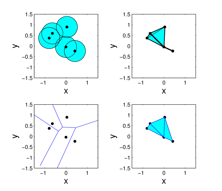
Figure 2: (a) A set of vertices in ${\mathbb{R}}^{2}$ are used to construct a family of disks of radius $r=0.5$. (b) The nerve of this convex set. This is an example of a Čech complex. (c) For the same vertex set the Voronoi diagram is computed. (d) The nerve of the Voronoi cells is obtained. This is an example of the Delaunay triangulation. Note that the maximum clique size of the Delaunay is bounded by the dimension of the space of the vertex set plus one; such a restriction does not apply to the Čech complex.

Here we illustrate the idea of nerve and specifically, the idea of alpha complex. Consider the vertex set displayed in Table 1 and $r=0.5$. The sets $B_{v,r}\cap C_{v}$ and the corresponding nerve (alpha complex) are illustrated in Figure 3. Since the set indexed by $V_{4}$ does not intersect with any other $B_{v,r}\cap C_{v}$, it will produce an isolated vertex in the nerve. The set indexed by $V_{1}$ only intersects with the set indexed by $V_{2}$, therefore there will be an edge joining $V_{1}$ and $V_{2}$ in the nerve. $V_{2}$, $V_{3}$ and $V_{5}$ intersect as pairs, therefore, the edges of the triangle with vertices $V_{2}$, $V_{3}$ and $V_{5}$ will be in the nerve. Since the sets indexed by $V_{2}$, $V_{3}$ and $V_{5}$ also intersect as a triad, the facet or face of the triangle is also included in the nerve.

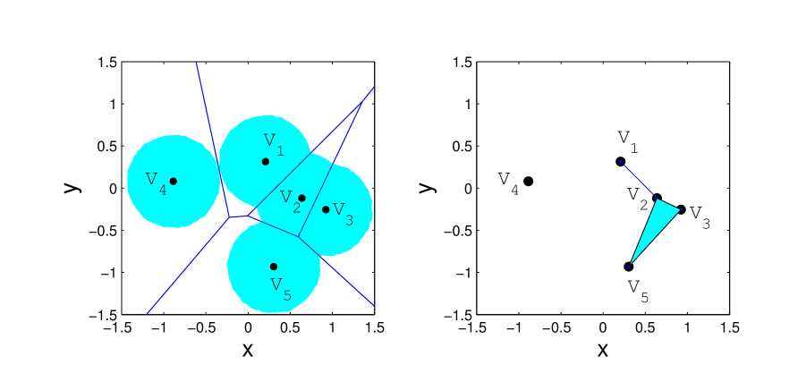
Figure 3: (a) Intersection of balls and Voronoi cells computed using $r=0.5$ and the vertex set listed in Table 1. (b) The corresponding Alpha complex.

Coordinate	$V_{1}{}$	$V_{2}{}$	$V_{3}{}$	$V_{4}{}$	$V_{5}{}$
$x$	$0.2065$	$0.6383$	$0.9225$	$-0.8863$	$0.3043$
$y$	$0.3149$	$-0.1193$	$-0.2544$	$0.0816$	$-0.9310$

Table 1: Vertex set used for generating a family of sets and the corresponding nerve.

The nerve of a family of sets is a particular class of hypergraphs known as (abstract) simplicial complexes.

Definition 2.5 (Abstract simplicial complex).

Let ${\mathcal{V}}$ be a finite set. A simplicial complex with base set ${\mathcal{V}}$ is a family ${\mathcal{K}}$ of subsets of ${\mathcal{V}}$ such that $\tau\in{\mathcal{K}}$ and $\sigma\subseteq\tau$ implies $\sigma\in{\mathcal{K}}$. The elements of ${\mathcal{K}}$ are called simplices, and the number of connected components of ${\mathcal{K}}$ is denoted $\sharp({\mathcal{K}})$.

The nerve of a collection of sets is always a hypergraph; in simple cases, only vertex pairs arise so the $1$-skeleton determines a unique graph.

Definition 2.6 ($p$-skeleton).

Let ${\mathcal{K}}$ be a simplicial complex, and denote by $|\tau|$ the cardinality of a simplex $\tau\in{\mathcal{K}}$. The $p$-skeleton of ${\mathcal{K}}$ is the collection of all $\tau\in{\mathcal{K}}$ such that $|\tau|\leq p+1$. The elements of the $p$-skeleton are called $p$-simplices and the $1$-skeleton is just a graph (more precisely, it is ${\mathcal{V}}\cup{\mathcal{E}}$ for a uniquely determined graph ${\mathcal{G}}=({\mathcal{V}},{\mathcal{E}})$).

The $1$-skeleton of a nerve is the graph obtained by considering only nonempty pairwise intersections. The process of obtaining the nerve and the $1$-skeleton from a family of sets is illustrated in Figure 4. Different families of convex sets in ${\mathbb{R}}^{d}$ induce different restrictions in graph space: for the Delaunay triangulation and the Alpha complex, for example, clique sizes cannot exceed $d+1$. Although no such blanket restriction applies to the Čech complex, for this complex some graphs are still unattainable— for example, no Čech complex can include a star graph whose central node has degree higher than the “kissing number,” i.e., maximal number of disjoint unit hyperspheres touching a given hypersphere, 6 for $d=2$, 12 for $d=3$, etc.

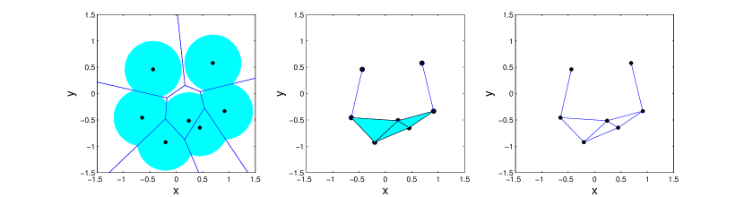
Figure 4: (a) Given a set of vertices and a radius ($r=0.5$) one can compute $A_{i}=C_{i}\cap B_{i}$, where $C_{i}$ is the Voronoi cell for vertex $i$ and $B_{i}$ is the ball of radius $r$ centered at vertex $i$. (b) The Alpha complex is the nerve of the $A_{i}$’s. (c) Often the main interest will be the $1$-skeleton of the complex, which is the subset of the nerve that corresponds to (nonempty) pairwise intersections.

The Čech and Alpha complexes are hypergraphs indexed by a finite set ${\mathcal{V}}=\left\{V_{1},\ldots,V_{p}\right\}\subset{\mathbb{R}}^{d}$ and a size parameter $r\geq 0$. Each induces a parametrization on the space of hypergraphs $({\mathcal{V}},r)\mapsto{\mathcal{H}}({\mathcal{V}},r)$. The class ${\mathcal{A}}$ of convex sets used to compute the nerve determines the space of hypergraphs. To keep the notation simple, ${\mathcal{A}}$ will be implicit whenever obvious by the context. We will use $A({\mathcal{V}},r)$ to denote a generic element of ${\mathcal{A}}$ for either the Čech or the Alpha complex. Similarly, $1$-skeletons of nerves induce a parametrization of the spaces of graphs $({\mathcal{V}},r)\mapsto{\mathcal{G}}({\mathcal{V}},r)$.

Two principal advantages of this approach are:

1. For each family of convex sets $\left\{{\mathcal{A}}\right\}$, the number of parameters needed to specify the graph ${\mathcal{G}}$ or hypergraph ${\mathcal{H}}$ grows only linearly with the number of vertices;

2. The hypergraph parameter space will be a subset of ${\mathbb{R}}^{d}$, a very convenient parameter space for MCMC sampling.

2.3 Random geometric graphs

In Section 2.2 we demonstrated how the geometry of a set ${\mathcal{V}}$ of $p$ points in ${\mathbb{R}}^{d}$ can be used to induce a graph ${\mathcal{G}}$. In this section we explore the relation between prior distributions on random sets ${\mathbf{V}}$ of points in ${\mathbb{R}}^{d}$ and features of the induced distribution on graphs ${\mathcal{G}}$, with the goal of learning how to tailor a point process model to obtain graph distributions with desired features.

Definition 2.7 (Random Geometric Graph).

Fix integers $p,d\in{\mathbb{N}}$ and let ${\mathbf{V}}=(V_{1},\ldots,V_{p})$ be drawn from a probability distribution ${\mathcal{Q}}$ on $({\mathbb{R}}^{d})^{p}$. For any class ${\mathcal{A}}$ of convex sets in ${\mathbb{R}}^{d}$ and radius $r>0$, the graph ${\mathcal{G}}({\mathbf{V}},r,{\mathcal{A}})$ is said to be a Random Geometric Graph (RGG).

While Definition 2.7 is more general than that of (Penrose, 2003, p. 2), it still cannot describe all the random graphs discussed in (Penrose and Yukich, 2001) (for example, those based on $k$-neighbors cannot in general be generated by nerves). For ${\mathcal{A}}$ we will use closed balls in ${\mathbb{R}}^{d}$ or intersections of balls and Voronoi cells; most often ${\mathcal{Q}}$ will be a product measure under which the $\left\{V_{i}\right\}$ will be $p$ independent identically distributed (iid) draws from some marginal distribution ${\mathcal{Q}}_{M}$ on ${\mathbb{R}}^{d}$, such as the uniform distribution on the unit cube $[0,1]^{d}$ or unit ball ${\mathbb{B}^{d}}$, but we will also explore the use of repulsive processes for ${\mathbf{V}}$ under which the points $\left\{V_{i}\right\}$ are more widely dispersed than under independence. It is clear that different choices for ${\mathcal{A}}$, ${\mathcal{Q}}$ and $r$ will have an impact on the support of the induced RGG distribution. To make this notion precise we define feasible graphs.

Definition 2.8 (Isomorphic).

Write ${\mathcal{G}}_{1}\cong{\mathcal{G}}_{2}$ for two graphs ${\mathcal{G}}_{i}=({\mathcal{V}}_{i},{\mathcal{E}}_{i})$ and call the graphs isomorphic if there is a 1:1 mapping $\chi:{\mathcal{V}}_{1}\to{\mathcal{V}}_{2}$ such that $\left(v_{i},v_{j}\right)\in{\mathcal{E}}_{1}\Leftrightarrow\left(\vrule width=0.0pt,height=10.0pt,depth=0.0pt\chi(v_{i}),\chi(v_{j})\right)\in{\mathcal{E}}_{2}$ for all $v_{i},v_{j}\in{\mathcal{V}}_{1}$.

Definition 2.9 (Feasible Graph).

Fix numbers $d,p\in{\mathbb{N}}$, a class ${\mathcal{A}}$ of convex sets in ${\mathbb{R}}^{d}$, and a distribution ${\mathcal{Q}}$ on the random vectors ${\mathbf{V}}$ in $({\mathbb{R}}^{d})^{p}$. A graph $\Gamma$ is said to be feasible if for some number $r>0$,

$$\Pr\left\{{\mathcal{G}}({\mathbf{V}},r,{\mathcal{A}})\cong\Gamma\right\}>0.$$

In contrast to Erdös-Rényi models, where the inclusion of graph edges are independent events, the RGG models exhibit edge dependence that depends on the metric structure of ${\mathbb{R}}^{d}$ and the class ${\mathcal{A}}$ of convex sets used to construct the nerves.

There is an extensive literature describing asymptotic distributions for a variety of graph features such as: subgraph counts, vertex degree, order of the largest clique, and maximum vertex degree (for an encyclopedic account of results for the important case of $1$-skeletons of Čech complexes, see Penrose, 2003). Several results for the Delaunay triangulation, some of which generalize to the Alpha complex, are reported in (Penrose and Yukich, 2001). Regarding the support on the distribution of hypergraphs induced by the complexes, generally, this is an area of open research (personal communication with H. Edelsbrunner). Recent work by Kalhe (2014) surveys some of this literature, focusing on random simplicial complexes. The monograph by Penrose (2003) discusses the relationship between ${\mathcal{Q}}$ and subgraph counts, the degree distribution, and the percolation threshold, in Chapters 3, 4 and 10, respectively

Penrose (2003, Chap. 3) gives conditions which guarantee the asymptotic normality of the joint distribution of the numbers $Q_{j}$ of $j$-simplices (edges, triads, etc.), for iid samples ${\mathbf{V}}=(V_{1},\ldots,V_{p})$ from some marginal distribution ${\mathcal{Q}}_{M}$ on ${\mathbb{R}}^{d}$, as the number $p=|{\mathbf{V}}|$ of vertices grows and the radius $r_{p}$ shrinks.

Simulation studies suggest that the asymptotic results apply approximately for $p\geq 24$–$100$. By this we mean that sometimes $24$ is sufficient (the distribution of the vertices is approximately multivariate normal), and sometimes $100$ may be required (distribution of the vertices far from being multivariate normal).

3 Geometric representations of random hypergraphs

We develop a Bayesian approach to the problem of inferring factorizations of distributions of the forms of (2.1),

$$f(x)=\prod_{a\in{\mathscr{C}}({\mathcal{G}})}\phi_{a}(x_{a}\mid\theta_{a})\text{\quad or\quad}\frac{\prod_{a\in{\mathscr{P}}({\mathcal{G}})}\psi_{a}(x_{a}\mid\theta_{a})}{\prod_{b\in{\mathscr{S}}({\mathcal{G}})}\psi_{b}(x_{b}\mid\theta_{b})}.$$

In each case we specify the prior density function as a product

$$p(\theta,{\mathcal{G}})=p(\theta\mid{\mathcal{G}})\,p({\mathcal{G}})$$ (3.1)

of a conditional hyper Markov law for $\theta\in\Theta$ and a marginal RGG law on ${\mathcal{G}}$. We use conventional methods to select the specific hyper Markov distribution (hyper Inverse Wishart for multivariate normal sampling distributions, for example) since our principal focus is on prior distributions for the graphs, $p({\mathcal{G}})$. Every time we refers to hyper Markov laws, it will be in the strong sense according to Dawid and Lauritzen (1993). We also present MCMC algorithms for sampling from the posterior distribution on ${\mathcal{G}}$, for observed data.

3.1 Prior specifications

All the graphs in our statistical models are built from nerves constructed in Section 2.2 from a random vertex set ${\mathcal{V}}=\left\{V_{i}\right\}_{i=1}^{p}\subset{\mathbb{R}}^{d}$ and radius $r>0$. Since the nerve construction is invariant under rigid transformations (this is, transformations that preserve angles as well as distances) of ${\mathcal{V}}$ or simultaneous scale changes in ${\mathcal{V}}$ and $r$, restricting the support of the prior distribution on ${\mathcal{V}}$ to the unit ball ${\mathbb{B}^{d}}$ does not reduce the model space:

Proposition 3.1.

Every feasible graph in ${\mathbb{R}}^{d}$ may be represented in the form ${\mathcal{G}}({\mathcal{V}},r,{\mathcal{A}})$ for a collection ${\mathcal{V}}$ of $p$ points in the unit ball ${\mathbb{B}^{d}}$ and for $r={\frac{1}{p}}$.

Proof.

Let ${\mathcal{G}}=({\mathcal{V}},{\mathcal{E}})\cong{\mathcal{G}}({\mathcal{V}},r,{\mathcal{A}})$ be a feasible graph with $|{\mathcal{V}}|=p$ vertices. Every edge $\left(v_{i},v_{j}\right)\in{\mathcal{E}}$ has length ${\textrm{dist}\left(v_{i},v_{j}\right)}\leq 2r$ so, by the triangle inequality, every connected component $\Gamma_{i}$ of ${\mathcal{G}}$ with $p_{i}$ vertices must have diameter no greater than the longest possible path length, $2r(p_{i}-1)$, and so fits in a ball $B_{i}$ of diameter $2r(p_{i}-1)$. The union of these balls, centered on a line segment and separated by $r(2+1/p)$, will have diameter less than $r(2p-1)$. By translation and linear rescaling we may take $r=1/p$ and bound the diameter by $2$, completing the proof. ∎

We fix $r={\frac{1}{p}}$ and simplify the notation by writing ${\mathcal{G}}({\mathcal{V}},{\mathcal{A}})$ instead of ${\mathcal{G}}({\mathcal{V}},r,{\mathcal{A}})$ for ${\mathcal{A}}=\textrm{\v{C}ech}$ or ${\mathcal{A}}=\textrm{Alpha}$ or, if ${\mathcal{A}}$ is understood, simply ${\mathcal{G}}({\mathcal{V}})$. Thus we can induce prior distributions on the space of feasible graphs from distributions on configurations of $p$ points in the unit ball in ${\mathbb{R}}^{d}$.

For iid uniform draws ${\mathbf{V}}=(V_{1},\dots,V_{p})$ from ${\mathbb{B}^{d}}$, the expected number of edges of the graph ${\mathcal{G}}({\mathbf{V}},r,{\mathcal{A}})$ is bounded above by $\mathcal{E}[\#{\mathcal{E}}]\leq\binom{n}{2}(2r)^{d}$; for $r={\frac{1}{p}}$ in dimension $d=2$ this is less than $\mathcal{E}[\#{\mathcal{E}}]<2$, leading to relatively sparse graphs. We often take larger values of $r$ (still small enough for empty graphs to be feasible), to generate richer classes of graphs. A limit to how large $r$ may be is given by the partial converse to Prop. 3.1,

Proposition 3.2.

The empty graph on $p$ vertices cannot be expressed as ${\mathcal{G}}({\mathcal{V}},r,\textrm{\v{C}ech})$ for any ${\mathcal{V}}\subset{\mathbb{B}^{d}}$ with $r\geq\big{(}p^{1/d}-1\big{)}^{-1}$.

Proof.

Let ${\mathcal{V}}=\left\{V_{1},\dots,V_{p}\right\}\subset{\mathbb{B}^{d}}$ be a set of points and $r>0$ a radius such that ${\mathcal{G}}({\mathcal{V}},r,\textrm{\v{C}ech})$ is the empty graph. Then the balls ${\mathcal{V}}_{i}+r{\mathbb{B}^{d}}$ are disjoint and their union with $d$-dimensional volume $p\omega_{d}r^{d}$ lies wholly within the ball $(1+r){\mathbb{B}^{d}}$ of volume $\omega_{d}(1+r)^{d}$ (where $\omega_{d}=\pi^{d/2}/\Gamma(1{+}d/2)$ is the volume of the unit ball), so $p<(1+\frac{1}{r})^{d}$. ∎

Slightly stronger, the empty graph may not be attained as ${\mathcal{G}}({\mathcal{V}},r,\textrm{\v{C}ech})$ for any $r\geq 1/[(p/p_{d})^{1/d}-1]$ where $p_{d}$ is the maximum spherical packing density in ${\mathbb{R}}^{d}$. For $d=2$, this gives the asymptotically sharp bound $r<1\Big{/}\Big{[}\sqrt{p\sqrt{12}/\pi}-1\Big{]}$.

3.2 Sampling from prior and posterior distributions

Let ${\mathcal{Q}}$ be a probability distribution on $p$-tuples in ${\mathbb{R}}^{d}$, $p({\mathcal{G}})$ the induced prior distribution on graphs ${\mathcal{G}}({\mathbf{V}},\textrm{\v{C}ech})$ for ${\mathbf{V}}\sim{\mathcal{Q}}$ with $r={\frac{1}{p}}$, and let $p(\theta\mid{\mathcal{G}})$ be a conventional hyper Markov law (see below). We wish to draw samples from the prior distribution $p(\theta,{\mathcal{G}})$ of (3.1) and from the posterior distribution $p(\theta,{\mathcal{G}}\mid{\mathbf{x}})$, given a vector ${\mathbf{x}}=(x_{1},...,x_{m})$ of iid observations $x_{j}\mathrel{\mathop{\sim}\limits^{\mathrm{iid}}}f(x\mid\theta)$, using the Metropolis/Hastings approach to MCMC (Hastings, 1970; Robert and Casella, 2004, Ch. 7).

We begin with a random walk proposal distribution in ${\mathbb{B}^{d}}$ starting at an arbitrary point $v\in{\mathbb{B}^{d}}$, that approximates the steps $\left\{V^{(0)},V^{(1)},V^{(2)},...\right\}$ of a diffusion $V^{(t)}$ on ${\mathbb{B}^{d}}$ with uniform stationary distribution and reflecting boundary conditions at the unit sphere $\partial{\mathbb{B}^{d}}$.

The random walk is conveniently parametrized in spherical coordinates with radius $\rho^{(t)}=\parallel V^{(t)}\parallel$ and Euler angles— in $d{=}2$ dimensions, angle $\varphi^{(t)}$— at step $t$. Informally, we take independent radial random walk steps such that $(\rho^{(t)})^{d}$ is reflecting Brownian motion on the unit interval (this ensures that the stationary distribution will be $\textsf{Un}({\mathbb{B}^{d}})$) and, conditional on the radius, angular steps from Brownian motion on the $d$-sphere of radius $\rho^{(t)}$.

Fix some $\eta>0$. In $d=2$ dimensions the reflecting random walk proposal $(\rho^{*},\varphi^{*})$ we used for step $(t+1)$, beginning at $(\rho^{(t)},\varphi^{(t)})$, is:

$$\rho^{*}=R\Big{(}[\rho^{(t)}]^{2}+\zeta_{\rho}^{(t)}\,\eta\Big{)}^{1/2},\qquad\varphi^{*}=\varphi^{(t)}+\zeta_{\phi}^{(t)}\,\eta/\rho^{(t)}$$

for iid standard normal random variables $\left\{\zeta_{\rho}^{(t)},\zeta_{\phi}^{(t)}\right\}$, where

$$R(x)=\left|x-2\left\lfloor{\textstyle\frac{1}{2}}(x+1)\right\rfloor\right|$$

is $x$ reflected (as many times as necessary) to the unit interval. Similar expressions work in any dimension $d$, with $\rho^{*}=R\Big{(}[\rho^{(t)}]^{d}+\zeta_{\rho}^{(t)}\,\eta\Big{)}^{1/d}$ and appropriate step sizes for the $(d-1)$ Euler angles.

For small $\eta>0$ this diffusion-inspired random walk generates local moves under which the proposed new point $(\rho^{*},\varphi^{*})$ is quite close to $(\rho^{(t)},\varphi^{(t)})$ with high probability. To help escape local modes, and to simplify the proof of ergodicity below, we add the option of more dramatic “global” moves by introducing at each time step a small probability of replacing $(\rho^{(t)},\varphi^{(t)})$ with a random draw $(\rho^{*},\varphi^{*})$ from the uniform distribution on ${\mathbb{B}^{d}}$ (see Figure 5). Let $q({\mathcal{V}}^{*}\mid{\mathcal{V}})$ denote the Lebesgue density at ${\mathcal{V}}^{*}\in({\mathbb{B}^{d}})^{p}$ of one step of this hybrid random walk for ${\mathcal{V}}=(V_{1},\dots,V_{p})$, starting at ${\mathcal{V}}\in({\mathbb{B}^{d}})^{p}$.

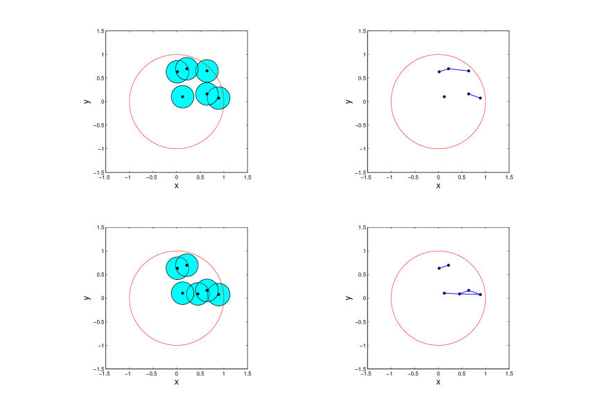
Figure 5: This figure illustrates a global move. (a) The current configuration of the points. (b) The graph implied by this configuration. (c) The proposal configuration which is obtained by randomly moving one vertex. (d) The graph implied by the proposed move.

3.2.1 Prior sampling

To draw sample graphs from the prior distribution begin with ${\mathbf{V}}^{(0)}\sim{\mathcal{Q}}(d{\mathbf{V}})$ and, after each time step $t\geq 0$, propose a new move to ${\mathbf{V}}^{*}\sim q({\mathbf{V}}^{*}\mid{\mathbf{V}}^{(t)})$. The proposed move from ${\mathbf{V}}^{(t)}$ (with induced graph ${\mathcal{G}}^{(t)}={\mathcal{G}}({\mathbf{V}}^{(t)})$) to ${\mathbf{V}}^{*}$ (and ${\mathcal{G}}^{*}$) is accepted (whereupon ${\mathbf{V}}^{(t+1)}={\mathbf{V}}^{*}$) with probability $1\wedge H^{(t)}$, the minimum of one and the Metropolis/Hastings ratio

$$H^{(t)}=\frac{p({\mathbf{V}}^{*})~{}~{}q({\mathbf{V}}^{(t)}\mid{\mathbf{V}}^{*})}{p({\mathbf{V}}^{(t)})~{}q({\mathbf{V}}^{*}\mid{\mathbf{V}}^{(t)})}.$$

Otherwise ${\mathbf{V}}^{(t+1)}={\mathbf{V}}^{(t)}$; in either case set $t\leftarrow t{+}1$ and repeat. Note the proposal distribution $q(\cdot\mid\cdot)$ leaves the uniform distribution invariant, so $H^{(t)}\equiv 1$ for ${\mathcal{Q}}(d{\mathbf{V}})\propto d{\mathbf{V}}$ and in that case every proposal is accepted.

3.2.2 Posterior sampling

After observing a random sample $X={\mathbf{x}}=(x_{1},\dots,x_{m})$ from the distribution $x_{j}\sim f(x\mid\theta,{\mathcal{G}})$, let

$$f({\mathbf{x}}\mid\theta,{\mathcal{G}}) =\prod_{i=1}^{m}f(x_{i}\mid\theta,{\mathcal{G}})$$

denote the likelihood function and

$${\mathcal{M}}({\mathcal{G}}) =\int_{\Theta_{\mathcal{G}}}f({\mathbf{x}}\mid\theta,{\mathcal{G}})\,p(\theta\mid{\mathcal{G}})d\theta$$ (3.2)

the marginal likelihood for $${\mathcal{G}} {\mathbf{V}}^{(t)} {\mathbf{V}}^{*} 1\wedge H^{(t)}$$. For posterior sampling of graphs, a proposed move from to is accepted with probability for

$$H^{(t)} =\frac{{\mathcal{M}}({\mathcal{G}}^{*})~{}p({\mathbf{V}}^{*})~{}~{}q({\mathbf{V}}^{(t)}\mid{\mathbf{V}}^{*})}{{\mathcal{M}}({\mathcal{G}}^{(t)})~{}p({\mathbf{V}}^{(t)})~{}q({\mathbf{V}}^{*}\mid{\mathbf{V}}^{(t)})}.$$ (3.3)

For multivariate normal data $X$ and hyper inverse Wishart hyper Markov law $p(\theta\mid{\mathcal{G}})$, ${\mathcal{M}}({\mathcal{G}})$ from (3.2) can be expressed in closed form for decomposable graphs ${\mathcal{G}}({\mathbf{V}})$. efficient algorithms for evaluating (3.2) are still available even if this condition fails.

The model will typically be of variable dimension, since the parameter space $\Theta_{\mathcal{G}}$ for the factors may depend on the graph ${\mathcal{G}}={\mathcal{G}}({\mathbf{V}})$. Not all proposed moves of the point configuration ${\mathbf{V}}^{(t)}\rightsquigarrow{\mathbf{V}}^{*}$ will lead to a change in ${\mathcal{G}}({\mathbf{V}})$; for those that do we implement reversible-jump MCMC (Green, 1995; Sisson, 2005) using the auxiliary variable approach of Brooks et al. (2003) to simplify the book-keeping needed for non-nested moves $\Theta_{\mathcal{G}}\rightsquigarrow\Theta_{{\mathcal{G}}^{*}}$.

3.3 Convergence of the Markov chain

Denote by $\dot{{\mathcal{G}}}(p,d,{\mathcal{A}})$ the finite set of feasible graphs with $p$ vertices in ${\mathbb{R}}^{d}$, i.e., those generated from $1$-skeletons of ${\mathcal{A}}$-complexes. For each ${\mathcal{G}}\in\dot{{\mathcal{G}}}(p,d,{\mathcal{A}})$ let $V_{\mathcal{G}}\subset({\mathbb{B}^{d}})^{p}$ denote the set of all points ${\mathbf{V}}=\left\{V_{1},\dots,V_{p}\right\}\in({\mathbb{B}^{d}})^{p}$ for which ${\mathcal{G}}\cong{\mathcal{G}}({\mathbf{V}},{\frac{1}{p}},{\mathcal{A}})$, and set $\mu({\mathcal{G}})={\mathcal{Q}}\big{(}V_{\mathcal{G}}\big{)}$. Then

Proposition 3.3.

The sequence ${\mathcal{G}}^{(t)}={\mathcal{G}}({\mathbf{V}}^{(t)},{\frac{1}{p}},{\mathcal{A}})$ induced by the prior MCMC procedure described in Section 3.2.1 samples each feasible graph ${\mathcal{G}}\in\dot{{\mathcal{G}}}(p,d,{\mathcal{A}})$ with asymptotic frequency $\mu({\mathcal{G}})$. The posterior procedure described in Section 3.2.2 samples each feasible graph with asymptotic frequency $\mu({\mathcal{G}}\mid{\mathbf{x}})$, the posterior distribution of ${\mathcal{G}}$ given the data ${\mathbf{x}}$ and hyper Markov prior $p(\theta\mid{\mathcal{G}})$.

Proof.

Both statements follow from the Harris recurrence of the Markov chain ${\mathbf{V}}^{(t)}$ constructed in Section 3.2. For this it is enough to find a strictly positive lower bound for the probability of transitioning from an arbitrary point $V\in({\mathbb{B}^{d}})^{p}$ to any open neighborhood of another arbitrary point $V^{*}\in({\mathbb{B}^{d}})^{p}$ (Robert and Casella, 2004, Theorem 6.38, pg. 225). This follows immediately from our inclusion of the global move in which all $p$ points $\left\{V_{i}\right\}$ are replaced with uniform draws from $({\mathbb{B}^{d}})^{p}$. ∎

It is interesting to note that while the sequence ${\mathcal{G}}^{(t)}={\mathcal{G}}({\mathbf{V}}^{(t)},{\frac{1}{p}},{\mathcal{A}})$ is a hidden Markov process, it is not itself Markovian on the finite state space $\dot{{\mathcal{G}}}(p,d,{\mathcal{A}})$; nevertheless it is ergodic, by Prop. 3.3.

4 Results

Here we illustrate the use of the proposed parametrization using simulations and real data. These numerical examples provide us with an opportunity to test priors that encourage sparsity, and MCMC algorithms that allow for local as well as global moves by design.

4.1 Illustration of modeling advantages

4.1.1 The nerve determines the junction tree factorization

Here we use a junction tree factorization with each univariate marginal $X_{i}$ associated to a point $V_{i}\in{\mathbb{R}}^{d}$ (the standard graphical models approach). In this case, specifying the class of sets to compute the nerve and the value for $r$ determines a factorization for the joint density of $\left\{X_{1},\ldots,X_{p}\right\}$. We illustrate with $p=5$ points in Euclidean space of dimension $d=2$.

Let $(X_{1},X_{2},X_{3},X_{4},X_{5})\in{\mathbb{R}}^{2}$ be a random vector with density $f(x)$ and consider the vertex set displayed in Table 1 (also shown as solid dots in Figures 3 and 6).

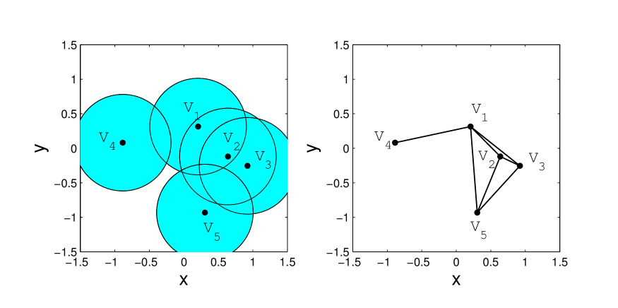
Figure 6: (a) Čech complex computed using $r=0.7$ and the vertex set listed in Table 1. (b) The $1$-Skeleton of the Čech complex.

For an Alpha complex with $r=0.5$ the junction tree factorization (2.1b) corresponding to the graph in Figure 3 is

$$f(x)=\frac{\psi_{12}(x_{1},x_{2})\psi_{235}(x_{2},x_{3},x_{5})\psi_{4}(x_{4})}{\psi_{2}(x_{2})},$$

we will denote the factorization as $[1,2][2,3,5][4]$. In the case where the factors are potential functions rather than marginals we will use $\{\cdot\}$ instead of $[\cdot]$. Similarly, for the Čech complex and $r=0.7$ the factorization corresponding to the graph in Figure 6 is

$$f(x)=\frac{\psi_{1235}(x_{1},x_{2},x_{3},x_{5})\psi_{14}(x_{1},x_{4})}{\psi_{1}(x_{1})}.$$

4.1.2 Subgraph counts in RGGs are a function of ${\mathcal{Q}}$

In this subsection we illustrate how the distribution of particular graph features changes as a function of the sampling distribution of the random point set ${\mathbf{V}}$ and contrast this with Erdös-Rényi models. Specifically we will focus on the number of edges (2-cliques) $Q_{2}$ and the number of 3-cliques $Q_{3}$.

The two spatial processes we study for ${\mathcal{Q}}$ are iid uniform draws from the unit square $[0,1]^{2}$ in the plane, and dependent draws from the Matérn type III hard-core repulsive process (Huber and Wolpert, 2009), using Čech complexes with radius $r=1/\sqrt{150}\approx 0.082$ in both cases to ensure asymptotic normality (Penrose, 2003, Thm. 3.13). In our simulations we vary both the number of variables (graph size) $p$ and the Matérn III hard core radius $\rho$. Comparisons are made with an Erdös-Rényi model with a common edge inclusion parameter. Table 2 displays the quartiles for $Q_{2}$ and $Q_{3}$ as a function of the graph size $p$, hard core radius $\rho$, and Erdös-Rényi edge inclusion probability $p$. Figures 7, 8, and 9 show the joint distribution of $(Q_{2},~{}Q_{3})$ for $\left\{V_{i}\right\}\mathrel{\mathop{\sim}\limits^{\mathrm{iid}}}\textsf{Un}([0,1]^{2})$, for a Matérn III process with hard core radius $\rho=0.35$, and for draws from an Erdös-Rényi model with inclusion probability $\alpha=0.065$, respectively.

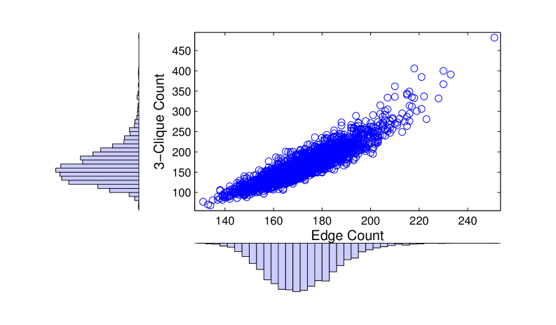
Figure 7: Edge counts and $3$-Clique counts from $2,500$ simulated samples of ${\mathcal{G}}({\mathbf{V}},1/\sqrt{2\cdot 75},\textrm{\v{C}ech})$ where $|{\mathbf{V}}|=75$ and $V_{i}\mathrel{\mathop{\sim}\limits^{\mathrm{iid}}}\textsf{Un}([0,1]^{2})$, $1\leq i\leq 75$. The multivariate normal appears as a reasonable approximation for the joint distribution, as suggested by (Penrose, 2003, Thm. $3.13$). Čech radius is $r_{n}=1/\sqrt{2n}$.

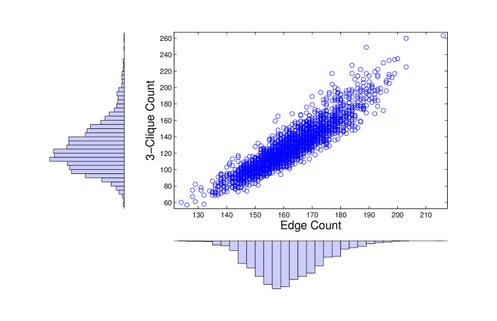
Figure 8: Edge counts and $3$-Clique counts from $2,500$ simulated samples of ${\mathcal{G}}({\mathbf{V}},1/\sqrt{2\cdot 75},\textrm{\v{C}ech})$ where $|{\mathbf{V}}|=75$ and $V$ sampled from a Mattérn III with hard-core radius $r=0.35$.

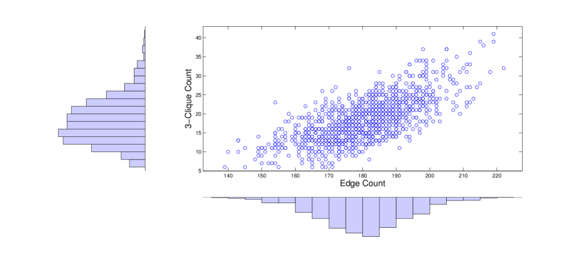
Figure 9: Edge counts and $3$-Clique counts from $1\,000$ simulated samples of an Erdös-Rényi graph with edge inclusion probability of $p=0.065$.

Graph		$|{\mathcal{V}}|$	Edges			$3$-Cliques
			$25\%$	$50\%$	$75\%$	$25\%$	$50\%$	$75\%$
Uniform		$75$	$161$	$171$	$182$	$134$	$160$	$190$
Matérn	$(0.035)$	$75$	$154$	$161$	$170$	$110$	$124$	$144$
ER	$(0.050)$	$75$	$130$	$138$	$146$	$6$	$8$	$11$
ER	$(0.065)$	$75$	$172$	$181$	$189$	$14$	$18$	$22$
Uniform		$50$	$69$	$75$	$81$	$34$	$43$	$57$
Matérn	$(0.035)$	$50$	$66$	$71$	$76$	$27$	$35$	$43$
Matérn	$(0.050)$	$50$	$62$	$67$	$71$	$22$	$27$	$33$
ER	$(0.050)$	$50$	$56$	$61$	$67$	$1$	$2$	$4$
ER	$(0.065)$	$50$	$74$	$79$	$85$	$3$	$5$	$7$
Uniform		$20$	$9$	$12$	$14$	$1$	$2$	$4$
Matérn	$(0.035)$	$20$	$9$	$11$	$13$	$1$	$1$	$3$
Matérn	$(0.050)$	$20$	$8$	$10$	$12$	$0$	$1$	$2$
ER	$(0.050)$	$20$	$8$	$9$	$11$	$0$	$0$	$0$
ER	$(0.065)$	$20$	$10$	$12$	$15$	$0$	$0$	$1$

Table 2: Summaries of the empirical distribution of edge and $3$-clique counts for Čech complex random geometric graphs with radius $r=0.082$, for vertex sets sampled from iid draws from the unit square from: a uniform distribution, a hard core process with radius $\rho=0.035$, and from Erdös-Rényi (ER) with common edge inclusion probabilities of $\alpha=0.050$ and $\alpha=0.065$.

These simulations illustrate that by varying the distribution ${\mathcal{Q}}$ we can control the joint distribution of graph features. The repulsive and iid uniform distribution have very similar edge distributions, for example (see Figures 7 and 8), while (as anticipated) the repulsive process penalizes large cliques. Joint control of these features is not possible with an Erdös-Rényi model with a common edge inclusion probability and it is not obvious how to encode this type of information in the concordance function approach of Mukherjee and Speed (2008).

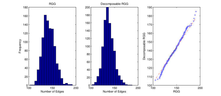
Figure 22: Distribution of edge counts for both unrestricted and decomposable graphs. Graphs were computed using Čech complex filtrations with $p=100$ and $V_{i}\mathrel{\mathop{\sim}\limits^{\mathrm{iid}}}\textsf{Un}([0,1]^{2})$.

In Section A we proposed a procedure for generating decomposable graphs, and noted that the graphs induced by this algorithm are similar to those constructed without the decomposability restriction. In Figure 22 we display a simulation study of the distribution of edge counts for a RGG and the restriction to decomposable graphs. These distributions are very similar.

4.2 Simulation studies

We develop four examples. The first example illustrates that our method works when the graph encoding the Markov structure of underlying density is contained in the space of graphs spanned by the nerve used to fit the model. In the second example we apply our method to Gaussian Graphical Models. The third example shows that the nerve hypergraph (not just the $1$-skeleton) can be used to induce different groupings in the terms of a factorization, and therefore a way to encode dependence features that go beyond pairwise relationships. In the fourth example we compare results obtained by using different filtrations to induce priors over different spaces of graphs.

4.2.1 ${\mathcal{G}}$ is in the Space Generated by ${\mathcal{A}}$

Let $\left(X_{1},\ldots,X_{10}\right)$ be a random vector whose distribution has factorization:

$$f_{\theta}({\mathbf{x}})=\frac{\psi_{\theta}(x_{1},x_{4},x_{10})\psi_{\theta}(x_{1},x_{8},x_{10})\psi_{\theta}(x_{4},x_{5})\psi_{\theta}(x_{8},x_{9})\psi_{\theta}(x_{2},x_{3},x_{9})\psi_{\theta}(x_{6})\psi_{\theta}(x_{7})}{\psi_{\theta}(x_{4})\psi_{\theta}(x_{8})\psi_{\theta}(x_{9})\psi_{\theta}(x_{1},x_{10})}$$ (4.1a)

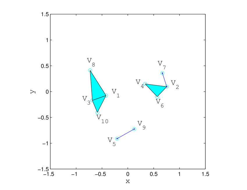
Figure 10: Geometric graph representing the model given in (4.1a). For this example graphs are constructed to be decomposable and the clique marginals are specified as Clayton copulas.

The Markov structure of (4.1a) can be encoded by the geometric graph displayed in Figure 10. We transform variables if necessary to achieve standard $\textsf{Un}(0,1)$ marginal distributions for each $X_{i}$, and model clique joint marginals with a Clayton copula Clayton, 1978, or Nelsen, 1999, §4.6, the exchangeable multivariate model with joint distribution function

$$\Psi_{\theta}({\mathbf{x}}_{I}) =\left(1-p_{I}+\sum_{i\in I}x_{i}^{-\theta}\right)^{-1/\theta}$$

and density function

$$\psi_{\theta}({\mathbf{x}}_{I}) =\theta^{p_{I}}~{}\frac{\Gamma(p_{I}+1/\theta)}{\Gamma(1/\theta)}\left(1-p_{I}+\sum_{i\in I}x_{i}^{-\theta}\right)^{-p_{I}-1/\theta}~{}\left(\prod_{i\in I}x_{i}\right)^{-1-\theta}$$ (4.1b)

on $[0,1]^{p_{I}}$ for some $\theta\in\Theta=(0,\infty)$, for each clique $[v_{i}:~{}i\in I]$ of size $p_{I}$.

We drew $250$ samples from model (4.1) with $\theta=4$. For inference about ${\mathcal{G}}$ we set ${\mathcal{A}}=\textrm{Alpha}$ and $r=0.30$, with independent uniform prior distributions for the vertices $V_{i}\mathrel{\mathop{\sim}\limits^{\mathrm{iid}}}\textsf{Un}({\mathbb{B}^{2}})$ on the unit ball in the plane. We used the random walk described in Section 3.2 to draw posterior samples with Algorithm 1 applied to enforce decomposability. To estimate $\theta$ we take a unit Exponential prior distribution $\theta\sim\textsf{Ex}(1)$ and employ a Metropolis/Hastings approach using a symmetric random walk proposal distribution with reflecting boundary conditions at $\theta=0$,

$$\theta^{*}=\big{|}\theta^{(t)}+\varepsilon\big{|},$$

with $\varepsilon_{t}\sim\textsf{Un}(-\beta,\beta)$ for fixed $\beta>0$. We drew $1\,000$ samples after a burn-in period of $25\,000$ draws. The three models with the highest posterior probabilities are displayed in Table 3. The geometric graphs computed from six posterior samples (one every $100$ draws) are shown in Figure 11; note that the computed nerves appear to stabilize after a few hundred iterations while the actual position of the vertex set continues to vary.

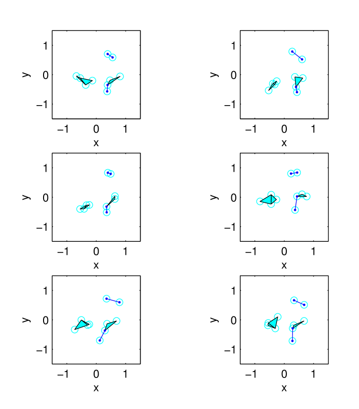
Figure 11: Geometric graphs corresponding to snapshots of posterior samples (one every 100 iterations) from model of (4.1a). For this example graphs are constructed to be decomposable and the clique marginals are specified as Clayton copulas.

Graph Topology	Posterior Probability
$\vrule width=0.0pt,height=10.0pt,depth=0.0pt{\color[rgb]{1,0,0}\bf[1,4,10]}{\color[rgb]{1,0,0}\bf[1,8,10]}{\color[rgb]{1,0,0}\bf[4,5]}{\color[rgb]{1,0,0}\bf[8,9]}{\color[rgb]{1,0,0}\bf[2,3,9]}{\color[rgb]{1,0,0}\bf[6]}{\color[rgb]{1,0,0}\bf[7]}$	$0.963$
$[1,4,10][1,8,10][4,5][8,9][2,3,9][6][5,7]$	$0.021$
$[1,4,10][1,8][4,5][8,9][2,3,9][6][7]$	$0.010$

Table 3: The three models with highest estimated posterior probability. The true model is shown in bold (see Figure 10). Here $\theta=4$.

4.2.2 Gaussian graphical model

We use our procedure to perform model selection for the Gaussian graphical model $X\sim\textsf{No}(0,\Sigma_{{\mathcal{G}}})$, where ${\mathcal{G}}$ encodes the zeros in $\Sigma^{-1}$. We adopt a Hyper Inverse Wishart (HIW) prior distribution for $\Sigma\mid{\mathcal{G}}$. The marginal likelihood (in the parametrization of Atay-Kayis and Massam, 2005, Eqn (12)) is given by

$${\mathcal{M}}({\mathbf{V}}) =(2\pi)^{-pN/2}~{}\frac{I_{{\mathcal{G}}({\mathbf{V}})}(\delta+N,D+X^{T}X)}{I_{{\mathcal{G}}({\mathbf{V}})}(\delta,D)},$$ (4.2)

where

$$I_{\mathcal{G}}(\delta,D) =\int_{M^{+}({\mathcal{G}})}|\Sigma|^{(\delta-2)/2}e^{-\frac{1}{2}<\Sigma,D>}\,d\Sigma$$

denotes the HIW normalizing constant. This quantity is available in closed form for weakly decomposable graphs ${\mathcal{G}}({\mathbf{V}})$, but for our unrestricted graphs (4.2) must be approximated via simulation. For our low-dimensional examples the method of (Atay-Kayis and Massam, 2005) suffices; for larger numbers of variables we recommend that of (Carvalho et al., 2007). We set $\delta=3$ and $D=0.4I_{6}+0.6J_{6}$ ($I_{6}$ and $J_{6}$ denote the identity matrix and the matrix of all ones, respectively).

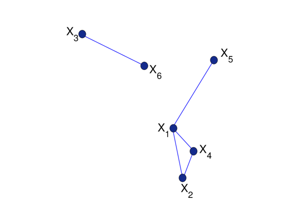
Figure 12: Graph encoding the Markov structure of the model given by precision matrix (4.3).

We sampled $300$ observations from a Multivariate Normal with mean zero and precision matrix

$$\begin{pmatrix}18.18&-6.55&0&2.26&-6.27&0\\ -6.55&14.21&0&-4.90&0&0\\ 0&0&10.47&0&0&-3.65\\ 2.26&-4.90&0&10.69&0&0\\ -6.27&0&0&0&27.26&0\\ 0&0&-3.65&0&0&7.41\end{pmatrix}$$ (4.3)

whose conditional independence structure is given by the graph in Figure 12. We fit the model described in Section 3 using a uniform prior for each $V_{i}\in{\mathbb{B}^{2}}$ and $r=0.25$. We employed hybrid random walk proposals in which we move all five vertices $\left\{V_{i}\right\}$ independently according to the diffusion-inspired random walk described in Section 3.2 with probability $0.85$; replace one uniformly selected vertex $V_{i}$ with a uniform draw from $\textsf{Un}({\mathbb{B}^{2}})$ with probability $0.05$; and replace all five vertices with independent unoform draws from $\textsf{Un}({\mathbb{B}^{2}})$ with probability $0.10$. We sampled $1\,000$ observations from the posterior after a burn in of $750\,000$. Results are summarized in Table 4

Graph Topology	Posterior Probability
$\vrule width=0.0pt,height=10.0pt,depth=0.0pt{\color[rgb]{1,0,0}\bf[1,2,4]}{\color[rgb]{1,0,0}\bf[1,5]}{\color[rgb]{1,0,0}\bf[3,6]}$	$0.152$
$[1,5][2,3,4][2,3,6]$	$0.072$
$[1,2,3,4,6][1,5]$	$0.069$
$[1,4][2,4][2,3,6]$	$0.055$
$[1,2,4][2,3,4][1,5][3,6]$	$0.052$

Table 4: The five models with highest estimated posterior probability. The true model is shown in bold.

4.2.3 Factorization Based on Nerves

While Gaussian joint distributions are determined entirely by the bivariate marginals, and so only edges appear in their complete-set factorizations (see (2.1a)); more complex dependencies are possible for other distributions. The familiar example of the joint distribution of three Bernoulli variables $X_{1}$, $X_{2}$, $X_{3}$ each with mean $1/2$, with $X_{1}$ and $X_{2}$ independent but $X_{3}=(X_{1}-X_{2})^{2}$ (so that $\left\{X_{i}\right\}$ are only pairwise independent) has only the complete set $\{1,2,3\}$ in its factorization.

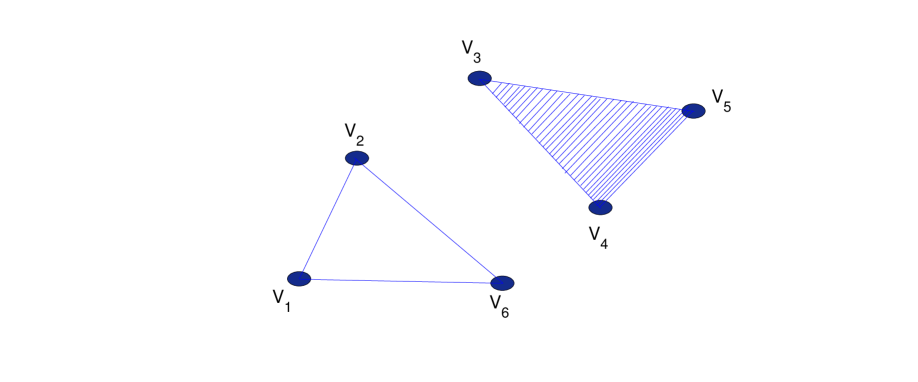
Figure 13: Graph encoding the Markov structure of the model given in (4.4).

Consider now a model with the graphical structure illustrated in Figure 13 whose density function, if it is continuous and strictly positive ((see Lauritzen, 1996, Prop. $3.1$)), admits the complete-set factorization:

$$f(x\mid{\mathcal{G}},\theta)=c_{\mathcal{G}}\,\phi(x_{1},x_{2})\phi(x_{1},x_{6})\phi(x_{2},x_{6})\cdot\phi(x_{3},x_{4},x_{5}).$$ (4.4a)

For illustration we will take each $$\phi(\cdot) \theta=4 f(x\mid{\mathcal{G}},\theta)$$ to be a Clayton copula density (see (4.1b)). For simplicity we specify the same value for each association parameter, so is given by (4.4a) with

$$\phi(x,y) =5 (x^{-4}+y^{-4}-1)^{-9/4} (x\,y)^{-5}$$ (4.4b)

$$\phi(x,y,z) =30 (x^{-4}+y^{-4}+z^{-4}-2)^{-13/4} (x\,y\,z)^{-5}.$$ (4.4c)

In earlier examples we associated graphical structures (i.e., edge sets) with $1$-skeletons of nerves. We now associate hypergraphical structures (i.e., abstract simplicial complexes that may include higher-order simplexes) with the entire nerves, with maximal simplices associated with complete-set factors. For example: the Alpha complex computed from the vertex set displayed in Table 5 with $r=0.40$ has $\{3,4,5\}\{1,2\}\{1,6\}\{2,6\}$ as its maximal simplices (Figure 14). By associating a Clayton copula to each of these hyperedges we recover the model shown in (4.4).

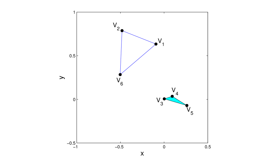
Figure 14: Alpha complex corresponding to the vertex set in Table 5 and $r=\sqrt{0.075}$.

Coordinate	$V_{1}{}$	$V_{2}{}$	$V_{3}{}$	$V_{4}{}$	$V_{5}{}$	$V_{6}{}$
$x$	$-0.0936$	$-0.4817$	$0.0019$	$0.0930$	$0.2605$	$-0.5028$
$y$	$0.6340$	$0.7876$	$0.0055$	$0.0351$	$-0.0702$	$0.2839$

Table 5: Vertex set used for generating a factorization based on nerves.

We use the same prior and proposal distributions constructed in Section 3.2 from point distributions in ${\mathbb{R}}^{d}$; what has changed is the way the nerve is being used: as a hypergraph whose maximal hyperedges represent factors. One complicating factor is the need to evaluate the normalizing factor $c_{\mathcal{G}}$ for each graph ${\mathcal{G}}$ we encounter during the simulation; unavailable in closed form, we use Monte Carlo importance sampling to evaluate $c_{\mathcal{G}}$ for each new graph, and store the result to be reused when ${\mathcal{G}}$ recurs.

We anticipate that uniform draws $V_{i}\mathrel{\mathop{\sim}\limits^{\mathrm{iid}}}\textsf{Un}({\mathbb{B}^{2}})$ will give high probability to clusters of three or more points within a ball of radius $r$, favoring higher-dimensional features (triangles and tetrahedra) in the induced hypergraph encoding the Markov structure of $\left\{X_{i}\right\}$. To explore this phenomenon, we compare results for uniform draws with those from a repulsive process under which clusters of three or more points are unlikely to lie within a ball of radius $r$, hence favoring hypergraphs with only edges.

We began by sampling $650$ observations from model (4.4) with ${\mathcal{A}}=\textrm{Alpha}$ and $r=0.40$, with independent uniform prior distributions for the vertices $V_{i}\mathrel{\mathop{\sim}\limits^{\mathrm{iid}}}\textsf{Un}({\mathbb{B}^{2}})$ on the unit ball in the plane. The Metropolis/Hastings proposals for the vertex set are given by a mixture scheme:

• A random walk for each $V_{i}$ as described in Section 3.2, with step size $\eta=0.020$. This proposal is picked with probability $0.94$

• An integer $1\leq k\leq 6$ is chosen uniformly and, given $k$, a subset of size $k$ from $\left\{1,2,3,4,5,6\right\}$ is sampled uniformly; the vertices corresponding to those indices are replaced with random independent draws from $\textsf{Un}({\mathbb{B}^{2}})$. This proposal is picked with probability $0.06$, $0.01$ for each $k$.

For $\theta$ we used the same standard exponential prior distribution and reflecting uniform random walk proposals described in Example 4.2.1.

Using $5\,000$ posterior samples after a burn-in period of $95\,000$ iterations, the models with highest posterior probability are summarized in Table 6.

Maximal Simplices	Posterior Probability
$\vrule width=0.0pt,height=10.0pt,depth=0.0pt{\color[rgb]{1,0,0}\bf\{3,4,5\}}{\color[rgb]{1,0,0}\bf\{1,2\}}{\color[rgb]{1,0,0}\bf\{2,6\}}{\color[rgb]{1,0,0}\bf\{1,6\}}$	$0.609$
$\{1,2,6\}\{3,4\}\{4,5\}\{3,5\}$	$0.161$
$\{3,5\}\{1,6\}\{3,4\}\{1,2\}\{2,6\}$	$0.137$

Table 6: Highest posterior factorizations with uniform prior for model of (4.4) and Figure 13 (true model is shown in bold).

To penalize higher-order simplexes we used a Strauss repulsive process (Strauss, 1975) conditioned to have $p$ points in ${\mathbb{B}^{d}}$ as prior distribution for the vertex set, with Lebesgue density

$$g(v)\propto\gamma^{\#\left\{(i,j):~{}{\textrm{dist}\left(v_{i},v_{j}\right)}<2R\right\}}$$

for some $0<\gamma\leq 1$, penalizing each pair of points closer than $2R$. Simulation results for this prior (with $R=0.7r$ and $\gamma=0.75$) are summarized in Table 7. The posterior mode is far more distinct for this prior than for the uniform prior shown in Table 6.

Maximal Simplices	Posterior Probability
$\vrule width=0.0pt,height=10.0pt,depth=0.0pt{\color[rgb]{1,0,0}\bf\{3,4,5\}}{\color[rgb]{1,0,0}\bf\{1,2\}}{\color[rgb]{1,0,0}\bf\{2,6\}}{\color[rgb]{1,0,0}\bf\{1,6\}}$	$0.824$
$\{1,2,6\}\{3,4,5\}$	$0.111$
$\{1,2,6\}\{3,4\}\{3,5\}\{4,5\}$	$0.002$

Table 7: Highest posterior factorizations with Strauss prior (true model is shown in bold).

In a further experiment with $\gamma=0.35$, the posterior was concentrated on factorizations without any triads.

4.2.4 ${\mathcal{G}}$ Outside the Space Generated by ${\mathcal{A}}$

In the simulation studies of Sections 4.2.1–4.2.3 the class of sets ${\mathcal{A}}$ used to compute the nerve was known. In this example we investigate the behavior of our methodology when the class of convex sets used to fit the model differs from that used to generate the true graph. We consider three possibilities: ${\mathcal{A}}=\textrm{Alpha}$ in ${\mathbb{R}}^{2}$, ${\mathcal{A}}=\textrm{Alpha}$ in ${\mathbb{R}}^{3}$ and ${\mathcal{A}}=\textrm{\v{C}ech}$ in ${\mathbb{R}}^{2}$. We performed two experiments: one when the graph is feasible for each the three classes, and another example where the graph could be generated by only two of the classes.

First consider a model with junction tree factorization:

$$f_{\theta}({\mathbf{x}})=\frac{\psi_{\theta}(x_{1},x_{3})\psi_{\theta}(x_{2},x_{3},x_{4})\psi_{\theta}(x_{5})}{\psi_{\theta}(x_{3})},$$ (4.5)

whose conditional independence structure given by the graph of Figure 15. Again, the clique marginals are specified as a Clayton copula with $\theta=4$. We simulated $300$ samples from this distribution.

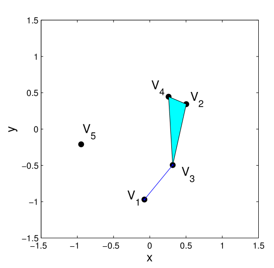
Figure 15: Graph encoding the Markov structure of the model given in (4.5).

We fitted the model with each of the three classes of convex sets using the Metropolis Hastings algorithm of Section 3.2 with random walk proposals on ${\mathbb{B}^{d}}$ (where $d=2$ or $3$, depending on ${\mathcal{A}}$). Algorithm 1 was used to enforce decomposability, using $r=0.40$ and $\eta=0.020$. The same exponential prior and uniform reflecting random-walk proposals for $\theta$ were used as in Example 4.2.1. Results of $1\,000$ samples after a burn-in period of $50\,000$ draws are summarized in Table 8. Not surprisingly, the posterior mode coincided with the true model in all three cases.

Nerve	HPP Models	Posterior
Alpha in ${\mathbb{R}}^{2}$	${\color[rgb]{1,0,0}\bf[1,3]}{\color[rgb]{1,0,0}\bf[2,3,4]}{\color[rgb]{1,0,0}\bf[5]}$	$0.964$
	$[1,3][2,3,4][1,5]$	$0.012$
	$[1,3,4][2,3,4][5]$	$0.012$
Alpha in ${\mathbb{R}}^{3}$	${\color[rgb]{1,0,0}\bf[1,3]}{\color[rgb]{1,0,0}\bf[2,3,4]}{\color[rgb]{1,0,0}\bf[5]}$	$0.982$
	$[1,3][2,3][3,4][5]$	$0.011$
	$[1][2,3,4][5]$	$0.003$
Čech in ${\mathbb{R}}^{2}$	${\color[rgb]{1,0,0}\bf[1,3]}{\color[rgb]{1,0,0}\bf[2,3,4]}{\color[rgb]{1,0,0}\bf[5]}$	$0.595$
	$[1,2,3,4][5]$	$0.179$
	$[1,2,3,4,5]$	$0.168$

Table 8: Models with highest posterior probability. The table is divided according to the class of convex sets used when fitting the model. The true model is shown in bold.

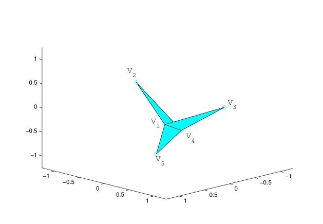
Figure 16: Graph encoding the Markov structure of the model given in (4.6).

The second model we considered has junction tree factorization:

$$f_{\theta}({\mathbf{x}})=\frac{\psi_{\theta}(x_{1},x_{2},x_{4})\psi_{\theta}(x_{1},x_{3},x_{4})\psi_{\theta}(x_{1},x_{4},x_{5})}{\left(\psi_{\theta}(x_{1},x_{4})\right)^{2}}.$$ (4.6)

The corresponding graph cannot be obtained from an Alpha complex in ${\mathbb{R}}^{2}$, but it is feasible for an Alpha complex in ${\mathbb{R}}^{3}$ (Figure 16) or a Čech complex in ${\mathbb{R}}^{2}$. Using the same Clayton clique marginals before, we sampled $300$ observations from this distribution and fitted the model using the three classes of convex sets. Results from $1\,000$ samples after a burn-in period of $75\,000$ are summarized in Table 9. Observe that for Alpha complexes in ${\mathbb{R}}^{2}$, there is no clear posterior mode (unlike the previous example, or Sections 4.2.1 and 4.2.3). The posterior mode for the Čech complex in ${\mathbb{R}}^{2}$ and the Alpha complex in ${\mathbb{R}}^{3}$ both match the true model.

Nerve	HPP Models	Posterior
Alpha in ${\mathbb{R}}^{2}$	[1,2][1,3,4][1,4,5]	0.214
	[1,2,4][1,3,4][1,3,5]	0.115
	[1,2,4][1,3,4][3,4,5]	0.112
Alpha in ${\mathbb{R}}^{3}$	[1,2,4][1,3,4][1,4,5]	0.976
	[1,2,3,4][1,4,5]	0.016
	[1,2,4][1,3][1,4,5]	0.009
Čech in ${\mathbb{R}}^{2}$	[1,2,4][1,3,4][1,4,5]	0.758
	[1,2,4][1,3,4][1,3,5]	0.177
	[1,2,4][1,3,4][4,5]	0.148

Table 9: Models with highest posterior probability, for each class of convex sets. The true model (shown in bold) is unattainable for Alpha complexes in ${\mathbb{R}}^{2}$.

4.3 Comparative performance analysis with state-of-the-art

We compared the performance of our method to Feature Inclusion Stochastic Search (FINCS), proposed by Scott and Carvalho (2008), and the adaptive LASSO as described in the paper by Fan et al. (2009). The criterium for the comparison was given by estimating the counts of specific subgraphs of a set of graphs of size $50$. This is, we generated $100$ graphs of size $50$, and we computed the absolute counts for the following subgraphs: triangles, 4-cycles, 5-cycles, 3-stars, 4-stars, and 5-stars, for the true graph and for the estimated network by our method and its competitors, then we computed the absolute difference between the counts for the true and estimated graph and then divided by the count for the true graph. We denote by an $*$ the counts of induced subgraphs; this measures the performance of the methods under decomposability. We generated the set of true networks from an Erdös-Rényi random graph model with $\alpha=0.05$, so we are in a regime that can be called sparse.

To fit our method, we assumed an uniform distribution on the unit ball in ${\mathbb{R}}^{3}$ for the vertex set and for the radius of each vertex an $\textsf{Ex}(0.1)$ as priors. For the positions of the vertices we used the same proposals as in Examples 4.2.1 - 4.2.4. For each radius we implemented a mixture of random walks reflecting at $0$ as proposal. We used the nerve corresponding to the Cech complex. We set up FINCS with a probability of $0.1$ for resampling moves and a probability of $0.1$ for global moves. For the adaptive LASSO we set up $\gamma=0.5$ and $\Omega$ was initialized as the inverse of the sampled covariance matrix. Subgraphs were counted using the igraph command graph.subisomorphic.lad. When computing the normalized error, we adopted the convention $0/0=0$. For the induced subgraphs, we only compute the error of the Bayesian procedure and Lasso over the set of non-decomposable graphs. For the simulation displayed in Table 10 all $100$ graphs were non-decomposable.

Subgraph	Bayes	FINCS	Lasso
triangles	$0.083\pm 0.07$	$0.125\pm 0.17$	$0.208\pm 0.12$
4- cycles	$0.062\pm 0.10$	$0.123\pm 0.16$	$0.166\pm 0.10$
5- cycles	$0.086\pm 0.07$	$0.112\pm 0.14$	$0.124\pm 0.08$
3- stars	$0.103\pm 0.08$	$0.139\pm 0.12$	$0.211\pm 0.08$
4- stars	$0.087\pm 0.08$	$0.096\pm 0.16$	$0.115\pm 0.11$
5- stars	$0.201\pm 0.10$	$0.183\pm 0.14$	$0.174\pm 0.06$
$\text{4- cycles}*$	$0.146\pm 0.12$	$0.930\pm 0.07$	$0.229\pm 0.12$
$\text{5- cycles}*$	$0.128\pm 0.13$	$1\pm 0$	$0.174\pm 0.08$

Table 10: Estimated normalized errors for counts of specific subgraphs for our method, FINCS and adaptive LASSO.

Results are summarized in Table 10. Our method incurred into less errors on average compared to our competitors for almost all subgraphs. The exception was the $5-$star. We also observed that FINCS outperformed the LASSO for almost all regimes, with exception of the $5-$star.

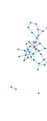
Figure 17: Here we compare the true model, which was sampled from the ERGM used in Table 11, and the fitted model, using our method (again, as in Table 11). The edges that were added by our method (with respect to the true graph) are highlighted in red. The edges that were deleted by our method are highlighted in green.

We performed another simulation, now assuming an exponential random graph model for the true graph. The simulation of the true graphs was implemented using the R package statnet. We used the formula edges+triangles+kstar(3), with coef=c(-3.2,0.95,0.005); this specification encourages the presence of triangles and 3-stars. These choices produce graphs with twice the 3-stars and 3 times more triangles than an Erdös-Rényi  with $\alpha=0.05$, while having approximately the same density. The objective of this experiment is to investigate the behavior of our method when the true graph has more structure than the typical realization of an Erdös-Rényi  model. Results are summarized in Table 11; they are similar to what was observed in the previous experiment. We observed an improvement regarding the counts of triangles, this is not surprising since geometric random graphs tend to have more triangles than realizations from an Erdös-Rényi model. In Figure 17 we compare the true model (as generated from the ERGM just described) and the fitted model for a single realization. In this regime, graphs tend to be non-decomposable. We estimated the proportion of decomposable graphs from a sample of 1,000 networks sampled from the ERGM used to obtain the simulation in Table 11, and obtained 0.302 as the result. For the simulation displayed in Table 11, $72$ out of the $100$ graphs were non-decomposable.

Subgraph	Bayes	FINCS	Lasso
triangles	$0.071\pm 0.04$	$0.134\pm 0.14$	$0.217\pm 0.09$
4- cycles	$0.067\pm 0.06$	$0.121\pm 0.12$	$0.154\pm 0.04$
5- cycles	$0.075\pm 0.09$	$0.118\pm 0.11$	$0.131\pm 0.13$
3- stars	$0.092\pm 0.07$	$0.144\pm 0.14$	$0.236\pm 0.12$
4- stars	$0.086\pm 0.09$	$0.115\pm 0.15$	$0.117\pm 0.10$
5- stars	$0.214\pm 0.09$	$0.122\pm 0.13$	$0.121\pm 0.06$
$\text{4- cycles}*$	$0.152\pm 0.12$	$0.720\pm 0.07$	$0.214\pm 0.10$
$\text{5- cycles}*$	$0.133\pm 0.10$	$0.720\pm 0.13$	$0.163\pm 0.08$

Table 11: Estimated normalized errors for counts of specific subgraphs for our method, FINCS and adaptive LASSO. The true graphs were sampled from an ERGM that encouraged the presence of triangles and 3-stars.

4.3.1 Scalability

Here we discuss scalability of the proposed method and of the competing methods ( Fan et al. (2009), Scott and Carvalho (2008)) to better appreciate the cost incurred in producing the errors in Tables 10 and 11. Since the implementation of the proposed and competing methods available to us are in different programming languages, which influence greatly the actual runtime, we outline such a discussion in theory, in terms of key quantities that influence scalability, including number of nodes $n$, number of edges $m$, and number of cliques $k$. We also distinguish two tasks: the task of estimating the parameter of a model-based representation of a (hyper)graph, and the task of generating $b$ (hyper)graphs from an estimated model-based representation.

Regarding the task of estimating parameters from an observed (hyper)graph, the proposed methods requires estimating parameters $\left\{V\right\},r$, and the estimation complexity scales as $O(S(n)+k^{3})$, where $S(n)$ denotes the complexity of matrix multiplication. The method by Scott and Carvalho (2008) requires estimating parameters ${\mathcal{G}}$, and the estimation complexity scales as $O(S(n)+k)$. The lasso requires estimating parameters $\Sigma^{-1}$, and the estimation complexity scales as $O(n^{3})$.

Regarding the task of generating $b$ (hyper)graphs from an estimated model-based representation, the proposed methods scales as $O(bn^{2})$. This is because the complexity of computing the 2-skeleton of the Cech complex scales as $O(n^{2})$. Alternative representations lead to different scaling: computing the Delaunay triangulation scales as $O(n\log n)$, and computing the the Alpha complex scales as $O(n^{2})$. The method by Scott and Carvalho (2008) scales as $O(bnm)$, where typically $m$ is much larger than $n$. For the lasso, this statement does not apply.

To illustrate how our method scales up with respect to the number of variables, we ran the experiment summarized in Table 12. We obtained the graphs from the nerves of Čech complexes and employed the method proposed by (Atay-Kayis and Massam, 2005) to compute the normalizing constants of non-decomposable graphs. The MCMC was performed on a 2.5GHz desk computer with 4GB of RAM. Our method was implemented using Matlab (MathWorks).

N Variables	Burn-in	N Iterations	Time
$\vrule width=0.0pt,height=10.0pt,depth=0.0pt\par 4$	$50,000$	$10,000$	$7m$
$40$	$50,000$	$10,000$	$2h~{}11m$
$400$	$50,000$	$10,000$	$3d~{}2h~{}17m$

Table 12: This experiment illustrates how our method scales up with respect to the number of variables.

4.4 Real data analysis

4.4.1 Fisher’s Iris data

We applied our method to Fisher’s Iris data set. Variables include: sepal length (1), sepal width (2), petal length (3), and petal width (4). The objective is to find the conditional independence structure given a family of distributions for the likelihood (e.g. Gaussian, Clayton copula). A summary of the distribution of this data set is given in Table 13

Variable	SL	SW	PL	PW
Sepal length	$0.4043$
Sepal width	$0.0938$	$0.1040$
Petal length	$0.3033$	$0.0714$	$0.3046$
Petal width	$0.0491$	$0.0476$	$0.0488$	$0.0754$

Table 13: Estimated variances and covariances for the Iris data.

We first describe the specification we used for the random geometric graph, then we will make our choices for the Hyper-Markov law and the likelihood explicit. For the RGG we assumed an uniform distribution of the vertices on the unit ball in ${\mathbb{R}}^{3}$ and for the radius of each vertex an $\textsf{Ex}(0.1)$, distribution was assumed. For the positions of the vertices we used the same proposals as in Examples 4.2.1 - 4.2.4. For each radius we used a mixture of random walks reflecting at $0$ as proposal. For the likelihood function and Hyper-Markov law we used the following specifications: A multivariate normal distribution for the likelihood with an HIW as Hyper-Markov law.

For our choice for the likelihood and Hyper-Markov law, we adopted the same values for the hyperparameters as (Roverato, 2002) did, this is, the prior for the precision matrix centered at $I$ and $\delta=3$. We used the method proposed by (Atay-Kayis and Massam, 2005) to deal with the normalizing constants of non-decomposable graphs. We ran the MCMC with $300\,000$ iterations as burn-in and kept the last $10\,000$ for analysis.

Results for the first choice are summarized in Table 14. Here we display the $9$ models with highest posterior probability. All the posterior probability was concentrated in this models. Our posterior mode coincides with the one reported by (Roverato, 2002), but we obtained different results for the rest of the models. We attribute this difference to the fact that we used different priors for graph space; ours being non-uniform.

Maximal Simplices	Posterior Probability
$\vrule width=0.0pt,height=10.0pt,depth=0.0pt\{1,2\}\{1,3\}\{2,4\}\{3,4\}$	$0.3465$
$\{2\}\{1,3\}\{3,4\}$	$0.2835$
$\{1,3\}\{2,3\}\{4\}$	$0.1999$
$\{1,2\}\{1,3\}\{4\}$	$0.1540$
$\{1,2\}\{1,4\}\{2\}$	$0.0116$
$\{1,4\}\{2\}\{3,4\}$	$0.0026$
$\{1,2\}\{1,3\}\{3,4\}$	$0.0016$
$\{1,3\}\{2,3\}\{3,4\}$	$0.0002$
$\{1,4\}\{1,3\}\{2,3\}\{3,4\}$	$0.0001$

Table 14: Highest posterior factorizations with uniform prior and Gaussian distribution for Fisher’s Iris data set.

Maximal Simplices	Frequency as posterior mode
$\vrule width=0.0pt,height=10.0pt,depth=0.0pt\{1,2\}\{1,3\}\{2,4\}\{3,4\}$	$0.68$
$\{1,3\}\{2,3\}\{4\}$	$0.16$
$\{1,2\}\{2,3\}\{2,4\}$	$0.08$
$\{1,4\}\{2,4\}\{3,4\}$	$0.04$
$\{1,4\}\{1,3\}\{2\}$	$0.04$

Table 15: Results from missing data simulation: We fit our model the same way as in Table 14, but leaving one row out each time and imputing it as missing data. In this table we report the frequency by which each factorization appeared as posterior mode.

We conducted another simulation, where we assessed the robustness of the inference for the Gaussian graphical model via tools from missing data. We fit our model deleting one row of the data at a time (this is, we fit our model 50 times over incomplete data sets) and imputed the missing data using the conditional distribution of the observed data. Results are summarized in 15. For each of this simulations we computed the average distance between the predicted vector and the observed one. For FINCS, the average distance between the predicted and observed vectors (across the 50 simulations) was $3.69\pm 1.28$, while for our method it was $3.22\pm 1.15$. This is not surprising, since, in contrast to FINCS, we consider non-decomposable models.

4.4.2 Daily exchange rates data

Following Hernandez-Lobato et al. (2013), we considered daily exchange rates of eight currencies (Swiss franc, Australian dollar, Canadian dollar, Norwegian krone, Swedish krona, Euro, New Zealand dollar and British pound) with respect to the U.S. dollar. The data set consists of 717 observations, from 1 Dec., 2011, to 29 Aug., 2014. Clearly these observations are not iid, but we will not take this into account in the modeling. What makes this application interesting is the presence of a non-trivial missing data pattern. The data was downloaded from yahoo.finance.com via the R library tseries.

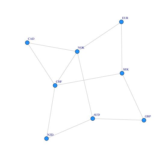
Figure 18: Posterior mode of our method when applied to daily exchange rates (with respect to US Dollar) from 1 Dec., 2011 to 29 Aug., 2014. Here CHF denotes the Swiss franc, AUD, the Australian dollar, CAD, the Canadian dollar, NOK, the Norwegian krone, SEK, the Swedish krona, EUR, the Euro, NZD, the New Zealand dollar, and GBP, the British pound.

We applied our method to these data. We assumed a uniform distribution for the vertices in the unit ball in ${\mathbb{R}}^{3}$, and that the nerve was computed from the intersection pattern of balls of different sizes. We assumed a HIW as the hyper-Markov law and a multivariate normal as the likelihood. We kept the simulated values from 5,000 iterations after 25,000 iterations of burn-in. Missing data were assumed missing at random and imputed from the model. The posterior mode is illustrated in Figure 18; it has 0.87 posterior probability. This model is non-decomposable.

5 Discussion

In this article we present a new parametrization of graphs by associating them with finite sets of points in ${\mathbb{R}}^{d}$. This perspective supports the design of informative prior distributions on graphs using familiar probability distributions of point sets in ${\mathbb{R}}^{d}$. It also induces new and useful Metropolis/Hastings proposal distributions in graph space that include both local and global moves. As suggested by Helly’s Theorem (Edelsbrunner and Harer, 2009) characterizing the sparsity of intersections of convex sets in ${\mathbb{R}}^{d}$, this methodology is particularly well suited for sparse graphs. The simple strategies presented here generalize easily to more detailed and subtle models for both priors and M/H proposals.

Our construction leads to MCMC that naturally instantiate local and global moves in graph (and hypergraph) space. The proposals that produce small perturbations on the vertex set will produce local moves with high probability, while proposals that consist in resampling a subset of the vertex set will produce, with high probability, a global move (See Figure 5).

An interesting feature of our approach is that the distribution on the space of graphs is modeled directly before the application of any specific hyper Markov law, in contrast to standard approaches in which it is the hyper Markov law that is used to encourage sparsity or other features on the graph. We think that working with the space of graphs explicitly opens a lot of possibilities for prior specification in graphical models, therefore, it is a perspective worth further study.

While coupling the focus on the first two moments and a graph representation of pairwise dependencies among variables are not restrictive modeling choices in the Gaussian graphical model framework, they become restrictive when working with graphical models in general. However, likely because of convenience, these assumptions are seldom challenged in the graphical models literature. Here we develop a geometric construction where dependence relations of higher orders can be conveniently encoded within a hypergraph. For a state of the art treatment of parametrizations of decomposable graphs, see (Cron and West, 2012).

Connected to the point above, while decomposability plays an important role in graphical models in general, it does not play any role in our construction. This is because decomposability is relevant for computations at the Hyper-Markov law level, while our construction and results are at the level of the prior on graph space.

About the space of graph where our construction puts positive mass. At this point we have two results and a conjecture for characterizing the space of feasible graphs (hypergraphs) when we consider the nerve of a set of balls in ${\mathbb{R}}^{3}$ with different radii (This is the case that should have the largest support for the distribution of graphs.)

Theorems: (i) Any graph can be embedded in $\mathbb{R}^{3}$. This is a well known result. One method that computes such embedding is the Book Algorithm, proposed by (Kainen, 1974) and (Ollmann, 1973). (ii) Any graph can be linearly embedded in $\mathbb{R}^{3}$. By ‘linearly embedded’ it is meant that the segments joining the vertices are straight lines. This is a particular case of a more general result, that every k-dimensional simplicial complex can be geometrically realized in $2k+1$ dimensions. In this case case, $k=1$. See Section 3.1 of (Edelsbrunner and Harer, 2008).

Conjecture: (iii) Such a linear embedding can be achieved using a random geometric graphs construction using balls with different radii.

Interesting questions and extensions of this idea include: (1) achieving a deeper and more detailed understanding of the subspace of graphs spanned by different specific filtrations; (2) designing priors to control the distributions of specific features of graphs such as clique size or tree width; (3) modeling directed acyclic graphs (DAGs), and (4) concrete implementation of novel Markov structures based on nerves.

This methodology generates only graphs that are feasible for the particular filtration chosen. Although we do have some insight about which graphs can and cannot be generated by a specific filtrations, a more complete and formal understanding of this aspect of the problem would be useful.

We used very simple prior distributions for the purpose of illustrating the core idea of the methodology. It is natural in this approach to incorporate tools from point processes into graphical models to define new classes of priors for graph space. Future developments in our research will involve a range of repulsive and cluster processes.

The parametrization we propose can be used to represent Markov structures on DAGs, but the strategies for obtaining such graphs from nerves will be different and will establish stronger connections between Graphical Models and computational topology.

The present work is related to that of Pistone et al. (2009) in which a nerve of convex subsets in ${\mathbb{R}}^{d}$ is used to obtain Markov structures for a distribution, an extension of the abstract tube theory of Naiman and Wynn (1997). This new perspective allows for constructions that generalize the idea of junction trees. By modifying our methodology according to this framework (personal communication from H. Wynn suggests that this is feasible) we hope to fit models that factorize according to those novel Markov structures.

Another possible extension of this work is to discretize the set from which the vertex set is sampled (e.g., use a grid). Such discretization may improve the behaviour of the MCMC; it would also allow the use of a nonparametric form for the prior on the vertex set, leading to more flexible priors on graph space.

While we illustrated the new construction for Bayesian inference, in a situation where we observe high-dimensional vectors and we want to infer the dependencies among their components, the proposed construction can be easily used to build a likelihood in situations where we have direct observations about the facets of hypergraph. Such observations occur naturally in applications; just think of how one would encode the structure among individuals revealed by pictures on Facebook. Each picture has one or more people. A picture with three people is naturally encoded as a 3-facet, rather than as 3 individual edges, as currently done, arguably for lack of likelihood models for hyper graphs.

References

Appendix A Filtrations and Decomposability in Random Geometric Graphs

A filtration is a sequence of simplicial complexes that properly include their predecessors:

Definition A.1 (Filtration).

A filtration for a simplicial complex ${\mathcal{K}}$ is a sequence ${\mathscr{L}}=\left\{{\mathcal{K}}^{0},{\mathcal{K}}^{1},\ldots,{\mathcal{K}}^{k}\right\}$ of simplicial complexes such that

$$\varnothing={\mathcal{K}}^{0}\subset{\mathcal{K}}^{1}\subset\ldots\subset{\mathcal{K}}^{k}={\mathcal{K}},$$

with all inclusions proper.

Filtrations are commonly used in computational geometry and topology to construct efficient algorithms for computing specific nerves including the Alpha complex [Edelsbrunner and Mücke, 1994]. The simplicial complexes constructed in Section 2.2 from families of convex sets lead to filtrations as the convex sets are enlarged, by increasing the radius parameter $r$.

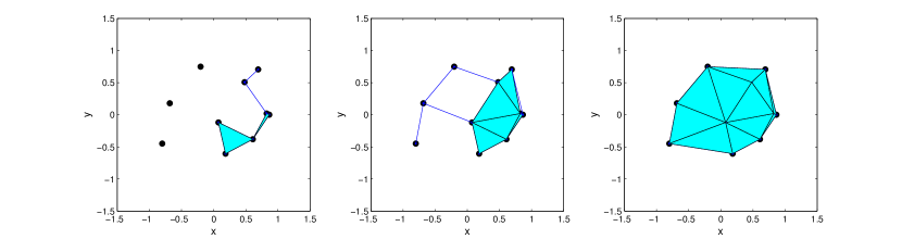
Figure 19: Filtration of Alpha complexes, (a) $r=\sqrt{0.10}$, (b) $r=\sqrt{0.20}$ and (c) $r=\sqrt{0.75}$.

Although much of the graphical models literature focuses on Markov structures derived from decomposable graphs, those constructed in Section 2.2 from $1$-skeletons of Čech and Alpha complexes need not be decomposable (see Figure 19). In Algorithm 1 we present an adaptation of this construction that generates decomposable graphs, for use in applications that require them. In Sections 3 and 4 we present methodology and examples for both decomposable and unrestricted model spaces.

The central idea for generating decomposable graphs from filtrations is to note that the complex ${\mathcal{A}}({\mathcal{V}},0)$ for $r=0$ is disconnected and hence decomposable; as the radius $r$ increases, if one adds edges only if the resulting graph is decomposable, then decomposability will hold for all $r\geq 0$. This procedure is formalized in Algorithm 1.

input : a filtration ${\mathscr{L}}=\left\{{\mathcal{K}}^{0},{\mathcal{K}}^{1},\ldots,{\mathcal{K}}^{k}\right\}$

return : a weakly decomposable graph ${\mathcal{G}}$

$m=0$; $i=0$; ${\mathcal{G}}_{0}=\varnothing$;

while $i<k\mathbf{~{}and~{}}{\mathcal{K}}^{i+1}\neq\varnothing$ do

       $\tau_{i}=\left\{\kappa\in{\mathcal{K}}^{i+1}\setminus{\mathcal{K}}^{i}\mbox{ such that }|\kappa|=2\right\}$; // the edges in the set difference and denote $\tau_{i,s}$ as the $s$th edge

       if $\tau_{i}\neq\varnothing$ then

             $P=|\tau_{i}|$;

             for $s=1$ to $P$ do

                   ${\mathcal{G}}^{\prime}={\mathcal{G}}_{m}\bigcup\tau_{i,s}$ ; // propose adding the edge

                   if $\sharp({\mathcal{G}}^{\prime})<\sharp({\mathcal{G}}_{m})$ // fewer connected components?

                   then

                         ${\mathcal{G}}_{m+1}={\mathcal{G}}^{\prime}$ ; // accept the proposal

                         $m=m+1$;

                  else

                         $[c_{i}]={\mathscr{C}}({\mathcal{G}}_{m})$ ; // the cliques

                         $[s_{i}]={\mathscr{S}}({\mathcal{G}}_{m})$ ; // the separators

                         $[v_{1},v_{2}]=\tau_{i,s}\quad$; // the proposed edge

                         if  $\exists i\neq j,k$ with $v_{1}\in c_{i},v_{2}\in c_{j}$ and $c_{i}\bigcap c_{j}=s_{k}$  then

                               ${\mathcal{G}}_{m+1}={\mathcal{G}}^{\prime}$ ; // accept the proposal

                               $m=m+1$;

                              

                        

                  

            

      $i=i+1$;

      

${\mathcal{G}}={\mathcal{G}}_{m}$

Algorithm 1 The algorithm takes as input a filtration of $k$ abstract complexes and returns a decomposable graph that is a subset of the $1$-skeleton of the $k$-th complex.

Proposition A.1.

The graph ${\mathcal{G}}$ produced by Algorithm 1 is decomposable.

Proof.

The algorithm is initialized with the decomposable empty graph, and decomposability is tested with each proposed addition of an edge (i.e., a $1$-simplex in ${\mathscr{L}}$). The decomposability test is taken from [Giudici and Green, 1999, Theorem $2$]. Since only finitely many edges may possibly be added, ${\mathcal{G}}$ is decomposable by construction. ∎

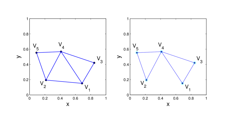
Figure 20: (a) Proximity graph computed from the vertex set given in Table 16. (b) The decomposable graph computed from the same vertex set using Algorithm 1. The edge $(1,2)$ is not included in the decomposable graph.

A.1 Example

We first illustrate the algorithm on a simple example, based on the five points in ${\mathbb{R}}^{2}$ shown in Figure 20 and given in Table 16. The graph induced by a Čech complex with $r=0.5$ will not be decomposable. Table 17 presents the evolution of cliques and separators with increasing $r$, as edges are proposed for inclusion in Algorithm 1. The first three proposed edge additions are accepted, but the proposal to add edge $(1,2)$ at radius $r=0.474$ is rejected, since the intersection of prime components $\{1,3\}$ and $\{2,4,5\}$ is empty, and therefore not a separator.

Coordinate	$V_{1}$	$V_{2}$	$V_{3}$	$V_{4}$	$V_{5}$
$\vrule width=0.0pt,height=10.0pt,depth=0.0ptx$	$0.686$	$0.214$	$0.846$	$0.411$	$0.089$
$y$	$0.151$	$0.194$	$0.420$	$0.567$	$0.553$

Table 16: Vertex set used to illustrate Algorithm 1.

Cliques	Separators	r	Update
$[1][2][3][4][5]$	$-$	0	$-{}$
$[1,3][2][4][5]$	$-$	0.313	$\left(1,3\right)$
$[1,3][2][4,5]$	$-$	0.321	$\left(4,5\right)$
$[1,3][2,5][4,5]$	$[5]$	0.379	$\left(2,5\right)$
$[1,3][2,4,5]$	$-$	0.421	$\left(2,4\right)$
$[1,3][3,4][2,4,5]$	$[3][4]$	0.459	$\left(3,4\right)$
$[1,3][3,4][2,4,5]$	$[3][4]$	0.474	$\sim\left(1,2\right)$
$[1,3,4][2,4,5]$	$[4]$	0.498	$\left(1,4\right)$

Table 17: Evolution of cliques and separators in the junction tree representation of ${\mathcal{G}}$ as edges are added according to Algorithm 1. The proposed addition of edge $\left(1,2\right)$ is rejected.

A.2 Algorithm deletes few edges

It is interesting to note that the number of proposed edge additions that are rejected by the algorithm is typically quite small. To illustrate this we applied Algorithm 1 to a filtration of Čech complexes corresponding to $100$ points sampled uniformly from the unit square, with radius $r=0.05$. In Figure 21 the graph ${\mathcal{G}}$ output by the algorithm is compared to the $1$-skeleton of the Čech complex (with no decomposability restriction) with the same radius $r=0.05$. Few edges appear in the Čech complex but not in ${\mathcal{G}}$. This occurs because geometric graphs tend to be triangulated, in the sense that if edges $\left(v_{1},v_{2}\right)$ and $\left(v_{2},v_{3}\right)$ belong to a geometric graph, then very likely the edge $\left(v_{1},v_{3}\right)$ will also be in the graph, preserving decomposability.

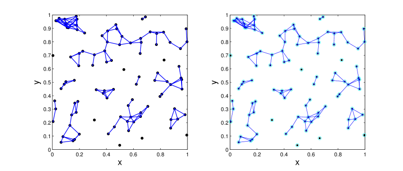
Figure 21: (a) The $1$-Skeleton of Čech complex given the displayed point set and $r=0.05$. (b) The decomposable graph for the same complex, point set, and radius output by Algorithm 1.

References

- Atay-Kayis and Massam [2005] Aliye Atay-Kayis and Hélène Massam. A Monte Carlo method to compute the marginal likelihood in non decomposable graphical Gaussian models. 92(2):317–335, 2005.
- Besag [1974] Julian E. Besag. Spatial interaction and the statistical analysis of lattice systems (with discussion). 36(2):192–236, 1974.
- Besag [1975] Julian E. Besag. Statistical analysis of non-lattice data. 24(3):179–195, 1975.
- Brooks et al. [2003] Stephen P. Brooks, Paolo Giudici, and Gareth O. Roberts. Efficient construction of reversible jump markov chain Monte Carlo proposal distributions. 65(1):3–55, 2003.
- Carvalho et al. [2007] Carlos M. Carvalho, Hélène Massam, and Mike West. Simulation of hyper-inverse Wishart distributions in graphical models. 94(3):719–733, 2007.
- Clayton [1978] David G. Clayton. A model for association in bivariate life tables and its applications in epidemiological studies of familial tendency in chronic disease incidence. 65(1):141–151, 1978.
- Cron and West [2012] Andrew Cron and Mike West. Models of random sparse eigenmatrices matrices with application to bayesian factor analysis. Available on-line at ftp://stat.duke.edu/pub/WorkingPapers/12-01.pdf, 2012.
- Dawid and Lauritzen [1993] A. Phillip Dawid and Steffen L. Lauritzen. Hyper Markov laws in the statistical analysis of decomposable graphical models. 21(3):1272–1317, 1993.
- Edelsbrunner and Harer [2008] Herbert Edelsbrunner and John Harer. Persistent homology— a survey. In Jacob E. Goodman, Janos Pach, and Richard Pollack, editors, Surveys on Discrete and Computational Geometry: Twenty Years Later, volume 453 of Contemporary Mathematics, pages 257–282. American Mathematical Society, 2008.
- Edelsbrunner and Harer [2009] Herbert Edelsbrunner and John Harer. Lecture notes from the course ‘Computational Topology’. Available on-line at http://www.cs.duke.edu/courses/fall06/cps296.1/, 2009.
- Edelsbrunner and Mücke [1994] Herbert Edelsbrunner and Ernst P. Mücke. Three-dimensional alpha shapes. ACM Transactions on Graphics, 13:43–72, 1994.
- Fan et al. [2009] J. Fan, Y. Feng, and Y. Wu. Network exploration via the adaptive lasso and scad penalties. The Annals of Applied Statistics, 3(2):521–541, 2009.
- Giudici and Green [1999] Paolo Giudici and Peter J. Green. Decomposable graphical Gaussian model determination. 86(4):785–801, 1999.
- Green [1995] Peter J. Green. Reversible jump Markov chain Monte Carlo computation and Bayesian model determination. 82(4):711–732, December 1995.
- Hammersley and Clifford [1971] John M. Hammersley and Peter Clifford. Markov fields on finite graphs and lattices. Unpublished, 1971.
- Hastings [1970] W. Keith Hastings. Monte Carlo sampling methods using Markov chains and their applications. 57(1):97–109, 1970.
- Heckerman et al. [1995] David Heckerman, Dan Geiger, and David M. Chickering. Learning Bayesian networks: The combination of knowledge and statistical data. 20(3):197–243, 1995.
- Hernandez-Lobato et al. [2013] J.M. Hernandez-Lobato, J.R. Lloyd, and D. Hernandez-Lobato. Gaussian process conditional copulas with applications to financial time series. In NIPS, 2013.
- Hoff [2007] Peter D. Hoff. Extending the rank likelihood for semiparametric copula estimation. 1(1):265–283, 2007.
- Huber and Wolpert [2009] Mark L. Huber and Robert L. Wolpert. Likelihood-based inference for Matérn type III repulsive point processes. 41(4):In press, 2009. Preprint available on-line at http://www.stat.duke.edu/ftp/pub/WorkingPapers/08-27.html.
- Jones et al. [2005] Beatrix Jones, Carlos Carvalho, Adrian Dobra, Christopher Hans, Christopher K. Carter, and Mike West. Experiments in stochastic computation for high-dimensional graphical models. 20(4):388–400, 2005.
- Kainen [1974] P. C. Kainen. Some recent results in topological graph theory. In Graphs and combinatorics, volume 406 of Lectore Notes in Mathematics, pages 76–108. Springer, 1974.
- Kalhe [2014] Matthew Kalhe. Topology of random simplicial complexes: a survey. AMS Contemp. Math., (620):201–222, 2014.
- Lauritzen [1996] Steffen L. Lauritzen. Graphical Models, volume 17 of Oxford Statistical Science Series. 1996.
- Mansinghka et al. [2006] Vikash K. Mansinghka, Charles Kemp, Joshua B. Tenenbaum, and Thomas L. Griffiths. Structured priors for structure learning. In Leopoldo Bertossi, Anthony Hunter, and Torsten Schaub, editors, Uncertainty in Artificial Intelligence: Proceedings of the Twenty-second Annual Conference (UAI 2006), 2006.
- Mukherjee and Speed [2008] Sach Mukherjee and Terence P. Speed. Network inference using informative priors. 105(38):14313–14318, 2008.
- Naiman and Wynn [1997] Daniel Q. Naiman and Henry P. Wynn. Abstract tubes, improved inclusion exclusion identities and inequalities and importance sampling. 25(5):1954–1983, 1997.
- Nelsen [1999] Roger B. Nelsen. An Introduction to Copulas. 1999.
- Ollmann [1973] Taylor L. Ollmann. On the book thicknesses of various graphs. In Frederick Hoffman, Roy B. Levow, and Robert S. D. Thomas, editors, Proc. 4th Southeastern Conference on Combinatorics, Graph Theory and Computing, Congressus Numerantium VIII, page 459, 1973.
- Penrose [2003] Mathew D. Penrose. Random Geometric Graphs. 2003.
- Penrose and Yukich [2001] Mathew D. Penrose and Joseph E. Yukich. Central limit theorems for some graphs in computational geometry. 11(4):1005–1041, 2001.
- Pistone et al. [2009] Giovanni Pistone, Henry Wynn, G. Sáenz de Cabezón, and Jim Q. Smith. Junction tubes and improved factorisations for Bayes nets. (unpublished), 2009.
- Robert [2001] Christian P. Robert. The Bayesian Choice: From Decision-Theoretic Foundations to Computational Implementation. Second edition, 2001.
- Robert and Casella [2004] Christian P. Robert and George Casella. Monte Carlo Statistical Methods. Second edition, 2004.
- Roverato [2002] Alberto Roverato. Hyper inverse Wishart distribution for non-decomposable graphs and its application to Bayesian inference for Gaussian graphical models. 29(3):341–411, 2002.
- Scott and Carvalho [2008] James G. Scott and Carlos M. Carvalho. Feature-inclusion stochastic search for Gaussian graphical models. 17(4):790–808, 2008.
- Sisson [2005] Scott A. Sisson. Transdimensional Markov chains: A decade of progress and future perspectives. 100(471):1077–1089, September 2005.
- Strauss [1975] David J. Strauss. A model for clustering. 62(2):467–476, 1975.
- Wong et al. [2003] Kevin K. F. Wong, Christopher K. Carter, and Robert Kohn. Hyper inverse Wishart distribution for non-decomposable graphs and its application to Bayesian inference for Gaussian graphical models. 90(4):809–830, 2003.