Three-dimensional topological phases in a layered honeycomb spin-orbital model

Abstract

We present an exactly solvable spin-orbital model based on the Gamma-matrix generalization of a Kitaev-type Hamiltonian. In the presence of small magnetic fields, the model exhibits a critical phase with a spectrum characterized by topologically protected Fermi points. Upon increasing the magnetic field, Fermi points carrying opposite topological charges move toward each other and annihilate at a critical field, signaling a phase transition into a gapped phase with trivial topology in three dimensions. On the other hand, by subjecting the system to a staggered magnetic field, an effective time-reversal symmetry essential to the existence of three-dimensional topological insulators is restored in the auxiliary free fermion problem. The nontrivial topology of the gapped ground state is characterized by an integer winding number and manifests itself through the appearance of gapless Majorana fermions confined to the two-dimensional surface of a finite system.

I Introduction

Topological phases of matter are one of the most remarkable discoveries in modern condensed-matter physics. tknn ; avron83 ; kohmoto85 ; wen90 ; volovik Instead of a local order parameter describing broken symmetries of the system, this novel state of matter is characterized by a topological invariant which is insensitive to small adiabatic deformations of the Hamiltonian. A classic example is the integer quantum Hall (IQH) effect, where the quantized Hall conductance corresponds to a topological invariant called the first Chern number or the TKNN integer. tknn Another distinctive property of IQH states is the appearance of zero-energy modes at the sample edge, despite the fact that all bulk excitations are fully gapped. Due to their topological nature, these conducting edge modes persist even in the presence of disorders. Recently, theoretical investigations have shown that similar topological insulators can be generalized to time-reversal invariant systems (quantum spin-Hall effect) kane05 ; bernevig06 ; moore07 ; roy09a and to three dimensions. fu07a ; fu07b ; roy09b Signatures of topological insulators such as quantized conductance and protected surface Dirac cone have been reported experimentally in semiconducting alloys and quantum wells. konig07 ; hsieh08 ; xia09 ; roushan09 ; chen09 Following these developments, systematic classifications of topological insulators have also been proposed. schnyder08 ; kitaev09 ; qi08

Although most discussions of topological insulators are in the context of tight-binding fermionic models or mean-field superconductors, it has been shown that topological insulators can also emerge from strongly correlated electronic systems. jackeli09 ; shitade09 ; raghu08 ; sun09 ; zhang09 An exactly solvable example is Kitaev’s anisotropic spin-1/2 model on the two-dimensional honeycomb lattice. kitaev06 As shown in his seminal paper, the spin model can be reduced to a problem of free Majorana fermions coupled to a static $Z_{2}$ gauge field. The ground state of the Kitaev model has two distinct phases. The gapped Abelian phase is equivalent to the toric code model kitaev03 whose excitations are Abelian anyons. Relevant to our discussion is the non-Abelian B phase in the presence of a magnetic field. This phase is characterized by an integer winding number $\nu=\pm 1$. Similar to IQH insulators, the non-Abelian phase also supports gapless chiral edge modes (whose chirality depends on the sign of magnetic fields) except that the edge modes here are real Majorana fermions, as contrasted to complex fermions in the case of IQH states.

There has been much effort to generalize Kitaev model to other trivalent lattices yang07 ; yao07 and to three-dimensions. si07 ; si08 ; mandal09 Probably the most notable example is the discovery of a chiral spin liquid as the ground state of Kitaev model on a decorated-honeycomb lattice. yao07 On the other hand, despite being exactly solvable, we find that most gapped phases of 3D Kitaev model is topologically trivial. chern09 The fact that the model can only be defined on lattices with coordination number 3 significantly constrains the possible Majorana hopping Hamiltonian. Recently, noting that the exact solvability of Kitaev model relies on the fact that the three spin-1/2 Pauli matrices realize the simplest (dimension-2) Clifford algebra, the so-called $\Gamma$-matrix generalization of the Kitaev model offers richer possibilities of engineering exactly solvable models with unusual phases in both 2D and 3D. levin03 ; hamma05 ; yao09 ; wu09 ; ryu09 ; nussinov09 Physically, models based on, e.g. dimension-4 $\Gamma$ matrices can be interpreted as spin-$\frac{3}{2}$ models, spin-$\frac{1}{2}\frac{1}{2}$ models, or spin-orbital models.

Based on the above $\Gamma$-matrix generalization of Kitaev model, emergent topological insulators have been demonstrated on a 3D diamond lattice with coordination number 4. wu09 ; ryu09 To construct a Kitaev-type model on such a lattice, one needs four mutually anticommuting operators for the four nearest-neighbor links. This can be easily realized using the dimension-4 $\Gamma$-matrix representation of the Clifford algebra. By exploiting the redundancy of representing two such sets of bosonic operators in terms of 6 Majorana fermions, the diamond-lattice model enjoys an effective time-reversal symmetry (TRS) which is essential to the existence of topological insulators in 3D. schnyder08 With only nearest-neighbor interactions, the diamond-lattice model reduces to a problem of two identical copies of free Majorana fermions sharing the same $Z_{2}$ gauge field. The permutation symmetry between the two fermion species thus manifests as a TRS. In the weak-pairing regime of the model, hybridization of the two Majorana species results in a gapped ground state with nontrivial topology.

A natural question to ask is whether it is possible to realize the required TRS in a Kitaev-type model via generic physical mechanisms. In this paper, we provide such an example through a natural generalization of the honeycomb Kitaev model. Using a similar $\Gamma$-matrix formalism, we study a Kugel-Khomskii-type kk spin-orbital Hamiltonian on a layered honeycomb lattice whose coordination number is 5. We further consider perturbations due to a weak magnetic field and single-ion spin-orbit interaction. In the weak-pairing regime of our model, the ground state remains gapless up to a critical field strength. The Fermi points of this critical phase are characterized by a nonzero topological invariant, hence are stable against weak perturbations. As the field strength is increased, Fermi points with opposite winding numbers eventually annihilate with each other and the spectrum acquires a gap above a critical field. Since the TRS is explicitly broken in the presence of a uniform magnetic field, the gapped phase represents a multilayer generalization of the 2D Kitaev model, and is topologically trivial in three dimensions.

On the other hand, when the sign of magnetic field alternates between successive honeycomb planes, an effective TRS is restored in the auxiliary fermionic model, and the corresponding ground state in the weak-pairing phase is equivalent to a topological superconductor belonging to symmetry class DIII in Altland-Zirnbauer’s classification. az We also show that the quantum ground state is characterized by an integer winding number, consistent with the general classification of 3D topological insulators.schnyder08 A physical consequence of the nontrivial ground-state topology is the appearance of surface Majorana fermions which remain gapless against perturbations respecting the discrete symmetries of the Hamiltonian. The specific multilayer geometry of our model also allows us to analytically demonstrate the existence of surface Majorana fermions obeying a Dirac-like Hamiltonian by relating the surface modes to the chiral edge modes of 2D Kitaev model.

II The spin-orbital model

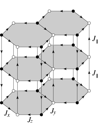
Figure 1: A layered honeycomb lattice. The five distinct nearest-neighbor links are indicated by the corresponding exchange constant. The open and filled circles denote sites belonging to the two inequivalent sites of a unit cell. The primitive vectors of the underlying Bravais lattice are $\mathbf{a}_{1}=(1,0,0)$, $\mathbf{a}_{2}=(\frac{1}{2},\frac{\sqrt{3}}{2},0)$, and $\mathbf{a}_{3}=(0,0,1)$. An arrow from site $j$ to site $k$ means the corresponding link variable $u_{jk}=+1$.

We study a Kugel-Khomskii-typekk spin-orbital model defined on a layered honeycomb lattice shown in Fig. 1. In addition to a spin-1/2 degree of freedom, each lattice site has an extra doublet orbital degeneracy. The spin and orbital (pseudospin) operators are denoted by Pauli matrices $\sigma^{\alpha}$ and $\tau^{\alpha}$ ($\alpha=x,y,z$), respectively. As in the original honeycomb Kitaev model, nearest-neighbor links lying on a honeycomb plane are divided into three types: $x$, $y$, and $z$, depending on their orientations. The model Hamiltonian is defined as follows:

$$\mathcal{H}_{0} = -\sum_{j}\!^{\,{}^{\prime}}\,J_{\parallel}\bigl{(}\tau^{x}_{j}\tau^{x}_{j+z}+\tau^{y}_{j}\tau^{y}_{j-z}\bigr{)}$$ (1)

$$-\frac{1}{2}\sum_{j}\sum_{\alpha=x,y,z}J_{\alpha}\,\tau^{z}_{j}\tau^{z}_{j+\bm{\delta}_{\alpha}}\,\sigma^{\alpha}_{j}\sigma^{\alpha}_{j+\bm{\delta}_{\alpha}}.$$

Here $j$ runs over the lattice sites, $j\pm z$ denote nearest neighbors along the two vertical links, and $j+\bm{\delta}_{\alpha}$ denotes in-plane nearest neighbor along the link of type $\alpha$. The prime in the first term indicates that the summation runs over sites on every second honeycomb layer. The exchange constant is $J_{\parallel}$ on vertical links, and is $J_{\alpha}$ on $\alpha$-links lying on a honeycomb plane (see Fig. 1). The spin-orbital interaction within each honeycomb layer resembles the original 2D Kitaev model with spin-1/2 operator $\sigma^{\alpha}$ replaced by the spin-orbital operator $\tau^{z}\sigma^{\alpha}$. The inter-layer interaction in our model, on the other hand, involves only orbital operators; the orbital interaction alternates between the $\tau^{x}$ and $\tau^{y}$ types along successive vertical links. In addition to discrete lattice symmetries, the Hamiltonian is invariant under a $\pi$ rotation about $\tau^{z}$ axis followed by lattice translations along the $z$ direction by one layer.

Since the five spin-orbital operators $\tau^{x}$, $\tau^{y}$, and $\tau^{z}\sigma^{\alpha}$ anticommute with each other, they generate a $4\times 4$ matrix representation of the Clifford algebra. With an enlarged Hilbert space, one may introduce 6 Majorana fermions $c$ and $b^{\mu}$ ($\mu=1,\cdots,5$) such that:

$$\tau^{z}\sigma^{x}=ib^{1}c,\quad\tau^{z}\sigma^{y}=ib^{2}c,\quad\tau^{z}\sigma^{z}=ib^{3}c,$$

$$\quad\quad\quad\quad\tau^{x}=ib^{4}c,\quad\tau^{y}=ib^{5}c.$$ (2)

By denoting these operators as $\Gamma^{\mu}=ib^{\mu}c$, Hamiltonian (1) can be recast into a Kitaev-type interaction

$$\mathcal{H}_{0}=-\sum_{\mu=1}^{5}J_{\mu}\sum_{\mu-\mbox{\scriptsize links}}\Gamma^{\mu}_{j}\Gamma^{\mu}_{k},$$ (3)

with $J_{1}=J_{x}$, $J_{2}=J_{y}$, and $J_{3}=J_{z}$ for links lying on a honeycomb plane, and $J_{4}=J_{5}=J_{\parallel}$ along the vertical links. The six Majorana fermions form an 8-dimensional Hilbert space which is twice as large as the local physical Hilbert space. This redundancy can be remedied by demanding the allowed physical states be eigenstate of gauge operator $D\equiv ic\,\prod_{\mu=1}^{5}b^{\mu}$ with eigenvalue +1. This is also consistent with the identity $\tau^{x}\tau^{y}\tau^{z}\sigma^{x}\sigma^{y}\sigma^{z}=-1$. We note that the same $\Gamma$-matrix extension of the Kitaev model on a 2D decorated square lattice (Shastry-Sutherland lattice) has been studied in Ref. wu09, .

Following Kitaev, kitaev06 we introduce the link operator $u_{jk}\equiv ib^{\mu}_{j}\,b^{\mu}_{k}$, where $\mu=\mu_{jk}$ implicitly depends on the type of link connecting sites $j$ and $k$. The Hamiltonian then becomes

$$\mathcal{H}_{0}=\frac{i}{2}\sum_{jk}J_{\mu}u_{jk}\,c_{j}c_{k}.$$ (4)

A remarkable feature of the fermionic Hamiltonian first noted by Kiatev is that the link operators $u_{jk}$ commute with each other and with the Hamiltonian. We may thus replace them by their eigenvalues $u_{jk}=\pm 1$, which act as an emergent $Z_{2}$ gauge field. Consequently, for a given choice of $\{u_{jk}\}$, Hamiltonian (4) reduces to a problem of free Majorana fermions with nearest-neighbor hopping $t_{jk}=J_{\mu}u_{jk}$. However, since $u_{jk}$ does not commute with operator $D_{j}$, the spectrum of the free fermion Hamiltonian depends only on gauge invariant quantities which are given by the product of link operators around the boundary of elementary plaquette: $w_{p}=\prod_{(jk)\in\partial p}u_{jk}$. As $w_{p}^{2}=1$, the flux associated with a given plaquette is also given by a $Z_{2}$ variable $w_{p}=\pm 1$.

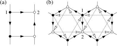
Figure 2: Configuration of $Z_{2}$ gauge fields $\{u_{jk}\}$ and $\{u^{\prime}_{jk}\}$ on (a) square and (b) hexagonal plaquettes; $u_{jk}=1$ if there is an arrow pointing from site $j$ to site $k$. The numbers 1 and 2 label the two inequivalent sites within a unit cell.

The question remains of what choices of $u_{jk}$, or equivalently the $Z_{2}$ fluxes $w_{p}$, give the lowest ground-state energy of the free fermion problem. Numerically, we find that such a state is attained when all hexagons are vortex free while all squares contain a $\pi$ flux:

$$w_{\varhexagon}=1,\quad\quad w_{\Square}=-1,$$ (5)

consistent with Lieb’s theorem. lieb A gauge choice which gives the desired plaquette fluxes without enlarging the unit cell is shown in Fig. 2. With this specific choice of $Z_{2}$ gauge field, the fermion spectrum can be obtained analytically using Fourier transformation.

In the weak-pairing regime to be discussed below, model (1) exhibits a gapless phase similar to the B phase of 2D Kitaev model. In order to explore possible topological insulators emerging from this critical phase, we consider the following single-ion perturbations:

$$\mathcal{H}_{1}=-\sum_{j}\mathbf{h}_{j}\cdot\bm{\sigma}_{j}+\lambda\sum_{j}\tau^{z}_{j}\hat{\mathbf{n}}\cdot\bm{\sigma}_{j}.$$ (6)

The first term is the Zeeman coupling to an external magnetic field $\mathbf{h}_{j}=\eta_{j}\mathbf{h}$, where the phase factor $\eta_{j}=\pm 1$ depends only on the $z$ coordinate of spin $j$, i.e. the field is constant within a given honeycomb plane. As mentioned previously, we shall consider two special cases in this paper: uniform field with $\eta_{j}=1$ and staggered field with $\eta_{j}=(-1)^{z_{j}}$. Since spins transform as $T\sigma^{\alpha}T^{-1}=-\sigma^{\alpha}$ under time-reversal $T$, the first term above explicitly breaks TRS.

The second term in Eq. (6) represents a spin-orbit-like interaction where $\lambda$ is an effective coupling constant, and $\hat{\mathbf{n}}$ is a unit vector specifying the local anisotropy axis. Such a coupling arises when the orbital basis $|\tau^{z}=\pm 1\rangle$ carries a nonzero orbital angular momentum $\mathbf{L}\sim\tau^{z}\hat{\mathbf{n}}$ which is parallel or antiparallel to the local anisotropy axis depending on $\tau^{z}=+1$ or $-1$, respectively. An explicit example is given by two degenerate orbitals with $t_{2g}$ symmetry, e.g. $|yz\rangle$ and $|zx\rangle$ in a tetragonal crystal field. By identifying $|\tau^{z}=\pm 1\rangle$ as $|yz\rangle\pm i|zx\rangle$, respectively, the orbital basis has a nonzero angular momentum pointing along the symmetry axis of the tetragonal field.

The effects of $\mathcal{H}_{1}$ can be studied following the perturbation treatments discussed in Ref. kitaev06, . Essentially, one constructs an effective Hamiltonian acting on the subspace which is free of vortex-type excitations. The first-order correction vanishes identically as both single-ion perturbations create $\pi$ fluxes on hexagons, baskaran07 whereas the second-order terms simply modify the nearest-neighbor exchange constants $J_{\alpha}$. Nontrivial corrections to the fermion spectrum arise at the third-order perturbation which involves multiple spin-orbital interactions, e.g.

$$(\tau^{z}_{j}\sigma^{x}_{j})(\tau^{z}_{k}\sigma^{y}_{k})\,\sigma^{z}_{l}=i(\tau^{z}_{j}\sigma^{x}_{j})(\tau^{z}_{k}\sigma^{y}_{k})(\tau^{z}_{l}\sigma^{x}_{l})(\tau^{z}_{l}\sigma^{y}_{l}).$$

Such terms introduce an effective second nearest-neighbor hopping for Majorana fermions

$$\mathcal{H}_{1}=\frac{i\kappa}{2}\sum_{jk}\eta\,u^{\prime}_{jk}c_{j}c_{k},$$ (7)

where $\kappa\sim\lambda^{2}h/J^{2}$ and $\eta=\pm 1$ is a constant within the plane containing sites $j$ and $k$. The additional second-neighbor $Z_{2}$ field $u^{\prime}_{jk}=-u^{\prime}_{kj}$ is shown by the dashed line in Fig. 2. Depending on the direction of $\hat{\mathbf{n}}$ and $\mathbf{h}$, the hopping amplitude $\kappa$ could take different values along inequivalent second-neighbor links. As the main purpose of this term is to introduce a spectral gap, to avoid unnecessary complications, we shall assume the symmetric case in the following discussion.

III Uniform magnetic field

We first discuss the ground state in the presence of a uniform magnetic field, i.e. $\eta_{j}=+1$ for all layers. As will be discussed below, the gapped phase at large fields is characterized by a $\pi_{2}$ Chern number corresponding to a multi-layer generalization of the 2D Kitaev model, and is topologically trivial in 3D (which generally is characterized by $\pi_{3}$ homotopy groups). This is mainly because the TRS essential to the existence of 3D topological insulators is explicitly broken by the uniform field. However, the critical phase in the case of small fields is interesting in itself and is similar to the gapless A-phase of ³He discussed in Ref. volovik, ; the gaplessness of both phases are topologically protected.

Since the original unit cell of the lattice is preserved by the $Z_{2}$ fields $u_{jk}$ and $u^{\prime}_{jk}$ shown in Fig. 2, we express the site index as $j=(\mathbf{r},s)$, where $\mathbf{r}$ denotes the position of the unit cell, and $s=1,2$ indicates the two inequivalent sites in a unit cell. With Fourier transformation $a_{\mathbf{k},s}=\sum_{\bf r}c_{\mathbf{r},s}\,e^{-i\mathbf{k}\cdot(\mathbf{r}+\mathbf{d}_{s})}/\sqrt{2N}$, where $\mathbf{d}_{s}$ is a basis vector and $N$ is the number of unit cells, the Hamiltonian becomes $\mathcal{H}=\mathcal{H}_{0}+\mathcal{H}_{1}=\frac{1}{2}\sum_{\mathbf{k}}\,\Psi^{\dagger}_{\mathbf{k}}\,H(\mathbf{k})\,\Psi_{\mathbf{k}}$, with $\Psi_{\mathbf{k}}=(a_{\mathbf{k},1},\,a_{\mathbf{k},2})^{T}$ and

$$H(\mathbf{k}) = \left(\begin{array}[]{cc}g(k_{z})+\Delta(\mathbf{k}_{\perp})&-if(\mathbf{k}_{\perp})\\ if(\mathbf{k}_{\perp})^{*}&-g(k_{z})-\Delta(\mathbf{k}_{\perp})\end{array}\right),$$

$$= {\rm Im}f(\mathbf{k}_{\perp})\,\tau^{x}+{\rm Re}f(\mathbf{k}_{\perp})\,\tau^{y}+\bigl{[}g(k_{z})\!+\!\Delta(\mathbf{k}_{\perp})\bigr{]}\,\tau^{z}.$$

For convenience, we have defined the following functions:

$$g(k_{z})=4J_{\parallel}\sin k_{z},\quad f(\mathbf{k}_{\perp})=2\sum_{\alpha=1}^{3}J_{\alpha}\,e^{i\mathbf{k}_{\perp}\cdot\bm{\delta}_{\alpha}},$$ (11)

$$\Delta(\mathbf{k}_{\perp})=8\kappa\,\sin\frac{k_{x}}{2}\,\Bigl{(}\cos\frac{\sqrt{3}k_{y}}{2}-\cos\frac{k_{x}}{2}\Bigr{)}.\quad$$

The three vectors $\bm{\delta}_{1,2}=(\frac{\pm 1}{2},\frac{-1}{2\sqrt{3}})$, and $\bm{\delta}_{3}=(0,\frac{1}{\sqrt{3}})$ connect nearest-neighbor sites in a honeycomb layer. In the following we shall focus on the emergent free fermion problem. The Pauli matrices $\tau^{\mu}$ appearing in the single-particle Hamiltonian now act on the sublattice index $s$ (not to be confused with orbital pseudospins).

The hermitian matrix $H(\mathbf{k})$ in Eq. (III) also satisfies

$$H^{T}(-\mathbf{k})=-H(\mathbf{k}),$$ (12)

which is the defining property of symmetry class D in Altland-Zirnbauer’s classification. az As 3D insulators in this class is topologically trivial, schnyder08 the gapped phase of Eq. (III) represents a trivial multilayer generalization of the 2D Kitaev model. Nonetheless, for small magnetic fields such that the second-neighbor hopping $\kappa\sim\lambda^{2}h$ is below a critical value $\kappa_{c}$, the fermion spectrum remains gapless in the weak-paring regime of the model. The corresponding critical phase is characterized by topologically protected Fermi points as we shall discuss below.

Diagonalizing Hamiltonian (III) yields a spectrum:

$$\epsilon_{\pm}(\mathbf{k})=\pm\sqrt{\bigl{[}g(k_{z})+\Delta(\mathbf{k}_{\perp})\bigr{]}^{2}+|f(\mathbf{k}_{\perp})|^{2}}.$$ (13)

When one of the in-plane coupling is much larger than the other two, e.g. $J_{z}\gg J_{x},J_{y}$, there is no solution to equation $f(\mathbf{k}_{\perp})=0$, and the spectrum is always gapped irrespective of the applied magnetic field. This phase corresponds to the A phase of the 2D Kitaev model, kitaev06 and is referred to in the following as the strong-pairing phase based on analogy with the $p$-wave topological superconductors. read00 On the other hand, in the weak-pairing regime of the model where the three in-plane couplings satisfy the triangle inequalities, kitaev06 the model displays a possible gapless phase as two solutions $\mathbf{k}^{*}_{\perp}$ exist for the equation $f(\mathbf{k}_{\perp})=0$. To be specific, we now concentrate on the symmetric case $J_{x}=J_{y}=J_{z}\equiv J$, where zeros of $f(\mathbf{k}_{\perp})$ are at the corners of the 2D hexagonal Brillouin zone $\mathbf{k}^{*}_{\perp}=(\pm\frac{4\pi}{3},0)$.

In contrast to the 2D Kitaev model where applying a magnetic field immediately opens an energy gap, kitaev06 spectrum (13) of the 3D model remains gapless when $\kappa$ is less than a critical strength $|\kappa|\leq\kappa_{c}.$ For symmetric in-plane couplings, we find $\kappa_{c}\equiv 2J_{\parallel}/3\sqrt{3}$ and the nodes of the spectrum $\epsilon_{\pm}(\mathbf{k})$ are located at

$$\begin{array}[]{llcl}&\mathbf{k}^{*}_{1,+}=\bigl{(}\frac{4\pi}{3},0,-\pi+\xi\bigr{)},&&\mathbf{k}^{*}_{1,-}=\bigl{(}\frac{4\pi}{3},0,-\xi\bigr{)},\\ &\mathbf{k}^{*}_{2,+}=\bigl{(}-\frac{4\pi}{3},0,\xi\bigr{)},&&\mathbf{k}^{*}_{2,-}=\bigl{(}-\frac{4\pi}{3},0,\pi-\xi\bigr{)},\end{array}\quad$$ (16)

where $\xi=\arcsin(\kappa/\kappa_{c})$. These Fermi points are topologically protected and are robust against weak perturbations. To see this, we first rewrite Hamiltonian (III) as $H(\mathbf{k})=\varepsilon_{+}(\mathbf{k})\,\hat{\mathbf{m}}(\mathbf{k})\!\cdot\!\bm{\tau}$, where $\hat{\mathbf{m}}(\mathbf{k})$ is a unit vector. A topological invariant characterizing the singularities of the spectrum is given by the winding number of mappings from a sphere $S^{2}$ enclosing the Fermi point $\mathbf{k}^{*}$ to the 2-sphere of the unit vector $\hat{\mathbf{m}}$: volovik

$$\nu=\int_{S^{2}}\frac{d^{2}A_{\rho}}{8\pi}\epsilon^{\mu\nu\rho}\,\hat{\mathbf{m}}\cdot\bigl{(}\partial_{\mu}\hat{\mathbf{m}}\times\partial_{\nu}\hat{\mathbf{m}}\bigr{)}.$$ (17)

The above definition corresponds to the second homotopy group $\pi_{2}(S^{2})=Z$, which characterizes point defects in an $O(3)$ spin field.mermin79

Examples of topologically nontrivial Fermi points are given by the spectra of Weyl Hamiltonian describing a massless spin-1/2 particle: $H_{\rm Weyl}=\pm ic\tau^{\mu}\partial_{\mu}$, where $c$ is the speed of light. volovik The plus and minus signs refer to left and right-handed particles, respectively. Using Eq. (17) the winding number of Weyl spinors can be readily computed, resulting $\nu=\pm 1$ for right and left-handed particles, respectively. Take left-handed Weyl spinor for example, the expectation value of its spin is parallel to its momentum: $\langle\bm{\tau}\rangle\parallel\mathbf{p}$. In the ground state with filled negative-energy states, Fermi point with $\nu=1$ thus looks like a magnetic monopole (a hedgehog) in momentum space. These singular points are robust in the sense that it is impossible to continuously deform a hedgehog into a uniform spin configuration (corresponding to the trivial case of $\nu=0$).

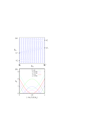
Figure 3: (Color online) (a) Projection of ground-state pseudospin $\langle\bm{\tau}\rangle=-\hat{\mathbf{m}}(\mathbf{k})$ on a face of the Brillouin zone. The two vertical edges of the face correspond to $K=(\frac{4\pi}{3},0,k_{z})$ and $K^{\prime}=(\frac{2\pi}{3},\frac{2\pi}{\sqrt{3}},k_{z})\equiv(-\frac{4\pi}{3},0,k_{z})$. The location of the four topologically non-trivial Fermi points are indicated by black arrows. (b) Dispersion along the $K^{\prime}$ edge of Brillouin zone for various $\kappa\sim\lambda^{2}h$. Upon increasing magnetic field $h$, the two Fermi points carrying opposite winding numbers move in opposite directions along the $K^{\prime}$ edge. At a critical field ($\kappa=\kappa_{c}$), the two singularities merge to form a new Fermi point with trivial winding number $\nu=0$ at $(-\frac{4\pi}{3},0,\frac{\pi}{2})$. The spectrum becomes gapped above $\kappa_{c}$.

To compute the winding number of Fermi points in our 3D model, we expand Hamiltonian (III) around the singular points, e.g.

$$H(\mathbf{k}^{*}_{1,\pm}+\mathbf{p})=-v_{\perp}p_{y}\tau^{x}-v_{\perp}p_{x}\tau^{y}\mp v_{\parallel}p_{z}\tau^{z},$$ (18)

where the Fermi velocities are $v_{\perp}=\sqrt{3}J$ and $v_{\parallel}\!=\!2(4J_{\parallel}^{2}-27\kappa^{2})^{1/2}$. The dispersion around these points has a conic singularity: $\varepsilon_{\pm}\!\approx\!\pm\sqrt{(v_{\perp}\mathbf{p}_{\perp})^{2}+(v_{\parallel}p_{z})^{2}}$. After rotation and mirror-inversion, Eq. (18) is essentially equivalent to the momentum-space Weyl Hamiltonian discussed above. The four Fermi points (16) form two pairs (labeled by $r=1,2$) of singularities with opposite winding numbers $\nu=\pm 1$. The ground-state configuration of pseudospin $\langle\bm{\tau}\rangle=-\hat{\mathbf{m}}(\mathbf{k})$ projected onto a face of the Brillouin zone is shown in Fig. 3(a). The two pairs of singularities are located at the two inequivalent edges $K$ and $K^{\prime}$ of the 3D Brillouin zone. Instead of a monopole-like configuration, vector field $\hat{\mathbf{m}}(\mathbf{k})$ in the vicinity of these Fermi points has a saddle-point-like singularity.

Although these Fermi points are topologically protected due to their nonzero winding numbers, a spectral gap can still be induced through mutual annihilation of Fermi points carrying opposite topological charges. This process is illustrated in Fig. 3. Take for example the two Fermi points on the $K^{\prime}$-edge of the Brillouin zone. Upon increasing magnetic field $h$, the two singularities characterized by winding numbers $\nu=\pm 1$ move toward each other along the $K^{\prime}$ edge, and eventually merge to form a new Fermi point when $\kappa$ reaches the critical $\kappa_{c}$. Because of the conservation of topological charge, the new Fermi point has a winding number $\nu=0$, hence is topologically trivial. Above the critical field, the spectrum is fully gapped.

It is also interesting to understand the critical B phase of Kitaev’s original 2D model from the perspective of topological winding number. As discussed in Ref. kitaev06, , the gaplessness of B phase is protected by TRS on the bipartite honeycomb lattice. This discrete symmetry essentially forces the unit vector $\hat{\mathbf{m}}(\mathbf{k}_{\perp})$ to lie in the $xy$ plane as $\tau^{z}$ terms in Eq. (III) is not allowed by TRS. For a planar unit vector $\hat{\mathbf{m}}$ whose tip lies on a circle $S^{1}$, the singularities are characterized by an integer topological invariant, also known as the vortex winding number, corresponding to $\pi_{1}(S^{1})=Z$. mermin79 The two Fermi poins in the B phase of Kitaev’s model can be viewed as vortices carrying opposite winding numbers $\nu=\pm 1$, respectively. In the presence of perturbations breaking the TRS, the vector $\hat{\mathbf{m}}$ now lives on a 2-sphere. Since $\pi_{1}(S^{2})=0$, singularities of the spectrum are then topologically trivial ($\pi_{2}$ characterization of 2D singularities is not well defined).

The gapped phase above the critical $\kappa_{c}$ represents a trivial generalization of the 2D Kitaev model in much the same way as the multilayer generalization of the IQH state. The topological properties of such systems are characterized by three spectral Chern numbers. kohmoto92 In our case, the nonzero topological invariant is given by the winding number of vector field $\hat{\mathbf{m}}(\mathbf{k}_{\perp};k_{z})$ which maps the in-plane hexagonal Brillouin zone (a 2-torus) to a unit 2-sphere:

$$\nu=\frac{1}{4\pi}\int dk_{x}dk_{y}\,\hat{\mathbf{m}}\cdot\bigl{(}\partial_{x}\hat{\mathbf{m}}\times\partial_{y}\hat{\mathbf{m}}\bigr{)}=\frac{\kappa}{|\kappa|}.$$ (19)

By treating $k_{z}$ as a parameter, Hamiltonian (III) has exactly the same form as that of the 2D Kitaev model. The first Chern number (19) of the corresponding ‘2D’ Hamiltonian $H_{k_{z}}(\mathbf{k}_{\perp})$ is given by $\nu={\rm sgn}\,\Delta_{k_{z}}$, kitaev06 where $\Delta_{k_{z}}=6\sqrt{3}(\kappa+\kappa_{c}\,\sin k_{z})$ is the effective gap parameter at corner $K$ of the hexagonal Brillouin zone. Therefore, as long as $|\kappa|>\kappa_{c}$, hence the system remains gapped, the winding number $\nu={\rm sgn}\kappa=\pm 1$ is independent of $k_{z}$, and the whole Brillouin zone is characterized by the same chirality.

IV Staggered magnetic field

The gapped phase discussed in the previous section is topologically trivial due to the absence of TRS. As discussed in Ref. schnyder08, , TRS is a prerequisite for the existence of 3D topological insulators. In this section, we show that one can introduce a gap to the fermion spectrum, while at the same time preserving an effective TRS, by subjecting the system to a staggered magnetic field, i.e. $\eta_{j}=(-1)^{z_{j}}$. Because the sign of the field alternates between successive honeycomb layers, a discrete symmetry emerges in our model system as Hamiltonian (6) is invariant under time-reversal $T$ followed by a lattice translation along $z$ axis. This additional symmetry manifests itself as a TRS in the auxiliary Majorana hopping problem. The mechanism proposed here is similar to Haldane’s model of realizing 2D quantum Hall effect without a net magnetic flux through the unit cells. haldane88

Due to the staggered field, the sign of second nearest-neighbor hopping $u^{\prime}_{jk}$ also alternates between successive honeycomb planes. This results in a staggered gap function $\pm\Delta(\mathbf{k}_{\perp})$, and a doubled unit cell along $z$ direction. We denote the fermion annihilation operators on the even and odd layers as $a_{\mathbf{r},s}$ and $b_{\mathbf{r},s}$, respectively, where subscript $s=1,2$ refers to the two inequivalent sites within a honeycomb plane. The Fourier-transformed Hamiltonian then reads $\mathcal{H}=\frac{1}{2}\sum_{\mathbf{k}}\Psi^{\dagger}_{\mathbf{k}}H(\mathbf{k})\Psi_{\mathbf{k}}$, with

$$H(\mathbf{k})=\left(\begin{array}[]{cccc}\Delta(\mathbf{k}_{\perp})&g(k_{z})&-if(\mathbf{k}_{\perp})&0\\ g(k_{z})&-\Delta(\mathbf{k}_{\perp})&0&-if(\mathbf{k}_{\perp})\\ if(\mathbf{k}_{\perp})^{*}&0&-\Delta(\mathbf{k}_{\perp})&-g(k_{z})\\ 0&if(\mathbf{k}_{\perp})^{*}&-g(k_{z})&\Delta(\mathbf{k}_{\perp})\end{array}\right)\quad\,\,\,\,$$ (24)

$$\,\,=\Delta(\mathbf{k}_{\perp})\tau^{z}\sigma^{z}\!+\!g(k_{z})\tau^{z}\sigma^{x}\!+\!{\rm Im}f(\mathbf{k}_{\perp})\tau^{x}\!+\!{\rm Re}f(\mathbf{k}_{\perp})\tau^{y},$$

and $\Psi_{\mathbf{k}}=\bigl{(}a_{\mathbf{k},1},b_{\mathbf{k}_{,}1},a_{\mathbf{k},2},b_{\mathbf{k},2}\bigr{)}^{T}$. The two sets of Pauli matrices $\tau^{\mu}$ and $\sigma^{\mu}$ now act on the sublattice $(1,2)$ and even-odd $(a,b)$ indices, respectively.

In addition to symmetry relation (12) shared by Hamiltonians describing free Majorana fermions, the hermitian matrix (24) also satisfies

$$\tau^{z}(i\sigma^{y})\,H^{T}(\mathbf{k})\,(-i\sigma^{y})\,\tau^{z}=H(-\mathbf{k}),$$ (25)

stemming from the generalized TRS. The extra $\tau^{z}$ factor can be gauged away by a $\pi/2$ rotation about the $\tau^{z}$ axis. Eq. (25) defines the symmetry property of DIII Hamiltonians in Altland-Zirnbauer’s classification. az As discussed in Ref. schnyder08, , a topological invariant can be defined for Hamiltonians in this symmetry class based on the block off-diagonal representation of the Hamiltonian, or more precisely, of the spectral projection operator. In fact, the same definition can be applied to classes of Hamiltonians which possess some form of chiral symmetry arising from either the sublattice symmetry or a combination of particle-hole and time-reversal symmetries. schnyder08

To compute the topological winding number of our model, we first bring Hamiltonian (24) into a block off-diagonal form through a series of unitary transformations. First, noting that the layered honeycomb lattice is bipartite in which nearest neighbors of one sublattice belong to the other one, we regroup fermions of the same sublattice into a block, e.g. $a_{\mathbf{k},1}$ and $b_{\mathbf{k},2}$. Mathematically this is achieved by interchanging the 2nd and 4th entries of $\Psi_{\mathbf{k}}$, the transformed Hamiltonian becomes

$$H(\mathbf{k})\to\alpha^{x}{\rm Im}f(\mathbf{k}_{\perp})+\alpha^{y}{\rm Re}f(\mathbf{k}_{\perp})+\alpha^{z}g(k_{z})+\beta\Delta(\mathbf{k}_{\perp}),\quad\,$$ (26)

where $\alpha^{\mu}$ and $\beta$ given by

$$\alpha^{\mu}=\gamma^{\mu}=\tau^{x}\sigma^{\mu},\quad\beta=\gamma^{0}=\tau^{z},$$ (27)

are the standard Dirac matrices. The second part of the unitary transformation is a $\pi/2$ rotation about the new $\tau^{x}$ axis, which transforms $\tau^{z}\to\tau^{y}$, hence

$$H(\mathbf{k})\to\left(\begin{array}[]{cc}0&D(\mathbf{k})\\ D^{\dagger}(\mathbf{k})&0\end{array}\right),$$ (30)

where the upper right block is

$$D(\mathbf{k})=\left(\begin{array}[]{cc}g(k_{z})-i\Delta(\mathbf{k}_{\perp})&-if(\mathbf{k}_{\perp})\\ if(\mathbf{k}_{\perp})^{*}&-g(k_{z})-i\Delta(\mathbf{k}_{\perp})\end{array}\right).$$ (33)

Noting that $f(-\mathbf{k}_{\perp})=f(\mathbf{k}_{\perp})^{*}$, and $\Delta(\mathbf{k}_{\perp})$, $g(k_{z})$ are odd functions of $\mathbf{k}$, matrix (33) satisfies a symmetry $D^{T}(\mathbf{k})=-D(-\mathbf{k})$. The block off-diagonal form of the Hamiltonian implies that $\epsilon(\mathbf{k})^{2}=D^{\dagger}(\mathbf{k})D(\mathbf{k})$, which gives rise to a fermion spectrum

$$\epsilon_{\pm}(\mathbf{k})=\pm\sqrt{\Delta(\mathbf{k}_{\perp})^{2}+g(k_{z})^{2}+\bigl{|}f(\mathbf{k}_{\perp})\bigr{|}^{2}}.$$ (34)

Due to the effective TRS (25), the spectrum is double degenerate at each wavevector $\mathbf{k}$, except at possible Fermi points. It is worth noting that, contrary to the uniform field case, the staggered field immediately opens an energy gap to the spectrum in the weak-pairing phase of the model.

The topological properties of the quantum ground state (occupied Bloch states) in the gapped phase is captured by the following $Q$ matrix: schnyder08

$$Q(\mathbf{k})=\left(\begin{array}[]{cc}0&q(\mathbf{k})\\ q^{\dagger}(\mathbf{k})&0\end{array}\right),\quad q(\mathbf{k})=\frac{D(\mathbf{k})}{\epsilon_{+}(\mathbf{k})}.$$ (37)

In fact $Q(\mathbf{k})$ represents a ‘simplified’ Hamiltonian obtained by assigning an energy $\epsilon=-1$ to all occupied states and $\epsilon=+1$ to all empty bands of Hamiltonian $H(\mathbf{k})$. schnyder08 ; qi09 As long as the system is in the same gapped phase, one can continuously deform the model such that $H(\mathbf{k})$ gradually transforms to the simplified form $Q(\mathbf{k})$. Not surprisingly, the $Q$ matrix is related to the spectral operator via $Q(\mathbf{k})=1-2P(\mathbf{k})$. schnyder08

It is easy to see that the block matrix $q$ satisfies

$$q^{\dagger}(\mathbf{k})\,q(\mathbf{k})=1,\quad q^{T}(\mathbf{k})=-q(-\mathbf{k}),$$ (38)

as expected for a DIII class Hamiltonian. The topological invariant characterizing the ground state is defined as the integer winding number of mapping $q:T^{3}\to U(2)$, schnyder08 ; volovik

$$\nu=\int\frac{d^{3}k}{24\pi^{2}}\epsilon^{\mu\nu\rho}{\rm tr}\bigl{[}(q^{-1}\partial_{\mu}q)(q^{-1}\partial_{\nu}q)(q^{-1}\partial_{\rho}q)\bigr{]},$$ (39)

where the integral is over the three-dimensional Brillouin zone, which is essentially a 3-torus $T^{3}$. For DIII class Hamiltonians, the winding number $\nu$ can take on an arbitrary integer, each labels a unique topological class of the quantum ground state.

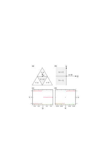
Figure 4: (Color online) (a) Phase diagram in the plane of $J_{x}+J_{y}+J_{z}=$ const. The shaded triangle corresponds to the region where the in-plane couplings satisfy the triangle inequalities. In the absence of staggered field $\kappa=0$, the shaded area represents a critical phase with zero energy gap. We define a parameter $\delta=2J_{x}-J_{z}$ along the $J_{x}=J_{y}$ line specifying the distance from the phase boundary. (b) Phase diagram as a function of distance $\delta$ and field strength $\kappa$. Panels (c) and (d) Numerical evaluation of the winding number $\nu$ as a function of $\delta$ and $\kappa$, respectively. The field strength $\kappa=\pm 0.02J_{z}$ in the calculation of panel (c), whereas we set $J_{x}=J_{y}=J_{z}\equiv J$ and $\kappa$ is measured in units of $J$ in (d).

The value of the topological winding number $\nu$ can only change in the presence of a quantum phase transition, which is usually accompanied by a vanishing bulk gap. In our case, noting that $g(0)=0$, a prerequisite for spectrum (34) to be gapless is that the in-plane couplings satisfy the triangle inequalities $|J_{z}|\leq|J_{x}|+|J_{y}|$, and so on [see Fig. 4(a)], such that solutions exist for $f(\mathbf{k}_{\perp})=0$ (the weak-paring regime of the model). In the absence of magnetic field $\kappa=h=0$, the triangle inequalities thus define a critical phase with gapless fermionic excitations. For convenience, we use $\delta$ to denote the ‘distance’ from the boundary of the critical phase. For example $\delta\equiv 2J_{x}-J_{z}$ along the $J_{x}=J_{y}$ line shown in Fig. 4(a). We numerically compute the winding number $\nu$ using definition (39) for various gapped phases of the model Hamiltonian; the resulting phase diagram as a function of $\delta$ and $\kappa$ is summarized in Fig. 4(b).

At the phase boundary defined by $\kappa=0$ and $\delta=0$, the system undergoes a quantum phase transition of a topological nature. Fig. 4(c) shows numerical evaluation of the winding number $\nu$ as a function of $\delta=2J_{x}-J_{z}$ in the presence of a staggered field such that $|\kappa|=0.02J_{z}$. Depending on the sign of $\kappa$, the winding number jumps from $\nu=0$ to $\nu=\pm 1$ when $\delta$ crosses the phase boundary from the topologically trivial phase (corresponding to the A phase in 2D Kitaev model). On the other hand, for systems inside the critical phase ($\delta<0$), the winding number jumps from $\nu=-1$ to $\nu=+1$ as $\kappa$ changes sign.

The nontrivial winding number of the quantum ground state can also be understood from the topological properties of the singular (Dirac) points in the fermion spectrum. To simplify the discussion, we focus on the symmetric case $J_{x}=J_{y}=J_{z}\equiv J$, where zeros of spectrum (34) in the $\kappa\to 0$ limit are at

$$\begin{array}[]{lcl}\mathbf{k}^{*}_{1}=(\frac{4\pi}{3},0,0),&&\mathbf{k}^{*}_{2}=(-\frac{4\pi}{3},0,0).\end{array}$$ (41)

In the vicinity of these two points, the fermions obey a Dirac-like Hamiltonian [c.f. Eq. (26)]

$$H(\mathbf{k}^{*}+\mathbf{p})=\alpha^{\mu}\tilde{p}_{\mu}+m\beta,$$ (42)

where the scaled momentum and mass term are

$$\begin{array}[]{c}\tilde{\mathbf{p}}_{\perp}=\sqrt{3}J(p_{y},\mp p_{x}),\quad\tilde{p}_{z}=4J_{\perp}p_{z},\\ \\ m=\Delta(\mathbf{k}^{*}_{s})=\pm 6\sqrt{3}\kappa.\end{array}$$ (46)

The plus and minus signs in the expression of $m$ correspond to $\mathbf{k}^{*}_{1}$ and $\mathbf{k}^{*}_{2}$, respectively. The spectrum of (42) given by $\epsilon_{\pm}=\pm\sqrt{\tilde{p}^{2}+m^{2}}$ is two-fold degenerate at each $\mathbf{p}$. As discussed above, a $\pi/2$ rotation about $\tau^{x}$ brings the Dirac mass into a chiral mass term, i.e. $\beta\to i\gamma^{5}\beta$. The transformed Hamiltonian $H=\alpha_{\mu}\tilde{p}_{\mu}-i\beta\gamma^{5}m$ is in a block off-diagonal form with $D=\tilde{\mathbf{p}}\cdot\bm{\sigma}-im$. The $q$ matrix of the spectral projector is then given by

$$q(\mathbf{k}^{*}+\mathbf{p})=\frac{\tilde{\mathbf{p}}\cdot\bm{\sigma}-im}{\sqrt{\tilde{p}^{2}+m^{2}}}.$$ (47)

Eqs. (42) and (47) can be viewed as a continuum approximation to the low-energy physics of the model system. A direct evaluation using Eq. (39) yields a winding number

$$\nu=\pm\frac{1}{2}\frac{m}{|m|},$$ (48)

with $\pm$ sign refering to $\mathbf{k}^{*}_{1}$ and $\mathbf{k}^{*}_{2}$ points, respectively. Note that when evaluating $\nu$ using the continuum description, we have extended the domain of integration to a 3-sphere in Eq. (39). The appearance of a half-integer $\nu$ is an artifact of the continuum description; the winding number is modified once contributions from high-energy Bloch states (away from the Dirac point in the Brillouin zone) are properly included. Since the mass term has opposite sign at the two Dirac points, $m(\mathbf{k}^{*}_{1})=-m(\mathbf{k}^{*}_{2})$, we obtain $\nu_{1}=\nu_{2}=\frac{1}{2}{\rm sgn}\,\kappa$. Interestingly, the sum of these two winding numbers $\nu=\nu_{1}+\nu_{2}$ reproduces the topological invariant of the lattice model.

As recently pointed out in Ref. beri09, , stable Fermi lines generally appears in 3D topological superconductors described by Hamiltonians belonging to classes CI or DIII. An extended phase diagram of a lattice CI model schnyder09b indeed shows regions of gapless phase with topologically stable Fermi lines. beri09 Here we show that such Fermi lines are also possible in our DIII Hamiltonian (24).

To this end, we consider perturbations which break the sublattice symmetry by introducing different second-neighbor hoppings $\kappa$ on the two inequivalent sites of the lattice: $\kappa_{1,2}=\kappa\pm\delta\kappa$. In the vicinity of the Dirac points (41), the asymmetric coupling results in an additional term of the off-diagonal block matrix

$$D=\tilde{\mathbf{p}}\cdot\bm{\sigma}-im-i\mu\sigma^{z},\quad\quad\mu=6\sqrt{3}\,\delta\kappa.$$ (49)

The corresponding spectrum $\epsilon^{2}=\tilde{p}_{z}^{2}+\bigl{(}\mu-\sqrt{m^{2}+\tilde{p}_{\perp}^{2}}\bigr{)}^{2}$ has a Fermi line specified by

$$\tilde{p}_{\perp}=\sqrt{\mu^{2}-m^{2}},\quad\quad\tilde{p}_{z}=0,$$ (50)

when $\mu>m$. Finally, we point out that introducing a similar asymmetric hopping $\delta\kappa$ in the case of uniform field results in a Fermi surface in the weak-pairing regime.

V Gapless Surface Majorana fermions

Analogous to the gapless chiral edge modes in the non-Abelian phase of 2D Kitaev model, kitaev06 the nontrivial topology of the $\nu=\pm 1$ quantum ground state in our 3D model manifests itself through the appearance of gapless Majorana fermions at the sample surface. To study the properties of these surface modes, we solve the Majorana hopping problem (4) and (7) in a finite geometry with periodic boundary conditions along $x$ and $z$ directions and open boundary condition along $y$ direction. We assume that the $x$-axis is parallel to the zigzag direction of the honeycomb lattice. As Fig. 5 shows, in addition to gapped states in the bulk, the spectrum of a finite system contains additional surface modes crossing the bulk gap.

The properties of these surface states can be understood analytically using the edge modes of 2D Kitaev model, whose existence has been demonstrated in Ref. kitaev06, . These boundary modes are confined to the edge of the honeycomb lattice and possess a definite chirality depending on the sign of magnetic field $h$. Without loss of generality, we assume $\kappa\sim\lambda^{2}h>0$, hence $\epsilon_{\perp}(k_{x})>0$ for positive $k_{x}$ in the 1D Brillouin zone. The Hamiltonian describing the edge states is given by

$$\mathcal{H}_{\rm edge}=\frac{1}{2}\sum_{k_{x}}\epsilon_{\perp}(k_{x})\,\chi(-k_{x})\,\chi(k_{x}),$$ (51)

where $\chi(k_{x})$ and $\chi(-k_{x})=\chi^{\dagger}(k_{x})$ for $k_{x}>0$ are annihilation and creation operators, respectively, of the Majorana edge modes. The spectrum of the edge states has the form $\epsilon_{\perp}(k_{x})\approx 12\kappa\sin k_{x}$ in the vicinity of the 1D Fermi point $k^{*}_{x}=\pi$, and gradually merges with the bulk spectrum as $k_{x}$ moves away from $k^{*}_{x}$. kitaev06

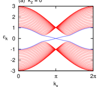
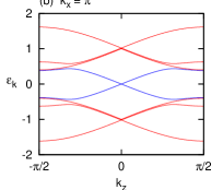
Figure 5: (Color online) Spectrum of a finite system with $L=10$ layers along $y$ direction. We consider the symmetric case with $J_{x}=J_{y}=J_{z}\equiv J$. Coupling constant along vertical links is set to $J_{\parallel}=0.35J$, and the strength of the uniform field is $\kappa=0.05J$. Panels (a) and (b) show dispersion along $k_{x}$ and $k_{z}$ directions, respectively, of the 2D surface Brillouin zone.

It is interesting to note that the $J_{\parallel}=0$ limit of the 3D model (1) can be viewed as a collection of decoupled honeycomb layers. Due to the staggered magnetic field, the edge states on even and odd numbered layers have opposite chirality $\nu=\pm{\rm sgn}\,\kappa$; the corresponding quasiparticle operators are denoted as $\chi_{+}(k_{x},2n)$ and $\chi_{-}(k_{x},2n+1)$, respectively. The ensemble of the edge modes is described by Hamiltonian:

$$\mathcal{H}_{\perp}=\frac{1}{2}\sum_{n}\sum_{k_{x}}\epsilon_{\perp}(k_{x})\bigl{[}\chi_{+}(-k_{x},2n)\chi_{+}(k_{x},2n)$$

$$-\chi_{-}(-k_{x},2n+1)\chi_{-}(k_{x},2n+1)\bigr{]}.$$ (52)

For odd-numbered layers, the quasiparticle annihilation operator is given by $\chi_{-}(k_{x},2n+1)$ with negative $k_{x}$. A nonzero $J_{\parallel}$ introduces coupling between adjacent layers:

$$\mathcal{H}_{\parallel}=iJ_{\parallel}\sum_{n}\sum_{k_{x}}\bigl{[}\chi_{-}(-k_{x},2n+1)\chi_{+}(k_{x},2n)$$

$$+\chi_{+}(-k_{x},2n)\chi_{-}(k_{x},2n-1)\bigr{]}.$$ (53)

After Fourier transformation with respect to $z$ coordinate, we obtain the Hamiltonian for surface modes

$$\mathcal{H}_{\rm surf}=\frac{1}{2}\sum_{k_{x},k_{z}}\psi^{\dagger}_{k_{x},k_{z}}\bigl{[}\epsilon_{\perp}(k_{x})\sigma^{z}+\epsilon_{\parallel}(k_{z})\sigma^{x}\bigr{]}\psi_{k_{x},k_{z}},$$ (54)

where $\psi_{k_{x},k_{z}}=\bigl{(}\chi_{+}(k_{x},k_{z}),\chi_{-}(k_{x},k_{z})\bigr{)}^{T}$, and the off-diagonal coupling $\epsilon_{\parallel}(k_{z})=2J_{\parallel}\sin k_{z}$. The spectrum can be easily obtained $\epsilon_{\rm surf}=\bigl{(}\epsilon_{\parallel}^{2}+\epsilon_{\perp}^{2}\bigr{)}^{1/2}$. Consistent with the numerical calculation shown in Fig. 5, the surface spectrum has a conic singularity at the 2D Fermi point $(k^{*}_{x},k^{*}_{z})=(\pi,0)$.

In the continuum approximation, the low-energy surface modes close to the 2D Fermi point obeys a gapless Dirac-like Hamiltonian $H_{\rm Dirac}=-i(u_{\perp}\sigma^{z}\partial_{x}+u_{\parallel}\sigma^{x}\partial_{z})$. The existence of gapless surface Majorana modes is a direct consequence of the nontrivial ground-state topology when the 3D bulk sample is terminated by a 2D boundary. callan85 ; fradkin86 Due to its topological nature, the surface Dirac cone is stable against perturbations respecting the effective TRS.

VI Discussion

To summarize, we have constructed an interacting bosonic model on a three-dimensional layered honeycomb lattice which displays topologically nontrivial ground states. Our approach is based on the $\Gamma$-matrix generalization of Kitaev’s original spin-1/2 model. levin03 ; hamma05 ; yao09 ; wu09 ; ryu09 ; nussinov09 We show that the ground state in the weak-pairing phase remains gapless in the presence of a small magnetic field. The fermion spectrum of this critical phase is characterized by four topologically protected Fermi points. Upon increasing the field strength, Fermi points with opposite winding numbers move toward each other and eventually annihilate at a critical field, signaling the transition into a topologically trivial phase with a gapped spectrum.

On the other hand, with the sign of magnetic field staggered along successive layers, the bulk spectrum of the weak-pairing phase immediately acquires a gap. An effective TRS is restored thanks to the staggering of the magnetic field. The corresponding quantum ground state is characterized by an integer winding invariant and possesses nontrivial topological properties, a manifestation of which is the appearance of protected gapless surface Majorana modes when the sample is terminated by a two-dimensional surface.

It is worth noting that our model provides an alternative example in which a 3D topological insulator emerges from an interacting bosonic Hamiltonian. More importantly, the TRS essential to the existence of 3D topological insulators is realized in our model through a generic physical mechanism, instead of relying on special symmetries of the $\Gamma$-matrix representation in the recently proposed diamond-lattice model. ryu09 ; wu09 We also remark that despite the experimental difficulty of realizing the Kitaev model and its variants, the study of these exactly solvable models has enriched our understanding of the physics of topological phases. Finally, we would like to point out that it remains unclear whether an emergent topological insulator can be realized in a spin-1/2 Kitaev model on a 3D trivalent lattice.

- (1) D. J. Thouless, M. Kohmoto, M. P. Nightingale, and M. den Nijs, Phys. Rev. Lett. 49, 405 (1982).
- (2) J. E. Avron, R. Seiler, and B. Simon, Phys. Rev. Lett. 51, 51 (1983).
- (3) M. Kohmoto, Annals of Physics 160, 428 (1985).
- (4) X.-G. Wen, Quantum Field Theory of Many-Body Systems, Oxford University Press (2004).
- (5) G. E. Volovik, The Universe in a Helium Droplet, The International Series of Monographs on Physics Vol. 117 Oxford University Press, New York (2000).
- (6) C. L. Kane and E. J. Mele, Phys. Rev. Lett. 95, 146802 (2005); Phys. Rev. Lett. 95, 226801 (2005).
- (7) B. A. Bernevig, S. C. Zhang, Phys. Rev. Lett. 96, 106802 (2006); B. A. Bernevig, T. L. Hughes, S. C. Zhang, Science 314, 1757 (2006).
- (8) J. E. Moore and L. Balents, Phys. Rev. B 75, 121306 (2007).
- (9) R. Roy, Phys. Rev. B 79, 195321 (2009).
- (10) L. Fu, C. L. Kane, and E. J. Mele, Phys. Rev. Lett. 98, 106803 (2007).
- (11) L. Fu and C. L. Kane, Phys. Rev. B 76, 045302 (2007).
- (12) R. Roy, Phys. Rev. B 79, 195322 (2009).
- (13) M. König, S. Wiedmann, C. Bruene, A. Roth, H. Buhmann, L. W. Molenkamp, X.-L. Qi, and S.-C. Zhang, Science 318, 766 (2007).
- (14) D. Hsieh, D. Qian, L. Wray, Y. Xia, Y. Hor, R. J. Cava, and M. Z. Hasan, Nature 452, 970 (2008).
- (15) Y. Xia, D. Qian, D. Hsieh, L. Wray, A. Pal, H. Lin, A. Bansil, D. Grauer, Y. S. Hor, R. J. Cava, and M. Z. Hasan, Nature Phys. 5, 398 (2009).
- (16) P. Roushan, J. Seo, C. V. Parker, Y. S. Hor, D. Hsieh, D. Qian, A. Richardella, M. Z. Hasan, R. J. Cava, and A. Yazdani, Nature 460, 1106 (2009).
- (17) Y. L. Chen, J. G. Analytis, J.-H. Chu, Z. K. Liu, S.-K. Mo, X. L. Qi, H. J. Zhang, D. H. Lu, X. Dai, Z. Fang, S. C. Zhang, I. R. Fisher, Z. Hussain, Z.-X. Shen, Science 325, 178 (2009).
- (18) A. P. Schnyder, S. Ryu, A. Furusaki, and A. W. W. Ludwig, Phys. Rev. B 78, 195125 (2008); AIP Conf. Proc. 1134, 10 (2009).
- (19) A. Yu Kitaev, AIP Conf. Proc. 1134, 22 (2009).
- (20) X.-L. Qi, T. L. Hughes, and S.-C. Zhang, Phys. Rev. B 78, 195424 (2008).
- (21) G. Jackeli and G. Khaliullin, Phys. Rev. Lett. 102, 017205 (2009).
- (22) A. Shitade, H. Katsura, J. Kunes, X.-L. Qi, S.-C. Zhang, N. Nagaosa, Phys. Rev. Lett. 102, 256403 (2009).
- (23) S. Raghu, X.-L. Qi, C. Honerkamp, S.-C. Zhang, Phys.Rev.Lett. 100, 156401 (2008).
- (24) K. Sun, H. Yao, E. Fradkin, and S. A. Kivelson, Phys. Rev. Lett. 103, 046811 (2009)
- (25) Yi Zhang, Ying Ran, and A. Vishwanath, Phys. Rev. B 79, 245331 (2009).
- (26) A. Yu Kitaev, Ann. Phys. 321, 2 (2006).
- (27) A. Yu Kitaev, Ann. Phys. 303, 2 (2003).
- (28) S. Yang, D. L. Zhou, and C. P. Sun, Phys. Rev. B 76, 180404 (2007).
- (29) H. Yao and S. A. Kivelson, Phys. Rev. Lett. 99, 247203 (2007).
- (30) T. Si and Y. Yu, arXiv.0709.1302 (2007).
- (31) T. Si and Y. Yu, Nucl. Phys. B 803, 428 (2008).
- (32) S. Mandal and N. Surendran, Phys. Rev. B 79, 024426 (2009).
- (33) G.-W. Chern, unpublished.
- (34) M. Levin and X.-G. Wen, Phys. Rev. B 67, 245316 (2003).
- (35) A. Hamma, P. Zanardi1, and X.-G. Wen, Phys. Rev. B 72, 035307 (2005).
- (36) H. Yao, S.-C. Zhang, and S. A. Kivelson, Phys. Rev. Lett. 102, 217202 (2009).
- (37) S. Ryu, Phys. Rev. B 79, 075124 (2009).
- (38) C. Wu, D. Arovas, and H.-H. Hung, Phys. Rev. B 79, 134427 (2009).
- (39) Z. Nussinov and G. Ortiz, Phys. Rev. B 79, 214440 (2009).
- (40) A. Altland and M. R. Zirnbauer, Phys. Rev. B 55, 1142 (1997).
- (41) K. I. Kugel and D. I. Khomskii, Sov. Phys. Usp. 231, 25 (1982).
- (42) E. H. Lieb, Phys. Rev. Lett. 73, 2158 (1994).
- (43) G. Baskaran, S. Mandal, and R. Shankar, Phys. Rev. Lett. 98, 247201 (2007).
- (44) N. Read and D. Green, Phys. Rev. B 61, 10267 (2000).
- (45) N. D. Mermin, Rev. Mod. Phys. 51, 591 (1979).
- (46) M. Kohmoto, B. I. Halperin, and Y.-S. Wu, Phys. Rev. B 45, 13488 (1992).
- (47) F. D. M. Haldane, Phys. Rev. Lett. 61, 2015 (1988).
- (48) X. L. Qi, T. L. Hughes, and S. C. Zhang, arXiv:0908.3550 (unpublished).
- (49) B. Béri, arXiv:0909.5680 (unpublished).
- (50) A. P. Schnyder, S. Ryu, and A. W. W. Ludwig, Phys. Rev. Lett. 102, 196804 (2009).
- (51) C. G. Callan, Jr. and J. A. Harvey, Nucl. Phys. B 250, 427 (1985).
- (52) E. Fradkin, E. Dagotto, and D. Boyanovsky, Phys. Rev. Lett. 57, 2967 (1986).