Vacuum energy between a sphere and a plane at finite temperature

Abstract

We consider the Casimir effect for a sphere in front of a plane at finite temperature for scalar and electromagnetic fields and calculate the limiting cases. For small separation we compare the exact results with the corresponding ones obtained in proximity force approximation. For the scalar field with Dirichlet boundary conditions, the low temperature correction is of order $T^{2}$ like for parallel planes. For the electromagnetic field it is of order $T^{4}$. For high temperature we observe the usual picture that the leading order is given by the zeroth Matsubara frequency. The non-zero frequencies are exponentially suppressed except for the case of close separation.

I Introduction

By now, the Casimir force between a sphere and a plane was calculated using the functional determinant (or TGTG- or T-matrix-) representation and, for scalar field, numerically by the world line methods, and, of course, in the Proximity Force Approximation (PFA). The extension of these methods to finite temperature is in its very beginning. Even for the PFA we did not find in literature a representation at finite temperature, although the calculation is quite simple. Recently Weber:2009dp ; Gies:2009nn , using the world line method, the temperature dependence was studied and an interesting interplay between geometry and temperature was observed. Using the functional determinant representation in Durand2009 a partly numerical, partly analytical study at medium and large separation was represented where also dielectric materials were included. It must be mentioned that the corrections beyond PFA are a topic of actual interest also for high precision measurements of the Casimir force where it is necessary to know the temperature corrections at small separation.

In this paper we calculate the free energy at finite temperature for a sphere in front of a plane for conductor boundary conditions using the functional determinant method which gives the exact result. We pay special attention to the case of small separation and to the limiting cases of low and high temperature. Also, for small separation we establish the relation to the Proximity Force Approximation (PFA) and determine where it is applicable.

The paper is organized as follows. In the next section we prepare the necessary formulas of the functional determinant representation. In sections 3 and 4 we calculate the temperature dependent part of the free energy at small separation by both methods, PFA and the functional determinant method. In sections 5 and 6 we derive the low and high temperature expansions using the functional determinant method. Finally, the results are discussed in section 7.

Throughout the paper we use units with $\hbar=c=k_{\rm B}=1$.

II Basic formulas

In this section we collect the formulas we need for the free energy in sphere-plane geometry. For the free energy we use the standard Matsubara-representation. For the interaction energy between a sphere and a plane we use it together with the functional determinant representation,

$${\cal F}=\frac{T}{2}\sum_{n=-\infty}^{\infty}{\rm Tr}\ln\left(1-\mathbf{M}(\xi_{n})\right),$$ (1)

where $\xi_{n}=2\pi Tn$ are the Matsubara frequencies. At zero temperature, the Matsubara sum becomes an integration, $T\sum_{n=-\infty}^{\infty}\to\int_{-\infty}^{\infty}\frac{d\xi}{2\pi}$ with $\xi_{n}\to\xi$ and the free energy turns into the vacuum energy,

$$E_{0}=\frac{1}{2}\int_{-\infty}^{\infty}\frac{d\xi}{2\pi}\ {\rm Tr}\ln\left(1-\mathbf{M}(\xi)\right).$$ (2)

In these formulas, $\mathbf{M}(\xi)$ is a matrix in the orbital momentum indices $l$ and $l^{\prime}$,

$$M_{l,l^{\prime}}(\xi)=d_{l}(\xi R)\sqrt{\frac{\pi}{4\xi L}}\sum_{l^{\prime\prime}=|l-l^{\prime}|}^{l+l^{\prime}}K_{\nu^{\prime\prime}}(2\xi L)\,H_{ll^{\prime}}^{l^{\prime\prime}}\,\,.$$ (3)

For Dirichlet boundary conditions on the sphere,

$$d_{l}(\xi)=\frac{I_{\nu^{\prime}}(\xi)}{K_{\nu}(\xi)}$$ (4)

results from the scattering T-matrix. In these formulas, $I_{l+1/2}(x)$ and $K_{l+1/2}(x)$ are the modified Bessel functions. The geometry is shown in Fig. 1. We introduced the notations $\nu=l+1/2$, $\nu^{\prime}=l^{\prime}+1/2$ and $\nu^{\prime\prime}=l^{\prime\prime}+1/2$, which will be used throughout the paper.

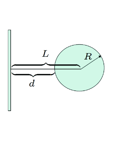
Figure 1: The configuration of a sphere in front of a plane.

The above formulas can be found in the original papers on the functional determinant method WIRZBA2006 , Emig:2007cf . Here we follow the notations used in BORDAG2008C and in BKMM . The factors $H_{ll^{\prime}}^{l^{\prime\prime}}$ in 3 result from the translation formulas. Their explicit form is

$$H_{ll^{\prime}}^{l^{\prime\prime}} = \sqrt{(2l+1)(2l^{\prime}+1)}(2l^{\prime\prime}+1)$$ (9)

$$\times\left(\begin{array}[]{ccc}l&l^{\prime}&l^{\prime\prime}\\ 0&0&0\end{array}\right)\left(\begin{array}[]{ccc}l&l^{\prime}&l^{\prime\prime}\\ m&-m&0\end{array}\right),$$

where the parentheses denote the $3j$-symbols. For Neumann boundary conditions on the sphere we have to substitute $d_{l}(x)$ by

$$d^{\rm N}_{l}(\xi)=\frac{\left(I_{\nu^{\prime}}(\xi)/\sqrt{\xi}\right)^{\prime}}{\left(K_{\nu}(\xi)/\sqrt{\xi}\right)^{\prime}}$$ (10)

and for Neumann boundary conditions on the plane we have to reverse the sign in the logarithm in 1.

For the electromagnetic field the matrix $\mathbf{M}$ acquires indices for the two polarizations, which correspond to the TE and the TM modes in spherical geometry,

$$\mathbb{M}_{l,l^{\prime}} = \sqrt{\frac{\pi}{4\xi L}}\sum_{l^{\prime\prime}=|l-l^{\prime}|}^{l+l^{\prime}}K_{\nu^{\prime\prime}}(2\xi L)H_{ll^{\prime}}^{l^{\prime\prime}}\,$$ (16)

$$\times\left(\begin{array}[]{cc}\Lambda_{l,l^{\prime}}^{l^{\prime\prime}}&\tilde{\Lambda}_{l,l^{\prime}}\\ \tilde{\Lambda}_{l,l^{\prime}}&\Lambda_{l,l^{\prime}}^{l^{\prime\prime}}\end{array}\right)\left(\begin{array}[]{cc}d^{\rm TE}_{l}(\xi R)&0\\ 0&-d^{\rm TM}_{l}(\xi R)\end{array}\right)\,.$$

with the factors

$$\Lambda_{ll^{\prime}}^{l^{\prime\prime}} = \frac{\frac{1}{2}\left[l^{\prime\prime}(l^{\prime\prime}+1)-l(l+1)-l^{\prime}(l^{\prime}+1)\right]}{\sqrt{l(l+1)l^{\prime}(l^{\prime}+1)}}\,,$$

$$\tilde{\Lambda}_{ll^{\prime}} = \frac{2m\xi L}{\sqrt{l(l+1)l^{\prime}(l^{\prime}+1)}}$$ (17)

which follow from the translation formulas for the vector field. The factors resulting from the scattering T-matrices are

$$d^{\rm TE}_{l}(\xi R)=\frac{I_{\nu^{\prime}}(\xi R)}{K_{\nu}(\xi R)}\,,$$ (18)

which is the same as for the scalar field with Dirichlet boundary conditions, and, for the TM-mode,

$$d^{\rm TM}_{l}(\xi R)=\frac{\left(I_{\nu^{\prime}}(\xi R)\sqrt{\xi R}\right)^{\prime}}{\left(K_{\nu}(\xi R)\sqrt{\xi R}\right)^{\prime}}\,.$$ (19)

When inserting these expressions into 1 or 2, the trace must be taken also over the polarizations. More details are given in BORDAG2009C .

III The PFA at finite temperature

In order to discuss the free energy at small separation which is the relevant scale for PFA we first define the corresponding temperature regions of interest. These are

$$\begin{array}[]{lrrrrr}\mbox{1. low temperature:}&dT&\ll&RT&\ll&1\,,\\ \mbox{2. medium temperature:~{}~{}~{}~{}}&dT&\ll&1&\ll&RT\,,\\ \mbox{3. high temperature:}&1&\ll&dT&\ll&RT\,.\end{array}$$ (20)

In each case $d\ll R$ holds. Further we introduce

$$\varepsilon=\frac{d}{R}$$ (21)

as small parameter.

Below we consider the PFA at finite temperature in some more detail as in Bordag:2001qi , section 5.1.2. We do this for the electromagnetic field with conductor boundary conditions. For that, first we need to remember the free energy ${\cal F}_{||}$ per unit area for two parallel planes. It can be obtained in several ways, for instance as special case from the general formula 1

$${\cal F}_{||}(d,T)=T\sum_{n=-\infty}^{\infty}\,\int\frac{d\mathbf{k}}{(2\pi)^{2}}\,\ln\left(1-e^{-2d\sqrt{\xi_{n}^{2}+\mathbf{k}^{2}}}\,\right),$$ (22)

where $\mathbf{k}$ is the momentum in parallel to the planes and $\xi_{n}$ are the Matsubara frequencies. By representing this free energy in the form

$${\cal F}_{||}(d,T)=-\frac{\pi^{2}}{720d^{3}}\,(1+g(2dT))\,$$ (23)

($2d=1/T_{\rm eff}$ is the inverse effective temperature) we defined the function $g(x)$ which describes the temperature dependence. From 22 it can be written in the form

$$g(x)=-1+\frac{45\zeta(3)x}{\pi^{3}}-\frac{90x}{\pi^{3}}\sum_{n=1}^{\infty}\int_{0}^{\infty}dk\,k\,\ln\left(1-e^{-\sqrt{(2\pi nx)^{2}+k^{2}}}\,\right).$$ (24)

A sum representation can be obtained from 22 by expanding the logarithm into a series with subsequent integration over k and summation over n,

$$g(x)=-1+45x^{4}\sum_{m=1}^{\infty}\left[\frac{\coth(m\pi x)}{(m\pi x)^{3}}+\left(m\pi x\,\sinh(m\pi x)\right)^{-2}\right]\,.$$ (25)

Another representation can be obtained from 24 using the Abel-Plana formula, see eq. (7.81) in BKMM for example. Comparing that representation with 25 the inversion symmetry

$$g(x)=x^{4}\,g\left(\frac{1}{x}\right),$$ (26)

which holds for the function $g(x)$, can be established. The asymptotic expansions of this function for small and large arguments are

$$g(x)\sim\left\{\begin{array}[]{c}\frac{45\zeta(3)}{\pi^{3}}\,x^{3}-x^{4}+\dots\quad\mbox{for $x\to 0$,}\\[5.0pt] \frac{45\zeta(3)}{\pi^{3}}\,x-1+\dots\quad\mbox{for $x\to\infty$.}\end{array}\right.$$ (27)

The upper line follows directly from 25 and the lower line from 26. In 27, the dots denote exponentially small contributions. The asymptotic formulas reproduce $g(x)$ quite accurate everywhere. Even at the symmetry point $x=1$ the relative deviation is less than $5\%$.

Now we apply the idea of PFA to 23. We have to integrate ${\cal F}_{||}(d,T)$ over the area of a circle of radius $R$ in the $(x,y)$-plane,

$${\cal F}^{\rm PFA}=\int dxdy\,{\cal F}_{||}(d+h(x,y),T),$$ (28)

where $d+h(x,y)$ is the separation between the plane and the sphere at the point $(x,y)$ in the plane. Using polar coordinates we get

$${\cal F}^{\rm PFA}=\int_{0}^{R}dr\,r\,\int_{0}^{2\pi}d\varphi\,{\cal F}_{||}(d+R(1-\cos\theta),T)$$ (29)

with $r=R\sin\theta$. Using the azimuthal symmetry and changing for the variable $t=1-\cos\theta$ we come to the representation

$${\cal F}^{\rm PFA}=2\pi R^{2}\int_{0}^{1}dt\,(1-t)\,{\cal F}_{||}(d+Rt,T)\,.$$ (30)

The corresponding approximation for the force,

$$f^{\rm PFA}=-\frac{\partial}{\partial d}\,{\cal F}^{\rm PFA}\,,$$ (31)

can be written in the form

$$f^{\rm PFA}=2\pi R\left({\cal F}_{||}(d,T)-\int_{0}^{1}dt\,{\cal F}_{||}(d+Rt,T)\right)\,.$$ (32)

In deriving 32, for the derivative of ${\cal F}_{||}$ we used $\partial/\partial d=(1/R)\partial/\partial t$ and integrated by parts.

Both expressions, 30 and 32, are meaningful for $\varepsilon\to 0$ only. However, further simplification depends on the specific properties of the functions involved.

The simplest case is $T=0$. Here the function ${\cal F}_{||}(d,0)$ is just the vacuum energy

$$E_{0}=-\frac{\pi^{3}}{720d^{3}}.$$ (33)

It increases proportional to $1/d^{3}$ with decreasing separation $d$. In the limit $\varepsilon\to 0$, the second term in the parenthesis in 32 does not contribute and one arrives at the simple rule

$$f^{\rm PFA}_{|_{{T=0}}}=2\pi R\,{\cal F}_{||}(d,0)$$ (34)

called proximity force theorem in Blocki .

For a general function ${\cal F}_{||}(d,T)$, the validity of 34 depends on the behavior ${\cal F}_{||}(d,T)\sim d^{-\alpha}$ for $d\to 0$. From Eq.32 it is easy to show the following. If $\alpha>0$, i.e., if ${\cal F}_{||}(d,T)$ increases for decreasing separation, the integral term in 32 is by a factor $d$ (or $d\ln d$ for $\alpha=1$) smaller than the first term in the parenthesis in 32 and 34 holds. Contrary, for $\alpha<0$ the integral term is dominating and 34 does not hold. A constant contribution to ${\cal F}_{||}(d,T)$, having $\alpha=0$, does not contribute to the force and 34 does not hold either.

Now we consider 30 and 32 with the free energy 23 of parallel planes inserted. We get

$${\cal F}^{\rm PFA}=-\frac{\pi^{3}R}{720d^{2}}\left[\frac{1}{1+\varepsilon}+2\varepsilon^{2}\int_{0}^{1}dt\,(1-t)\,\frac{g(2(\varepsilon+t)RT)}{(\varepsilon+t)^{3}}\right]\,$$ (35)

for the free energy and

$$f^{\rm PFA}=-\frac{\pi^{3}R}{360d^{3}}\left[\frac{1+3/2\,\varepsilon}{(1+\varepsilon)^{2}}+g(2dT)-\varepsilon^{3}\int_{0}^{1}dt\,\frac{g(2(\varepsilon+t)RT)}{(\varepsilon+t)^{3}}\right]\,$$ (36)

for the force. These expressions are meaningful in the limit of $\varepsilon\to 0$ only. First of all we mention that the corrections to the vacuum energy in the first terms in the square brackets in both expressions, which are due to the geometry, are known to be beyond the precision of PFA and we drop them in the following. In order to perform this limit in the temperature dependent parts it is meaningful to consider two cases.

First we consider low and medium temperature as defined in 20. For this we substitute

$$dT=\varepsilon\,RT$$ (37)

in 35 and 36 and consider the limit $\varepsilon\to 0$ with $RT$ fixed. In the integrals we can put $\varepsilon=0$ directly and using 27 we obtain

$${\cal F}^{\rm PFA}=-\frac{\pi^{3}R}{720d^{2}}\left[1+2\varepsilon^{2}\int_{0}^{1}dt\,(1-t)\,\frac{g(2tRT)}{t^{3}}+\dots\right]\,$$ (38)

for the free energy and

$$f^{\rm PFA}=-\frac{\pi^{3}R}{360d^{3}}\left[1+\varepsilon^{3}\frac{360\zeta(3)}{\pi^{3}}(RT)^{3}-\varepsilon^{3}\int_{0}^{1}dt\,\frac{g(2tRT)}{t^{3}}+\dots\right]\,$$ (39)

for the force. These expansions are uniform in $RT$.

We note that the temperature correction to the free energy does not depend on the separation $d$ and that only the next order contribution not shown in 38 gives the contribution to the force which is shown in 39. In opposite to 27, in the above formulas the dots denote contributions which are suppressed only by powers of the small parameter.

As special cases, from 38 and 39, we obtain for $dT\ll 1$, i.e., for low temperature,

$${\cal F}^{\rm PFA}=-\frac{\pi^{3}R}{720d^{2}}\left[1+\varepsilon^{2}\frac{360\zeta(3)}{\pi^{3}}(RT)^{3}+\dots\right]\,$$ (40)

for the free energy and

$$f^{\rm PFA}=-\frac{\pi^{3}R}{360d^{3}}\left[1+\varepsilon^{3}8(RT)^{4}+\dots\right]\,$$ (41)

for the force. The other special case is $RT\gg 1$. It corresponds to medium temperature and we come to

$${\cal F}^{\rm PFA}=-\frac{\pi^{3}R}{720d^{2}}\left[1+\varepsilon^{2}20(RT)^{2}+\dots\right]\,$$ (42)

for the free energy and

$$f^{\rm PFA}=-\frac{\pi^{3}R}{360d^{3}}\left[1+\varepsilon^{3}\frac{360\zeta(3)}{\pi^{3}}(RT)^{3}+\dots\right]\,$$ (43)

for the force. In 42 we used that the integral $\int_{0}^{\infty}dt\,t^{-3}g(t)=5/2$ could be calculated explicitly.

Now we consider medium and high temperature as defined in 20. For this we substitute

$$RT=\frac{dT}{\varepsilon}$$ (44)

in 35 and 36 and consider the limit $\varepsilon\to 0$ with $dT$ fixed. In this limit, 35 and 36 turn into

$${\cal F}^{\rm PFA}=-\frac{\pi^{3}R}{720d^{2}}\left[1+h(dT)+\dots\right]\,$$ (45)

for the free energy and

$$f^{\rm PFA}=-\frac{\pi^{3}R}{360d^{3}}\left[1+g(2dT)+\dots\right]\,$$ (46)

for the force. In 45 we defined

$$h(x)=2\int_{1}^{\infty}dt\,\frac{g(2tx)}{t^{3}}.$$ (47)

The limiting values of this function are

$$h(x)\sim\left\{\begin{array}[]{c}20\,x^{2}+\dots\quad\mbox{for $x\to 0$,}\\[5.0pt] \frac{180\zeta(3)}{\pi^{3}}\,x-1+\dots\quad\mbox{for $x\to\infty$,}\end{array}\right.$$ (48)

where the dots denote exponentially small contributions. We will meet this function again in section 4. We mention that 31 holds for the contributions displayed in 45 and 46, see Eq.79.

The expansions 45 and 46 are uniform in $dT$. For $dT\ll 1$ these turn just into 42 and 43, correspondingly. In this way, at medium temperature, the asymptotics of 42 and 43 for $RT\to\infty$ just match the asymptotics of 45 and 46 for $dT\to 0$. For $dT\gg 1$, i.e., for high temperature, useing the lower line in 48 the asymptotics are

$${\cal F}^{\rm PFA}=-\frac{\zeta(3)RT}{4d}+\dots$$ (49)

for the free energy and

$$f^{\rm PFA}=-\frac{\zeta(3)RT}{4d^{2}}+\dots$$ (50)

for the force. Here the dots denote exponentially fast decreasing contributions.

In this way, with equations 38 and 39 we derived the free energy and the force in PFA for small and medium temperature. For fixed $RT$ these are small, suppressed by 2 resp. 3 orders of $\varepsilon$. Obviously, the rule 34 does not hold. The square bracket in 39 should be equal to the parenthesis in 23 taken for small $dT$ but as seen from 27 it is different. This is in agreement with the general discussion following the rule 34 since for small $dT$ the thermal contribution to ${\cal F}_{||}$ has $\alpha\leq 0$. It is only in the limiting case, for $RT\gg 1$, Eq.43, that 34 holds.

For medium and large temperature the free energy and the force are given by Eqs.45 and 46. In this case the thermal corrections are not suppressed by powers of $\varepsilon$. Their seize depends on $dT$. For small $dT$ they are small and match 38 and 39 taken at large $RT$. For $dT\sim 1$ they are of the same order as the vacuum energy and for $dT\gg 1$ they dominate. For the force 46, the rule 34 holds since in this case one has to take the function $g(x)$ for large argument in the parenthesis in 23. This is also in agreement with the general discussion following the rule 34 since this behavior corresponds to an $\alpha>0$. In this way, the rule 34 can be generalized to finite $T$ in the region of medium and large temperature but not at small temperature. It must be mentioned that at small temperature the temperature dependent part is very small and therefore not relevant in applications.

IV The free energy at small separation

In this section we consider the exact expression 1 for the free energy at small separation, i.e., for $\varepsilon\ll 1$. First we assume fixed values of $R$ and $T$. In the sense of the definition 20 this is the region of low and medium temperature. Also we restrict ourselves to the case of a scalar field with Dirichlet boundary conditions. We make use of a number of notations and the methods developed in Bordag:2006vc ; BORDAG2008C . We start with expanding the logarithm in 1, i.e., with the representation

$${\cal F}=-\frac{T}{2}\sum_{n=-\infty}^{\infty}\sum_{s=0}^{\infty}\frac{1}{s+1}\,\sum_{m=-\infty}^{\infty}\sum_{l=|m|}^{\infty}\left(\prod_{j=1}^{s}\sum_{n_{j}=|m|-l}^{\infty}\right){\cal Z}(\xi_{n}),$$ (51)

where we defined

$${\cal Z(\xi)}=\prod_{i=0}^{s}M_{l+n_{i},l+n_{i+1}}(\xi)$$ (52)

for the product of the (s+1) matrices $\mathbf{M}(\xi)$. We adopt the formal setting $n_{0}=n_{s+1}=0$. Up to the frequency sum, this representation is identical to the corresponding one in BORDAG2008C . For instance, the convergence properties are the same. For any finite $\varepsilon$, all sums in 51 converge. However, for $\varepsilon$ becoming smaller, a higher and higher number of terms give significant contributions until in the limit $\varepsilon\to 0$ the convergence gets lost.

In BORDAG2008C , the behavior for $\varepsilon\to 0$ was established by making an asymptotic expansion. First, the orbital momentum sums were substituted by corresponding integrations, afterwards a substitution of variables allowed for performing the limit. We will use that later in this section but first we proceed in a slightly different way. We first transform the Matsubara sum into integrations using the Abel-Plana formula. In this way we come from 51 to

$${\cal F}=E_{0}+{\cal F}_{T}$$ (53)

with

$${\cal F}_{T}=-\frac{1}{2}\sum_{s=0}^{\infty}\frac{1}{s+1}\,\int_{-\infty}^{\infty}\frac{d\xi}{2\pi}\ n_{T}(\xi)\sum_{m=-\infty}^{\infty}\sum_{l=|m|}^{\infty}\left(\prod_{j=1}^{s}\sum_{n_{j}=|m|-l}^{\infty}\right)i\left({\cal Z}(i\xi)-{\cal Z}(-i\xi)\right).$$ (54)

The first term in the rhs. of 53 is just the vacuum energy 2 which appeared from the direct substitution of the Matsubara sum by the integration over $\xi$. The second contribution, ${\cal F}_{T}$, involves the Boltzmann factor,

$$n_{T}(\xi)=\frac{1}{e^{|\xi|/T}-1},$$ (55)

and it can be viewed as the ’pure temperature contribution’. The analytic continuation $\xi\to i\xi$ is, so to say, the return to real frequencies. From the structure of the integrand one can show that there are no singularities the integration path could cross during rotation. Especially there are no singularities on the real frequency axis. If there were some these would correspond to discrete eigenvalues of the Laplace operator in the region between the sphere and the plane. However, since that is an open geometry, the spectrum is pure continuous.

Now, for the vacuum energy $E_{0}$ we can use the known asymptotic expansion for $\varepsilon\to 0$. In leading order it is the PFA. Including the first correction beyond PFA it was calculated in BORDAG2008C for the scalar field and in BORDAG2009C for the electromagnetic field. For example, for Dirichlet boundary conditions on the sphere and on the plane it reads

$$E_{0}=-\frac{\zeta(4)}{16\pi R}\,\frac{1}{\varepsilon^{2}}\left(1+\frac{1}{3}\,\varepsilon+\dots\right).$$ (56)

For the other boundary conditions this formula holds too, only the coefficients change. For the electromagnetic field logarithmic contributions appear.

Now we consider the pure temperature contribution 54. In order to perform the analytic continuation $\xi\to\pm i\xi$, we use the corresponding analytic continuations of the Bessel function entering 3 and 4. These are (see, for example AbramowitzStegun )

$$I_{\nu}(iz)=i^{\nu}J_{\nu}(z), K_{\nu}(iz)=\frac{-i\pi}{2}\,i^{-\nu}H^{(2)}_{\nu}(z),$$ (57)

$$I_{\nu}(-iz)=i^{-\nu}J_{\nu}(z), K_{\nu}(-iz)=\frac{i\pi}{2}\,i^{\nu}H^{(1)}_{\nu}(z).$$ (58)

We insert these into the matrix $\mathbf{M}(\xi)$, 3, and obtain

$$M_{l,l^{\prime}}(i\xi)=\frac{J_{\nu^{\prime}}(\xi R)}{H^{(2)}_{\nu}(\xi R)}\sqrt{\frac{\pi}{4\xi L}}\sum_{l^{\prime\prime}=|l-l^{\prime}|}^{l+l^{\prime}}(-1)^{(l+l^{\prime}-l^{\prime\prime})/2}H^{(2)}_{\nu^{\prime\prime}}(2\xi L)H_{ll^{\prime}}^{l^{\prime\prime}}\,,$$ (59)

where we took into account that only $l^{\prime\prime}$ contribute for which $(l+l^{\prime}-l^{\prime\prime})$ is an even number. Next we use $H^{(1,2)}_{\nu}(z)=J_{\nu}(z)\pm iY_{\nu}(z)$ in order to separate the imaginary part,

$$M_{l,l^{\prime}}(i\xi) = \frac{J_{\nu^{\prime}}(\xi R)}{Y_{\nu}(\xi R)}\sqrt{\frac{\pi}{4\xi L}}\sum_{l^{\prime\prime}=|l-l^{\prime}|}^{l+l^{\prime}}(-1)^{(l+l^{\prime}-l^{\prime\prime})/2}Y_{\nu^{\prime\prime}}(2\xi L)H_{ll^{\prime}}^{l^{\prime\prime}}\,\frac{1+r_{\nu}(\xi R)r_{\nu^{\prime\prime}}(2\xi L)}{1+\left(r_{\nu}(\xi R)\right)^{2}}$$ (60)

$$\times\left[1-i\frac{r_{\nu}(\xi R)-r_{\nu^{\prime\prime}}(2\xi L)}{1+r_{\nu}(\xi R)r_{\nu^{\prime\prime}}(2\xi L)}\right]\,,$$

where we defined the ratio

$$r_{\nu}(\xi)=\frac{J_{\nu}(\xi)}{Y_{\nu}(\xi)}.$$ (61)

In fact we need the imaginary part of ${\cal Z}(i\xi)$, i.e., of the product of (s+1) matrices 60. We observe, that the imaginary part of this product always contains at least one factor $r_{\nu}(\xi)$.

Now we consider the convergence properties of the temperature dependent part 54. In opposite to the zero temperature case, the convergence of the integration over $\xi$ is now provided by the Boltzmann factor. We are left with the question about the convergence of the orbital momentum sums. It is known, that these cease to converge for $\varepsilon\to 0$ in the vacuum energy where the modified Bessel functions enter. In the temperature dependent part we have the ’non-modified’ Bessel functions. We need their asymptotic expansion for large indexes. Again using AbramowitzStegun we note

$$J_{\nu}(z)=\sqrt{\frac{1}{2\pi\nu}}\,e^{-\nu\ln\nu+1+\nu\ln(z/2)}\left(1+O\left(\frac{1}{\nu}\right)\right),\qquad Y_{\nu}(z)=\sqrt{\frac{2}{\pi\nu}}\,e^{\nu\ln\nu-1-\nu\ln(z/2)}\left(1+O\left(\frac{1}{\nu}\right)\right).$$ (62)

From here it follows that the ratio $r_{\nu}(\xi)$ is fast decreasing for increasing index $\nu$. As a consequence, the imaginary part of $\cal Z$ entering ${\cal F}_{T}$, makes the orbital momentum sums convergent irrespective of $\varepsilon$. We note that this is in opposite to the real part where the convergence comes from the combination $J_{\nu^{\prime}}(\xi R)Y_{\nu^{\prime\prime}}(2\xi L)/Y_{\nu}(\xi R)$ and is present only if $R<L$, or equivalently, $\varepsilon>0$, hold.

In this way, the integral and the sums in 54 remain finite if we put $\varepsilon=0$ directly in $\cal Z$. In this way, ${\cal F}_{T}$ has a finite limit for $\varepsilon\to 0$, $RT$ fixed. We mention that the same result was obtained in the preceding section using PFA. Therefore, from the representation of the free energy used in this section, which is an exact one, we conclude that the temperature dependent part of the free energy is at small separation a next-to-next-to-leading order correction. The leading order is given by the vacuum energy. It is proportional to $1/\varepsilon^{2}$. After that there come the beyond leading order corrections proportional to $1/\varepsilon$ to the vacuum energy which were calculated analytically in Bordag:2006vc ; BORDAG2008C ; BORDAG2009C . Only after that, in order $\varepsilon^{0}$, the temperature corrections start to contribute.

The above discussion holds for $R$ and $T$ kept fixed and $d$ small. This covers the region of low temperature until the border between low and medium temperature with $RT\sim 1$. In this region a numerical evaluation of the temperature dependent part is possible. We have made this calculation using the representation

$${\cal F}_{T}=\frac{T}{2\pi}\int_{0}^{\infty}d\xi\ n_{1}(\xi)\,i\,{\rm Tr}\left[\ln(1-\mathbf{M}(i\xi T))-\ln(1-\mathbf{M}(-i\xi T))\right],$$ (63)

which is the same as Eq.54 but without expanding the logarithm and after the substitution $\xi\to\xi T$. The results are represented in Fig. 2 and 3 for $T=1$ as function of $R$. Fig. 2 is for $\varepsilon=0$ and Fig. 3 for $\varepsilon=0.1$. For small $R$ the calculation is quite easy since only the lowest orbital momenta contribute. In the limit of $R\to 0$ the temperature part ${\cal F}_{T}$ is the same as obtained from the low temperature expansion which will be considered in the next section. For increasing $R$, more and more orbital momenta need to be included. In the process of evaluation we increased this number until the relative change dropped below $10^{-2}$. For example, for $R=2$ we had to include orbital momenta until $l=9$.

An interesting feature of this calculation is that it allows for a direct comparison with the PFA results derived in the preceding section. The corresponding values for ${\cal F}_{T}^{\rm PFA}$ calculated from 30 are shown in the Fig. 2 and 3 as dashed lines. It can be clearly seen that the PFA deviates from the true values of ${\cal F}_{T}$ quite significantly. This statement holds for small temperature and at least up to the border between low and medium temperatures. For example, in Fig. 3 we cover the region from $R=0$ until $R\sim 6$ which by means of the definition 20 is the beginning of the region of medium temperature. At $R=6$, the PFA result for ${\cal F}_{T}$ is only about $70\%$ of the true value. The picture becomes better for PFA if calculating the temperature dependent contribution to the force by means of 31. We made a calculation for several values of $\varepsilon$ and $R$ with $T=1$. The results are displayed in Tables 1 and 2.

Table 1: The temperature dependent part of the force from the exact formula and from the PFA for $\varepsilon=0.01$ and $T=1$.

	$R$	0.5	1	3
	$f_{T}$	0.14	0.59	5.1
	$f_{T}^{\rm PFA}$	0.047	0.33	4.6

Table 2: The temperature dependent part of the force from the exact formula and from the PFA for $\varepsilon=0.1$ and $T=1$.

	$R$	0.5	1	6
	$f_{T}$	0.14	0.56	7.9
	$f_{T}^{\rm PFA}$	0.047	0.31	8.2

It is seen that for increasing $R$ the deviation of the PFA value from the exact one decreases much faster than that for the energy. Already for $R=6$, $\varepsilon=0.1$, it amounts only a few percent. This allows for the conclusion that at low temperature the PFA does not give correct results. However, for increasing temperature, the deviation of PFA from the exact results gets smaller and already at the border between low and medium temperatures the PFA gives quite good results for the temperature dependent part of the force.

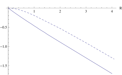
Figure 2: The temperature dependent part ${\cal F}_{T}$ of the free energy (in arbitrary units) of a scalar field for $\varepsilon=0$ and $T=1$ as function of $R$ calculated from the exact formula (solid line) and the corresponding proximity force approximation (dashed line).

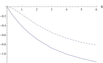
Figure 3: The temperature dependent part ${\cal F}_{T}$ of the free energy (in arbitrary units) of a scalar field for $\varepsilon=0.1$ and $T=1$ as function of $R$ calculated from the exact formula (solid line) and the corresponding proximity force approximation (dashed line).

Now we consider the region of medium and high temperature by keeping $d$ and $T$ fixed while $\varepsilon\to 0$. We start from representation 1 of the free energy for the electromagnetic field. We rewrite the Matsubara sum by inserting unity in the form

$$1=\int_{-\infty}^{\infty}d\xi\,\delta(\xi-\xi_{n}).$$ (64)

Interchanging the orders of summation and integration we come to the representation

$${\cal F}=\frac{T}{2}\int_{-\infty}^{\infty}d\xi\,\sum_{n=-\infty}^{\infty}\delta(\xi-\xi_{n})\ {\rm Tr}\ln\left(1-\mathbf{M}(\xi)\right).$$ (65)

Now we use the relation

$$\sum_{n=-\infty}^{\infty}\delta(\xi-\xi_{n})=\frac{1}{2\pi T}\sum_{n=-\infty}^{\infty}e^{in\xi/T},$$ (66)

which is equivalent to the Poisson resummation formula, and the free energy takes the form

$${\cal F}=\frac{1}{2}\int_{-\infty}^{\infty}\frac{d\xi}{2\pi}\,\sum_{n=-\infty}^{\infty}e^{in\xi/T}\ {\rm Tr}\ln\left(1-\mathbf{M}(\xi)\right).$$ (67)

This expression differs from the vacuum energy 2 only by the sum and the additional exponential factor. For this reason we can apply the same methods as in BORDAG2008C ; BORDAG2009C to calculate the asymptotic behavior for $\varepsilon\to 0$. First we expand the logarithm and come to a representation in parallel to 51,

$${\cal F}=-\frac{1}{2R}\int_{-\infty}^{\infty}\frac{d\xi}{2\pi}\,\sum_{n=-\infty}^{\infty}e^{in\xi/(RT)}\sum_{s=0}^{\infty}\frac{1}{s+1}\,\sum_{m=-\infty}^{\infty}\sum_{l=|m|}^{\infty}\left(\prod_{j=1}^{s}\sum_{n_{j}=|m|-l}^{\infty}\right){\cal Z}\left(\frac{\xi}{R}\right),$$ (68)

where ${\cal Z}$ is given by Eq.52. In 68, in addition we substituted $\xi\to\xi/R$. After that, $Z(\xi/R)$ is a function of $\varepsilon$ only. Now we consider the limit $\varepsilon\to 0$. For decreasing $\varepsilon$, the main contribution to the integral over $\xi$ and and to the sums over the orbital momenta come from higher and higher values. Therefore we substitute the orbital momentum sums by corresponding integrals and change the variables according to

$$\xi=\frac{t}{\varepsilon}\,\sqrt{1-\tau^{2}},\quad l=\frac{t}{\varepsilon}\,\tau,\quad m=\sqrt{\frac{t\tau}{\varepsilon}}\,\mu\,,$$

$$\quad n_{i}=\sqrt{\frac{4t}{\varepsilon}}\,\tilde{n}_{i}~{}~{}(i=1,\dots,s)\,.$$ (69)

In this way we get an asymptotic expansion in the form

$${\cal F} = -\frac{R}{4\pi d^{2}}\sum_{s=0}^{\infty}\frac{1}{s+1}\int_{0}^{\infty}dt\,t\ e^{-2t(s+1)}\int_{0}^{1}\frac{d\tau\,{\tau}}{\sqrt{1-\tau^{2}}}\,\sum_{n=-\infty}^{\infty}e^{int\sqrt{1-\tau^{2}}/(\varepsilon RT)}$$ (70)

$$\times\int_{-\infty}^{\infty}{d\mu}\ e^{-\mu^{2}(s+1)}\ \left(\prod_{j=1}^{s}\int_{-\infty}^{\infty}\frac{d\tilde{n}_{j}}{\sqrt{\pi}}\right)\cal{Z}^{\rm as}\,,$$

where

$${\cal Z}^{\rm as}=\prod_{i=0}^{s}\left(\sqrt{\frac{4\pi t}{\varepsilon}}\,M_{l+n_{i},l+n_{i+1}}\right)\,e^{2t(s+1)+\eta_{1}+\mu^{2}(s+1)}\,,$$ (71)

with $\eta_{1}=\sum_{i=0}^{s}(\tilde{n}_{i}-\tilde{n}_{i+1})^{2}$. We stress again that these formulas are in complete analogy to the corresponding ones in BORDAG2008C ; BORDAG2009C . The whole difference is in the sum over $n$ and the T-dependent exponential. For instance, the factor ${\cal Z}^{\rm as}$ is the same as without temperature. Therefore we know it has an expansion

$${\cal Z}^{\rm as}=1+O(\varepsilon).$$ (72)

The corrections $O(\varepsilon)$ depend only on the geometry and the kind of fields, but not on the temperature. Now we are interested in the pure temperature dependent contributions. Hence we drop these corrections and take ${\cal Z}^{\rm as}=1$. After that ${\cal F}$, Eq.70, can be simplified. First of all, one can perform the integrations over $\tilde{n}_{i}$ and $\mu$,

$${\cal F} = -\frac{R}{4\pi d^{2}}\sum_{s=0}^{\infty}\frac{1}{(s+1)^{2}}\int_{0}^{\infty}dt\,t\ e^{-2t(s+1)}\int_{0}^{1}\frac{d\tau\,{\tau}}{\sqrt{1-\tau^{2}}}\,\sum_{n=-\infty}^{\infty}e^{int\sqrt{1-\tau^{2}}/(\varepsilon RT)}.$$ (73)

Now the integration over $t$ is trivial. Also the integration over $\tau$ can be carried out leaving the double sum

$${\cal F} = -\frac{R}{4\pi d^{2}}\sum_{s=0}^{\infty}\frac{1}{(s+1)^{2}}\sum_{n=-\infty}^{\infty}\frac{\varepsilon^{2}T^{2}}{n^{2}+4\varepsilon^{2}(s+1)^{2}T^{2}}.$$ (74)

Here the contribution from $n=0$ is just the zero temperature contribution, i.e., the vacuum energy. For the remaining sum over $n\neq 0$ we use the formula

$$\sum_{n=1}^{\infty}\frac{1}{a^{2}+n^{2}}=\frac{a\pi\coth(a\pi)-1}{2a^{2}}$$ (75)

and the free energy can be written in the form

$${\cal F} = -\frac{R}{4\pi d^{2}}\left(1+h(2dT)\right),$$ (76)

where we defined

$$h(x)=90x^{4}\sum_{m=1}^{\infty}\left[\frac{\coth(m\pi x)}{(m\pi x)^{3}}-\frac{1}{(m\pi x)^{4}}\right].$$ (77)

In the last step we substituted $s+1\to m$.

In 76, the function $h(2dT)$ describes the temperature contribution to the free energy for medium and high temperature at small separation. It was derived from the exact formula 1. Now it is interesting to observe that this function, $h(x)$ as given by Eq.77, is just the same as the function $h(x)$, Eq.47, found in PFA in the preceding section. This can be shown, for example, by inserting the sum representation 25 for $g(x)$ into 47. For this it is useful to rewrite 25 in the form

$$g(x)=45x^{4}\sum_{m=1}^{\infty}\frac{1}{y}\frac{\partial}{\partial y}\left(-\frac{\coth(y)}{y}+\frac{1}{y^{2}}\right)_{\big{|}{y=m\pi x}}.$$ (78)

Obviously, the integration in 47 can be carried out explicitly and one comes just to Eq.77. In this way, we confirm the PFA 45 and with it all subsequent discussions in section 3.

A similar statement holds for the force. In taking the derivative with respect to the separation $d$ of 76, we have to consider the derivative of $h(x)/x^{2}$. For this derivative the following formula holds,

$$\frac{\partial}{\partial x}\frac{h(x)}{x}=-\frac{2}{x^{3}}\,g(x),$$ (79)

where $g(x)$ is the same function as in the temperature dependent part of the free energy for parallel plates 23. This can be seen directly by inserting 77 into the left side of 79 and comparing with 25. In this way, also Eq.39 for the force in PFA is shown to coincide with the exact expression obtained from the T-matrix representation 1.

Finally we mention that the function $h(x)$, like $g(x)$, Eq.26, has an inversion symmetry,

$$h\left(\frac{1}{x}\right)=\frac{5}{x^{2}}-\frac{h(x)}{x^{4}},$$ (80)

which can be derived from 26 and 79.

V The free energy at low temperature

In this section we consider the low temperature expansion of the free energy, i.e., we assume $T\ll 1/R$ and $T\ll 1/d$ not restricting the relation between $d$ and $R$. We start from representation 53. The lowest approximation for $T\to 0$ is, of course, the vacuum energy. The temperature corrections come from expanding ${\cal F}_{T}$, 54, for small $T$. In this section it is useful not to expand the logarithm and we take the representation

$${\cal F}_{T}=\frac{1}{2\pi}\int_{0}^{\infty}{d\xi}\ n_{T}(\xi)\,i\,{\rm Tr}\left[\ln(1-\mathbf{M}(i\xi))-\ln(1-\mathbf{M}(-i\xi))\right].$$ (81)

For $T\to 0$, because of the Boltzmann factor, we can expand the remaining part of the integrand in 81 in powers of $\xi$. Each additional power in $\xi$ will add a power in $T$. So we need the lowest odd power of $\xi$. The lowest even power of $\xi$ does not contribute to the difference between the logarithms which in fact represent the jump across the cut the logarithm has.

First we expand $M_{l,l^{\prime}}(\xi)$, 3. We use the ascending series of the modified Bessel functions (see, for example AbramowitzStegun ),

$$I_{\nu}(z)=\left(\frac{z}{2}\right)^{\nu}\frac{i_{\nu}}{\Gamma(\nu+1)},\qquad K_{\nu}(z)=(-1)^{l}\,\frac{\pi}{2}\left(\frac{z}{2}\right)^{-\nu}\left(\frac{i_{-\nu}}{\Gamma(1-\nu)}-\left(\frac{z}{2}\right)^{2l+1}\frac{i_{\nu}}{\Gamma(1+\nu)}\right),$$ (82)

where $i_{\nu}$ has only even powers of $z$ and we continue to use the convention $\nu\equiv l+1/2$. Inserting these expansions into 3 and remembering that only $l^{\prime\prime}$ give non-zero contributions for which $l+l^{\prime}-l^{\prime\prime}$ is even, we observe that the first odd power of $\xi$ comes from the second term in $K_{\nu}(z)$ in 82. Moreover, the lowest odd power comes from the lowest orbital momenta $l$ and $l^{\prime}$ only. For this reason from the orbital momentum sums only one term remains and the logarithm can be calculated directly. For Dirichlet resp. Neumann boundary conditions on the sphere we obtain in this way for the scalar field

$$M_{0,0}^{\rm D}(\xi) = \frac{R}{2L}-\left(1-\frac{R}{2L}\right)R\xi+\dots\,,$$

$$M_{0,0}^{\rm N}(\xi) = -\frac{R^{3}}{6L}\xi^{2}+\frac{1}{3}R^{3}\xi^{3}+\dots\,.$$ (83)

The logarithms are

$$\ln\left(1-M_{0,0}^{\rm D}(\xi)\right) = \ln\left(1-\frac{R}{2L}\right)+R\xi+\dots$$

$$\ln\left(1-M_{0,0}^{\rm N}(\xi)\right) = \frac{R^{3}}{6L}\xi^{2}-\frac{1}{3}R^{3}\xi^{3}+\dots$$ (84)

and the jumps become

$$i\,{\rm Tr}\left[\ln(1-\mathbf{M^{\rm D}}(i\xi))-\ln(1-\mathbf{M^{\rm D}}(-i\xi))\right]=-2R\xi+\dots\,,$$

$$i\,{\rm Tr}\left[\ln(1-\mathbf{M^{\rm N}}(i\xi))-\ln(1-\mathbf{M^{\rm N}}(-i\xi))\right]=-\frac{2}{3}R^{3}\xi^{3}+\dots\,.$$ (85)

Finally we have to insert this into 81. The remaining integration can be done in terms of zeta functions and we come to

$${\cal F}_{T}^{\rm D} = -\frac{\zeta(2)}{\pi}\,RT^{2}+\dots\,,$$

$${\cal F}_{T}^{\rm N} = -\frac{2\zeta(4)}{\pi}\,R^{3}T^{4}+\dots\,.$$ (86)

These formulas are for Dirichlet boundary conditions on the plane. For Neumann boundary conditions on the plane we have to reverse the sign in the logarithms in 81. A simple calculation in parallel to the above one results in

$${\cal F}_{T}^{\rm D} = \frac{\zeta(2)}{\pi}\frac{2L-R}{2L+R}\,RT^{2}+\dots\,,$$

$${\cal F}_{T}^{\rm N} = \frac{2\zeta(4)}{\pi}\,R^{3}T^{4}+\dots\,.$$ (87)

We see that the leading order in the low temperature expansion follows the behavior for low momentum of the corresponding T-matrix. For Dirichlet boundary conditions, from the s-wave, the lowest order is $\xi$ resulting in correction of order $T^{2}$. For Neumann boundary conditions, due to the derivatives, this contribution is absent and the expansion starts with $T^{4}$.

For the electromagnetic field we have to take care of the polarizations. However, the off-diagonal entries of the matrix $\mathbf{M}$ start with an additional power in $\xi$ resulting from $\tilde{\Lambda}$. Since these enter the trace in quadratic combinations only, an additional power of $\xi^{2}$ as compared to the diagonal contributions results. As a consequence, the off-diagonal entries do not contribute to the leading order at small $T$. So we are left with, separately, the contributions from the TE and TM modes. For these, the same considerations as for the scalar field apply with the only difference of 19 in place of 4 and the orbital momentum sum starting from the p-wave. We write down explicitly the relevant contributions to $M_{l,l^{\prime}}(\xi)$ for both modes and for relevant values of the azimuthal index $m$,

$$M_{1,1}^{{\rm TE},m=0}(\xi) = \frac{R^{3}}{8L^{3}}-\frac{R^{3}}{4L}\left(1-\frac{3R^{2}}{10L^{2}}\right)\xi^{2}+\frac{R^{3}}{3}\left(1-\frac{R^{3}}{8L^{3}}\right)\xi^{3}+\dots\,,$$

$$M_{1,1}^{{\rm TE},m=1}(\xi) = \frac{R^{3}}{16L^{3}}+\frac{R^{3}}{8L}\left(1+\frac{3R^{2}}{10L^{2}}\right)\xi^{2}-\frac{R^{3}}{3}\left(1+\frac{R^{3}}{16L^{3}}\right)\xi^{3}+\dots\,,$$

$$M_{1,1}^{{\rm TM},m=0}(\xi) = \frac{R^{3}}{4L^{3}}-\frac{R^{3}}{2L}\left(1+\frac{3R^{2}}{20L^{2}}\right)\xi^{2}+\frac{2R^{3}}{3}\left(1+\frac{R^{3}}{4L^{3}}\right)\xi^{3}+\dots\,,$$

$$M_{1,1}^{{\rm TM},m=1}(\xi) = \frac{R^{3}}{8L^{3}}+\frac{R^{3}}{4L}\left(1-\frac{3R^{2}}{20L^{2}}\right)\xi^{2}-\frac{2R^{3}}{3}\left(1-\frac{R^{3}}{8L^{3}}\right)\xi^{3}+\dots\,.$$ (88)

From here we calculate the jumps just like in V. Introducing the symbolic notation $\Delta$ for these we note

$$\Delta^{{\rm TE},m=0} = -\frac{2}{3}\,R^{3}\xi^{3}+\dots\,,$$

$$\Delta^{{\rm TE},m=1} = \frac{2}{3}\frac{16L^{3}+R^{3}}{16L^{3}-R^{3}}\,R^{3}\xi^{3}+\dots\,,$$

$$\Delta^{{\rm TM},m=0} = -\frac{4}{3}\frac{4L^{3}+R^{3}}{4L^{3}-R^{3}}\,R^{3}\xi^{3}+\dots\,,$$

$$\Delta^{{\rm TM},m=1} = \frac{4}{3}\,R^{3}\xi^{3}+\dots\,.$$ (89)

These expressions we have to insert into ${\cal F}_{T}$ and to integrate over $\xi$. In the end we get

$${\cal F}_{T}=\frac{6\zeta(4)}{\pi}\left(1+\frac{2}{3}\frac{16L^{3}+R^{3}}{16L^{3}-R^{3}}-\frac{2}{3}\frac{4L^{3}+R^{3}}{4L^{3}-R^{3}}\right)\,R^{3}T^{4}+\dots\,.$$ (90)

This is the low temperature correction for the electromagnetic field. We see that it gives an order $T^{4}$ contribution like for the forces acting between parallel plates.

Now we can consider 90 for small separation. We can put $d=0$ directly and get

$${\cal F}_{T}=\frac{58\zeta(4)}{15\pi}\,R^{3}T^{4}+\dots\,.$$ (91)

This expression is, as expected, different from the temperature corrections in PFA, Eq.40. It gives the low temperature (this is $T\ll 1/R$) correction beyond PFA.

It is also possible to consider 90 for large separation, or equivalently, for small $R$. One gets

$${\cal F}_{T}=\frac{6\zeta(4)}{\pi}\left(1-\frac{R^{3}}{4d^{3}}+\dots\right)\,R^{3}T^{4}\,.$$ (92)

The leading order coincides with the corresponding low temperature expansion of Eq.(4) in Durand2009 .

VI The free energy at high temperature

The high temperature expansion can best be analyzed starting from the original Matsubara sum 1. The leading order for $T\to\infty$ is given by the contribution with $n=0$, i.e., by the lowest Matsubara frequency.

We separate the contribution from $n=0$,

$${\cal F}=TF_{0}\left(\frac{d}{R}\right)+F_{1}(Td,TR)$$ (93)

and the contributions with $n\neq 0$ are collected in $F_{1}$. The leading contribution $F_{0}$ is proportional to $T$ and it is a function of the dimensionless ratio 21. The function $F_{1}$ depends on two dimensionless combinations.

We consider the function $F_{0}$ in more detail. It is given by the formula

$$F_{0}(\varepsilon)=\frac{1}{2}\,{\rm Tr}\ln(1-\mathbf{M}(0)).$$ (94)

From 3 and using 82 we get for the scalar field with Dirichlet boundary conditions on the sphere

$$M_{l,l^{\prime}}^{\rm D}(0)=\left(\frac{R}{2L}\right)^{l+l^{\prime}+1}\frac{\sqrt{\pi}\,\Gamma(l+l^{\prime}+1/2)}{2\Gamma(l+1/2)\Gamma(l^{\prime}+3/2)}\,H_{l,l^{\prime}}^{l+l^{\prime}}.$$ (95)

Here we took into account that from the sum over $l^{\prime\prime}$ in 3 only the term with $l^{\prime\prime}=l+l^{\prime}$ did contribute. For Neumann boundary condition on the sphere we have to account for the derivatives. These result in a simple factor and we can write

$$M_{l,l^{\prime}}^{\rm N}(0)=\frac{-l^{\prime}}{l+1}\,M_{l,l^{\prime}}^{\rm D}(0)$$ (96)

For the electromagnetic field we have in addition the terms mixing the polarizations. However, since $\tilde{\Lambda}_{l,l^{\prime}}$ is proportional to $\xi$ these do not contribute. So we are left with the additional factor $\Lambda_{l,l^{\prime}}^{l^{\prime\prime}}$ and the difference in the derivatives. We come to

$$M_{l,l^{\prime}}^{\rm TE}(0)=M_{l,l^{\prime}}^{\rm D}(0)\,\Lambda_{l,l^{\prime}}^{l+l^{\prime}},\qquad M_{l,l^{\prime}}^{\rm TM}(0)=\frac{l^{\prime}+1}{l}\,M_{l,l^{\prime}}^{\rm D}(0)\,\Lambda_{l,l^{\prime}}^{l+l^{\prime}}.$$ (97)

These expressions can be inserted into 94 and for any finite $\varepsilon=d/R\neq 0$ the function $F_{0}$ can be calculated numerically.

We consider the limiting cases of $\varepsilon\to\infty$ (large separation) and $\varepsilon\to 0$ (small separation). For large separation we simply have to expand the $M_{l,l^{\prime}}(0)$ into powers of $1/\varepsilon$ and see that only the lowest orbital momenta contribute. We obtain

$$M_{0,0}^{\rm D}(0)=\frac{R}{2L}+\dots, M_{0,0}^{\rm N}(0)=-2\left(\frac{R}{2L}\right)^{3}+\dots,$$

$$M_{1,1^{\prime}}^{\rm TE}(0)=2\left(\frac{R}{2L}\right)^{3}+\dots, M_{1,1}^{\rm TM}(0)=4\left(\frac{R}{2L}\right)^{3}+\dots\,.$$ (98)

The corresponding functions $F_{0}$ we get from 94 in this approximation by multiplication with $(-1/2)$. For the electromagnetic field, i.e., adding the two contributions in the lower line in VI, the result coincides with the lower line in Eq.(6) in Durand2009 .

In the opposite limit of small separation, i.e., for $\varepsilon\to 0$ we are faced with the problem that the convergence of the orbital momentum sums gets lost. This problem is essentially the same as at zero temperature in the same limit. Even more, it can be treated by the same methods, i.e., by calculating the asymptotic expansion of $F_{0}(\varepsilon)$ for $\varepsilon\to 0$. The first step in this procedure is to expand the logarithm in 94 and to substitute the orbital momentum sums by corresponding integrations,

$$F_{0}(\varepsilon)=-\sum_{s=0}^{\infty}\frac{1}{s+1}\int_{0}^{\infty}dl\,\int_{-l}^{l}dm\,\left(\prod_{j=1}^{s}\int_{l-m}^{\infty}dn_{j}\right){\cal Z}$$ (99)

with

$${\cal Z}=\prod_{i=0}^{s}M_{l+n_{i},l+n_{i+1}}(0)\,.$$ (100)

We mention that this is, up to the sums substituted by integrals, the $(n=0)$-contribution in 51. Next we have to make an appropriate substitution of variables,

$$l=\frac{t}{\varepsilon},\quad m=\sqrt{\frac{t}{\varepsilon}}\,\mu,\quad n_{i}=\sqrt{\frac{4t}{\varepsilon}}\,\tilde{n}_{i}\,.$$ (101)

This is the same substitution as used in BORDAG2008C , Eq.(8) and in BORDAG2009C , Eq.(28), here however restricted to $\tau=1$. Therefore we can use the asymptotic formulas derived there. For instance, in leading order we have

$$M_{l+n,l+n^{\prime}}(0)=\left(\frac{\varepsilon}{4\pi t}\right)^{1/2}\ e^{-2t-(n-n^{\prime})^{2}-\mu^{2}}(1+O(\varepsilon)).$$ (102)

This expression is the same for both boundary conditions and also for the modes of the electromagnetic field. For the latter there is in this approximation also no mixing of the polarizations, for details see BORDAG2009C . Making in 99 the substitution 101 we come for the electromagnetic field with 102 to

$$F_{0}(\varepsilon)=-\frac{1}{2\varepsilon}\sum_{s=0}^{\infty}\frac{1}{s+1}\int_{0}^{\infty}dt\,e^{-2t(s+1)}\int_{-\infty}^{\infty}\frac{d\mu}{\sqrt{\pi}}\ e^{-\mu^{2}(s+1)}\left(\prod_{j=1}^{s}\int_{-\infty}^{\infty}\frac{d\tilde{n}_{j}}{\sqrt{\pi}}\right)e^{-\eta_{1}}+\dots$$ (103)

with $\eta_{1}=\sum_{i=0}^{s}(\tilde{n}_{i}-\tilde{n}_{i+1})^{2}.$ Carrying out the integrations and the sum we obtain

$$F_{0}(\varepsilon)=-\frac{\zeta(3)}{4\varepsilon}+\dots$$ (104)

We mention that this formula coincides with the corresponding PFA result 49 although we did not assume $d\ll R$.

In general, the contribution of the zeroth Matsubara frequency is equivalent to a theory with a dimension reduced by one. However, thereby it is usually assumed that the original theory (taken in its Euclidean version) has a symmetry between the spatial and the time dimensions. One must bear in mind that in the given case this symmetry is broken by the boundaries.

Finally we consider $F_{1}$ in 93, i.e., the contributions from the non-zero Matsubara frequencies. Here we observe for large $T$ an exponential decrease of the functions $M_{l,l^{\prime}}(0)$,

$$M_{l,l^{\prime}}(0)\sim e^{-4\pi nTd}$$ (105)

($d=L-R$) such that $F_{1}$ is exponentially suppressed for all $d>0$. This is the same property as we observe in the case of parallel planes. This suppression holds for for $\frac{1}{T}\ll d$, $\frac{1}{T}\ll R$. If in addition $d\ll R$, i.e. $\frac{1}{T}\ll d\ll R$, holds this suppression disappears. In that case, as before, higher and higher $n$ and orbital momenta contribute. In fact, this is the limit $RT\to\infty$ in the region of high temperature as defined in section 3, Eq.20. In that case it is appropriate use representation 67 and to proceed as it was done in the second part of section 4. As a result, $F_{1}$ would deliver a correction beyond what is displayed in Eq.76.

VII Conclusions

In the foregoing sections we calculated the free energy for a sphere in front of a plane at finite temperature for conductor boundary conditions. First we considered the case of small separation. Here we used both methods, the PFA and the functional determinant representation and considered both, the free energy and the force. In the region of low temperature, the thermal contributions to the free energy and to the force are very small and PFA does not hold for them. In the region of medium and high temperatures, which is the temperature region of experimental interest, we have reproduced the PFA from the exact method. For instance we have shown that the rule 34 does hold in this case.

We would like to mention that in Milton:2009gk exact finite temperature results were obtained for the interaction between a plane and a semitransparent curved surface described by a delta-potential. For weak coupling it was shown that the free energy of a scalar field coincides at all temperatures with the proximity force approximation corresponding to this geometry.

Next we considered low temperature without restriction to small separation and derived the corresponding expansions for the free energy. Here the behavior of the thermal contribution to the free energy depends on the boundary conditions and on the kind of the field. An interesting question on the interplay between temperature and geometry was raised in Weber:2009dp ; Gies:2009nn . There it was observed that in an open geometry at low temperature lower powers of the temperature may appear as compared with the parallel planes. In general, we cannot support this conclusion from our calculations. Only for a scalar field with Dirichlet boundary conditions we observe ${\cal F}_{T}\sim T^{2}$, Eq.V. For Neumann boundary conditions and for the electromagnetic field we see ${\cal F}_{T}\sim T^{4}$, Eqs.V (lower line), V and 91.

In section 6 we considered the limit of high temperature. As expected, here the dimensional reduction works and the leading order contribution comes from the zeroth Matsubara frequency. At small separation, the asymptotics could be calculated using the same methods as for zero temperature and the result coincides with that of PFA.

This work was supported by the Heisenberg-Landau program. The authors acknowledge helpful discussions with G.Klimchitskaya and V.Mostepanenko. The authors benefited from exchange of ideas by the ESF Research Network CASIMIR.

References

- [1] Alexej Weber and Holger Gies. Interplay between geometry and temperature for inclined Casimir plates. Phys. Rev., D80:065033, 2009.
- [2] Holger Gies and Alexej Weber. Geometry-Temperature Interplay in the Casimir Effect. 2009. arXiv:0912.0125.
- [3] Antoine Canaguier-Durand, Paulo A. Maia Neto, Astrid Lambrecht, and Serge Reynaud. Thermal casimir effect in the sphere-plane geometry. Phys.Rev.Lett, 104:040403, 2010.
- [4] Aurel Bulgac, Piotr Magierski, and Andreas Wirzba. Scalar Casimir effect between Dirichlet spheres or a plate and a sphere. Phys. Rev., D73:025007, 2006.
- [5] T. Emig, N. Graham, R. L. Jaffe, and M. Kardar. Casimir forces between arbitrary compact objects. Phys. Rev. Lett., 99:170403, 2007.
- [6] M. Bordag and V. Nikolaev. Casimir force for a sphere in front of a plane beyond proximity force approximation. J. Phys. A: Math. Gen., 41:164001, 2008.
- [7] M. Bordag, G.L. Klimchitskaya, U. Mohideen, and V.M. Mostepanenko. Advances in the Casimir Effect. Oxford University Press, 2009.
- [8] M. Bordag and V. Nikolaev. First analytic correction beyond PFA for the electromagnetic field in sphere-plane geometry. Phys.Rev.D, in press, 2010. ArXiv: 0911.0146.
- [9] M. Bordag, U. Mohideen, and V. M. Mostepanenko. New developments in the Casimir effect. Phys. Rep., 353:1–205, 2001.
- [10] J. Blocki, J. Randrup, W. J. Swiatecki, and C. F. Tsang. Proximity forces. Annals Phys., 105:427–462, 1977.
- [11] M. Bordag. The Casimir effect for a sphere and a cylinder in front of plane and corrections to the proximity force theorem. Phys. Rev., D73:125018, 2006.
- [12] M. Abramowitz and I.A. Stegun. Handbook of mathematical functions: with formulas, graphs, and mathematical tables. Dover, New York, 1972.
- [13] Kimball A. Milton, Prachi Parashar, Jef Wagner, and K. V. Shajesh. Exact Casimir energies at nonzero temperature: Validity of proximity force approximation and interaction of semitransparent spheres. 2009. arXiv: 0909.0977.