Abundance analysis of a sample of evolved stars in the outskirts of $\omega$ Centauri

Abstract

The globular cluster $\omega$ Centauri (NGC 5139) is a puzzling stellar system harboring several distinct stellar populations whose origin still represents a unique astrophysical challenge. Current scenarios range from primordial chemical inhomogeneities in the mother cloud to merging of different sub-units and/or subsequent generations of enriched stars - with a variety of different pollution sources- within the same potential well. In this paper we study the chemical abundance pattern in the outskirts of $\omega$  Centauri, half-way to the tidal radius (covering the range of 20-30 arcmin from the cluster center), and compare it with chemical trends in the inner cluster regions, in an attempt to explore whether the same population mix and chemical compositions trends routinely found in the more central regions is also present in the cluster periphery. We extract abundances of many elements from FLAMES/UVES spectra of 48 RGB stars using the equivalent width method and then analyze the metallicity distribution function and abundance ratios of the observed stars. We find, within the uncertainties of small number statistics and slightly different evolutionary phases, that the population mix in the outer regions cannot be distinguished from the more central regions, although it is clear that more data are necessary to obtain a firmer description of the situation. From the abundance analysis, we did not find obvious radial gradients in any of the measured elements.

1 Introduction

Multiple stellar populations are routinely found in old Galactic and intermediate-age Magellanic Clouds star clusters (Piotto 2008 and references therein). Whether they are a signature of the cluster formation process or a result of the star formation history and related stellar evolution effects, is still matter of lively discussion (Renzini 2008, Bekki et al. 2008, Decressin et al. 2007). The prototype of globular hosting multiple populations has for long time been $\omega$  Cen (Villanova et al. 2007), although the current understanding is that it is possibly the remnant of a dwarf galaxy (Carraro & Lia 2000, Tsuchiya et al. 2004, Romano et al. 2007).
Most chemical studies of the stellar population in $\omega$  Cen are restricted within 20 arcmin of the cluster radius center (see Norris & Da Costa 1995, Villanova et al. 2007), where, probably, the diverse stellar components are better mixed and less subjected to external perturbations, like the Galactic tidal stress, than the outer regions. Assessing whether there are population inhomogeneities in $\omega$ Cen or gradients in metal abundance is a crucial step to progress in our understanding of this fascinating stellar system.
In Scarpa et al. (2003, 2007) we presented the results of a spectroscopic campaign to study the stellar radial velocity dispersion profile at $\sim$ 25 arcmin, half way to the tidal radius ($\sim$ 57 arcmin, Harris 1996), in an attempt to find a new way to verify the MOND (Modified Newtonian Dynamics, Milgrom 1983) theory of gravitation.
In this paper we make use of a subsample of those spectra (the ones taken for RGB stars) and extract estimates of metal abundances for some of the most interesting elements. The aim is to study the chemical trends of the stellar populations in the cluster periphery, to try to learn whether the cluster outskirts contain, both qualitatively and quantitatively, the same population mix and to infer from this additional information on the cluster formation and evolution.
The layout of the paper is as follows. In Sect. 2 we describe observations and data reduction, while Sect. 3 is dedicated to the derivation of metal abundances. These latter are then discussed in detail in Sect. 4. Sect. 5 is devoted to the comparison of the metal abundance trends in the inner and outer regions of $\omega$  Cen, and, finally, Sect. 6 summarizes the findings of this study.

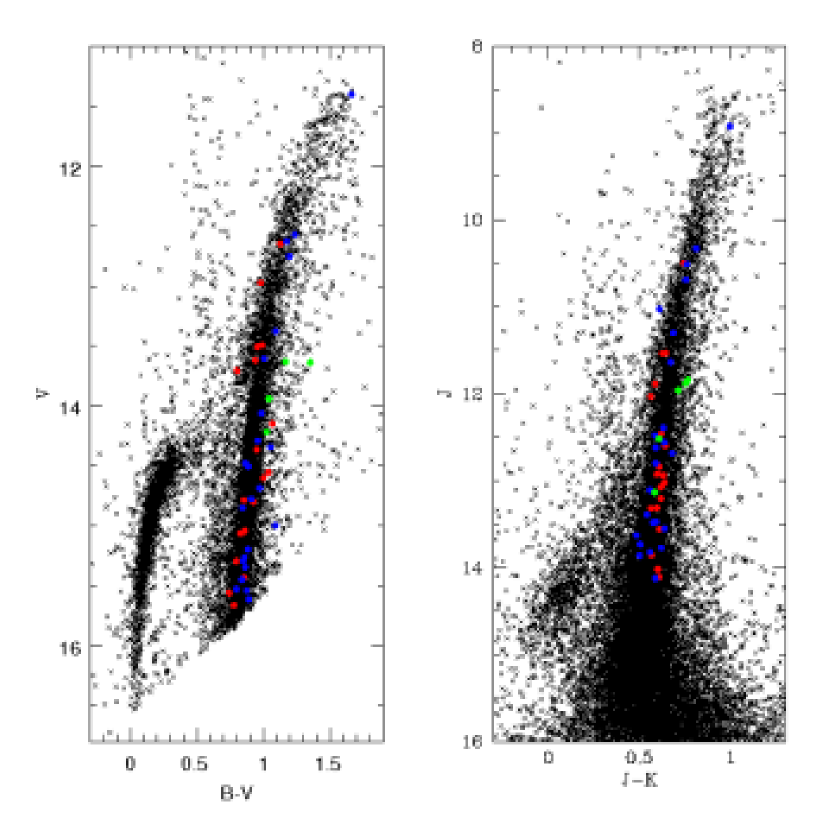
Figure 1: The CMD of $\omega$  Cen in the optical (left panel) and infrared. Solid symbols of different colors indicate stars belonging to the MPP (red), IMP (blue) and MRP(green). See text for more details.

Figure 2: Distribution of iron abundance for the program stars. A bimodal Gaussian fit is used to derive the mean iron abundance of the MPP and IMP. Mean iron abundances of the three peaks are indicated. See text for more details.

Table 1: Measured Solar abundances ($\rm{log\epsilon(X)=log(N_{X}/N_{H})+12)}$.

Element	log$\epsilon$(X)
NaI	6.37
MgI	7.54
SiI	7.61
CaI	6.39
TiI	4.94
TiI	4.96
CrI	5.63
FeI	7.50
NiI	6.28
ZnI	4.61
YII	2.25
BaI	2.31

2 Observations and Data reduction

Our data-set consists of UVES spectra collected in August 2001, for a project devoted to measuring radial velocities and establishing membership in the outskirts of the cluster. Data were obtained with UVES/VLT@UT2 (Pasquini et al. 2002) with a typical seeing of 0.8-1.2 arcsec. We observed isolated stars from the lower red giant branch (RGB) up to the tip of the RGB of $\omega$ Cen, in the magnitude range $11.5<{\rm V}<16.0$.

We used the UVES spectrograph in the RED 580 setting. The spectra have a spectral coverage of $\sim$2000 Å with the central wavelength at 5800 Å. The typical signal to noise ratio is ${\rm S/N\sim 20-30}$. For additional details, the reader is referred to Scarpa et al. (2003).

Data were reduced using UVES pipelines (Ballester et al. 2000), including bias subtraction, flat-field correction, wavelength calibration, sky subtraction and spectral rectification. Stars were selected from photographic BV observations (van Leeuwen et al. 2000) coupled with infrared JHK 2MASS photometry (Skrutskie et al. 2006). Targets are located at a radial distance between 20 and 30 arcmin. The whole sample of stars contain both RGB and horizontal branch (HB) stars. In this paper we focus our attention only on RGB objects, for the sake of comparison with previous studies.

2.1 Radial velocities and membership

In the present work, radial velocities were used as the membership criterion since the cluster stars all have similar motions with respect to the observer. The radial velocities of the stars were measured using the IRAF FXCOR task, which cross-correlates the object spectrum with a template. As a template, we used a synthetic spectrum obtained through the spectral synthesis code SPECTRUM (see http://www.phys.appstate.edu/spectrum/spectrum.html for more details), using a Kurucz model atmosphere with roughly the mean atmospheric parameters of our stars $\rm{T_{eff}=4900}$ K, $\rm{log(g)=2.0}$, $\rm{v_{t}=1.3}$ km/s, $\rm{[Fe/H]=-1.40}$. Each radial velocity was corrected to the heliocentric system. We calculated a first approximation mean velocity and the r.m.s ($\sigma$) of the velocity distribution. Stars showing $\rm{v_{r}}$ out of more than $3\sigma$ from the mean value were considered probable field objects and rejected, leaving us with 48 UVES spectra of probable members, whose position in the CMD are shown in Fig. 1. Radial velocities for member stars are reported in Tab. 2

3 Abundance analysis

3.1 Continuum determination

The chemical abundances for all elements were obtained from the equivalent widths (EWs) of the spectral lines (see next Section for the description of the line-list we used). An accurate measurement of EWs first requires a good determination of the continuum level. Our relatively metal-poor stars allowed us to proceed in the following way. First, for each line, we selected a region of 20 Å centered on the line itself (this value is a good compromise between having enough points, i. e. a good statistic, and avoiding a too large region where the spectrum might not be flat). Then we built the histogram of the distribution of the flux where the peak is a rough estimation of the continuum. We refined this determination by fitting a parabolic curve to the peak and using the vertex as our continuum estimation. Finally, we revised the continuum determination by eye and corrected by hand if an obvious discrepancy with the spectrum was found. Then, using the continuum value previously obtained, we fit a Gaussian curve to each spectral line and obtained the EW from integration. We rejected lines if they were affected by bad continuum determinations, by non-Gaussian shape, if their central wavelength did not agree with that expected from our line-list, or if the lines were too broad or too narrow with respect to the mean FWHM. We verified that the Gaussian shape is a good approximation for our spectral lines, so no Lorenzian correction has been applied.

Table 2: Stellar parameters. Coordinates are for J2000.0 equinox

ID	$\alpha$	$\delta$	B	V	J2MASS	H2MASS	K2MASS	Teff	log(g)	vt	RVH
	deg	deg.						${}^{0}K$		km/sec	km/sec
00006	201.27504	-47.15599	16.327	15.531	13.865	13.386	13.364	5277	2.75	1.23	222.99
08004	201.07113	-47.22082	15.393	14.508	12.687	12.110	12.007	4900	2.17	1.38	241.70
10006	201.16314	-47.23357	14.510	13.710	11.887	11.413	11.300	5080	1.93	1.44	237.18
10009	201.24457	-47.23406	13.807	12.573	10.331	9.664	9.520	4432	1.14	1.64	227.57
10010	201.33458	-47.23334	14.982	13.941	11.963	11.394	11.249	4758	1.88	1.45	220.18
13006	201.13373	-47.25880	16.442	15.665	14.112	13.615	13.504	5251	2.79	1.22	231.78
14002	201.16243	-47.26471	15.696	14.853	13.110	12.634	12.552	5151	2.42	1.31	224.00
22007	201.08521	-47.32639	14.799	13.635	11.843	11.221	11.077	4750	1.75	1.49	227.25
25004	201.18696	-47.34607	15.048	14.064	12.393	11.852	11.762	5034	2.06	1.41	230.68
27008	201.16507	-47.36326	15.242	14.220	12.519	12.046	11.911	5095	2.15	1.38	237.50
28009	201.13729	-47.36499	15.687	14.779	13.133	12.664	12.549	5186	2.41	1.32	236.00
33006	201.12822	-47.40730	13.062	11.403	8.924	8.064	7.929	4051	0.39	1.83	226.34
34008	201.19496	-47.41343	13.803	12.629	10.510	9.897	9.749	4570	1.25	1.61	232.16
38006	201.11643	-47.44354	16.289	15.436	13.822	13.304	13.263	5202	2.68	1.25	222.58
39013	201.16078	-47.45089	13.950	12.755	10.690	10.097	9.935	4610	1.32	1.59	231.47
42012	201.17440	-47.47487	14.468	13.379	11.299	10.705	10.613	4673	1.61	1.52	232.58
43002	201.14213	-47.47916	15.313	14.365	12.597	12.113	11.956	5021	2.17	1.38	229.17
45011	201.10941	-47.49389	16.208	15.346	13.630	13.146	13.146	5229	2.66	1.25	224.37
45014	201.15625	-47.50013	15.894	15.066	13.316	12.803	12.720	5073	2.47	1.30	249.24
46003	201.12943	-47.50252	15.640	14.788	13.073	12.578	12.455	5091	2.37	1.33	242.00
48009	201.12036	-47.51844	16.504	15.616	14.125	13.602	13.537	5279	2.79	1.22	222.94
49008	201.16235	-47.52717	15.657	14.687	12.799	12.256	12.210	4925	2.26	1.36	238.57
51005	201.09190	-47.53945	16.140	15.292	13.551	13.005	12.913	5028	2.55	1.28	221.27
57006	201.18559	-47.58523	15.906	15.046	13.320	12.797	12.757	5096	2.48	1.30	234.33
61009	201.16032	-47.61620	14.488	13.496	11.533	10.947	10.890	4784	1.71	1.50	239.65
76015	201.33839	-47.73435	15.602	14.604	12.839	12.355	12.231	5026	2.27	1.35	241.73
77010	201.23548	-47.74124	14.992	13.641	11.886	11.269	11.133	4746	1.75	1.49	238.49
78008	201.21908	-47.74676	16.088	15.001	13.484	12.990	12.909	5221	2.52	1.29	223.14
80017	201.40179	-47.75878	15.250	14.294	12.481	11.989	11.896	5026	2.15	1.38	231.59
82012	201.44193	-47.77921	16.094	15.298	13.558	13.059	12.947	5099	2.58	1.27	232.28
85007	201.19307	-47.80062	-	-	14.020	13.489	13.419	4983	2.20	1.37	250.48
85014	201.37723	-47.80134	15.400	14.347	12.560	11.982	11.923	4899	2.11	1.39	236.78
85019	201.53965	-47.80194	15.727	14.803	12.939	12.428	12.308	4938	2.31	1.34	243.81
86007	201.22490	-47.80442	-	-	13.024	12.487	12.387	4914	1.88	1.45	238.70
86010	201.31217	-47.80789	15.594	14.557	12.926	12.437	12.329	5115	2.29	1.35	238.05
86017	201.56208	-47.80760	16.289	15.452	13.737	13.319	13.232	5290	2.73	1.24	231.74
87009	201.61710	-47.81630	16.081	15.199	13.392	12.885	12.850	5082	2.54	1.29	247.67
88023	201.58521	-47.82029	16.415	15.542	13.774	13.268	13.154	5050	2.66	1.25	232.87
89009	201.57067	-47.83291	13.776	12.650	10.497	9.890	9.753	4568	1.25	1.61	242.07
89014	201.66544	-47.83110	14.611	13.607	11.639	11.055	10.967	4774	1.75	1.49	231.57
90008	201.22516	-47.83980	-	-	13.209	12.703	12.591	5010	1.95	1.43	240.42
90019	201.62529	-47.83825	14.462	13.509	11.537	11.018	10.911	4860	1.75	1.48	232.73
90020	201.64363	-47.83814	16.305	15.563	13.858	13.395	13.292	5219	2.74	1.23	240.39
93016	201.65058	-47.86211	15.342	14.479	12.620	12.107	12.031	5015	2.22	1.37	230.82
94011	201.30980	-47.86480	15.217	14.151	12.462	11.911	11.842	4989	2.07	1.40	241.74
95015	201.54907	-47.87303	16.122	15.264	13.475	12.977	12.884	5076	2.56	1.28	239.10
96011	201.52316	-47.88203	13.954	12.975	11.027	10.514	10.416	4894	1.56	1.53	229.55
98012	201.35549	-47.89600	14.561	13.623	12.034	11.552	11.471	5210	1.96	1.43	229.93

Table 3: Stellar abundances

ID	FeI	${\rm[FeI/H]}$	NaI	MgI	SiI	CaI	TiI	TiII	CrI	NiI	ZnI	YII	BaII
00006	6.15	-1.35	4.91	6.27	6.63	5.25	3.94	3.89	4.11	4.61	3.35	1.06	1.27
08004	6.23	-1.27	5.74	6.31	6.97	5.53	4.12	4.30	4.38	5.01	3.61	1.75	1.93
10006	5.80	-1.70	-	-	-	5.03	3.77	3.64	3.76	-	3.09	-	1.57
10009	6.18	-1.32	5.61	6.38	-	5.27	3.93	4.03	4.24	5.04	3.04	1.26	1.69
10010	6.45	-1.05	5.38	6.71	-	5.65	3.91	4.02	4.65	5.07	3.42	1.86	2.08
13006	5.93	-1.57	-	6.31	-	5.06	3.88	3.61	4.04	-	2.95	-	0.37
14002	6.02	-1.48	-	-	-	5.25	3.90	3.72	4.00	5.19	3.28	0.61	1.15
22007	6.43	-1.07	5.80	6.88	6.85	5.61	4.07	4.17	4.51	5.09	3.54	1.80	2.00
25004	6.14	-1.36	-	-	-	5.44	4.09	3.81	3.95	-	-	-	1.08
27008	6.52	-0.98	-	-	7.29	5.60	4.30	4.24	4.91	-	-	1.86	2.71
28009	6.29	-1.21	-	-	-	5.53	4.20	4.29	-	4.97	-	-	0.65
33006	6.07	-1.43	-	6.38	-	5.30	4.10	4.27	4.32	4.73	-	-	1.43
34008	6.11	-1.39	5.52	6.24	-	5.29	3.87	3.99	4.00	4.83	-	1.27	1.54
38006	5.97	-1.53	-	6.19	-	5.15	3.79	3.88	4.16	4.99	3.19	0.65	0.61
39013	6.01	-1.49	-	6.51	6.85	5.30	3.77	3.71	4.13	4.80	-	1.34	1.17
42012	6.10	-1.40	5.05	6.62	6.66	5.42	3.93	4.08	4.22	4.85	3.37	1.62	1.61
43002	5.94	-1.56	5.10	6.09	-	5.24	3.96	3.81	4.29	-	-	1.52	1.15
45011	6.16	-1.34	5.30	6.63	6.66	5.46	4.24	4.14	4.28	4.94	-	0.98	1.64
45014	5.76	-1.74	-	6.25	-	5.00	3.64	3.65	3.83	-	-	-	0.10
46003	5.81	-1.69	-	6.04	-	5.10	3.63	3.63	4.16	4.75	3.03	0.41	0.36
48009	6.24	-1.26	5.30	6.83	-	5.61	-	-	4.58	5.18	3.68	1.10	2.06
49008	6.09	-1.41	-	6.43	-	5.57	4.19	4.19	4.36	5.04	4.18	2.34	1.79
51005	6.08	-1.42	-	6.31	-	5.56	4.01	4.34	4.55	4.97	3.59	1.28	1.20
57006	5.80	-1.70	5.61	-	-	5.10	3.97	4.11	3.84	-	2.96	0.68	0.47
61009	5.76	-1.74	-	6.12	6.48	5.13	3.74	3.80	4.13	5.82	-	0.38	0.50
76015	5.90	-1.60	-	-	-	5.21	3.85	3.88	4.06	-	3.40	1.12	1.70
77010	6.56	-0.94	5.61	7.16	7.21	5.82	4.10	4.17	4.73	5.29	3.46	1.84	1.81
78008	6.14	-1.36	-	-	-	5.15	4.10	3.92	4.32	5.06	-	0.72	0.96
80017	6.04	-1.46	-	-	-	5.23	3.64	3.79	3.87	-	-	-	0.55
82012	5.86	-1.64	5.63	-	-	5.08	3.82	3.76	4.16	-	3.72	1.06	1.29
85007	5.52	-1.98	-	6.29	-	5.14	3.67	3.30	3.83	4.74	-	0.61	0.89
85014	6.03	-1.47	-	-	-	5.50	4.24	4.05	4.42	-	-	1.86	1.62
85019	5.88	-1.62	-	6.59	-	5.29	3.96	3.99	4.19	-	3.56	1.47	1.68
86007	5.84	-1.66	5.72	6.24	6.87	5.50	4.05	3.86	4.43	4.80	3.67	1.24	1.65
86010	5.87	-1.63	-	-	-	5.17	-	-	-	-	-	-	0.71
86017	6.15	-1.35	5.55	-	6.84	5.54	4.19	4.21	4.17	5.07	3.33	1.22	2.30
87009	6.12	-1.38	-	6.59	-	5.62	4.41	4.11	4.83	4.90	3.41	1.98	1.84
88023	6.10	-1.40	5.08	-	-	5.52	4.26	4.16	4.52	4.65	-	1.80	2.20
89009	5.74	-1.76	-	6.28	-	5.05	3.55	3.76	4.09	4.55	-	0.19	0.41
89014	6.14	-1.36	5.84	-	6.66	5.53	4.08	4.16	4.45	4.92	-	1.18	1.64
90008	5.65	-1.85	5.32	6.27	-	5.35	3.82	3.29	4.20	-	3.53	0.73	1.00
90019	5.83	-1.67	-	-	-	5.16	4.10	3.70	4.14	-	-	0.54	0.47
90020	5.89	-1.61	-	-	-	5.09	3.70	3.72	-	-	-	0.57	0.60
93016	6.20	-1.30	-	6.69	-	5.37	4.07	3.94	4.59	-	-	1.85	1.49
94011	5.93	-1.57	-	-	-	5.17	4.02	4.00	4.12	-	-	0.43	0.72
95015	6.24	-1.26	-	6.72	-	5.32	4.31	4.28	4.71	5.12	3.74	1.33	1.48
96011	5.96	-1.54	5.68	-	-	5.25	4.20	4.05	4.33	4.59	-	1.15	1.70
98012	5.85	-1.65	-	-	-	4.98	-	-	-	-	-	-	0.68
Obs. lines	30		2	1	2	10	10	5	5	5	1	4	2

Figure 3: Trend of Na and $\alpha-$element abundance ratios as a function of [Fe/H]. Mean values (continuous lines) are provided for those elements which do not show a sizable scattering. See also Table 3.

Figure 4: Trend of abundance ratios for Iron peak elements (Ni and Cr), Zn, Y and Ba for the outer region stars. Mean values (continuous lines) are provided when there is no sizable scatter

3.2 The linelist

The line-lists for the chemical analysis were obtained from the VALD database (Kupka et al. 1999) and calibrated using the Solar-inverse technique. For this purpose we used the high resolution, high S/N Solar spectrum obtained at NOAO ($National~{}Optical~{}Astronomy~{}Observatory$, Kurucz et al. 1984). The EWs for the reference Solar spectrum were obtained in the same way as the observed spectra, with the exception of the strongest lines, where a Voigt profile integration was used. Lines affected by blends were rejected from the final line-list. Metal abundances were determined by the Local Thermodynamic Equilibrium (LTE) program MOOG (freely distributed by C. Sneden, University of Texas at Austin), coupled with a solar model atmosphere interpolated from the Kurucz (1992) grids using the canonical atmospheric parameters for the Sun: $\rm{T_{eff}=5777}$ K, $\rm{log(g)}=4.44$, $\rm{v_{t}=0.80}$ km/s and $\rm{[Fe/H]=0.00}$. In the calibration procedure, we adjusted the value of the line strength log(gf) of each spectral line in order to report the abundances obtained from all the lines of the same element to the mean value. The chemical abundances obtained for the Sun and used in the paper as reference are reported in Tab. 1.

3.3 Atmospheric parameters

Estimates of the atmospheric parameters were derived from BVJHK photometry. Effective temperatures (T_eff) for each star were derived from the T_eff-color relations (Alonso et al. 1999, Di Benedetto 1998, and Ramirez & Mélendez 2005). Colors were de-reddened using a reddening given by Schlegel et al. (1998). A value E(B-V) = 0.134 mag. was adopted.

Surface gravities log(g) were obtained from the canonical equation:

${\rm log(g/g_{\odot})=log(M/M_{\odot})+4\cdot log(T_{eff}/T_{\odot})-log(L/L_{\odot})}$

For M/M_⊙ we adopted 0.8 M_⊙, which is the typical mass of RGB stars in globular clusters. The luminosity ${\rm L/L_{\odot}}$ was obtained from the absolute magnitude M_V, assuming an absolute distance modulus of (m-M)₀=13.75 (Harris 1996), which gives an apparent distance modulus of (m-M)_V=14.17 using the adopted reddening. The bolometric correction ($\rm{BC}$) was derived by adopting the relation BC-T_eff from Alonso et al. (1999).
Finally, microturbolence velocity ($\rm{v_{t}}$) was obtained from the relation (Marino et al. 2008):

${\rm v_{t}\ (km/s)=-0.254\cdot log(g)+1.930}$

which was obtained specifically for old RGB stars, as it is our present sample. Adopted atmospheric parameters for each star are reported in Tab. 2 in column 9,10,11. In this Table column 1 gives the ID of the star, columns 2 and 3 the coordinates, column 4,5,6,7,8 the B,V,J,H,K magnitudes, column 12 the heliocentric radial velocity.

3.4 Chemical abundances

The Local Thermodynamic Equilibrium (LTE) program MOOG (freely distributed by C. Sneden, University of Texas at Austin) has been used to determine the abundances from EWs, coupled with model atmosphere interpolated from the Kurucz (1992) for the parameters obtained as described in the previous Section. The wide spectral range of the UVES data allowed us to derive the chemical abundances of several elements. Chemical abundances for single stars we obtained are listed in Tab. 3. The last line of this table gives the mean number of lines we were able to measured for each elements. Ti is the only element for which we could measure neutral and first ionization lines. The difference of mean abundances obtained from the two stages is:

${\rm\Delta(TiI-TiII)=0.03\pm 0.01}$

This difference is small and compatible with zero within 3 $\sigma$. This confirms that gravities obtained by the canonical equation are not affected by appreciable systematic errors.

3.5 Internal errors associated with the chemical abundances

The measured abundances of every element vary from star to star as a consequence of both measurement errors and intrinsic star to star abundance variations. In this section our goal is to search for evidence of intrinsic abundance dispersion in each element by comparing the observed dispersion $\sigma_{\rm{obs}}$ and that produced by internal errors ($\Delta_{\rm{tot}}$). Clearly, this requires an accurate analysis of all the internal sources of measurement errors. We remark here that we are interested in star-to-star intrinsic abundance variation, i.e. we want to measure the internal intrinsic abundance spread of our sample of stars. For this reason, we are not interested in external sources of error which are systematic and do not affect relative abundances.
It must be noted that two main sources of errors contribute to $\sigma_{\rm{tot}}$. They are:

• the errors $\sigma_{\rm{EW}}$ due to the uncertainties in the EWs measures;

• the uncertainty $\sigma_{\rm{atm}}$ introduced by errors in the atmospheric parameters adopted to compute the chemical abundances.

$\sigma_{\rm{EW}}$ is given by MOOG for each element and each star. In Tab. 4 we reported in the second column the average $\sigma_{\rm{EW}}$ for each element. For Mg and Zn we were able to measure only one line. For this reason their $\sigma_{\rm{EW}}$ has been obtained as the mean of $\sigma_{\rm{EW}}$ of Na and Si multiplied by $\sqrt{2}$. Na and Si lines were selected because their strength was similar to that of Mg and Zn features. This guarantees that $\sigma_{\rm{EW}}$, due to the photon noise, is the same for each single line.

Errors in temperature are easy to determine because, for each star, it is the r.m.s. of the temperatures obtained from the single colours. The mean error $\Delta$T_eff turned out to be 50 K. Uncertainty on gravity has been obtained by the canonical formula using the propagation of errors. The variables used in this formula that are affected by random errors are T_eff and the V magnitude. For temperature we used the error previously obtained, while for V we assumed a error of 0.1 mag, which is the typical random error for photographic magnitudes. Other error sources (distance modulus, reddening, bolometric correction) affect gravity in a systematic way, so are not important to our analysis. Mean error in gravity turned out to be 0.06 dex. This implies, in turn, a mean error in microturbolence of 0.02 km/s.

Once the internal errors associated with the atmospheric parameters were calculated, we re-derived the abundances of two reference stars (#00006 and #42012) which roughly cover the whole temperature range of our sample by using the following combination of atmospheric parameters:

• ($\rm{T_{eff}}\pm\Delta(\rm{T_{eff}})$, $\rm{log(g)}$, $\rm{v_{t}}$)

• ($\rm{T_{eff}}$, $\rm{log(g)}\pm\Delta(\rm{log(g)})$, $\rm{v_{t}}$)

• ($\rm{T_{eff}}$, $\rm{log(g)}$, $\rm{v_{t}}\pm\Delta(\rm{v_{t}})$)

where $\rm{T_{eff}}$, $\rm{log(g)}$, $\rm{v_{t}}$ are the measures determined in Section 3.2 .

The difference of abundance between values obtained with the original and those ones obtained with the modified values gives the errors in the chemical abundances due to uncertainties in each atmospheric parameter. They are listed in Tab. 4 (columns 3, 4 and 5) and are the average values obtained from the two stars. Because the parameters were not obtained indipendently we cannot estimate of the total error associated with the abundance measures by simply taking the squadratic sum of all the single errors. Instead we calculated the upper limits for the total error as:

$\rm{\Delta_{tot}=\sigma_{EW}+\Sigma(\sigma_{atm})}$

listed in column 6 of Tab. 4. Column 7 of Tab. 4 is the observed dispersion. Comparing $\sigma_{\rm obs}$ with $\Delta_{\rm tot}$ (wich is an upper limit) we can see that for many elements (Mg, Si, Ca, Ti, Cr, Ni) we do not find any evidence of inhomogeneity among the whole Fe range. Some others (Na, Zn, Y, Ba) instead show an intrinsic dispersion. This is confirmed also by Figs. 3 and 4 (see next Section). Finally we just mention here the problem of the differential reddening. Some authors (Calamida et al. 2005) claim that is is of the order of 0.03 mag, while some others (McDonald et al. 2009) suggest a value lower than 0.02 dex. However all those results concern the internal part, while no information is available for the region explored in this paper. We can only say that an error on the reddening of 0.03 dex would alter the temperature of 90 degrees.

Table 4: Internal errors associated with the chemical abundances due to errors in the EW measurement (column 2) and in the atmospheric parameters (column 3,4,5) for the studied elements. 6^th column gives the total internal error, while the last column gives the observed dispersion of the abundances. See text for more details.

El.	$\sigma_{\rm EW}$	$\Delta$Teff	$\Delta$log(g)	$\Delta$vt	$\Delta_{\rm tot}$	$\sigma_{\rm obs}$
${\rm[FeI/H]}$	0.05	0.05	0.01	0.02	0.13	-
${\rm[NaI/FeI]}$	0.12	0.02	0.01	0.02	0.17	0.34
${\rm[MgI/FeI]}$	0.18	0.02	0.01	0.02	0.23	0.18
${\rm[SiI/FeI]}$	0.15	0.03	0.01	0.02	0.21	0.12
${\rm[CaI/FeI]}$	0.09	0.01	0.00	0.01	0.11	0.11
${\rm[TiI/FeI]}$	0.14	0.04	0.01	0.01	0.20	0.19
${\rm[TiII/FeI]}$	0.13	0.04	0.03	0.01	0.21	0.17
${\rm[CrI/FeI]}$	0.12	0.03	0.01	0.01	0.17	0.17
${\rm[NiI/FeI]}$	0.13	0.01	0.01	0.01	0.16	0.14
${\rm[ZnI/FeI]}$	0.19	0.04	0.03	0.02	0.28	0.32
${\rm[YII/FeI]}$	0.13	0.03	0.03	0.01	0.20	0.42
${\rm[BaII/FeI]}$	0.14	0.02	0.03	0.00	0.19	0.50

4 Results of abundance analysis

The results of the abundance analysis are shown in Fig. 2 for [Fe/H], and in Figs. 3 and 4 for all the abundance ratios we could derive. A Gaussian fit was used to derive the mean metallicity of the three peaks in Fig. 2. We found the following values: -1.64 (metal poor population, MPP), -1.37 (intermediate metallicity population, IMP), and -1.02 (metal rich population, MRP). Stars belonging to each of the three populations are identified with different colors in Fig. 1.The population mix is in the proportion (MPP:IMP:MRP) = (21:23:4).

The abundance ratio trends versus [Fe/H] are shown in the various panels in Figs. 3 and 4 for all the elements we could measure. When the abundance ratio scatter is low (lower than 0.2 dex which, according to the previous Section, implies a homogeneous abundance) we also show the mean value of the data as a continuous line, to make the comparison with literature easier. What we find in the outer region of $\omega$  Cen is in basic agreement with previous investigations. Comparing our trends with -e.g.- Norris & Da Costa (1995) values( see next Section for a more general comparison with the literature), we find that all the abundance ratios we could measure are in very good agreement with that study, except for [Ti/Fe], which is slightly larger in our stars, and [Ca/Fe], which is slightly smaller in our study. However, within the measurement errors we do not find any significant deviation.
The $\alpha-$elements (Mg, Ti, Si and Ca, see Fig. 3) are systematically overabundant with respect to the Sun, while iron peak elements (Ni and Cr, see Fig. 4) are basically solar. Similarly, overabundant in average with respect to the Sun are Y, Ba and Zn (see Fig. 4). Y abundance ratio show some trend with [Fe/H], but of the same sign and comparable magnitude to Norris & Da Costa (1995).

Finally, we looked for possible correlations between abundance ratios, and compare the outcome from the different populations of our sample. This was possible only for [Y/Fe] and [Zn/Fe] versus [Ba/Fe], and it is plotted in Fig. 5. For MPP (filled circles) a trend appears both for Zn and Y as a function of Ba (see also value of the slope ($a$) in Fig. 5), with Ba-poor stars being also Zn and Y poor. Y-Ba correlation can be easily explained because both are neutron-capture elements.
As for IMP, a marginal trend in the Y vs. Ba relation is present, while no trend appears in the Zn vs. Ba. No trends at all were detected for MRP, mostly because our sample of MRP stars is too small for any significant conclusion. We underline the fact that this different behaviour of MPP and IMP with respect to their Zn-Y-Ba correlations points to a different chemical enrichment history of the two populations.

5 Outer versus inner regions

A promising application of our data is the comparison of the population mix in the cluster outskirts with the one routinely found in more central regions of the cluster (Norris & Da Costa 1995; Smith et al. 2000; Villanova et al 2007; Johnson et al. 2009; Wylie-de Boer et al. 2009).

To this aim, we firstly compute the fraction of stars in the various metallicity ([Fe/H]) populations, and compare it with the inner regions trends from Villanova et al. (2007), for the sake of homogeneity, to statistically test the significance of their similarity or difference. We are aware that this is not much more than a mere exercise. Firstly, while our program stars are mostly in the RGB phase, in Villanova et al (2007) sample only SGB stars are present. This implies that we are comparing stars in slightly different evolutionary phases. Second, and more important, the statistics is probably too poor. In fact, we report in Table 5 (column 2 and 3) the number of stars in the different metallicity bin derived from a Gaussian fit to our and Villanova et al. (2007) data. They have large errors. We see that within these errors the population mix is basically the same in the inner and outer regions. Therefore, with so few stars we cannot detect easily differences between the inner and outer regions. To check for that, we make use of the Kolmogorov-Smirnov statistics, and compare the metallicity distributions of the inner and outer samples, to see whether they come from the same parental distribution. We found that the probability that the two distributions derive from the same underlying distribution is 77$\%$. This is quite a small number, and simply means that with these samples we cannot either disprove or confirm the null hypothesis (say that the two populations have same parental distribution). Besides, our sample and that of Villanova et al (2007) do not have stars belonging to the most metal-rich population of Omega centauri (at [Fe/H]$\sim$-0.6), which therefore we cannot comment on.

That clarified, we then compare in Fig. 6 and Fig. 7 the trend of the various elements we could measure (see Table 4) in the cluster outskirts with the trends found in the central regions by other studies. In details, in all Fig. 6 panels we indicate with filled circles the data presented in this study and with open circles data from Villanova et al. (2007). Crosses indicate Wylie-de Boer et al. (2009), stars Norris & Da Costa (1995), empty squares Smith et al. (2000) and, finally, empty pentagons Johnson et al. (2009). We separate in Fig. 6 elements which do no show significant scatter (see Table 4) from elements which do show a sizeable scatter (see Fig. 7). Ba abundances from Villanova et al. (2007) were corrected of $\sim$-0.3 dex, to take into account the hyperfine structure that seriously affects the Ba line at 4554 Å.

Population	Inner	Outer
	$\%$	$\%$
MPP	46$\pm$10	45$\pm$10
IMP	36$\pm$10	47$\pm$10
MRP	18$\pm$10	8$\pm$10

Table 5: Percentages of different metallicity populations in the inner and outer regions of $\omega$  Cen.

Figure 5: Abundance ratios of [Y/Fe] and [Zn/Fe] vs. [Ba/Fe] for our sample. Filled circles, open circles, and crosses are MPP, IMP, MRP stars respectively. A straight line has been fitted to MPP stars. The value of the slope (a) is given. In both cases a is out of more than 3$\sigma$ with respect the null trend value, implying that trends for MPP are real.

Looking at Fig. 6, we immediately recognize two important facts.
First, all the studies we culled from the literature for Omega Cen central regions show the same trends.
Second, and more important for the purpose of this paper, we do not see any significant difference bewteen the outer (filled circles) and inner (all the other symbols) regions of the cluster. Only Ti seems to be slightly over-abundant in the outer regions with respect to the more central ones.

Figure 6: Comparison of abundance ratios in the inner and outer stars (filled circles). Symbols are as follows. Empty circles (Villanova et al. 2007), crosses (Wylie-de Boer et al. 2009), stars (Norris & Da Costa 1995), empty squares (Smith et al. 2000) empty pentagons (Johnson et al. 2009)

Figure 7: Comparison of abundance ratios in the inner and outer stars (filled circles). Symbols are as in Fig. 6

Figure 8: Comparison of our Y and Ba abundance ratios (our sample, filled circles) with the literature (inner sample).Symbols are as in Fig. 6

As for the more scattered elements (see Fig. 7) we notice that Na shows the opposite trend in the outer regions with respect to the inner ones, but this is possibly related to a bias induced by the signal to noise of our data which does not allow us to detect Na-poor stars in the metal poor population. On the other hand, Y and Ba do not show any spatial difference.

Interestingly enough, at low metallicity Ba shows quite a significant scattered distribution, expecially for stars more metal-poor than -1.2 dex, covering a range of 1.5 dex. This behaviour is shared with Y and Na, althought at a lower level. Furthermore, looking carefully at Fig. 4, it is possible to see a hint of bimodality for the Ba content of the stars having [Fe/H]$<$-1.5 dex (i.e. belonging to the MMP), with the presence of a group of objects having [Ba/Fe]$\sim$1.0 dex, and another having [Ba/Fe]$\sim$-0.2 dex. The same trend is visible in all the literature data.
We remind the reader that such a bimodal distribution is similar to that found by Johnson et al. (2009, thier Fig. 8) for Al.

Finally, we compare our Y vs. Ba trend with literature in Fig. 8. Also in this case the agreement is very good and no radial trend is found.

The stars studied by Wylie-de Boer et al. (2009) deserve special attention. They belong to the Kapteyn Group, but their kinematics and chemistry suggest a likely association with $\omega$ Cen. These stars, in spite of being part of a moving group, exhibit quite a large iron abundance spread (see Fig. 6 and 7), totally compatible with the one of $\omega$ Cen. Also their Na and Ba abundance (see Fig. 7) are comparable with those of the cluster. We suggest that the comparison with our data reinforces the idea that the Kapteyn Group is likely formed by stars stripped away from $\omega$ Cen.

6 Conclusions

In this study, we analized a sample of 48 RGB stars located half-way to the tidal radius of $\omega$ Cen, well beyond any previous study devoted to the detailed chemical composition of the different cluster sub-populations.
We compared the abundance trends in the cluster outer regions with literature studies which focus on the inner regions of $\omega$ Cen.

The results of this study can be summarized as follows:

$\bullet$ we could not highlight any difference between the outer and inner regions as far as [Fe/H]is concerned: the same mix of different iron abundance population is present in both locations;

$\bullet$ most elements appear in the same proportion both in the inner and in the outer zone, irrespective of the particular investigation one takes into account for the comparison;

$\bullet$ [Ba/Fe] shows an indication of a bimodal distribution at low metallicity at any location in the cluster, which deserves further investigation;

$\bullet$ no indications emerge of gradients in the radial abundance trend of the elements we could measure.

Our results clearly depend on a small data-set, and more extended studies are encouraged to confirm or deny our findings.

References

- [1] Alonso, A., Arribas, S., Martínez-Roger, C., 1999, A&AS 140, 216
- [2] Ballester, P., et al., 2000, Messenger 101, 31
- [3] Bekki, K., Yahagi, H., Nagashima, M., Forbes, D., 2008, MNRAS 387, 1131
- [4] Calamida, A., Stetson, P. B., Bono, G., et al. 2005, ApJ, 634, 69
- [5] Carraro, G., Lia, C., 2000, A&A 357, 977
- [6] Decressin, T., Meynet, G., Charbonnel, C., Prantzos, N., Ekstrom, S., 2007, A&A 464,1029
- [7] Di Benedetto,, G. P., 1998, A&A 339, 858
- [8] Ferraro, F.R., Bellazzini, M., Pancino, E., 2002, ApJ 573, 95
- [9] Harris, W. E., 1996, AJ 112, 1487
- [10] Johnson, C.I, Pilachowski, C.A., Rich, M.R., Fulbright, J.P., 2009, ApJ 698, 2048
- [11] Kupka, F., Piskunov, N., et al. 1999, A&AS 138, 119
- [12] Kurucz, R.L., Model Atmospheres for Population Synthesis, 1992, IAUS 149, 225, Barbuy, B. and Renzini, A. editors
- [13] Marino, A.F., Villanova, S., et al. 2008, A&A 490, 625
- [14] Milgrom, M., 1983, ApJ, 270, 365
- [15] Norris, J.E., Da Costa, G.S., 1995, ApJ 447, 680
- [16] Norris, J.E., et al., 1996, ApJ 462, 241
- [17] Pasquini, L., Avila, G., et al, 2002, Messenger 110, 1
- [18] Pastoriza, M.G., Bica, E.L.D., Copetti, M.V.F., & Dottori, H. A., 1985, Ap&SS 119, 279
- [19] Piotto, G., 2008, MemSAI 79, 334
- [20] Ramírez, I., Meléndez, J., 2005, ApJ 626, 465
- [21] Renzini, A., 2008, MNRAS 391, 354
- [22] Romano, D., Matteucci, F. et al., 2007, MNRAS 376, 405
- [23] Scarpa, R., Marconi, G., Gilmozzi, R., 2003, A&A 405, L15
- [24] Scarpa, R., Marconi, G., Gilmozzi, R., Carraro, G., 2007, Messenger 128, 41
- [25] Schlegel, D.J., Finkbeiner, D.P., Davis, M., 1998, ApJ 500, 525
- [26] Smith, V., Suntzeff, N.B., Cuhna, K., Gallino, R., Busso, M., Lambert, D.L., Straniero, O., 2000, AJ 119, 1239
- [27] Skrutskie, M.F., et al., 2006, AJ 131, 1163
- [28] Sollima, A., et al., 2005, MNRAS 357, 265
- [29] Sollima, A., et al., 2007, ApJ 654, 915
- [30] Tsuchiya, T., Krochagin, V.I., Dinescu, D.I., 2004, MNRAS 350, 1141
- [31] Villanova, S. et al., 2007, ApJ 663, 296
- [32] Wylie-de Boer, E.C., Freeman, K.C., Williams, M., 2009, arXiv:0910.3735v1