Population and mass imbalance in atomic Fermi gases.

Abstract

We develop an accurate theory of resonantly interacting Fermi mixtures with both spin and mass imbalance. We consider Fermi mixtures with arbitrary mass imbalances, but focus in particular on the experimentally available ⁶Li-⁴⁰K mixture. We determine the phase diagram of the mixture for different interactions strengths that lie on the BCS side of the Feshbach resonance. We also determine the universal phase diagram at unitarity. We find for the mixtures with a sufficiently large mass imbalance, that includes the ⁶Li-⁴⁰K mixture, a Lifshitz point in the universal phase diagram that signals an instability towards a supersolid phase.

I Introduction

Ultracold quantum gases of fermionic atoms are at the center of attention of both experimental and theoretical physicists. Because of the amazing experimental control in these gases they offer the possibility to experimentally explore various pairing phenomena. As a result, many fundamental discoveries have already been made, for example the realization of the crossover from a Bardeen-Cooper-Schrieffer (BCS) superfluid of loosely bound Cooper pairs to a Bose-Einstein condensate (BEC) of tightly bound molecules, also called the BEC-BCS crossover

For high-$T_{c}$ superconductors, the size of a Cooper pair is comparable to the average distance between the electrons. This is analogous to the intermediate regime in the BEC-BCS crossover. In the BCS regime, the distance between two particles making up a Cooper pair is much larger than the average distance between particles, whereas in the BEC regime the distance between particles within a pair is much smaller than the average interparticle distance. If the size of a pair can be manipulated, it is possible to go smoothly from one regime to the other. This manipulation can be achieved in an atomic Fermi gas, where the interaction strength between the atoms in the two different spin states can be controlled with a Feshbach resonance. The smooth BEC-BCS crossover was eventually realized in a trapped gas of ⁴⁰K Regal and ⁶Li atoms Zwierlein ; Kinast ; Bartenstein ; Bourdel ; Partridge .

For a Fermi mixture pairing is always possible for an equal amount of particles in each spin state. However, pairing is absent for the noninteracting system with all particles in one spin state. Therefore, as a function of population imbalance there must exist a phase transition at low temperatures. Experimentally, this transition was studied for the strongly interacting and mass-balanced case Ketterle ; Hulet , and the phase diagram was found to be governed by a tricritical point that resulted in the observation of phase separation Hulet ; Shin . Sarma superfluidity is also likely to be present in this system Gubbels ; Diederix , but has not been unambiguously identified yet.

Besides an imbalance in the particle densities, there can also be an imbalance between the masses of the particles. Consequences of these imbalances are interesting to study, also because imbalanced Fermi mixtures exist in certain condensed-matter systems in a magnetic field, in nuclear matter, and even in the quark-gluon plasma that is supposed to be present in the core of heavy neutron stars Bailin ; Casalbuoni .

While studying mass-imbalanced Fermi mixtures, we first focused on the mixture with a mass ratio of 6.7, corresponding to a ⁶Li-⁴⁰K mixture. This resulted in a Letter prl where we presented the phase diagram of this mixture as a function of polarization and temperature in the strongly interacting limit, or the so-called unitarity limit, where the scattering length of the interparticle interaction diverges. In the unitarity limit, the size of the Cooper pairs is comparable to the average interparticle distance and the pairing is a many-body effect. As a result, the mass imbalance has profound effects on the pairing, because the imbalance strongly affects the two Fermi spheres that are present in the system. We showed that the phase diagram of the ⁶Li-⁴⁰K mixture contains a Lifshitz point for a majority of heavy fermions prl . Typically, Lifshitz points are found at weak interactions where the critical temperatures are very low. However, we found that in the strongly interacting limit the phase diagram of the ⁶Li-⁴⁰K mixture already contains a Lifshitz point at accessible temperatures, see Fig. 17 below. At a Lifshitz point the phase transition undergoes a dramatic change of character. Rather than preferring a homogeneous order parameter, the system now forms an inhomogeneous superfluid.

The possibility of an inhomogeneous superfluid was early investigated by Larkin and Ovchinnikov (LO), who considered a superfluid with a single standing-wave order parameter Larkin , which is energetically more favorable than the plane-wave case studied by Fulde and Ferrell (FF)Fulde . Since the LO phase results in periodic modulations of the particle densities, it is a supersolid Bulgac . The FF and LO phases have intrigued the condensed-matter community for many decades, but only very recently strong evidence for the FFLO phase has been obtained in a one-dimensional imbalanced Fermi mixture of two spin states Liao . Theoretically, it is challenging to describe the phase diagram below a Lifshitz point. The most stable states are likely to be complicated superpositions of standing waves, where different ansatzes lead to different stability regions Mora ; Yip .

Initially, our focus was on the ⁶Li-⁴⁰K mixture, because this is experimentally a very promising mixture, where several accessible Feshbach resonances are identified Walraven and both species have also been simultaneously cooled into the degenerate regime Dieckmann . In contrast to our previous work, we now consider Fermi mixtures with an arbitrary mass ratio. Moreover, apart from the unitarity limit, we also cover the BCS regime. We do not calculate phase diagrams on the BEC side of the Feshbach resonance, because in that regime we should include thermal molecules in our calculations, which requires a different theory. Due to the population and the mass imbalance, the two Fermi spheres in the system are typically mismatched, which can induce phase separation with the location of the tricritical point depending on the mass ratio and the interaction strength Parish . In this paper, we also consider Lifshitz instabilities and also find a multicritical point for the mass-balanced case at a very weak interaction, as shown in Fig. 13. At this interaction strength the Lifshitz point and the tricritical point occur for the same polarization and temperature. Furthermore, in the imbalanced Fermi mixture the quasiparticle dispersions in the superfluid phase also give rise to gapless Sarma superfluidity. For the mass-balanced Fermi mixture and for the ⁶Li-⁴⁰K mixture we therefore also calculated the regions in the phase diagrams where the superfluid is gapless.

In our Letter prl , we showed that although mean-field theory vastly overestimates critical temperatures in the unitarity limit, it is very useful for a qualitative description of the physics. From the mass-balanced case, we know that the critical temperatures found using mean-field techniques are lowered mainly by two effects, namely the fermionic selfenergies and the screening of the interaction due to particle-hole fluctuations Gorkov ; Koos . After discussing mean-field theory for the imbalanced Fermi gases, we take both these effects into account in the unitarity limit for the mass-balanced case and for the experimentally interesting case of the ⁶Li-⁴⁰K mixture. This leads to results that compare well with Monte Carlo calculations Burovski and for equal masses also with experiment Shin . Our procedure gives a reduction of the mean-field critical temperatures by a factor of 3. This makes it experimentally more difficult, but not impossible, to reach also for the mass-imbalanced case the superfluid regime. Very importantly, the Lifshitz point remains present in the phase diagram after taking fluctuations into account. This hopefully brings the observation of inhomogeneous superfluidity within experimental reach.

This paper is organized as follows. We start with discussing the interactions in Fermi mixtures in Sec. II. In Sec. III, we give a brief discussion of the Landau theory that we use to describe phase transitions. In particular, we introduce the Landau thermodynamic potential and the order parameter. Next, in Sec. IV, we discuss the mean-field theory that we use to calculate phase diagrams, which are presented in Sec. IVC. We discuss the phase diagrams for three different mass ratios at different interaction strengths, to explore the various topologies of the phase diagrams that can arise. After that, we discuss in more detail the effects of the mass imbalance. We then also explore the effect of the interaction strength on the position of the tricritical points and Lifshitz points in the phase diagram. Subsequently, we discuss the presence of the superfluid Sarma phase for the mass-balanced case and the ⁶Li-⁴⁰K mixture, both at unitarity. All these calculations use in first instance mean-field theory. Then, in Sec. V, we include fluctuation effects to obtain more quantitative results for the mass-balanced case and the ⁶Li-⁴⁰K mixture. We focus here on the unitarity limit, although fluctuation effects could also be easily incorporated in the BCS limit of the Feshbach resonance. Finally, different appendices are added where more calculations can be found. In Appendix A it is explained how the thermodynamic potential for the mass-imbalanced Fermi gas is obtained, while Appendix B contains the calculations for the amplitudes of relevant Feynman diagrams.

II Interactions and Feshbach resonances

In this paper we study phase transitions in an imbalanced Fermi gas at different interaction strengths. This is in particular relevant if the interaction strength is experimentally under control. In atomic Fermi mixtures the interspecies interaction can be controlled using a Feshbach resonance Duine . The effect of the microscopic interaction potential can be studied via the two-body transition operator $\hat{T}^{\text{2B}}$. The matrix elements of this transition operator are directly related to the scattering amplitudes. It is defined by

$$\hat{V}|\mbox{\boldmath$\psi$}^{(+)}_{\mathbf{k}}\rangle\equiv\hat{T}^{\text{2B}}|\mathbf{k}\rangle,$$ (1)

where $|\mbox{\boldmath$\psi$}^{(+)}_{\mathbf{k}}\rangle$ are the scattering states and $\hat{V}$ is the microscopic interaction potential. To find an expression for $\hat{T}^{\text{2B}}$ we start with the Lippmann-Schwinger equation

$$\hat{T}^{\text{2B}}=\hat{V}+\hat{V}\frac{1}{z-\hat{H}_{0}}\hat{T}^{\text{2B}},$$ (2)

where $z=E+\text{i}0$ and the notation $\text{i}0$ implies the limit $\text{i}\varepsilon$ with $\varepsilon\downarrow 0$. In this paper we study an imbalanced Fermi gas with a point interaction

$$V(\mathbf{x}-\mathbf{x^{\prime}})\simeq V_{0}\delta(\mathbf{x}-\mathbf{x^{\prime}}),$$ (3)

where $V_{0}$ is negative, since we are interested in an attractive interaction. If we now consider the Lippmann-Schwinger equation at zero energy $z=0$, multiply both sides with $\langle\mathbf{k^{\prime}}|$ from the left and with $|\mathbf{k^{\prime\prime}}\rangle$ from the right, and we insert a completeness relation in the second term on the right-hand side, we obtain

$$\frac{1}{T^{\text{2B}}(0)}=\frac{1}{V_{0}}+\int\frac{\text{d}\mathbf{k}}{(2\pi)^{3}}\frac{1}{2\varepsilon(\mathbf{k})},$$ (4)

where half the reduced kinetic energy, $\varepsilon(\mathbf{k})=\hbar^{2}\mathbf{k}^{2}/2m$, is the kinetic energy associated with a mass $m$ that is equal to twice the reduced mass, namely

$$\frac{2}{m}=\frac{1}{m_{+}}+\frac{1}{m_{-}}.$$ (5)

Here, $m_{+}$ and $m_{-}$ are the masses of a light and a heavy particle, respectively.

The two-body transition matrix is related to the $s$-wave scattering length $a$ by

$$\frac{1}{T^{\text{2B}}(0)}=\frac{m}{4\pi\hbar^{2}a}.$$ (6)

Since we are interested in the behavior of the Fermi gas at ultralow temperatures, we can use a cut-off momentum $\hbar\Lambda$ to evaluate the integral in Eq. (4) and we obtain, using Eq. (6), a relation between the scattering length $a$ and the microscopic interaction potential $V_{0}$, namely

$$a=\frac{m\pi V_{0}}{2m\Lambda V_{0}+4\pi^{2}\hbar^{2}}.$$ (7)

This relation is shown in Fig. 1. It can be seen that for small values of $V_{0}$ the scattering length is negative, which means that the Fermi mixture is in the BCS regime. Then, for $V_{0}=-(2\pi\hbar)^{2}/m\Lambda$ the scattering length diverges, which is called the unitarity limit. For large values of $V_{0}$ the scattering length is positive and the Fermi mixture is in the BEC regime.

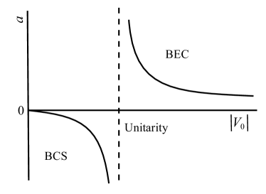
Figure 1: The $s$-wave scattering length $a$ as a function of the microscopic interaction strength $V_{0}$. Here $V_{0}$ is negative, since we are considering an attractive interaction.

For $a>0$ the microscopic interaction has a bound state with an energy $E=-\hbar^{2}/ma^{2}$. This is the single-channel picture of a Feshbach resonance. In this paper we focus on the unitarity limit and on the BCS side of the resonance. Thus, we look at the case where $a$ diverges and at negative scattering lengths $a$. For those scattering lengths we can use the single-channel picture, as long as the Feshbach resonance is sufficiently broad. Namely, in the limit of a broad resonance the amplitude to be in the bare molecular state of the Feshbach resonance turns out to be very small Romans ; Partridge .

III Landau Theory of Phase Transitions

In order to study the critical behavior of a system, in our case an imbalanced Fermi gas, we consider the Landau thermodynamic potential density $\omega_{\text{L}}(\Delta(\mathbf{x}))$, with $\Delta(\mathbf{x})$ the superfluid order parameter. Near the phase transition, where the BCS order parameter $\Delta(\mathbf{x})$ is small, the Landau thermodynamic potential density can be expanded as Negele ; uqf

$$\omega_{\text{L}}(\Delta;\mu_{\sigma},T)=\gamma|\nabla\Delta|^{2}+\alpha|\Delta|^{2}+\frac{\beta}{2}|\Delta|^{4}+\ldots,$$ (8)

where the dots denote the higher orders in $|\Delta|^{2}$ and in gradients $|\nabla\Delta|^{2}$. The Landau coefficients in the thermodynamic potential all depend on the temperature and on the chemical potentials of the two fermion species. If in the thermodynamic potential all coefficients are positive, the minimum of the thermodynamic potential is located at $\langle\Delta(\mathbf{x})\rangle$ equal to zero and the system will be in the normal state. Whereas a phase transition to a superfluid state has occurred when the position of the global minimum is located at a nonzero order parameter $\langle\Delta(\mathbf{x})\rangle$, which describes a condensate of bosonic pairs. In the case that $\gamma$ is positive, it costs energy to have a spatially varying superfluid. It is then energetically favorable for the system to be homogeneous and therefore we can restrict ourselves to a pairing field $\Delta$ independent of position.

We consider first the case where $\gamma$ is positive and the system is homogeneous. For high temperatures all coefficients in the thermodynamic potential will be positive and the system will be in the normal state. But for low temperatures it can occur that certain coefficients change sign. Suppose that in the Landau thermodynamic potential $\alpha$ is negative and all other coefficients are positive. The minimum of the thermodynamic potential will then be attained at some nonzero $\langle\Delta\rangle$ and the Fermi gas will be in the superfluid state. Thus, as $\alpha$ changes sign a phase transition takes place. The temperature at which the transition from the normal state to the superfluid state occurs, for given chemical potentials, can be determined by equating the quadratic coefficient to zero, $\alpha(T_{\text{c}})=0$, where $T_{\text{c}}$ is called the critical temperature. The phase transition just described is called a second-order phase transition and it is characterized by the fact that the minimum of the thermodynamic potential shifts away from zero continuously, see Fig. 2a.

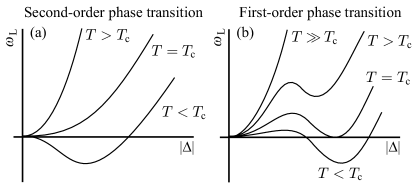
Figure 2: The thermodynamic potential density $\omega_{\text{L}}(|\Delta|)$ as a function of the order parameter $\Delta$. Panel (a) shows the behavior of $\omega_{\text{L}}(|\Delta|)$ for different temperatures when a second-order phase transition occurs and panel (b) when a first-order phase transition occurs.

It is also possible to have a first-order phase transition. To explain a first-order phase transition we consider the situation where in the thermodynamic potential density all coefficients but the fourth-order coefficient $\beta$ are positive. The thermodynamic potential will then typically have two minima. One of these is located at $\Delta$ equal to zero and the other one will be located at a nonzero value of the order parameter. For higher temperatures the minimum located at zero is a global minimum and the Fermi gas is in the normal state. If the temperature is lowered there will be a point where the two minima are equal and for even lower temperatures the minimum located at a nonzero order parameter $\langle\Delta\rangle$ is the global minimum. The system is then in the superfluid state. The first-order phase transition takes place when these two minima are equal, i.e., when $\omega_{\text{L}}(0)=\omega_{\text{L}}(\langle\Delta\rangle)$. In contrast to a second-order phase transition, the location of the global minimum of the thermodynamic potential now changes discontinuously from being zero to a nonzero $\langle\Delta\rangle$, see Fig. 2b.

Next, we consider the case where $\gamma$ is negative. The system can then gain energy when the order parameter varies in space. Thus, instead of being constant, the order parameter will now depend on position. Fulde and Ferrell studied the plane-wave solution Fulde

$$\Delta(\mathbf{x})=\Delta_{0}e^{\text{i}\mathbf{k\cdot x}},$$ (9)

while Larkin and Ovchinnikov considered a superfluid with the single standing-wave order parameter Larkin

$$\Delta(\mathbf{x})=\Delta_{0}\cos(\mathbf{k\cdot x}),$$ (10)

which turns out to be energetically more favorable than the plane-wave case. Superpositions of more than two plane waves are also possible.

In the LO phase the wavefunction of the bosonic pairs is periodic and therefore there will also exist a periodicity in the atomic density. This periodic structure shows itself in the diagonal elements of the one-particle density matrix $n(\mathbf{x},\mathbf{x^{\prime}})$ and is therefore called diagonal long-range order. This diagonal long-range order is what characterizes a solid. In a fermionic superfluid a fraction of the Cooper pairs is in the lowest energy eigenstate. There thus exists a long-range order between the positions of the pairs. It is also said that the two-particle density matrix $g(\mathbf{x},\mathbf{x^{\prime}})$ has off-diagonal long-range order, which implies that $g(\mathbf{x},\mathbf{x^{\prime}})$ does not vanish in the limit $|\mathbf{x}-\mathbf{x^{\prime}}|\rightarrow\infty$ and characterizes a superfluid. In the case where $\gamma$ is negative a transition occurs from the normal state to a superfluid where the atomic density in the superfluid has a periodic structure. Then there exists both diagonal long-range order as well as off-diagonal long-range order and the state is both solid and superfluid. This is called a supersolid phase Bulgac ; uqf .

Further on, we show that in a mass-imbalanced Fermi gas not only a second-order phase transition can occur, but also a first-order transition and even a transition to an inhomogeneous superfluid, depending on the values of the two chemical potentials. Therefore, there must be points in the phase diagram where the character of the phase transition changes. If the phase transition changes from being second order to first order there will be a tricritical point Chaikin . This point can thus be found by setting

$$\alpha(T_{\text{c}3})=\beta(T_{\text{c}3})=0,$$ (11)

where $T_{\text{c}3}$ is the tricritical temperature. For temperatures higher than the tricritical temperature the phase transition from the normal to the superfluid state is of second order, while for $T<T_{\text{c}3}$ there is a first-order phase transition and phase separation occurs.

The phase transition could also change from being a transition from the normal state to a homogeneous superfluid to a transition from the normal state to a supersolid. The point in the phase diagram where this occurs is called a Lifshitz point Chaikin . This point can be computed by demanding

$$\alpha(T_{\text{L}})=\gamma(T_{\text{L}})=0,$$ (12)

where $T_{\text{L}}$ is called the Lifshitz temperature. For temperatures lower than the Lifshitz temperature the transition will be from a normal state to a superfluid state where the bosonic pairs have a nonzero momentum. Superfluidity at nonzero momentum can be established in many ways and due to this variety of possibilities it is difficult to predict which kind of superfluidity will be present below the Lifshitz point. However, they all have to emerge from the Lifshitz point and therefore it is important to know the position of the Lifshitz point.

Apart from the above two possibilities, we can think of other scenarios for the change in character of the phase transitions. But in the phase diagrams we calculated for the imbalanced Fermi gas we only found tricritical points and Lifshitz points. Therefore, these are the only two possibilities we discuss in the following.

IV Mean-Field Theory

In this section we present the mean-field thermodynamic potential, which is an approximation to the exact Landau thermodynamic potential for the Fermi gas with population and mass imbalance. If we have an expression for the Landau thermodynamic potential, we are able to determine the phase diagram.

Although mean-field theory does not contain all interactions present in a Fermi mixture, it turns out that mean-field theory already incorporates all the relevant physics determining the topology of the phase diagrams. Adding fluctuation effects only changes the phase diagrams quantitatively prl ; Koos ; Gorkov ; Iskin . Because of the rather straightforward and transparent calculations in mean-field theory, we first discuss mean-field theory in some detail. Later on we take fluctuation effects into account in order to obtain more quantitative results which we can compare with Monte Carlo calculations and for the mass-balanced case with experiment.

IV.1 Thermodynamic Potential

We consider a two-component Fermi mixture, i.e., a mixture containing either a single fermionic species, for which two different hyperfine states are present, or consisting of two different fermionic species with access to a single hyperfine state. A balanced Fermi gas consists of a single species with an equal population of both spin states. In an imbalanced Fermi gas we allow the populations and masses to be different. To take into account a population imbalance we use different chemical potentials for the two (pseudo)spin states, while a mass imbalance implies that the particles in the two hyperfine states have different masses. The chemical potential and the mass of the fermions in state $|\sigma\rangle$ will be denoted by $\mu_{\sigma}$ and $m_{\sigma}$ respectively. From now on heavy particles are always denoted by a minus sign and light particles by a plus sign, thus $\sigma=\pm$.

The mean-field thermodynamic potential for the imbalanced Fermi gas is given by

$$\omega_{\text{L}}(|\Delta|)=-\frac{|\Delta|^{2}}{T^{\text{2B}}(0)}+\int\frac{\text{d}\mathbf{k}}{(2\pi)^{3}}\Big{\{}\varepsilon(\mathbf{k})-\mu-\hbar\omega(\mathbf{k})$$

$$+\frac{|\Delta|^{2}}{2\varepsilon(\mathbf{k})}-\frac{1}{\beta}\sum_{\sigma}\log\left(1+e^{-\beta\hbar\omega_{\sigma}(\mathbf{k})}\right)\Big{\}},$$ (13)

where the two-body transition matrix $T^{\text{2B}}(0)$ is given by Eq. (6). This thermodynamic potential is a direct generalization of the thermodynamic potential for a balanced Fermi gas uqf ; Fetter . In the above expression $\beta=1/k_{\text{B}}T$ is the inverse thermal energy, $\mu=(\mu_{+}+\mu_{-})/2$ is the average chemical potential and half the reduced kinetic energy is $\varepsilon(\mathbf{k})=(\varepsilon_{+}(\mathbf{k})+\varepsilon_{-}(\mathbf{k}))/2$ with

$$\varepsilon_{\sigma}(\mathbf{k})=\frac{\hbar^{2}\mathbf{k}^{2}}{2m_{\sigma}}.$$ (14)

The first terms in the above thermodynamic potential represent the BCS ground state of the mixture, where $\hbar\omega(\mathbf{k})$ is the average dispersion of the quasiparticles

$$\hbar\omega(\mathbf{k})=\sqrt{(\varepsilon(\mathbf{k})-\mu)^{2}+|\Delta|^{2}},$$ (15)

with $|\Delta|$ the so called BCS gap parameter. The complex pairing field $\Delta$ is on average related to the expectation value of the pair annihilation operator through

$$\left<\Delta(\mathbf{x})\right>=V_{0}\left<\hat{\psi}_{-}(\mathbf{x})\hat{\psi}_{+}(\mathbf{x})\right>,$$ (16)

with $\hat{\psi}_{\sigma}(\mathbf{x})$ the fermionic annihilation operators.

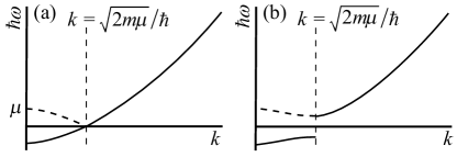
Figure 3: The single-particle dispersions $\hbar\omega_{\sigma}(\mathbf{k})$ for the balanced Fermi gas. Panel (a) shows the dispersions for zero $\Delta$ where the system is in the normal state. Panel (b) depicts the case where the system is in the superfluid state, thus the dispersions for nonzero $\Delta$. In both panels the dashed lines are the dispersions of the hole-like excitations, while the full lines give the particle-like dispersions. The latter show more clearly the opening of a gap $2\Delta$ at the Fermi level due to the formation of a condensate of Cooper pairs.

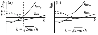
Figure 4: The dispersions $\hbar\omega_{\sigma}(\mathbf{k})$ for the Fermi gas with both population and mass imbalance. Panel (a) shows again the dispersions for zero $\Delta$ where the system is in the normal state. And panel (b) again depicts the case where the system is in the superfluid state, thus the dispersions for nonzero $\Delta$. The meaning of the dashed and full lines are the same as for Fig. 3.

The second part of the thermodynamic potential, namely the part containing the logarithms, corresponds to the contribution of an ideal gas of quasiparticles. Here, $\hbar\omega_{\sigma}(\mathbf{k})$ is the dispersion relation of the quasiparticles in state $|\sigma\rangle$, given by

$$\hbar\omega_{\sigma}(\mathbf{k})=\hbar\omega(\mathbf{k})-\sigma[2h-\varepsilon_{+}(\mathbf{k})+\varepsilon_{-}(\mathbf{k})]/2,$$ (17)

with $h=(\mu_{+}-\mu_{-})/2$ the difference in chemical potentials. For the unpolarized Fermi gas with equal masses the dispersions $\hbar\omega_{\sigma}(\mathbf{k})$ reduce to the average dispersion in Eq. (15). This dispersion is plotted in Fig. 3 for both the normal state (Fig. 3a) and the superfluid state (Fig. 3b). In this case the superfluid is gapped and balanced. For $k=|\mathbf{k}|<\sqrt{2m\mu}/\hbar$ the quasiparticle dispersion describes hole-like excitations. If we mirror this hole-like part of the quasiparticle dispersion, we obtain the negative dispersion of the particle-like excitations. For $k>\sqrt{2m\mu}/\hbar$ the quasiparticle dispersion already describes the particle-like excitations.

In the case of a polarized superfluid with equal masses the dispersions $\hbar\omega_{\sigma}(\mathbf{k})$ in Fig. 3 are shifted by the difference in chemical potentials $2h$. For $h>|\Delta|$ the dispersion of the majority species becomes negative. When this occurs, the occupation of the single-particle states associated with the negative part of the quasiparticle excitation branch actually lowers the ground-state energy. Since this leads to additional majority quasiparticles and, therefore, additional majority particles and minority holes, in the ground state, the ground state becomes a polarized superfluid. The resulting gapless and polarized superfluid is called the Sarma phase Sarma . For the Fermi gas with both mass and population imbalance the dispersions are depicted in Fig. 4, where Fig. 4a shows the dispersions for zero $\Delta$ and Fig. 4b for nonzero $\Delta$. The shape of the dispersions is changed due to the difference in mass. It can be seen that in this case also one of the dispersions, namely $\hbar\omega_{-}(\mathbf{k})$, is negative so that it would correspond to a gapless Sarma superfluid.

IV.2 Landau Coefficients

For the imbalanced Fermi mixture, we want to study the phase transition from the normal state to the superfluid state. For that transition we want to obtain a phase diagram with the critical temperature as a function of the polarization, $P=(n_{+}-n_{-})/(n_{+}+n_{-})$ with $n_{\sigma}$ the density of particles in state $|\sigma\rangle$.

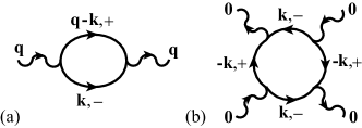
Figure 5: (a) The ladder diagram with external momentum $\mathbf{q}$. The wiggly lines denote the Cooper pairs, which can break up into two fermions of different spin, denoted by the normal lines. Here, $\mathbf{q}$ is the wavevector of the Cooper pairs, while $\mathbf{k}$ and $\mathbf{q}-\mathbf{k}$ are the wavevectors of the fermions. When $\mathbf{q}$ is equal to zero, the amplitude of this diagram corresponds to the quadratic Landau coefficient $\alpha$ in the thermodynamic potential. (b) The Feynman diagram corresponding to the fourth-order Landau coefficient $\beta$.

The particle densities $n_{\sigma}$ can be determined from the thermodynamic potential using uqf

$$n_{\sigma}=\left.-\frac{\partial\omega_{\text{L}}(\Delta)}{\partial\,\mu_{\sigma}}\right|_{\Delta=\langle\Delta\rangle}.$$ (18)

Moreover, in Sec. III the critical conditions for the transition were explained. In mean-field theory, the quadratic Landau coefficient $\alpha$ is explicitly given by

$$\alpha=\left.\frac{\partial\omega_{\text{L}}}{\partial|\Delta|^{2}}\right|_{|\Delta|^{2}=0}=-\frac{1}{T^{\text{2B}}(0)}$$

$$+\int\frac{\text{d}\mathbf{k}}{(2\pi)^{3}}\left(\frac{1}{2\varepsilon(\mathbf{k})}+\frac{N_{+}(\mathbf{k})+N_{-}(\mathbf{k})-1}{2(\varepsilon(\mathbf{k})-\mu)}\right),$$ (19)

where $N_{\sigma}(\mathbf{k})=1/(\exp[\beta(\varepsilon_{\sigma}(\mathbf{k})-\mu_{\sigma})]+1)$ are the Fermi distribution functions. To determine the temperature of the tricritical point, we also need to know the fourth-order Landau coefficient $\beta$. It is given by

$$\beta=\left.\frac{\partial^{2}\omega_{\text{L}}}{(\partial|\Delta|^{2})^{2}}\right|_{|\Delta|^{2}=0}=\int\frac{\text{d}^{3}\mathbf{k}}{(2\pi)^{3}}\frac{1}{4(\varepsilon(\mathbf{k})-\mu)^{2}}$$

$$\noindent\times\Bigg{[}\beta N_{+}(\mathbf{k})(N_{+}(\mathbf{k})-1)+\beta N_{-}(\mathbf{k})(N_{-}(\mathbf{k})-1)$$

$$\noindent\hskip 11.38109pt+\frac{1}{\varepsilon(\mathbf{k})-\mu}(1-N_{+}(\mathbf{k})-N_{-}(\mathbf{k}))\Bigg{]}.$$ (20)

Determining $\gamma$ from the mean-field thermodynamic potential is not possible, since we have assumed the bosonic pairing field $\Delta(\mathbf{x})$ to be independent of position. Nevertheless, there is a rather simple way to determine this coefficient, using Feynman diagrams Kleinert . The other coefficients could also have been determined using a diagrammatic language. Namely, the quadratic coefficient $\alpha$ corresponds to the so called ladder diagram where the incoming and outgoing bosonic fields $\Delta$ have zero momentum, see Fig. 5a. Physically, $\alpha$ can be interpreted as being proportional to the chemical potential of the Cooper pairs. The fourth-order coefficient $\beta$ has a diagrammatic representation with four external bosonic fields with zero momentum, see Fig. 5b.

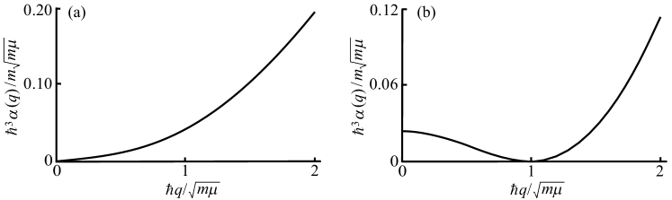
Figure 6: Depending on the temperature and the chemical potentials, the minimum of $\alpha(\mathbf{q})$ is either at zero or at nonzero external momentum $\hbar q$. In both pictures the mass ratio is $r=6.7$. In panel (a), the minimum of $\alpha(\mathbf{q})$ is located at zero external momentum. The corresponding polarization is $P=-0.61$ and the temperature is $T/T_{\text{F}}=0.21$ with $T_{\text{F}}$ the Fermi temperature. In panel (b), the minimum of $\alpha(\mathbf{q})$ is attained at a nonzero momentum. Here the polarization is $P=-0.7$ and the temperature is $T/T_{\text{F}}=0.13$.

For the transition to the supersolid phase, we consider the ladder diagram where the bosonic fields carry nonzero momentum $\mathbf{q}$, since the supersolid phase consists of bosonic pairs with nonzero momentum. The expression for this ladder diagram is

$$\alpha(\mathbf{q})=-\frac{1}{T^{\text{2B}}(0)}+\int\frac{\text{d}^{3}\mathbf{k}}{(2\pi)^{3}}\Bigg{\{}\frac{1}{2\varepsilon(\mathbf{k})}+$$

$$\frac{N_{+}(\mathbf{q-k})+N_{-}(\mathbf{k})-1}{\varepsilon_{+}(\mathbf{q-k})+\varepsilon_{-}(\mathbf{k})-2\mu}\Bigg{\}}.$$ (21)

The actual shape of $\alpha(\mathbf{q})$ as a function of the external momentum $\mathbf{q}$ depends on the values of the different parameters in this expression, such as the chemical potentials and the temperature. Depending on those quantities the minimum of $\alpha(\mathbf{q})$ is attained either for zero or for nonzero external momentum. As explained in Sec. III, a second-order phase transition can occur, when a quadratic coefficient of the Landau theory changes sign. These coefficients are now given by $\alpha({\bf q})$, where ${\bf q}$ is the wavevector of the bosonic pairs. The sign change occurs first for the minimum of $\alpha({\bf q})$, which therefore determines whether or not the transition happens at nonzero ${\bf q}$. The expression for the ladder diagram with nonzero external momentum can be expanded in even powers of $\mathbf{q}$

$$\alpha(\mathbf{q})=a_{0}+a_{1}\mathbf{q}^{2}+a_{2}\mathbf{q}^{4}+\ldots,$$ (22)

where the dots denote higher order powers in $\mathbf{q}^{2}$. If all the coefficients $a_{i}$ are positive, $\alpha(\mathbf{q})$ has a minimum for external momentum zero, so that a transition to the homogeneous superfluid phase occurs. But if $a_{1}$ is negative, $\alpha(\mathbf{q})$ has a minimum for a nonzero external momentum and therefore it first becomes zero at some nonzero value of $\mathbf{q}$. The minimum of the thermodynamic potential will then be located at a nonzero order parameter with a nonzero momentum. In other words, it will be energetically favorable for the bosonic pairs to have kinetic energy and the phase transition that occurs is a transition from the normal state to an inhomogeneous superfluid. Comparing this with the Landau theory of Sec. III, we see that in the expansion of $\alpha(\mathbf{q})$, $a_{0}$ can be identified with the quadratic coefficient $\alpha$ and $a_{1}$ can be identified with $\gamma$. Thus, from the ladder diagram with external momentum an expression for $\gamma$ can be found, namely

$$\gamma=\left.\frac{\partial\alpha(\mathbf{q})}{\partial\mathbf{q}^{2}}\right|_{\mathbf{q}=0}.$$ (23)

Physically, $\gamma$ can be interpreted as being proportional to the inverse of the effective mass of the Cooper pairs.

IV.3 Results

In this section the results using mean-field theory are presented. First, we present phase diagrams for three Fermi gases with different mass imbalances. Then, we study the effect of the mass imbalance on the critical temperature for an unpolarized Fermi gas. After this, we study the effect of the interaction strength on the temperature corresponding to a tricritical point or a Lifshitz point. Finally, we also consider the superfluid Sarma phase.

IV.3.1 Phase Diagrams

With the expressions for the Landau coefficients, the phase diagram can be calculated for a fixed mass ratio $r$ and a fixed interaction strength $1/k_{\text{F}}a$. We determine the phase diagram as a function of temperature $T$ and polarization $P=(n_{+}-n_{-})/(n_{+}+n_{-})$. The mass ratio $r$ is given by $r=m_{-}/m_{+}$. The interaction strength is characterized by the $s$-wave scattering length $a$ and the Fermi momentum $k_{\text{F}}$, which is defined as

$$k_{\text{F}}=(3\pi^{2}n)^{1/3},$$ (24)

where $n=n_{+}+n_{-}$ is the total particle density. In order to obtain a phase diagram independent of the total particle density $n$, we scale the temperature with the reduced Fermi temperature

$$k_{\text{B}}T_{\text{F}}=\varepsilon_{\text{F}}=\frac{\hbar^{2}k_{\text{F}}^{2}}{2m},$$ (25)

where $m$ is twice the reduced mass, introduced in Eq. (5) and $k_{\text{B}}$ is Boltzmann’s constant.

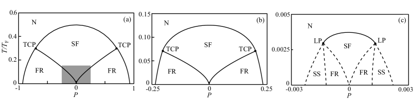
Figure 7: Phase diagrams of the mass-balanced Fermi gas, $r=1$, as a function of temperature $T$ and polarization $P$ at different interaction strengths. The temperature is scaled with the Fermi temperature $T_{\text{F}}$. Panel (a) shows the phase diagram in the strongly interacting limit, $1/k_{\text{F}}a=0$. There is a tricritical point (TCP), where the normal state (N), the homogeneous superfluid state (SF) and the forbidden region (FR) meet. The shaded area sets the scale for panel (b), where the phase diagram for a weaker interaction, $1/k_{\text{F}}a=-1$, is shown. Again, there is a tricritical point. There is again a shaded region to set the scale for panel (c), but it is too small to see. In panel (c) the phase diagram is shown for a very weak interaction, $1/k_{\text{F}}a=-3$, and the critical temperatures are now extremely low. For this interaction we find a Lifshitz point (LP), below which there is an instability towards a supersolid (SS). The size of this supersolid region is not calculated within our theory and therefore the dashed lines are only guides to the eye.

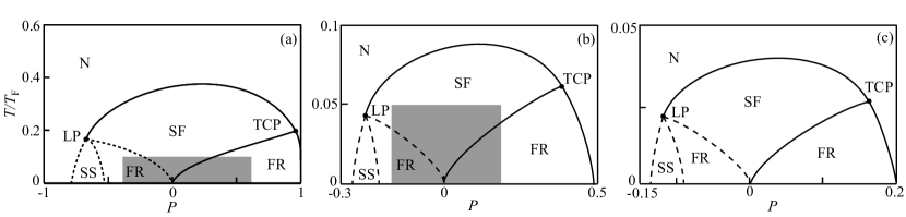
Figure 8: Phase diagrams of the Fermi gas with mass ratio $r=6.7$ for different interaction strengths. Panel (a) shows the phase diagram in the strongly interacting limit. The size of the box is the same as for the mass-balanced case such that the effect of the mass imbalance can be seen. The shaded region sets the scale for panel (b), where the interaction strength is weaker, $1/k_{\text{F}}a=-1$. And in panel (b) the shaded region in turn sets the scale for panel (c) where the interaction is even weaker, $1/k_{\text{F}}a=-3/2$. The dashed lines are again guides to the eye.

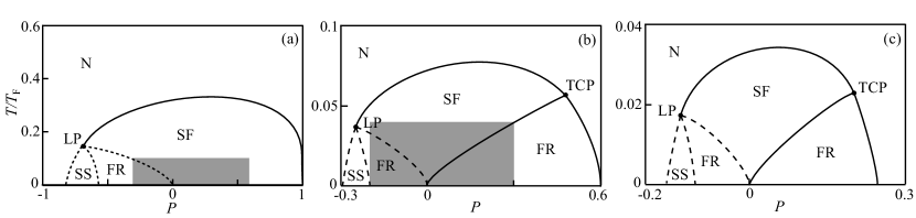
Figure 9: Phase diagrams of the Fermi gas with mass ratio $r=10$ for different interaction strengths. Again, panel (a) shows the phase diagram in the strongly interacting limit and the size of the box is again the same as for the mass-balanced case. The shaded region sets the scale for panel (b), where the interaction strength is weaker, $1/k_{\text{F}}a=-1$. And in panel (b) the shaded region in turn sets the scale for panel (c) where the interaction is even weaker, $1/k_{\text{F}}a=-3/2$. Again, the dashed lines are only guides to the eye.

We present the phase diagram for three different mass ratios, namely for $r=1$, which is the mass-balanced case, $r=6.7$, which corresponds to a ⁶Li-⁴⁰K mixtures, and for $r=10$ where an interesting feature in the phase diagram is found regarding the tricritical point Parish . For these mass ratios we present the phase diagrams at three different interaction strengths in order to see what the effect of the interaction is on the critical temperature. Namely, we present the phase diagrams for a strongly interacting Fermi gas with $1/k_{\text{F}}a=0$, an intermediate interaction strength with $1/k_{\text{F}}a=-1$ and a weakly interacting Fermi gas. These interaction strengths correspond to the BCS side of the Feshbach resonance, see Fig. 1.

Fig. 7 shows the phase diagrams of the mass-balanced Fermi gas at three different interaction strengths. In Fig. 7a the phase diagram for the strongly interacting regime where $1/k_{\text{F}}a=0$ is depicted. It is symmetric in the polarizations. The phase transition is of second order for small polarizations. Moreover, we find two tricritical points in the phase diagram and below the tricritical points the phase transition is of first order. At a first-order phase transition the order parameter is discontinuous and therefore also the particle densities $n_{\sigma}$, see Eq. (18). And thus also the polarization is discontinuous at a first-order phase transition, which gives rise to a forbidden region where phase separation occurs. Fig. 7b again shows the phase diagram of the mass-balanced Fermi gas, but now for a weaker interaction, namely for $1/k_{\text{F}}a=-1$. Compared to the unitarity regime, there are no qualitative changes in the phase diagram. However, the critical temperatures are lower than in the strongly interacting regime. Then, Fig. 7c shows the phase diagram of the mass-balanced Fermi gas for a very weak interaction, namely $1/k_{\text{F}}a=-3$. Apart from the fact that the critical temperatures are now extremely low, there is a large difference compared to the strongly interacting regime, namely we do not find tricritical points in the phase diagram but instead we find two Lifshitz points. Below the Lifshitz point there is an instability towards supersolidity. We assumed that there will be a second-order transition from the normal state to the supersolid. The critical temperature for this transition is found by solving $\alpha(\mathbf{k}_{\text{LO}})=0$, where $\mathbf{k}_{\text{LO}}$ is the wavevector of the supersolid. The transition from supersolidity to the homogeneous superfluid phase is expected to be first order Casalbuoni ; Mora and thus a forbidden region will be present in the phase diagram. This simple scenario is sketched in the phase diagram, but it could be that the normal to supersolid second-order phase transition is preempted by weak first-order transitions from the normal state to various more complicated supersolid phases Casalbuoni ; Mora ; Yip . For the calculation of the relevant fourth-order diagrams with nonzero external momenta, one needs to make an assumption about the crystal structure of the supersolid phase, in order to calculate a first-order phase transition to the supersolid phase. This calculation for the stability regions of all possible supersolid phases is beyond the scope of this paper. To emphasize that we did not investigate this region in great detail we there used dashed lines in the phase diagram.

Fig. 8 again shows three phase diagrams at different interactions, but now for the mass-imbalanced Fermi gas with mass ratio $r=6.7$, corresponding to the ⁶Li-⁴⁰K Fermi mixture. In the unitarity regime, see Fig. 8a, the phase diagram is no longer symmetric in polarizations and the temperatures are lower in comparison with the mass-balanced case. Furthermore, already in the strongly interacting regime we find a Lifshitz point in the phase diagram for a majority of heavy atoms. For a majority of light particles a tricritical point is found. This is in sharp contrast with the mass-balanced case where a Lifshitz point is only present for extremely weak interactions. As a result, the Lifshitz temperature is then at least about a hundred times lower than for the ⁶Li-⁴⁰K mixture. Below the tricritical point there is a forbidden region and below the Lifshitz point there is an instability towards a supersolid. We sketched the same scenario below the Lifshitz point here as for the mass-balanced case. In Fig. 8b and Fig. 8c the phase diagrams of the Fermi gas are depicted at interaction strengths $1/k_{\text{F}}a=-1$ and $1/k_{\text{F}}a=-3/2$ respectively. The interaction strength does not affect the topology of the phase diagram, but it does affect the critical temperatures. Just as in the mass-balanced case, the critical temperatures are lower for weaker interactions, as expected.

In Fig. 9 we show the phase diagrams of an imbalanced Fermi gas with an even larger mass imbalance, namely with mass ratio $r=10$. The diagram has become even more asymmetric. In the strongly interacting regime, we also find a Lifshitz point for a majority of heavy atoms. But the tricritical point has disappeared, which means that the phase transition remains of second order and no phase separation occurs for a majority of light particles. Below the Lifshitz point the same scenario is sketched as before. Fig. 9b shows the phase diagram at a weaker interaction strength, namely at $1/k_{\text{F}}a=-1$. With respect to the unitarity limit there is a real change in this diagram. Namely, the tricritical point reappears in the phase diagram. Then, in Fig. 9c the interaction strength is even weaker, $1/k_{\text{F}}a=-3/2$, and the critical temperatures are lower. But there are no qualitative changes with respect to the phase diagram in Fig. 9b.

IV.3.2 Effect of a Mass Imbalance

By comparing the phase diagrams of the mass-balanced Fermi gas and of the Fermi gases with a mass imbalance, it can be seen that a mass imbalance causes important changes. First, the critical temperatures for the mass-imbalanced Fermi gases are lower than for the mass-balanced case. Second, for a mass-imbalanced Fermi gas the phase diagram is no longer symmetric in polarizations. In other words, the maximum critical temperature is no longer located at zero polarization. Third, for Fermi gases with a sufficiently large mass ratio, like the two mass-imbalanced Fermi gases we presented here, there is a Lifshitz point in the phase diagram for a majority of heavy atoms. These three changes we now discuss in some more detail.

In the weakly interacting limit, the critical temperatures are very low. For the unpolarized Fermi gas the integral in Eq. (19) can then be evaluated exactly. Then, by equating $\alpha$ to zero an analytic result for the critical temperature can be obtained Paananen

$$\left.T_{c}\right|_{P=0} =\sqrt{\varepsilon_{\text{F},+}\varepsilon_{\text{F},-}}\frac{8}{\pi k_{\text{B}}}e^{\gamma-2}e^{-\pi/2k_{\text{F}}|a|}$$

$$=\frac{2\sqrt{r}}{1+r}\frac{8\varepsilon_{\text{F}}}{\pi k_{\text{B}}}e^{\gamma-2}e^{-\pi/2k_{\text{F}}|a|},$$ (26)

where $\varepsilon_{\text{F}}$ is the Fermi energy corresponding to twice the reduced mass, $k_{\text{B}}$ is Boltzmann’s constant and $\gamma=0.5772$ is Euler’s constant. When the atoms making up the Fermi mixture have different masses, $r$ is not equal to one. In that case the term $2\sqrt{r}/(1+r)$ is smaller than one. And thus, by adding a mass imbalance the critical temperature for the unpolarized Fermi gas becomes lower. In Fig. 10, it can be seen that the dependence of the critical temperature on the mass ratio is indeed as given by Eq. (26) and that the agreement with the numerical results is very good. For the polarized Fermi gas, we expect a similar dependence of the critical temperature on the mass ratio.

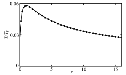
Figure 10: The critical temperature of an unpolarized Fermi gas as a function of the mass ratio $r=m_{-}/m_{+}$. The circles are the numerical results of $\alpha=0$ and the full line is the analytic result for the weakly interacting limit. Here $1/k_{\text{F}}a=-3/2$.

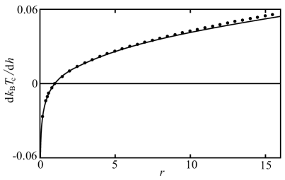
Figure 11: Derivative of the critical temperature with respect to the difference in chemical potentials $h$. The circles are the numerical results and the full line is the analytic result. The interaction strength is $1/k_{\text{F}}a=-3/2$.

For the mass-balanced Fermi gas, the highest critical temperature is located at zero polarization, see Fig. 7, whereas for the mass-imbalanced Fermi gas it is located at nonzero polarization, see Fig. 8 and Fig. 9. As a consequence, the derivative of the critical temperature with respect to $h$, the difference in chemical potentials, will no longer be zero at $P=0$. In the weakly interacting limit, the coefficient $\alpha$ in Eq. (19) can be expanded around the critical temperature $T_{c}$ and the critical ‘Zeeman’ field $h_{0}$ corresponding to the unpolarized Fermi gas

$$\alpha(T_{c}+\delta T_{c},h_{0}+\delta h)\simeq$$

$$\alpha(T_{c},h_{0})+\frac{\partial\alpha}{\partial T}(T_{c},h_{0})\delta T_{c}+\frac{\partial\alpha}{\partial h}(T_{c},h_{0})\delta h.$$ (27)

For a continuous phase transition, $\alpha$ has to go to zero. The term on the left-hand side and the first term on the right-hand side are therefore zero. Then we find from the other two terms

$$\left.\frac{\delta T_{c}}{\delta h}\right|_{P=0} =-\frac{\partial\alpha/\partial h}{\partial\alpha/\partial T}=\left.T_{c}\right|_{P=0}\frac{1}{4}\left(\frac{1}{\varepsilon_{\text{F},-}}-\frac{1}{\varepsilon_{\text{F},+}}\right)$$

$$=\frac{2}{\pi k_{\text{B}}}\frac{r-1}{\sqrt{r}}e^{\gamma-2}e^{-\pi/2k_{\text{F}}|a|}.$$ (28)

This is indeed nonzero if the mass ratio is not equal to one. Eq. (28) is positive for mass ratios larger than one. This is in agreement with our findings that the phase diagram shifts towards positive polarizations for a mass ratio larger than one, see Fig. 8 and Fig. 9. For mass ratios smaller than one, Eq. (28) is negative and the phase diagram then shifts towards negative polarizations. In both cases the phase diagram shifts towards a majority of light particles. Eq. (28) is plotted in Fig. 11, together with the numerical results. The agreement is good, especially for small mass ratios.

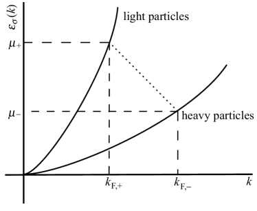
Figure 12: The energies $\varepsilon_{\sigma}(k)$ of the fermions for a Fermi mixture with both a population and a mass imbalance, where $m_{-}>m_{+}$ and $n_{-}>n_{+}$. Thus, there is a majority of heavy particles. At the Fermi levels, the energy difference between particles with different momenta (dashed line) is smaller than the energy difference between particles with the same momenta.

For a sufficiently large mass ratio we find a Lifshitz point in the phase diagram for a majority of heavy particles. To explain why this can be expected we consider the kinetic energies of the particles in Eq. (14), which are plotted in Fig. 12. In the mass-balanced case a fermion of one species with momentum $\mathbf{k}$ has the same energy as a fermion with momentum $-\mathbf{k}$ of the other species. Coupling these degenerate states by a condensate of Cooper pairs is energetically desirable since the shift of the energy levels due to the coupling is now largest, as is well-known from the physics of avoided crossings. Therefore, it is thus most favorable to form a pair of two fermions with the same but opposite momentum, i.e., a fermion with momentum $\mathbf{k}$ forms a pair with a fermion with momentum $-\mathbf{k}$, since then the energy gain as a result of pairing is maximal. The pair then has no kinetic energy and the pairs form a homogeneous superfluid.

Typically, the formation of pairs mostly occurs at the Fermi energy. There a pair consists of one fermion with momentum $\mathbf{k}_{\text{F}}$ and one with momentum $-\mathbf{k}_{\text{F}}$. Since the Fermi momentum depends on the density of the particles $n_{\sigma}$, see Eq. (24), the Fermi momenta will not be the same in the case of a population imbalance. This makes pairing less ideal than in the unpolarized case. The critical temperatures are therefore lower for a polarized mixture, see Fig. 7.

In the mass-imbalanced case two fermions with equal momentum but from different species do not have the same kinetic energy. Thus, if now a fermion of one species with momentum $\mathbf{k}$ forms a pair with a fermion with momentum $-\mathbf{k}$ of the other species, there is an energy difference that reduces the energy gain that can be obtained due to pairing. This explains the fact that the critical temperatures are lower for Fermi mixtures with a mass imbalance. With both a mass imbalance and a population imbalance pairs can still be formed with two fermions with equal but opposite momentum, even though there is an energy difference between the Fermi levels. However, this occurs only if the mass ratio and the population imbalance are not too large. In the extreme case of a large mass imbalance and a large population imbalance a more favorable scenario is possible, see Fig. 12. In this figure the kinetic energies are plotted for the different fermions, and there is a majority of heavy particles, thus $k_{\text{F},-}>k_{\text{F},+}$. It can be seen that the energy difference between particles with different momenta is now smaller than the energy difference between fermions with the same momentum, i.e., it is now energetically more favorable to form pairs with a nonzero momentum that allows for a direct coupling of the Fermi levels. The first point where this is the case is the Lifshitz point. There the system becomes a supersolid.

IV.3.3 Multicritical Point

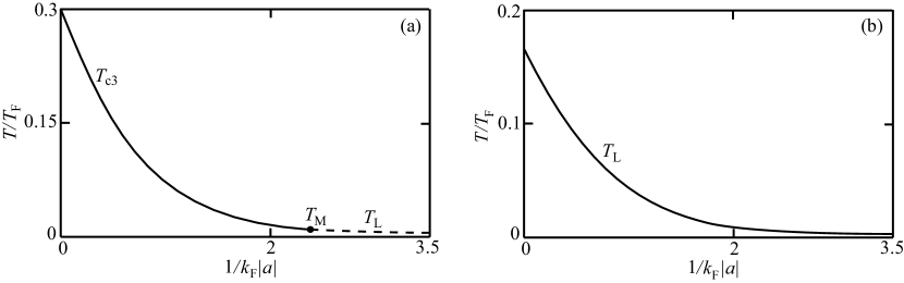
Figure 13: Temperature of the tricritical points and the Lifshitz points as a function of the interaction strength. Panel (a) shows the mass-balanced case. In panel (b) we look at a Fermi gas with mass ratio $r=6.7$ and a majority of heavy particles. $T_{\text{c}3}$ is the temperature of a tricritical point, $T_{\text{M}}$ is the temperature of a multicritical point and $T_{\text{L}}$ of a Lifshitz point.

In the phase diagrams, Fig. 7, Fig. 8 and Fig. 9, we find, depending on the mass ratio and the interaction strength, tricritical points $(P_{\text{c}3},T_{\text{c}3})$, which are solutions of Eq. (11), as well as Lifshitz points $(P_{\text{L}},T_{\text{L}})$, solutions of Eq. (12).

At unitarity, we find for the mass-balanced case at unitarity a tricritical point, whereas we find a Lifshitz point for the ⁶Li-⁴⁰K mixture for a majority of heavy particles. This Lifshitz point is a clearly distinct point from a tricritical point, just as the tricritical point for the mass-balanced case is a clearly distinct point from a Lifshitz point. This is in accordance with the findings of Parish et al. Marchetti , who found that for a mass-balanced Fermi mixture the FFLO line detaches from the tricritical point away from the BCS limit. However, there is a mass ratio between $r=1$ and $r=6.7$ for which the phase diagram at unitarity contains a point which is both a tricritical point and a Lifshitz point. In other words, for this mass ratio Eq. (11) and Eq. (12) have a solution exactly at the same point in the phase diagram. This is a multicritical point and it is found to occur for the mass ratio $r=4.22$.

It can also be seen in the different phase diagrams that for a given mass ratio the location of tricritical and Lifshitz points changes as the interaction strength changes. In Fig. 13, it is shown for the mass-balanced Fermi gas and for the Fermi gas with mass ratio $r=6.7$ how the temperature $T$ of these points changes as a function of the interaction strength. Note that the polarization is not constant for the lines in Fig. 13. In both Fig. 13a and Fig. 13b one can recognize an exponential decay as a function of the interaction strength, which is exactly what one would expect from Eq. (26).

Fig. 13a shows the mass-balanced case. In the unitarity regime and for small values of $1/k_{\text{F}}|a|$ a tricritical point is present in the phase diagram, with temperature $T_{\text{c}3}$. This is the full line in Fig. 13a. Then for some value of the interaction strength Eq. (11) and Eq.(12) have a solution at the same point. Thus, there is a multicritical point and the temperature of this point is in Fig. 13 denoted by $T_{\text{M}}$. For even weaker interactions it then turns out that there is an instability towards a supersolid and thus we find a Lifshitz point in the phase diagram, with temperature $T_{\text{L}}$. This is the dashed line in Fig. 13a.

Although the tricritical and Lifshitz points are very close together for very weak interactions, in our approach, where we perform the momentum integrals to calculate the coefficients $\gamma$ in Eq. (23) and $\beta$ in Eq. (20), they are essentially always two distinct points. Except for one value of the interaction strength where we find a multicritical point. If one, however, assumes particle-hole symmetry in the weakly-interacting limit, Eq. (23) and Eq. (20) become, up to a constant, the same equation and thus one finds that the tricritical point and the Lifshitz point are the same point Casalbuoni ; Buzdin .

Fig. 13b gives the temperature of the Lifshitz point present in the phase diagram of the Fermi gas with mass ratio $r=6.7$ for a majority of heavy particles. Here, we do not find a change in character of the phase transition as a function of interaction strength. The Lifshitz point remains a Lifshitz point. For a majority of light particles of this Fermi mixture, we found a tricritical point in the strongly interacting limit. We expect that this point will also change to a Lifshitz point for very weak interactions, but the extremely low temperatures make it numerically difficult to investigate this possibility in detail.

IV.3.4 Sarma Phase

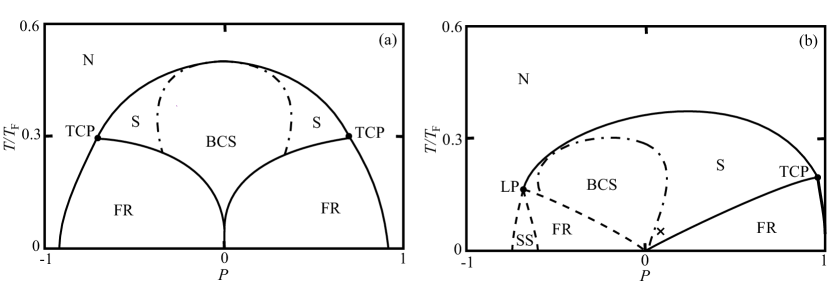
Figure 14: Phase diagrams at unitarity including the region where the superfluid is gapless. Panel (a) shows the mass-balanced case. It is the same phase diagram as in Fig. 8a, only now the superfluid region is divided into a gapped superfluid region (BCS) and two Sarma regions (S). Panel (b) shows the mass-imbalanced Fermi gas with mass ratio $r=6.7$. The small cross in panel (b) is the point at which we calculated the distribution functions of the particles shown in Fig. 15.

In Sec. IVA, while explaining the dispersions of the quasiparticles, we discussed the possibility of a Sarma phase, which occurs when one of the dispersions $\hbar\omega_{\sigma}(\mathbf{k})$ becomes negative. At each point in the phase diagram the value of the order parameter $|\Delta|$ can be found by minimizing the thermodynamic potential in Eq. (13). With this value of the order parameter it can be determined whether the dispersions are always positive or become negative for some range of momenta. In the superfluid phase it turns out that there are different regions. In one region the dispersions are always positive and the superfluid is gapped, while in the other region one of the dispersions becomes negative and we are dealing with a gapless superfluid. At nonzero temperatures, there is no phase transition between these regions. Rather, there is only a smooth crossover. We calculated the gapless superfluid region in the unitarity limit for the mass-balanced case and for the ⁶Li-⁴⁰K Fermi mixture. The results are shown in Fig. 14. In the mass-balanced case, Fig. 14a, there are two regions in the phase diagram where we have a gapless superfluid. In Fig. 14b the mass-imbalanced case is shown. Here, the Sarma region is not symmetric in polarizations, just as the rest of the phase diagram. The Sarma region is very large for positive polarizations, whereas for negative polarizations it becomes very small.

Fig. 15 depicts the distribution functions $N_{\sigma}^{\text{SF}}(\mathbf{k})$ of the heavy and the light particles for some point in the phase diagram of Fig.14b that lies in the superfluid Sarma region. In the superfluid phase the distribution functions are modified with respect to the Fermi distribution functions $N_{\sigma}(\mathbf{k})$ and are given by

$$N_{\sigma}^{\text{SF}}(\mathbf{k}) =\frac{1}{2}\left(1+\frac{\varepsilon(\mathbf{k})-\mu}{\hbar\omega(\mathbf{k})}\right)N_{\sigma}(\mathbf{k})$$

$$+\frac{1}{2}\left(1-\frac{\varepsilon(\mathbf{k})-\mu}{\hbar\omega(\mathbf{k})}\right)(1-N_{-\sigma}(\mathbf{k})).$$ (29)

It can be seen in Fig. 15 that the distribution function of the heavy particles is nonmonotic, which is a signature of the Sarma phase.

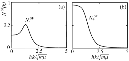
Figure 15: The distribution functions $N_{\sigma}^{\text{SF}}(\mathbf{k})$ for the heavy particles, panel (a), and the light particles, panel (b), in the gapless superfluid phase.

V Fluctuation Effects

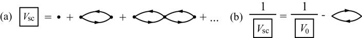
Figure 16: The screened interaction containing an infinite sum of bubble diagrams. Panel (a) shows the perturbative expansion of the screened interaction and panel (b) shows the result of the resummation of this expansion.

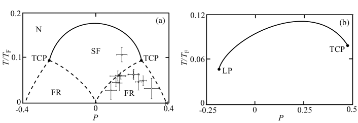
Figure 17: Phase diagrams of strongly interacting Fermi gases, i.e., $1/k_{\text{F}}a=0$, where fluctuation effects have been taken into account. Panel (a) shows the mass-balanced case,i.e., $r=1$. The open squares are data along the phase boundaries from the experiment of Shin et al. Shin . The dashed lines denote the first-order phase transitions, not calculated within our theory and therefore only guides to the eye. However, they include the correct critical polarization at zero temperature, denoted by a cross, known from Monte Carlo calculations Lobo . To calculate the first-order phase transition lines more accurately with fluctuation effects taken into account other methods are needed Diederix . Panel (b) shows the phase diagram for the ⁶Li-⁴⁰K mixture, where $r=6.7$. For both mixtures the critical temperatures are lowered by taking fluctuation effects into account, compare Fig. 7a and Fig. 8a.

As argued before, mean-field theory only leads to a qualitative description of the phase transitions that occur in an imbalanced Fermi gas with unitarity-limited interactions. To achieve also a quantitative description, we have to take fluctuation effects into account. From renormalization-group calculations Koos , we know that especially selfenergy effects and the screening of the interaction by particle-hole fluctuations are important in the unitarity limit. The corresponding corrections result in quantitative agreement with experiments in the mass-balanced case Koos , and give rise to more accurate predictions for upcoming experiments with the very promising ⁶Li-⁴⁰K mixture prl .

As explained in Refs. Diederix ; prl , a convenient way to take selfenergy corrections into account is to introduce renormalized chemical potentials $\mu^{\prime}_{\sigma}$ that describe the selfenergy of particles with spin $\sigma$ in a Fermi sea of particles with spin $-\sigma$. This can be achieved by using

$$\mu^{\prime}_{\sigma}=\mu_{\sigma}+c_{\sigma}\frac{\mu^{\prime 2}_{-\sigma}}{\mu^{\prime}_{\sigma}+\mu^{\prime}_{-\sigma}},$$ (30)

where $c_{\sigma}$ is a coefficient that can be determined in the ladder approximation Combescot , but also with the use of renormalization-group calculations Koos or Monte Carlo calculations Carlson . For the mass-balanced case, we use $c_{\pm}=0.6$, while for the ⁶Li-⁴⁰K mixture we use $c_{+}=2.3$ and $c_{-}=0.36$ to incorporate the Monte Carlo results. The substitution of these renormalized chemical potentials $\mu^{\prime}_{\sigma}(\mu_{\sigma})$ in the mean-field thermodynamic potential $\omega_{\text{L}}(\Delta;\mu^{\prime}_{\sigma})$ results in the following equation for the densities

$$n_{\sigma}=-\left.\frac{\partial\omega_{\text{L}}(\Delta;\mu^{\prime}_{\sigma})}{\partial\mu_{\sigma}}\right|_{\Delta=\langle\Delta\rangle}.$$ (31)

In Ref. prl , an accurate comparison between the use of renormalized chemical potentials and Monte Carlo calculations was made at zero temperatures, leading to excellent agreement. Note that in the superfluid state Eq. (30) overestimates the effects of the interactions on the renormalization of the chemical potentials and another correction proportional to $\Delta^{2}$ has to be subtracted in the right-hand side of Eq. (30) Diederix .

Fluctuations do not only affect the selfenergies of the fermions in the normal state. There is another effect of particle-hole fluctuations that affects the transition to the superfluid state. Namely, there is a change in the coefficient $\alpha$ due to screening of the interspecies interaction, which is also called the Gor’kov correction. We can take the screening into account by considering an effective two-body interaction that includes the so-called random-phase approximation (RPA) bubble sum. This procedure is diagrammatically represented in Fig. 16. The inclusion of the infinite geometric series of bubble diagrams leads at zero external momentum and frequency to

$$\frac{1}{V_{\rm sc}}=\frac{1}{V_{0}}-\hbar\Pi({\bf 0},0),$$ (32)

where $\hbar\Pi({\bf 0},0)$ is the amplitude of the bubble diagram. In Appendix B, it is shown that this amplitude is given by

$$\hbar\Pi({\bf 0},0) = \int\frac{d{\bf k^{\prime}}}{(2\pi)^{3}}\frac{N_{+}({\bf k^{\prime}})-N_{-}({\bf k^{\prime}})}{2h^{\prime}-\epsilon_{+}({\bf k^{\prime}})+\epsilon_{-}({\bf k^{\prime}})},$$ (33)

where we use renormalized chemical potentials to also include the fermionic selfenergy effects. Using the screened interaction of Eq. (32) in Eq. (4), we obtain a screened two-body transition matrix $T^{\rm 2B}_{\rm sc}(0)$, which consequently enters the expression for the quadratic coefficient in Eq. (19). When the quadratic coefficient including screening becomes zero, a second-order transition can occur, so that the critical condition now becomes

$$\alpha_{\rm sc}(T_{\rm c},\mu_{\sigma}^{\prime})=\alpha(T_{\rm c},\mu_{\sigma}^{\prime})+\hbar\Pi({\bf 0},0)=0.$$ (34)

The new critical condition that includes both screening and fermionic selfenergy effects typically reduces the obtained critical temperatures with a factor of three.

If we apply this procedure to determine the line of second-order phase transitions in the mass-balanced case, we obtain the result in Fig. 17a. In this figure, also the data along the phase boundaries from the experiment of Shin et al. Shin are shown. For the unpolarized Fermi gas, we find $T_{\rm c}=0.18T_{\rm F}$ and $\mu(T_{\rm c})=0.51T_{\rm F}$ prl , which is to be compared with the Monte Carlo results $T_{\rm c}=0.15T_{\rm F}$ and $\mu(T_{c})=0.49T_{\rm F}$ Burovski . Moreover, for the location of the mass-balanced tricritical point we find $k_{\rm B}T_{{\rm c}3}=0.09\varepsilon_{\rm F+}$ and $P_{{\rm c}3}=0.24$ prl , which is rather close to the experimental data Shin . We included the critical polarization at zero temperature known from Monte Carlo calculations Lobo , in order to be able to sketch the first-order line and the forbidden region. Other methods are needed to calculate the first-order phase transition more accurately with fluctuation effects taken into account Diederix . In Fig. 17b, we show the line of second-order phase transitions for the ⁶Li-⁴⁰K mixture, when fluctuation effects are included. Compared to the mean-field result of Fig. 14b, the critical temperatures are significantly lower. For the positions of the tricritical point and the Lifshitz point, we use Eq. (20) and Eq. (23), where we again insert the renormalized chemical potentials to include the fermionic selfenergy effects. We then find $k_{\rm B}T_{{\rm c}3}=0.08T_{\text{F}}$ and $P_{{\rm c}3}=0.47$, and $k_{\rm B}T_{\text{L}}=0.05T_{\text{F}}$ and $P_{\text{L}}=-0.18$, respectively prl . It is important to note that although the fluctuations have quantitatively a very large effect, the topology of the phase diagrams remains the same.

VI Discussion and Conclusion

In this paper we considered Fermi mixtures consisting of two different species of fermions, which can both have a population and a mass imbalance. On the mean-field level we calculated the phase diagrams for those Fermi mixtures as a function of temperature and polarization. We calculated the phase diagrams for different mass ratios and for different interaction strengths, where we found that a mass imbalance leads to a phase diagram that is asymmetrical in the polarization. We also considered the possibility of a Lifshitz instability. We found such instabilities in the Fermi mixtures with a mass ration of $r=6.7$ and $r=10$ in the unitarity limit. For a mass-balanced mixture, Lifshitz points occur only in the weakly interacting regime.

By studying the effects of a mass imbalance in more detail we found analytic results for the critical temperature and the change in critical temperature at zero polarization. Furthermore, we investigated what happens to the position of the Lifshitz points and the tricritical points when changing the interaction strength. In the mass-balanced case, we also found a multicritical point for weak interactions. Both for the mass-balanced and the ⁶Li-⁴⁰K Fermi mixtures, we calculated the regions where the superfluid phase is gapless in the unitarity limit, i.e., where the mixtures are in the Sarma phase. These regions were present at nonzero temperatures, and turned out to be quite large.

Finally, to obtain more quantitative results we introduced renormalized chemical potentials that include selfenergy effects to account for the resonant interactions. We also took screening effects on the critical temperature into account. In this way, we obtained a phase diagram for the mass-balanced mixture that agrees well with Monte Carlo calculations and with experiment. And we hope to have obtained a good quantitative description of the phase diagram for the ⁶Li-⁴⁰K mixture, where especially the presence of a Lifshitz point is exciting. Below the Lifshitz point various supersolid states are competitive. This leads to open questions for further research on the interesting possibility of an inhomogeneous superfluid.

VII Acknowledgements

This work is supported by the Stichting voor Fundamenteel Onderzoek der Materie (FOM) and the Nederlandse Organisatie voor Wetenschaplijk Onderzoek (NWO).

Appendix A Derivation of the Mean-Field Thermodynamic Potential

In this Appendix we explicitly derive the mean-field thermodynamic potential in Eq. (13). We start with the microscopic action for an interacting Fermi mixture consisting of fermions present in two hyperfine states. It is given by

$$S[\phi^{*},\phi]=\int_{0}^{\hbar\beta}\text{d}\tau\int\text{d}\mathbf{x}\Big{\{}$$

$$\times\sum_{\sigma=\pm}\phi_{\sigma}^{*}(\mathbf{x},\tau)\left(\hbar\frac{\partial}{\partial\tau}-\frac{\hbar^{2}\nabla^{2}}{2m_{\sigma}}-\mu_{\sigma}\right)\phi_{\sigma}(\mathbf{x},\tau)$$

$$+V_{0}\phi_{+}^{*}(\mathbf{x},\tau)\phi_{-}^{*}(\mathbf{x},\tau)\phi_{-}(\mathbf{x},\tau)\phi_{+}(\mathbf{x},\tau)\Big{\}},$$ (35)

where $V_{0}\,\delta(\mathbf{x-x^{\prime}})$ is the bare point-like interaction associated with the short-range atomic potentials. The last term in this action is a fourth-order term in the fermionic fields. Therefore, the integral over the fermionic fields in the partition function

$$Z=\int\text{d}[\phi^{*}]\text{d}[\phi]\exp\{-S[\phi^{*},\phi]/\hbar\}$$ (36)

cannot be performed analytically. To deal with this fourth-order term we introduce by means of a Hubbard-Stratonovich transformation bosonic pairing fields $\Delta(\mathbf{x},\tau)$, which are on average related to the fermionic fields $\phi_{\sigma}(\mathbf{x},\tau)$ as in Eq. (16). The Hubbard- Stratonovich transformation is performed by inserting into the partition function the following identity

$$1=\int\text{d}[\Delta^{*}]\text{d}[\Delta]e^{(\Delta-\phi_{+}\phi_{-}V_{0}|V_{0}^{-1}|\Delta^{*}-V_{0}\phi^{*}_{-}\phi_{+}^{*})/\hbar},$$ (37)

where the inner product in the exponent is a short hand notation for

$$\noindent\int_{0}^{\hbar\beta}\text{d}\tau\int\text{d}\mathbf{x} (\Delta^{*}(\mathbf{x},\tau)-\phi^{*}_{+}(\mathbf{x},\tau)\phi_{-}^{*}(\mathbf{x},\tau)V_{0})$$

$$V_{0}^{-1}(\Delta(\mathbf{x},\tau)-V_{0}\phi_{-}(\mathbf{x},\tau)\phi_{+}(\mathbf{x},\tau)).$$ (38)

Inserting Eq. (37) into Eq. (36) leaves us with an action $S[\Delta^{*},\Delta,\phi^{*},\phi]$ which depends only quadratically on the fermionic fields $\phi_{\sigma}(\mathbf{x},\tau)$. It is given by

$$S[\Delta^{*},\Delta,\phi^{*},\phi]=-\int_{0}^{\hbar\beta}\text{d}\tau\int\text{d}\mathbf{x}\Bigg{\{}\frac{|\Delta(\mathbf{x},\tau)|^{2}}{V_{0}}$$

$$-\hbar\sum_{\sigma=\pm}\int_{0}^{\hbar\beta}\text{d}\tau^{\prime}\int\text{d}\mathbf{x^{\prime}}\phi^{*}_{\sigma}(\mathbf{x},\tau)G_{0;\sigma}^{-1}(\mathbf{x},\tau;\mathbf{x^{\prime}},\tau^{\prime})\phi_{\sigma}(\mathbf{x^{\prime}},\tau^{\prime})$$

$$+\phi_{+}^{*}(\mathbf{x},\tau)\phi_{-}^{*}(\mathbf{x},\tau)\Delta(\mathbf{x},\tau)+\Delta^{*}(\mathbf{x},\tau)\phi_{-}(\mathbf{x},\tau)\phi_{+}(\mathbf{x},\tau)\Bigg{\}}.$$ (39)

The noninteracting Green’s function is given by

$$G_{0;\sigma}^{-1}(\mathbf{x},\tau;\mathbf{x^{\prime}},\tau^{\prime})$$

$$\hskip 5.69054pt=\frac{1}{\hbar}\left\{\hbar\frac{\partial}{\partial\tau}-\frac{\hbar^{2}\nabla^{2}}{2m_{\sigma}}-\mu_{\sigma}\right\}\delta(\mathbf{x-x^{\prime}})\delta(\tau-\tau^{\prime}).$$ (40)

Note that by performing the Hubbard-Stratonovich transformation we have introduced the order parameter $\Delta(\mathbf{x},\tau)$ in an exact manner into the many-body theory. If we now integrate out the fermionic fields we will be left with an effective action $S^{\text{eff}}[\Delta^{*},\Delta]$, which is directly related to the Landau free energy. If we apply mean-field theory we assume that the bosonic fields are position and time independent, i.e., $\Delta(\mathbf{x},\tau)=\Delta$. In order to integrate out the fermionic fields, we need to diagonalize the action. First, Fourier transforming the above action and then writing it in a more compact way using matrix multiplication yields

$$S[\Delta^{*},\Delta,\phi^{*},\phi]=-\hbar\beta V\frac{|\Delta|^{2}}{V_{0}}-\hbar\beta\sum_{\mathbf{k}}(\varepsilon_{-}(\mathbf{k})-\mu_{-})$$

$$-\hbar\sum_{\mathbf{k},n}\left[\phi_{n,+}^{*}(\mathbf{k}),\phi_{-n,-}(\mathbf{-k})\right]\mathbf{G}^{-1}_{\Delta}(\mathbf{k},\text{i}\omega_{n})\left[\phi_{n,+}(\mathbf{k})\atop{\phi_{-n,-}^{*}(\mathbf{-k})}\right],$$ (41)

where $V$ is the volume. In the above expression

$$-\hbar\mathbf{G}_{\Delta}^{-1}(\mathbf{k},\text{i}\omega_{n})=$$

$$\left[\begin{array}[]{cc}-\text{i}\hbar\omega_{n}+\varepsilon_{+}(\mathbf{k})-\mu_{+}&\Delta\\ \Delta^{*}&-(\text{i}\hbar\omega_{n}+\varepsilon_{-}(\mathbf{k})-\mu_{-})\end{array}\right],$$ (44)

where $\omega_{n}$ are the odd Matsubara frequencies. By writing the action in matrix form, we have interchanged the fermionic fields $\phi_{-}$ and $\phi_{-}^{*}$ and thereby we have picked up a constant term, namely the sum $\Sigma_{\mathbf{k}}(\varepsilon_{-}(\mathbf{k})-\mu_{-})$ in the first line of Eq. (41). We can now diagonalize this action by means of a Bogoliubov transformation. This transformation consists of unitarily transforming the atomic fields $\phi_{n,\sigma}(\mathbf{k})$ to the quasiparticle fields $\psi_{n,\sigma}(\mathbf{k})$

$$\left[\psi_{n,+}(\mathbf{k})\atop{\psi_{-n,-}^{*}(\mathbf{-k})}\right]=\left[\begin{array}[]{cc}u(\mathbf{k})&-v(\mathbf{k})\\ v^{*}(\mathbf{k})&u^{*}(\mathbf{k})\end{array}\right]\cdot\left[\phi_{n,+}(\mathbf{k})\atop{\phi_{-n,-}^{*}(\mathbf{-k})}\right],$$ (47)

where this transformation is unitary if

$$|u(\mathbf{k})|^{2}+|v(\mathbf{k})|^{2}=1.$$ (48)

The coefficients of this transformation can be found by demanding the off-diagonal matrix elements to be zero. The action in terms of the fields $\psi_{n,\sigma}(\mathbf{k})$ then reads

$$S[\Delta^{*},\Delta,\psi^{*},\psi]=-\hbar\beta V\frac{|\Delta|^{2}}{V_{0}}$$

$$-\hbar\beta\sum_{\mathbf{k}}\big{(}\varepsilon(\mathbf{k})-\mu-\hbar\omega(\mathbf{k})\big{)}$$

$$+\sum_{\mathbf{k},n}\left[(-\text{i}\hbar\omega_{n}+\hbar\omega_{+}(\mathbf{k}))\psi_{n,+}^{*}(\mathbf{k})\psi_{n,+}(\mathbf{k})\right.$$

$$\left.+(-\text{i}\hbar\omega_{n}+\hbar\omega_{-}(\mathbf{k}))\psi_{n,-}^{*}(\mathbf{k})\psi_{n,-}(\mathbf{k})\right],$$ (49)

where the extra term $\hbar\omega_{+}(\mathbf{k})$ inside the first sum again comes from interchanging fermionic fields. The mean-field partition function reads after performing the Hubbard-Stratonovich transformation and the Bogoliubov transformation

$$Z =\int\text{d}[\psi^{*}]\text{d}[\psi]\exp\{-S[\Delta^{*},\Delta,\psi^{*},\psi]/\hbar\}$$

$$=\exp\Big{\{}\beta V\frac{|\Delta|^{2}}{V_{0}}+\text{Tr}[\log(-\mathbf{G}^{-1})]\Big{\}}$$

$$=\exp\{-S^{\text{eff}}[\Delta^{*},\Delta]/\hbar\}.$$ (50)

where $\mathbf{G}^{-1}$ is

$$-\hbar\mathbf{G}^{-1}=\left(\begin{array}[]{cc}\text{i}\hbar\omega_{n}-\hbar\omega_{+}(\mathbf{k})&0\\ 0&\text{i}\hbar\omega_{n}-\hbar\omega_{-}(\mathbf{k})\end{array}\right).$$ (51)

The interaction $V_{0}$ in the effective action can be eliminated in favor of the two-body transition matrix using Eq. (4). It is straightforward to calculate the mean-field thermodynamic potential from the effective action, which we find to be

$$\omega_{L}(|\Delta|)=-\frac{1}{\beta V}\log Z=$$

$$-\frac{|\Delta|^{2}}{T^{\text{2B}}(0)}+\int\frac{\text{d}\mathbf{k}}{(2\pi)^{3}}\Big{\{}\varepsilon(\mathbf{k})-\mu-\hbar\omega(\mathbf{k})$$

$$+\frac{|\Delta|^{2}}{2\varepsilon(\mathbf{k})}-\frac{1}{\beta}\sum_{\sigma=\pm}\log\left(1+e^{-\beta\hbar\omega_{\sigma}(\mathbf{k})}\right)\Big{\}},$$ (52)

where to obtain this thermodynamic potential the sum over the Matsubara frequencies was performed using the following identity

$$\sum_{n}\log(\beta(-\text{i}\hbar\omega_{n}+\varepsilon))=\log\left(1+e^{-\beta\varepsilon}\right),$$ (53)

which can be derived using contour integration.

Appendix B Feynman Diagrams

To determine the critical temperature at which a phase transition will take place we can, as mentioned in Section II, either calculate coefficients from the thermodynamic potential by deriving it with respect to $|\Delta|$ or we can use Feynman diagrams. We present the latter scheme in some detail here.

From the action in Eq. (39) we can determine the propagator for the fermionic fields and the vertices for the interactions between the fermions and the bosons. Namely the propagator in momentum space is

$$G_{0,\sigma}(\mathbf{k},\text{i}\omega_{n})=\frac{-\hbar}{-\text{i}\hbar\omega_{n}+(\varepsilon_{\sigma}(\mathbf{k})-\mu_{\sigma})}.$$ (54)

This propagator is in the Feynman diagrams in Figs. 5a and 5b represented by a straight line, where the plus (minus) indicates a light (heavy) particle. The interaction vertex is proportional to $\delta(\mathbf{k_{1}+k_{2}+k_{3}})\delta_{n,n^{\prime},n^{\prime\prime}}$, where $\mathbf{k}_{i}$ are the momenta and $n$ determine the frequencies of the incoming and outgoing particles. This represents nothing but conservation of momentum and energy. In the diagrams in Figs. 5a and 5b the vertices are the points where three propagators meet.

In order to determine the Lifshitz point we need an expression for the ladder diagram with nonzero external momenta.

$$\frac{1}{\hbar\beta}\sum_{n}\int\frac{\text{d}\mathbf{k}}{(2\pi)^{3}}G_{0,+}(\mathbf{q}-\mathbf{k},-\text{i}\omega_{n})G_{0,-}(\mathbf{k},\text{i}\omega_{n})$$

$$=\frac{1}{\hbar\beta}\sum_{n}\int\frac{\text{d}\mathbf{k}}{(2\pi)^{3}}\frac{-\hbar}{\text{i}\omega_{n}\hbar+(\varepsilon_{+}(\mathbf{q-k})-\mu_{+})}$$

$$\times\frac{-\hbar}{-\text{i}\omega_{n}\hbar+(\varepsilon_{-}(\mathbf{k})-\mu_{-})}.$$ (55)

We can split the fractions and then perform the summation over the Matsubara frequencies. This results in

$$\int\frac{\text{d}\mathbf{k}}{(2\pi)^{3}}\frac{N_{+}(\mathbf{q-k})+N_{-}(\mathbf{k})-1}{\varepsilon_{+}(\mathbf{q-k})+\varepsilon_{-}(\mathbf{k})-2\mu}.$$

If we want to obtain the full expression for the quadratic part, we have to add the terms proportional to $|\Delta|^{2}$ from the effective action. By doing so we obtain $\alpha(\mathbf{q})$ in Eq. (21). In the same way the diagrams can be calculated needed for $\alpha$ in Eq. (19) and for $\beta$ in Eq. (20).

When we include fluctuation effects, we also take the screening of the interaction by the particle-hole fluctuations into account. We do so by replacing the bare interaction potential $V_{0}$ by a screened interaction potential $V_{\text{sc}}$ containing the infinite sum of so-called RPA bubble diagrams, see Fig. 16. The sum over all the bubble diagrams in Fig. 16 is a geometric series. Using this, we find the result for the screened interaction Eq. (32). Thus, to find the screened interaction, we have to calculate the amplitude of the bubble diagram. The bubble diagram consists of two fermionic propagators with momentum and energy going in opposite directions through the diagram. The amplitude is given by

$$\frac{1}{\hbar\beta}\sum_{n}\int\frac{\text{d}\mathbf{k}}{(2\pi)^{3}} \frac{-\hbar}{-\text{i}\hbar\omega_{n}+\varepsilon_{+}(\mathbf{k})-\mu_{+}}$$

$$\times\frac{-\hbar}{-\text{i}\hbar\omega_{n}+\varepsilon_{-}(\mathbf{k})-\mu_{-}}.$$ (56)

Writing the above expression as the sum of two fractions and then performing the sum over the Matsubara frequencies results in

$$\hbar\Pi(\mathbf{0},0)=\int\frac{\text{d}\mathbf{k}}{(2\pi)^{3}}\frac{N_{+}(\mathbf{k})-N_{-}(\mathbf{k})}{2h-(\varepsilon_{+}(\mathbf{k})-\varepsilon_{-}(\mathbf{k}))}.$$ (57)

References

- (1) M. Greiner, C. A. Regal, D. S. Jin, Nature 426, 537 (2003).
- (2) S. Jochim et al., Science 302, 2101 (2003).
- (3) C. A. Regal, M. Greiner, D. S. Jin, Phys. Rev. Lett. 92, 040403 (2004).
- (4) M. W. Zwierlein et al., Phys. Rev. Lett. 92, 120403 (2004).
- (5) J. Kinast et al., Phys. Rev. Lett. 92, 150402 (2004).
- (6) M. Bartenstein et al., Phys. Rev. Lett. 92, 203201 (2004).
- (7) T. Bourdel et al., Phys. Rev. Lett. 93, 050401 (2004).
- (8) G. B. Partridge et al., Phys. Rev. Lett. 95, 020404 (2005).
- (9) M. W. Zwierlein et al., Science 311, 492 (2006).
- (10) G. B. Partridge et al., Science 311, 503 (2006).
- (11) Y. Shin et al., Nature 451, 689 (2008).
- (12) K. B. Gubbels, M. W. J. Romans, H. T. C. Stoof, Phys. Rev. Lett. 97, 573 210402 (2006).
- (13) J. M. Diederix, K. B. Gubbels, H. T. C. Stoof, arXiv:0907.0127v2 (2009).
- (14) D. Bailin and A. Love, Phys. Rept. 107, 325 (1984).
- (15) R. Casalbuoni and G. Nardulli, Rev. Mod. Phys. 76, 263 (2004).
- (16) K. B. Gubbels, J. E. Baarsma, H. T. C. Stoof, Phys. Rev. Lett. 103, 195301 583 (2009).
- (17) A. I. Larkin and Y. N. Ovchinnikov, Zh. Eksp. Teor. Fiz. 47, 1136 (1964).
- (18) P. Fulde and R. A. Ferrell, Phys. Rev. 135, A550 (1964).
- (19) A. Bulgac and M. McNeil Forbes, Phys. Rev. Lett. 101, 215301 (2008).
- (20) Y. Liao et al., arXiv:0912.0092 (2009).
- (21) C. Mora and R. Combescot, Phys. Rev. B 71, 214504 (2005).
- (22) N. Yoshida and S.-K. Yip, Phys. Rev. A 75, 063601 (2007).
- (23) E. Wille et al, Phys. Rev. Lett. 100, 053201 (2008).
- (24) A.-C. Voigt et al, Phys. Rev. Lett. 102, 020405 (2009).
- (25) M. M. Parish et al, Phys. Rev. Lett. 98 160402 (2007).
- (26) L. P. Gor’kov and T. K. Melik-Barkhudarov, Sov. Phys. JETP 13, 1018 (1961).
- (27) K. B. Gubbels and H. T. C. Stoof, Phys. Rev. Lett. 100, 140407 (2008).
- (28) E. Burovski et al., Phys. Rev. Lett. 96, 160402 (2006).
- (29) R. A. Duine and H. T. C. Stoof, Phys. Rep. 396,115 (2004).
- (30) M. W. J. Romans, H. T. C. Stoof, Phys. Rev. Lett. 95, 260407 (2005).
- (31) J. W. Negele, H. Orland, Quantum Many-Particle Systems (Westview Press, Boulder, 1998).
- (32) H. T. C. Stoof, K. B. Gubbels, D. B. M. Dickerscheid, Ultracold Quantum Fields (Springer, Dordrecht, 2009).
- (33) P. M. Chaikin and T. C. Lubensky, Principles of Condensed Matter Physics (Cambridge University Press, Cambridge, 1995).
- (34) M. Iskin and C. A. R. Sá de Melo, Phys. Rev. A 77, 013625 (2008).
- (35) A. L. Fetter, J. D. Walecka, Quantum Theory of Many-Particle Systems (McGraw-Hill, New York, 1971).
- (36) G. Sarma, J. Phys. Chem. Solids 24, 1029 (1963).
- (37) H. Kleinert, Forts. Phys. 26, 565 (1978).
- (38) T. Paananen, P. Törmä, J.-P. Martikainen, Phys. Rev. A 75, 023622 (2007).
- (39) M. M. Parish et al, Nature Physics 3, 124 (2007).
- (40) A. I. Buzdin and H. Kachkachi, Phys. Lett. A 225, 341 (1997)
- (41) C. A. Sá de Melo et al., Phys. Rev. Lett. 71, 3202 (1993).
- (42) R. Combescot et al., Phys. Rev. Lett. 98, 180402 (2007).
- (43) C. Lobo et al., Phys. Rev. Lett. 97, 200403 (2006).
- (44) A. Gezerlis et al., arXiv:0901.3105 (2009).