Simulation of Flow of Mixtures Through Anisotropic Porous Media using a Lattice Boltzmann Model

Abstract

We propose a description for transient penetration simulations of miscible and immiscible fluid mixtures into anisotropic porous media, using the lattice Boltzmann (LB) method. Our model incorporates hydrodynamic flow, diffusion, surface tension, and the possibility for global and local viscosity variations to consider various types of hardening fluids. The miscible mixture consists of two fluids, one governed by the hydrodynamic equations and one by diffusion equations. We validate our model on standard problems like Poiseuille flow, the collision of a drop with an impermeable, hydrophobic interface and the deformation of the fluid due to surface tension forces. To demonstrate the applicability to complex geometries, we simulate the invasion process of mixtures into wood spruce samples.

1 Introduction

Fluid invasion and flow in porous media are ubiquitous phenomena in nature and technology. In principle, studies on porous media can be classified by three length scales: the pore scale, the representative volume element (RVE) scale, and the domain scale handbook . Studies on the pore scale directly model the pore space geometry and the fluid hydrodynamics hajoe . The intermediate sized RVE is the minimum volume required to characterize the flow through the medium. Most systems are studied on the RVE scale, using semi-empirical theories. This is necessary due to complex pore space geometries. Typical examples are the Darcy, the Brinkman-extended Darcy, and the Forchheimer - extended Darcy models handbook . The flow in porous media can also be modeled via generalized Navier-Stokes equations Tien ; Hsu ; Nith , including all necessary terms in one momentum conservation equation. Unfortunately in the majority of cases, the analytical solution becomes very difficult and is even complicated for anisotropic, structured porous media like wood. Therefore, one depends on numerical methods in this field. The fluid itself can be quite complicated as well. It can be a miscible or immiscible mixture of different species, its viscosity can change locally due to internal chemical reactions like hardening and can depend on shear velocities in the case of Non-Newtonian fluids. Examples are adhesive penetration at wood junctures or the impregnation or sealing of concrete for protective reasons. A practical model approach for these phenomena is hydrodynamic dispersion jacobbear that treats one fluid, e.g. a solvent, by the hydrodynamic theory and the others, e.g. solutes, by diffusion equations. For complicated anisotropic porous media and fluids, coupling the diffusion with the generalized Navier-Stokes equations makes analytical solutions quite difficult. However, numerical solutions can be found. The motivation for the present work is adhesive penetration in wood.

Wood constructions depend on good adhesive bondings, that are the result of a gluing process, where hardening liquids are pressed into a porous, anisotropic micro structure. Depending on the penetration and adhesive hardening characteristics, preferrable interface morphologies can be obtained kamke-lee-2007 . The penetration is dominated by the strong anisotropy of the permeability tensor and the viscosity evolution of the adhesive. Due to the difficulty of the problem, penetration simulations with classical continuum mechanics are hardly feasible.

Over the last two decades, lattice Boltzmann (LB) methods developed to be an alternative to the simulation of partial differential equations (PDEs). Originally LB methods were developed as discrete realizations of kinetic models for fluids n5 ; n38 . Extensions allow for the simulation of diffusion flekkoy , waves n101 ; chop , magnetohydrodynamics n39 ; n6 ; nmiller , quantum mechanics s93 , and multiphase flows ReisPhillips ; Mlatva ; Daryl ; jonathanchin ; Xiaowen ; andrewk . Tölke et. al. made a first study on binary flows in porous media jonasmanfred . The authors consider two immiscible fluids that evolve inside a pore scale system by the Navier-Stokes equations with interaction terms. LB models for incompressible flows through porous media on the RVE scale were first addressed by Guo et. al. preGuo , who proposed a 2D model including a nonlinear Forchheimer term, that can be used for isotropic, heterogeneous porous media.

We introduce a 3D LB model that recovers the generalized Navier-Stokes equations in anisotropic porous media, extended by the diffusion equation for the solute concentration in fluid mixtures. Consequently viscosity changes appear, that can be superimposed by local hardening. Additionally we incorporate the free surface technique freesurface to allow for immiscible fluids. In this paper, Sec. 2 first describes some LB fundamentals and the numerical model details for fluid and diffusive particles. Sec. 3 shows a brief description of the free surface technique while Sec. 4 addresses the implementation of the algorithm and Sec. 5 demonstrates the validity of our model and its application to diverse physical systems.

2 3D Lattice-Boltzmann Model for Anisotropic Porous Media

We begin with the generalized Navier-Stokes equations for low Reynolds numbers with mass conservation

$${}\frac{\partial\rho}{\partial t}+\nabla\cdot(\rho\vec{V})=0\quad,$$ (1)

and momentum conservation,

$${}\frac{\partial\vec{V}}{\partial t}+(\vec{V}\cdot\nabla)\biggl{(}\frac{\vec{V}}{\epsilon}\biggr{)}= -\frac{\nabla(\epsilon P)}{\rho}+\nu_{e}\nabla^{2}\vec{V}+\epsilon\vec{G}$$

$$-\epsilon\nu\mathsf{K}^{-1}\cdot\vec{V}-\frac{\epsilon}{\rho}\nabla\cdot\mathsf{S}\quad,$$

with the fluid density $\rho$ and viscosity $\nu$, the volume-averaged velocity and pressure $\vec{V}$ and $P$. $\epsilon$ denotes the porosity of the medium, $\mathsf{K}$ the permeability tensor that can be anisotropic, and $\vec{G}$ represents an external force field. The quantity $\nu_{e}$ is named the effective viscosity which is not expected to be the same as the viscosity of the fluid due to the effects of tortuosity and the dispersion of viscous diffusion flux handbook . The surface tension tensor $\mathsf{S}$ can be expressed by

$${\bf S}=\frac{2A\tau}{9|\vec{F}|}\cdot\left(\begin{array}[]{ccc}-F^{2}_{y}-F^{2}_{z}&F_{x}F_{y}&F_{x}F_{z}\\ F_{x}F_{y}&-F^{2}_{x}-F^{2}_{z}&F_{y}F_{z}\\ F_{z}F_{x}&F_{z}F_{y}&-F^{2}_{x}-F^{2}_{y}\end{array}\right)\quad,$$ (3)

with the color gradient $\vec{F}$$=$$\nabla\rho$, a parameter $A$ that fixes the strength of the surface tension, and the characteristic relaxation time $\tau$, that is fixed by the effective viscosity $\nu_{e}$$=$$\frac{1}{3}(\tau-\frac{1}{2})$ surfacetension . Most of these quantities are related to each other like the pressure $P$$=$$\rho c^{2}_{s}/\epsilon$ depending on the speed of sound of the fluid $c_{s}$. In the following we demonstrate how Navier-Stokes equations are reproduced by LB methods, and how extensions like external forces, Darcy flow, and surface tension can be added to the framework. Diffusion however is treated differently and explained separately.

2.1 Model Description for the Generalized Navier-Stokes Equations

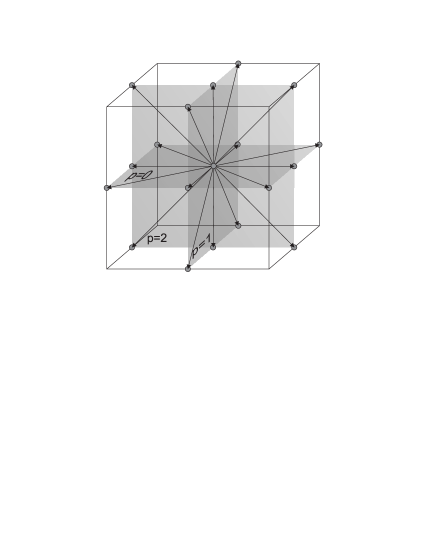
Figure 1: Cubic lattice D3Q19 discretization of the fluid velocity. The arrows represent the velocity vectors $\vec{v}_{i}^{p}$, where $p$ indicates the plane of location. Note that by including the rest vector located in the center of the cell, totally 19 directions are defined.

The basic principle of LB is that Navier-Stokes equations are not solved directly on a grid of cells, but via a strongly simplified particle micro dynamics with discrete Boltzmann equations and collision rules such as Bhatnagar-Gross-Krook (BGK) n13 . The two ingredients particle streaming and collision are calculated along a certain number of fixed orientations (19 in our case as illustrated in Fig.1) in each cubic cell with lattice constant $\delta x$$=$$\delta t$. The velocity vectors are denoted by $\vec{v}_{i}^{p}$, where $i$$=$$1...6$, indicates their orientation and $p$$=$$0,1,2$ their reference plane (see Fig.1). Each velocity vector $\vec{v}_{i}^{p}$ comes along with one assigned distribution function $f_{i}^{p}$. The density $\rho$ in a cell is the sum over its distribution functions

$${}\rho=\sum_{i=1}^{6}\sum_{p=0}^{2}f_{i}^{p}\quad.$$ (4)

We obtain continuum properties for $\vec{V}$ and $\vec{F}$ via

$${}\rho\vec{V}=\sum_{i=1}^{6}\sum_{p=0}^{2}f_{i}^{p}\vec{v}_{i}^{p}\quad,\qquad\vec{F}=\sum_{i=1}^{6}\sum_{p=0}^{2}\rho(\vec{x}+\vec{v}_{i}^{p})\vec{v}_{i}^{p}\quad.$$ (5)

In order to include the influence of the porous media, of external forces, and of surface tension on the momentum equation (Eq. 2), we need to include additional force terms in the LB model. Following the work of Guo et.al. n30 , we add two force terms $T_{i}^{p}$ and $T_{0}$ to each of our 19 directions, including the rest vector in the cell’s center:

$${}f_{i}^{p}(\vec{x}+\vec{v}_{i}^{p},t+1)-f_{i}^{p}(\vec{x},t) =\Omega_{i}^{p}(\vec{x},t)+T_{i}^{p},$$ (6)

$$f_{0}(\vec{x},t+1)-f_{0}(\vec{x},t) =\Omega_{0}(\vec{x},t)+T_{0}\quad.$$

The second ingredient of LB are the BGK collision terms $\Omega_{i}^{p}$ and $\Omega_{0}$ n13

$$\Omega_{i}^{p} =-\frac{1}{\tau}(f_{i}^{p}(\vec{x},t)-f_{i}^{p,\rm eq}(\vec{x},t))\quad,$$ (7)

$$\Omega_{0} =-\frac{1}{\tau}(f_{0}(\vec{x},t)-f_{0}^{\rm eq}(\vec{x},t))\quad.$$

The subscript ^eq denotes the equilibrium states for the distribution functions, which we must find such that the model reproduces correctly the hydrodynamic equations. $\tau$ denotes again the relaxation time from Eq. 3. The force terms $T_{i}^{p}$ and $T_{0}$ are given by n30 :

$$T_{i}^{p} =\biggl{(}1-\frac{1}{2\tau}\biggr{)}\biggl{(}3(\vec{v}_{i}^{p}\cdot\vec{F}^{ext})+\frac{9}{\epsilon}(\vec{v}_{i}^{p}\cdot\vec{V^{\prime}})(\vec{v}_{i}^{p}\cdot\vec{F}^{ext})$$

$$-\frac{3}{\epsilon}(\vec{V^{\prime}}\cdot\vec{F}^{ext})\biggr{)}\quad,$$

$$T_{0}=\biggl{(}1-\frac{1}{2\tau}\biggr{)}\biggl{(}-\frac{3}{\epsilon}\vec{V^{\prime}}\cdot\vec{F}^{ext}\biggr{)}\quad,$$

with the external force

$$\vec{F}^{ext}=-\epsilon\nu\mathsf{K}^{-1}\cdot\vec{V^{\prime}}+\epsilon\vec{G}$$ (9)

in our case. Due to the external forces, the velocity $\vec{V}$ needs to be corrected to obtain $\vec{V^{\prime}}$ by

$$\vec{V^{\prime}}=\vec{V}+\frac{1}{2}\vec{F}^{ext}\quad.$$ (10)

Unfortunately $\vec{F}^{ext}$ depends on $\vec{V^{\prime}}$. Then we insert Eq. 9 into Eq. 10 and obtain

$${}\vec{V^{\prime}}=\mathsf{\Lambda}^{-1}\cdot\biggl{(}\vec{V}+\frac{1}{2}\vec{G}\biggr{)}\quad,$$ (11)

where we define $\mathsf{\Lambda}$$=$$\mathsf{I}+\frac{\epsilon\nu}{2}\mathsf{K}^{-1}$ with the identity matrix $\mathsf{I}$.

We finally write down the equilibrium functions for our system:

$${}f_{i}^{p,\rm eq}(\vec{x},t) =w_{i}\rho\biggl{[}1+3(\vec{v}_{i}^{p}\cdot\vec{V^{\prime}})+\frac{9}{2\epsilon}(\vec{v}_{i}^{p}\cdot\vec{V^{\prime}})^{2}$$

$$-\frac{3}{2\epsilon}\vec{V^{\prime}}^{2}+\frac{A\epsilon\tau}{\rho}\biggr{(}\frac{(\vec{v}_{i}^{p}\cdot\vec{F})^{2}}{|\vec{F}|}-|\vec{F}|\biggl{)}\biggl{]}\quad,$$

$${}f_{0}^{\rm eq}(\vec{x},t)=w_{0}\rho\biggl{[}1-\frac{3}{2\epsilon}\vec{V^{\prime}}^{2}\biggr{]}+A\epsilon\tau w_{0}|\vec{F}|\quad,$$ (13)

with the known weights $w_{0}=1/3$, $w_{1,2,3,4}=1/36$, and $w_{5,6}=1/18$ for the D3Q19 cells weightcitation . The last terms in Eqs. 2.1,13 represent the surface tension. In the continuum limit, the surface tension tensor ${\bf S}$ from Eq. 2 is reproduced. Note that it can be shown analytically chapman that this LB BGK model recovers the generalized Navier-Stokes equations Eqs. 1,2 in the isothermal and incompressible limit with surface tension.

2.2 Lattice Boltzmann model for solute diffusion

To consider diffusion in an LB framework, we can either define an additional set of velocity vectors and include their diffusive terms directly into the equilibrium function (Eq. 2.1), or define additional equilibrium distribution functions for the diffusion but work on the same velocity vectors as proposed by Hiorth et. al. difusion on a D2Q9 cell configuration. In this work, the second approach was chosen, to simplify a later extension to various species. We therefore recover the diffusion equation in porous media based on Ref. difusion , but extend it to heterogeneous porous media. Starting from the diffusion equation

$$\frac{\partial C}{\partial t}+\nabla\cdot(C\vec{U})=\nabla\cdot[D\nabla C]\quad,$$ (14)

with the concentration $C$, the diffusivity $D$, and the velocity of the mixture $\vec{U}$, Hiorth et. al. difusion use a D2Q9 cell configuration and define a distribution function $h_{i}$ for each velocity vector. The concentration is calculated via $C$$=$$\sum_{i=1}^{9}h_{i}$ and the equilibrium equations are defined by

$${}h_{i}^{\rm eq}(\vec{x},t)=w_{i}C\biggl{[}1+3(\vec{v}_{i}^{p}\cdot\vec{U})\biggr{]}\quad,\quad h_{0}^{\rm eq}(\vec{x},t)=w_{0}C\quad,$$ (15)

with the weights $w_{0}$$=$$4/9$, $w_{1,2,3,4}$$=$$1/9$, and $w_{5,6,7,8}$$=$$1/36$ difusion . To extend to 3D and to include the porous medium, we propose modified equilibrium distribution functions on a D3Q19 cell configuration (see Fig. 1)

$${}h_{i}^{p,\rm eq}(\vec{x},t)=w_{i}\epsilon C\biggl{[}1+3(\vec{v}_{i}^{p}\cdot\vec{V^{*}})\biggr{]}\quad,\quad h_{0}^{\rm eq}(\vec{x},t)=w_{0}\epsilon C\quad,$$ (16)

where $\vec{V^{*}}$$=$$\vec{V^{\prime}}+D\frac{\nabla\epsilon}{\epsilon}$. With the correct weights $w_{0,i}$ for the D3Q19 cell, we evolve Eq. 16 according to the Boltzmann equation with the BGK collision term $\Omega_{Di}^{p}(\vec{x},t)$ n13 :

$$h_{i}^{p}(\vec{x}+\vec{v}_{i},t+1)-h_{i}^{p}(\vec{x},t)=\Omega_{Di}^{p}(\vec{x},t)\quad,$$ (17)

$$\Omega_{Di}(\vec{x},t)=-\frac{1}{\tau_{D}}(h_{i}^{p}(\vec{x},t)-h_{i}^{p,\rm eq}(\vec{x},t))\quad.$$

Now $\tau_{D}$ defines the relaxation time for the diffusion model with the diffusivity, $D$$=$$\frac{1}{3}(\tau_{D}-\frac{1}{2})$. We can prove via a Chapmann-Enskog expansion that the model reproduces

$$\frac{\partial(\epsilon C)}{\partial t}+\nabla\cdot(\epsilon C\vec{V^{\prime}})=\nabla\cdot[\epsilon D\nabla C]$$ (18)

in the continuum limit.

The full model can now reproduce the generalized Navier-Stokes equations in the continuum limit for anisotropic porous media, including surface tension and the diffusion-advection of the solute. To complete the description of the model, we will briefly summarize the free surface technique freesurface used to describe the movement of fluid with a fluid-gas interface.

3 The Free Surface Technique

If a fluid penetrates an unsaturated porous medium, free surfaces form. To include free surfaces in our LB scheme a free surface technique freesurface is necessary. If a cell is only filled by gas with a negligible density, Eqs. 2.1 and 13 lead to vanishing equilibrium functions and the simulation becomes unstable. This problem can be solved by classifying fluid cells into three types of cells: the liquid cells, totally filled by liquid fluid, the empty cells entirely filled by gas, and the interface cells that contain both fluids: liquid and gas. The purely liquid filled cell were discussed in the previous section, while gas filled cells can be excluded from the further calculation due to the high density ratio between fluid and gas. However the interface cells need further attention.

Interface cells consist partially of liquid and of gas, determined by the fluid fraction $\lambda(\vec{x},t)$ $=m(\vec{x},t)/\rho(\vec{x},t)$ with the mass $m$ of liquid in the cell located in $\vec{x}$ at time $t$. Using a normalized cell volume, the mass for the fluid cell is equal to the density of the liquid, and for gas cells equal to zero. Analogous to Eq. 4, we obtain the macroscopic mass $m(\vec{x},t)$ by summing the mass functions $m_{i}^{p}$ over all directions

$$m(\vec{x},t)=\sum_{i=1}^{6}\sum_{p=0}^{2}m_{i}^{p}\quad.$$ (19)

The mass functions $m_{i}^{p}$ evolve according to

$$m_{i}^{p}(\vec{x},t+1)=m_{i}^{p}(\vec{x},t)+\sum_{i=1}^{6}\sum_{p=0}^{2}\Delta m_{i}^{p}(\vec{x},t+1)\quad,$$ (20)

with

$$\Delta m_{i}^{p}(\vec{x},t+1)=f_{j}^{p}(\vec{x}+\vec{v}_{i}^{p},t)\frac{\lambda(\vec{x}+\vec{v}_{i}^{p},t)+\lambda(\vec{x},t)}{2}$$ (21)

$$-f_{i}^{p}(\vec{x},t)\frac{\lambda(\vec{x}+\vec{v}_{i}^{p},t)+\lambda(\vec{x},t)}{2}\quad,$$

where the index $j$ stands for the vector with opposite direction to the vector with index $i$. The interface cells also have associated distribution functions that evolve via the discrete Boltzmann Eq. 6 identical to those in the fluid cells. These distribution functions are used to calculate the density and the updated fluid fraction $\lambda$.

Nevertheless, we still obtain zero distribution functions in the interface cells from Eq. 6, due to empty neighboring cells. To avoid this problem, we calculate the evolution of distribution functions of interface cells originating from empty neighboring cells with the modified function

$$f_{j}^{p}(\vec{x},t+1)=f_{i}^{p,\rm eq}(\vec{x},t)+f_{j}^{p,\rm eq}(\vec{x},t)-f_{i}^{p}(\vec{x},t)\quad.$$ (22)

During the system evolution, the interface moves, leading to changes in the fluid fraction $\lambda$. If $\lambda$ becomes unity, the cell changes to a liquid cell, while $\lambda\rightarrow 0$ leads to gas or empty cells. To complete the picture all cells neighboring new liquid cells are set to interface cells. To summarize, by classifying cell types and corresponding distribution functions, depending on fluid type, we can capture the evolution of free surfaces. A more detailed description can be found in Ref. freesurface . Finally this technique extends our model to simulations of fluid penetration with gas/liquid interface. Before validation examples are shown, we outline the implementation of the algorithm.

4 Algorithm Implementation

To obtain a transparent, portable simulation code, we implemented it object oriented in C++. The general framework of a simulation is given in Fig. 2.

Figure 2: Computational procedure of the LB simulation of flow of mixtures through anisotropic porous media including free surface and tension effects.

First we set all initial field values like the density $\rho$, the velocity $\vec{V}$, external force field $\vec{F}^{ext}$ (Eqs. 4,5), and the solvent concentration $C$ inside the mixture. To completely define the system, the porosity field, the permeability fields, and relaxation times are set. Also the initial saturation and boundary conditions like periodicity, pressures, flow rate, or impermeability are imposed. We can define three types of cells: fluid, interface and empty, depending on the problem. With these quantities set, we can start calculating the distribution functions $f_{i}^{p},~{}h_{i}^{p}$ from the equilibrium distribution functions $f_{i}^{p,\rm eq}$ and $h_{i}^{p,\rm eq}$ (Eqs. 2.1,13,16). Now, the time step can be incremented and system is ready to evolve (see Fig. 2).

To follow the evolution of the system, first solve the stream to all neighboring cells, stream their mass and calculate the macroscopic variables. Then the color gradient $\vec{F}$ is calculated. Finally, we have to update the type of cells and increment the time to prepare the system for the next time step. These steps are looped over all cells in the system. We stop the simulation, when a stable state is reached.

5 Model Validation and Calculation of the Flow Profile of Adhesives in Wood

To validate our LB model implementation, we simulate systems with known analytical solutions that especially address each term that appears in the generalized Navier-Stokes equations. In particular we simulate Poiseuille flow through isotropic and anisotropic porous media, droplet formation, and fluid surface smoothening. Finally, we show an application for the penetration of hardening mixtures into an anisotropic, heterogeneous porous medium, demonstrating the capability of the model to represent adhesive penetration in complex materials like wood.

5.1 Single Fluid in Homogeneous, Isotropic Porous Media

To show the capability of the model to reproduce the Darcy law in a simple case, we simulate a generalized Poiseuille flow driven by a constant force in an isotropic, homogeneous medium between two infinite plates at distance $L$ (see Fig.3). For this case, we need neither the surface tension tensor nor the free surface technique. Therefore just the force terms from the Darcy law, body force and the viscosity terms on the right hand of Eq. 2 are active.We impose periodic boundary conditions on all velocity vectors and null velocity at $y$$=$$0,L$ of our 3D system. We only consider movements in the $x$-direction, so the velocity has form $\vec{V}$$=$$(V_{x},0,0)$ with boundary values of $V_{x}(x,0)$$=$$V_{x}(x,L)$$=$$0$. The analytical solution of this problem is well known handbook by a Brinkman-extended Darcy equation, and has the form,

$$V_{x}(y)=\frac{GK}{\nu}\left(1-\frac{\cosh[r(y-L/2)]}{\cosh[rL/2]}\right)\quad,$$ (23)

where $r$$=$$\sqrt{\frac{\nu\epsilon}{K\nu_{e}}}$.

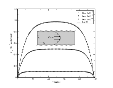
Figure 3: Velocity profile for a generalized Poiseuille flow in a homogeneous, isotropic porous medium for various Darcy numbers. The generalized Poiseuille flow is obtained when the fluid moves through a channel between two walls driven by a constant body force through the porous medium (shaded zone).

We set up a system of $3$$\times$$100$$\times$$1$ cells with porosity $\epsilon=0.3$, relaxation time $\tau=0.6$, density $\rho$$=$$1.0$, and the body force $\vec{G}$$=$$(0.1,0,0)$. The permeability $K$ is fixed by the Darcy number $Da$$=$$K/L^{2}$ to $10^{-3}$, $5$$\times$$10^{-3}$, and $10^{-4}$ respectively. We start with a flat profile and let the system evolve. When the velocity profile reaches a steady state, the simulation is stopped. Comparing the solution to Eq. 23 we find excellent agreement with the theory (see Fig. 3).

5.2 Anisotropic Permeability

In order to validate the model for anisotropic porous media, we study Poiseuille flow like in Sec. 5.1, but with a diagonal permeability tensor $\mathsf{K}$, that was fixed to $\mathsf{K}$ $=$ $10^{-3}\delta_{xx}+10^{-5}\delta_{yy}$.

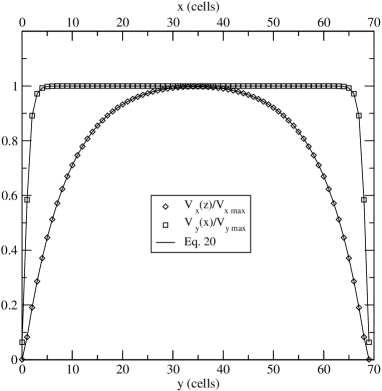
Figure 4: Velocity profiles for an anisotropic porous medium with diagonal permeability tensor. Squares denote the velocity profile of the $x$ component and diamonds represent the simulation with flow in $y$-direction ($v_{x,max}=3\cdot 10^{-3}$, $v_{y,max}=3\cdot 10^{-5}$).

First, we let the fluid move inside the porous medium in $x$-direction like before with $V_{x}(y=0,L)$$=$$0$ at the bottom and top. In a second simulation the fluid moves in $z$-direction with $V_{y}(x=0,L)$$=$$0$ at the vertical boundaries. The velocity profiles can be calculated again by Eq. 23. In the simulation we used an array of $70$$\times$$70$$\times$$1$ cells with the same porosity, relaxation time and density as previously. However the body force is $\vec{G}$$=$$(0.1,0,0)$ for the first case and $\vec{G}$$=$$(0,0.1,0)$ for the second one. We run the simulation until the system reaches a steady state and measure the respective velocity profiles (see Fig. 4). The simulation results show that the model reproduces the Darcy flow in anisotropic porous media accurately.

5.3 Free Surface Model

As condition for a valid implementation of the free surface technique, we have to assure, that our model conserves mass. This can be tested by simulating a freely falling droplet followed by its collision against an impermeable, hydrophobic wall.

The system consists of a grid of $140$$\times$$140$$\times$$1$ cells. Initially a droplet with a radius of $8$ cells is placed in the upper part of the system and an impermeable surface avoids its penetration through the bottom of the simulation zone at $y$$=$$0$. The system parameters are fluid density $\rho=1.0$, relaxation time $\tau$$=$$0.7$, external gravitational force $\vec{G}$$=$$1\cdot 10^{-6}\cdot(0,1,0)$. The impermeable wall is modelled by setting the macroscopic velocity in the respective cells to zero. The force terms from the Darcy law and surface tension are neglected here.

In Fig. 5 we plot the droplet mass as function of time. We can see that the mass is conserved with a small error of less than $1$$\%$. Note also that this error is within the range of common errors that go along with LB simulations. After approximately $10600$ time steps we find an abrupt peak in the total mass due to the collision with the wall. Note that due to numerical reasons, for a short time mass is transferred to the boundary cells that represent the impermeable wall, but is returned in the next time steps, so that the total mass recovers the value previous to the collision. The initial and final configurations after $20000$ time steps are shown in the figure’s inset.

Figure 5: Evolution of the total mass of a falling droplet that crashes against an impermeable, hydrophobic wall. Inset: Snapshots of the droplet at initial time (a) and after $20000$ time steps (b).

5.4 Introduction of the Surface Tension

Mass conservation alone is not sufficient to describe free surfaces, rather surface tension needs to be considered. A correct implementation can be for example tested by simulating the deformation of the fluid from a rectangular to a circular shape. In this spirit we implemented a simulation using an array of $100$$\times$$100$$\times$$1$ cells, with an initially filled, square fluid zone of size $20$$\times$$20$ cells (see Fig. 6). The density and relaxation time are identical to the droplet simulation, and a surface tension parameter $A$$=$$0.001$ was chosen (see Eq. 3). The force terms from the Darcy law and external forces like gravity were switched off for this simulation. The system evolved until a steady state was reached after $10000$ time steps. The final shape of the fluid surface smoothened due to surface tension is seen in Fig. 6.

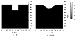
Figure 6: Surface smoothing due to surface tension from the initial shape (a) to the final shape after $10000$ time steps (b). Intensities represent the quantity of fluid in each cell where black means empty cells and white completely filled ones.

Summarizing, we showed that the model can reproduce the theory of single fluids in the case of anisotropic porous media with surface tension effects and external forces. Note that in our case it is only possible to apply the free surface technique to liquids with low Reynold numbers.

5.5 Penetration of Adhesives in Wood

To demonstrate the applicability of our model, we describe the simulation of the penetration of adhesives into wood which is an anisotropic porous medium. The adhesives can be treated like two fluids: a polymer (solute) and a solvent, e.g. water. The polymer dynamics is governed by the diffusion equation and the solvent by the generalized Navier-Stokes equations. To consider hardening effects in the adhesive, we have to consider a local change in time of the viscosity due to the change of concentration. An additional difficulty is the description of the anisotropic porous medium wood. We need to obtain the permeability tensor of wood and to implement a law for the dependency of the viscosity with the concentration and time.

Wood properties:

In wood, the orthotropic permeability tensor and density is a local property, depending mainly on year ring geometry, orientation, and position inside the year ring. Following Refs. wittel ; Bouriaud an empirical expression of the wood density of the type

$$\rho(x)=\rho_{0}[1+2ax^{b}\exp(-cx)]\quad,$$ (24)

with the parameters $a$, $b$, $c$, the position $x$, and the minimum density $\rho_{0}$ can be made with parameters depending on the type of wood. For spruce we can take values of $\rho_{0}$$=$$310$kg/m³, $a$$=$$\frac{24}{\Delta}$, $b$$=$$0.8$, and $c$$=$$\frac{9.6}{\Delta}$, where $\Delta$$=$$2.9$mm is the year ring width wittel . To represent several parallel year rings, we use a periodic function of the form of Eq. 24 with periodic $\Delta$. Since wood consists of cell walls and lumen, we can estimate the porosity from the density by

$$\epsilon(x)=1-\frac{\rho(x)}{\rho_{max}}\quad,$$ (25)

where $\rho_{max}$ is the density of cell walls. Permeability and porosity are related in the scalar case by handbook

$$K=\frac{\epsilon^{3}}{n(1-\epsilon)^{2}}D_{p}^{2}\quad,$$ (26)

with the characteristic pore size $D_{p}$ and a constant $n$ that parametrizes the microscopic geometry of the material taken as $n$$=$$150$ in our case. In wood, the pore size $D_{p}$ must also depend on the wood density, and we propose as a first approximation the relation

$$D_{p}(x)=C_{2}\left(1-\frac{\rho(x)}{\rho_{max}}\right)^{\frac{1}{3}}\quad,$$ (27)

with a constant $C_{2}$, that can consider the shape of the microscopic pores gibson-ashby-99 . Inserting Eqs. 25 and 27 in Eq. 26 we obtain the macroscopic permeability of a sample as a function of the year ring coordinate $x$. $C_{2}$ can now be obtained by integrating Eq. 26 over one year ring and comparing it to literature values for the macroscopic permeability Nadia ; Patrik of spruce in radial, longitudinal, and tangential direction. We finally calculate the required local permeability tensor in cylindrical coordinates $(r,z,\theta)$, as

$$\mathsf{K}=\left(\frac{\rho_{max}}{\rho(x)}\right)^{2}\epsilon(x)^{\frac{11}{3}}\left(\begin{array}[]{ccc}8.2&0&0\\ 0&51470&0\\ 0&0&0.82\end{array}\right)\times 10^{-10}mm^{2}\quad.$$ (28)

Hardening Process and Viscosity Model:

To determine the viscosity evolution during the hardening process, we have to take into account two main factors: the chemical reactions that take place between the adhesive molecules and the solute concentration. The first factor causes a viscosity increment with time, while due to the second one, viscosity changes with local solvent concentrations. In order to describe these mechanisms, we choose a viscosity model given by

$$\nu(C,t)=\nu_{g}[1+a\exp(\alpha t)]\exp(\beta[1-C])\quad,$$ (29)

where $\nu_{g}$, $a$, $\alpha$, and $\beta$ are parameters that can be obtained from experimental hardening curves of adhesives with diverse solvent concentration.

Simulation of Adhesive Penetration into Wood:

Embedding the permeability tensor field and the hardening function, our model is ready to simulate the penetration of adhesives into the porous wood mesostructure. We use an array of $90$$\times$$90$$\times$$1$ cells and locate the wood sample in the zone $y$$<$$60$. The year rings are inclined by $45^{\circ}$ to the horizontal plane. We take the fluid density $\rho=1.0$, the parameters for the porosity, according to Eq. 24 with $a$$=$$0.62$, $b$$=$$0.2$, and $c$$=$$-0.2$, corresponding to spruce wood wittel , and a year ring distance $\Delta$ of $30$ cells. The viscosity model uses the parameters $\nu_{g}$$=$$0.15$, $a$$=$$2.05\times 10^{-9}$, and $\beta$$=$$10^{-3}$, obtained from viscosimetric measurements with urea formaldehyde adhesive snfreport . Additionally, we applied a constant external pressure of $P_{ext}$$=$$0.0441$ that is equivalent to $0.9$mN/mm² in IS units.

The simulation was stopped when the adhesive could not penetrate further due to hardening. Fig. 7 shows the penetration of the fluid into the wood sample. We can see that the model can simulate complex materials like wood. In some zones the adhesive penetrates with more speed due to the higher local porosity and the direction of the movement is correlated with the principal axis of the permeability tensor.

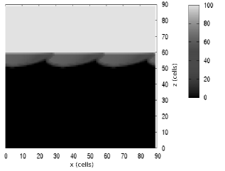
Figure 7: Fluid profile during the penetration into the wood structure. Intensities are identical to Fig. 6. The wood sample is located in the region $y$$<$$60$ with a year ring inclination of $45^{\circ}$.

Discussion and Conclusions

We introduced a new lattice Boltzmann model to simulate the dynamics of the flow of mixtures in anisotropic, heterogeneous porous media. Our 3D model can be applied to many problems in material science and engineering. It includes a free surface technique to simulate the invaded fluid profile inside the material structure and a surface tension term to control the inerface shape dynamics and the forces of cohesion inside the fluid.

The accuracy of the model was tested for a set of simple cases, like generalized Poiseuille flow in isotropic and anisotropic porous media, droplet formation and surface smoothing. We found excellent agreement with the Darcy law for Poiseuille flow. The surface free technique validated in the simulation of a freely falling droplet and its collision against an impermeable and hydrophobic surface showed negligible errors. The surface tension effects were tested by simulating the smoothing of the fluid profile. To demonstrate the applicability of the model to real cases, we implemented a simulation of the penetration of adhesives into a sample of spruce wood. We showed that the model can reproduce the dynamics of hardening fluids in complex materials even when the media are anisotropic and heterogeneous.

The actual model has all the advantages known for the Lattice Boltzmann method like the minimal use computational resources, fast algorithms that allow for real time simulations, and the ability for efficient parallelization. Additionally extensions of the model are rather straightforward. We hope that the proposed simulation approach will be useful in order to model complex geometries in heterogeneous and anisotropic porous media even for complicated fluids like mixtures of two components.

- (1) K. Vafai, Handbook of POROUS MEDIA, second edition edn. (Taylor and Francis Group, LLC, 2005)
- (2) A. Morais, H. Seybold, H. Herrmann, J. J.S. Andrade, Physical Review Letters 103, 194502 (2009)
- (3) C.L. Tien, K. Vafai, Adv. Appl. Mech. 27, 225 (1990)
- (4) C.T. Hsu, P. Cheng, Int. J. Heat Mass Transf. 33, 1587 (1990)
- (5) P. Nithiarasu, K.N. Seetharamu, T. Sundararajan, Int. J. Heat Mass Transf. 40, 3955 (1997)
- (6) J. Bear, Dynamics of Fluids in Porous Media, first edition edn. (Dover Publication, 1972)
- (7) F. Kamke, J. Lee, Wood and Fiber Science 39(2), 205 (2007)
- (8) G.R. McNamara, G. Zanetti, Phys. Rev. Lett. 61, 2332 (1988)
- (9) F. Higuera, S. Succi, R. Benzi, Europhysics Letters 9, 345 (1989)
- (10) E.G. Flekkoy, Phys. Rev. E 54, 5041 (1993)
- (11) B. Chopard, M. Droz, Cellular Automata Modelling of Physical Systems, xii edn. (Cambridge University Press, 1998)
- (12) B. Chopard, P. Luthi, J. Wagen, IEE Proc. Microw. Antennas Propag. 144, 251 (1997)
- (13) S. Succi, R. Benzi, M. Vergassola, Phys. Rev. A 4, 4521 (1991)
- (14) S. Chen, H. Chen, D. Martinez, W. Matthaeus, Phys. Rev. Lett. 67, 3776 (1991)
- (15) M. Mendoza, J.D. Munoz, Physical Review E 77, 026713 (2008)
- (16) S. Succi, R. Benzi, Physica D. 69, 327 (1993)
- (17) T. Reis, T.N. Phillips, J. Phys. A: Math. Theo. 40, 4033 (2007)
- (18) M. Latva-Kokko, D.H. Rothman, Phys. Rev. E 72, 046701 (2005)
- (19) D. Grunau, S. Chen, K. Eggert, Phys. Fluids A 10, 2557 (1993)
- (20) J. Chin, E.S. Boek, P.V. Coveney, Phil. Trans. R. Soc. Lond. A 360, 547 (2002)
- (21) X. Shan, H. Chen, Phys. Rev. E 47, 1815 (1992)
- (22) A.K. Gunstensen, D.H. Rothman, Phys. Rev. A 43, 4320 (1991)
- (23) J. Tolke, M. Krafczyk, M. Schulz, E. Rank, Phil. Trans. R. Soc. Lond. A 360, 535 (2002)
- (24) Z. Guo, T.S. Zhao, Phys. Rev. E 66, 036304 (2002)
- (25) C. Korner, R.F. Singer, Metal Foams and Porous Metal Structures, MIT Publishing pp. 91–96 (1999)
- (26) T. Reis, T.N. Phillips, J. Phys. A: Math. Theor. 40, 4033 (2007)
- (27) P. Bathnagar, E. Gross, , M. Krook, Phys. Rev. 94, 511 (1954)
- (28) Z. Guo, C. Zheng, B. Shi, Physical Review E 65, 046308 (2002)
- (29) S. Succi, The Lattice Boltzmann Equation for Fluid Dynamics and Beyond, first edition edn. (Oxford University Press, 2001)
- (30) U. Frisch, D. d’Humiéres, B. Hasslacher, P. Lallemand, Y. Pomeau, J.P. Rivet, Complex Systems 1, 649 (1987)
- (31) A. Hiorth, U.H. a Lad, S. Evje, S.M. Skjaeveland, Int. J. Numer. Meth. Fluids 59, 405 (2009)
- (32) F. Wittel, G. Dill-Langer, B. Kroeplin, Computational Materials Science 32(3-4), 594 (2004)
- (33) O. Bouriaud, N. Bréda, G.L. Moguédec, G. Nepveu, Trees 18, 264 (2004)
- (34) L. Gibson, M. Ashby, Cellular Solids: Structure and Properties (Cambridge University Press, 1999)
- (35) N. Mouchot, A. Zoulalian, Holzforschung 56, 318 (2002)
- (36) P. Perre, A. Karimi, Maderas, Cienc. tecnol. 4, 50 (2002)
- (37) F.W. H.J. Herrmann, P. Niemz, Tech. rep., Institute for Building Materials (2009), status report to SNF