Companion to
“An update on the Hirsch conjecture”

Abstract

This is an appendix to our paper “An update of the Hirsch Conjecture”, containing proofs of some of the results and comments that were omitted in it.

1 Introduction

This is an appendix to our paper “An update of the Hirsch Conjecture” [39], containing proofs of some of the results and comments that were omitted in it. The numbering of sections and results is the same in both papers, although not all appear in this companion. The same occurs with the bibliography, which we repeat here completely although not all of the papers are referenced. The numbering of figures, however, is correlative. Figures 1 to 6 are in [39] and Figures 7 to 16 are here.

2 Bounds and algorithms

2.1 Small dimension or few facets

*Theorem 2.1 (Klee [40]).

$H(n,3)=\lfloor\frac{2n}{3}\rfloor-1$.

Proof.

To prove the lower bound, we work in the dual setting where our polytope $P$ simplicial and we want to move from one facet to another along the ridges of $P$. Figure 7 shows the graph of a simplicial 3-polytope with nine vertices in which five steps are needed to go from the interior triangle to the most external one (the outer face in the picture, which represents a facet in the polytope). The reader can easily generalize the figure to any number of vertices divisible by three, adding layers of three vertices that increase the diameter by two. For a number of vertices equal to one or two modulo three, simply add one or two vertices in the interior of the central triangle, subdividing it into three or five triangles. One vertex will not increase the diameter, but two vertices will increase it by one.

Figure 7: Construction of simplicial $3$-dimensional polytopes with $3+3k$ vertices and diameter $2k+1$. Two steps are needed to cross each layer of skinny triangles.

For the upper bound, we switch back to simple polytopes. By double-counting, two times the number of edges of a simple $3$-polytope $P$ equals three times its number of vertices. This, together with Euler’s formula, implies that $P$ has exactly $2n-4$ vertices. Let $u$ and $v$ be two of them. Graphs of 3-polytopes are 3-connected (see [3], or [60]), which means that there are three disjoint paths going from $u$ to $v$. Since the number of intermediate vertices available for these three paths to use is $2n-6$, the shortest of them uses at most $\lfloor\frac{2n}{3}\rfloor-2$ vertices, hence it has at most $\lfloor\frac{2n}{3}\rfloor-1$ edges. ∎

It is easy to generalize the second part in the proof to arbitrary dimension, giving the following lower bound. Observe that the formula gives the exact value of $H(n,d)$ for $d=2$ as well.

*Proposition 2.4.

$$H(n,d)\geq\left\lfloor\frac{d-1}{d}n\right\rfloor-(d-2).$$

Proof.

The addition of layers used in the proof of 2.1 can also be described as glueing copies of an octahedron to an already constructed simplicial $3$-polytope. The gluing is along a triangle, so three new vertices are obtained. Before gluing, a projective transformation is made to the octahedron so that the triangle glued is much bigger than the opposite one, which guarantees convexity of the construction.

The generalization to arbitrary dimension is done gluing a cross-polytope, the polar of a $d$-cube. A cross-polytope is also the common convex hull in $\mathbb{R}^{d}$ of two parallel $(d-1)$-simplices opposite to one another. It has $2d$ vertices and to go from a facet to the opposite one $d$ steps are needed. When the cross-polytope is glued to a given polytope its diameter grows by $d-1$, essentially for the same reasons that will make the proof of Theorem 3.16 work. ∎

2.2 General upper bounds on diameters

The proof we offer for Theorem 2.5 is casically taken from Eisenbrand, Hähnle and Rothvoss [25].

*Theorem 2.5 (Larman [45]).

For every $n>d\geq 3$, $H(n,d)\leq n2^{d-3}$.

Proof.

The proof is by induction on $d$. The base case $d=3$ was Theorem 2.1.

Let $u$ be an initial vertex of our polytope $P$, of dimension $d>3$. For each other vertex $v\in\operatorname{vert}(P)$ we consider its distance $d(u_{1},v)$, and use it to construct a sequence of facets $F_{1},\dots,F_{k}$ of $P$ as follows:

• Let $F_{1}$ be a facet that reaches “farthest from $u$” among those containing $u$. That is, let $\delta_{1}$ be the maximum distance to $u$ of a vertex sharing a facet with $u$, and let $F_{1}$ be that facet.

• Let $\delta_{2}$ be the maximum distance to $u$ of a vertex sharing a facet with some vertex at distance $\delta_{1}+1$ from $u$, and let $F_{2}$ be that facet.

• Similarly, while there are vertices at distance $\delta_{i}+1$ from $u$, let $\delta_{i+1}$ be the maximum distance to $u$ of a vertex sharing a facet with some vertex at distance $\delta_{i}+1$ from $u$, and let $F_{i+1}$ be that facet.

We now stratify the vertices of $P$ according to the distances $\delta_{1},\delta_{2},\dots,\delta_{k}$ so obtained. Observe that $\delta_{k}$ is the diameter of $P$. By convention, we let $\delta_{0}=-1$:

$$V_{i}:=\{v\in\operatorname{vert}(P):d(u,v)\in(\delta_{i-1},\delta_{i}]\}.$$

We call a facet $F$ of $P$ active in $V_{i}$ if it contains a vertex of $V_{i}$. The crucial property that our stratification has is that no facet of $P$ is active in more than two $V_{i}$’s. Indeed, each facet is active only in $V_{i}$’s with consecutive values of $i$, but a facet intersecting $V_{i}$, $V_{i+1}$ and $V_{i+2}$ would contradict the choice of the facet $F_{i+1}$. In particular, if $n_{i}$ denotes the number of facets active in $V_{i}$ we have

$$\sum_{i=1}^{k}n_{i}\leq 2n.$$

Since each $F_{i}$ has vertices with distances to $u$ ranging from at least $\delta_{i-1}+1$ to $\delta_{i}$, we have that $\operatorname{diam}(F_{i})\geq\delta_{i}-\delta_{i-1}-1$. Even more, let $Q_{i}$, $i=1,\dots,k$ be the polyhedron obtained by removing from the facet-definition of $F_{i}$ the equations of facets of $P$ that are not active in $V_{i}$ (which may exist since $F_{i}$ may have vertices in $V_{i-1}$). By an argument similar to the one used for the polyhedron $Q$ of the previous proof, $Q_{i}$ has still diameter at least $\delta_{i}-\delta_{i-1}-1$. But, by inductive hypothesis, we also have that the diameter of $Q_{i}$ is at most $2^{d-4}(n_{i}-1)$, since it has dimension $d-1$ and at most $n_{i}-1$ facets. Putting all this together we get the following bound for the diameter $\delta_{k}$ of $P$:

$$\delta_{k} = \sum_{i=1}^{k}(\delta_{i}-\delta_{i-1}-1)+(k-1)$$

$$< \sum_{i=1}^{k}2^{d-4}(n_{i}-1)+k$$

$$= 2^{d-4}\sum_{i}n_{i}-k(2^{d-4}-1)\leq 2^{d-3}n.$$

∎

*Theorem 2.6 (Kalai-Kleitman [36]).

For every $n>d$, $H(n,d)\leq n^{\log_{2}(d)+1}$.

Proof of Theorem 2.6.

Let $P$ be a $d$-dimensional polyhedron with $n$ facets, and let $v$ and $u$ be two vertices of $P$. Let $k_{v}$ (respectively $k_{u}$) be the maximal positive number such that the union of all vertices in all paths in $G(P)$ starting from $v$ (respectively $u$) of length at most $k_{v}$ (respectively $k_{u}$) are incident to at most $\frac{n}{2}$ facets. Clearly, there is a facet $F$ of $P$ so that we can reach $F$ by a path of length $k_{v}+1$ from $v$ and a path of length $k_{u}+1$ from $u$.

We claim that $k_{v}\leq H_{u}(\lfloor\frac{n}{2}\rfloor,d)$ (and the same for $k_{u}$), where $H_{u}(n,d)$ denotes the maximum diameter of all $d$-polyhedra with $n$ facets. To prove this, let $Q$ be the polyhedron defined by taking only the inequalities of $P$ corresponding to facets that can be reached from $v$ by a path of length at most $k_{v}$. By construction, all vertices of $P$ at distance at most $k_{v}$ from $v$ are also vertices in $Q$, and vice-versa. In particular, if $w$ is a vertex of $P$ whose distance from $v$ is $k_{v}$ then its distance from $v$ in $Q$ is also $k_{v}$. Since $Q$ has at most $n/2$ facets, we get $k_{v}\leq H_{u}(\lfloor\frac{n}{2}\rfloor,d)$.

The claim implies the following recursive formula for $H_{u}$:

$$H_{u}(n,d) \leq 2H_{u}\left(\left\lfloor\frac{n}{2}\right\rfloor,d\right)+H_{u}(n,d-1)+2,$$

which we can rewrite as

$$\frac{H_{u}(n,d)+1}{n}\leq\frac{H_{u}\left(\left\lfloor\frac{n}{2}\right\rfloor,d\right)+1}{n/2}+\frac{H_{u}(n,d-1)+1}{n}.$$

This suggests calling $h(k,d):=(H(2^{k},d)-1)/2^{k}$ and applying the recursion with $n=2^{k}$, to get:

$$h(k,d)\leq h(k-1,d)+h(k,d-1).$$

This implies $h(k,d)\leq\binom{k+d}{d}$, or

$$H_{u}(2^{k},d)\leq 2^{k}\binom{k+d}{d}.$$

From this the statement follows if we assume $n\leq 2^{d}$ (that is, $k\leq d$). For $n\geq 2^{d}$ we use Larman’s bound $H_{u}(n,d)\leq n2^{d}\leq n^{2}$, proved below. ∎

2.4 Some polytopes from combinatorial optimization

Small integer coordinates

*Theorem 2.11 (Naddef [50]).

If $P$ is a $0$-$1$ polytope then $\operatorname{diam}(P)\leq n(P)-\dim(P)$.

Proof.

We assume that $P$ is full-dimensional. This is no loss of generality since, if the dimension of $P$ is strictly less than $d$, then $P$ can be isomorphically projected to a face of the cube $[0,1]^{d}$.

Let $u$ and $v$ be two vertices of $P$. By symmetry, we may assume that $u=(0,\ldots,0)$. If there is an $i$ such that $v_{i}=0$, then $u$ and $v$ are both on the face of the cube corresponding to $\{{\bf x}\in\mathbb{R}^{d}\mid x_{i}=0\}$, and the statement follows by induction. Therefore, we assume that $v=(1,\ldots,1)$. Now, pick any neighboring vertex $v^{\prime}$ of $v$. There is an $i$ such that $v^{\prime}_{i}=0$. Then, $u$ and $v^{\prime}$ are vertices of a lower-dimensional $0$-$1$ polytope and we have used one edge to go from $v$ to $v^{\prime}$. The result follows by induction on $d$. ∎

Transportation and dual transportation polytopes

We here include the precise definition of $3$-way transportation polytopes, which we skipped in the paper:

• $3$-way axial transportation polytopes. Let $a=(a_{1},\dots,a_{p})$, $b=(b_{1},\dots,b_{q})$, and $c=(c_{1},\dots,c_{r})$ be three vectors of lengths $p$, $q$ and $r$, respectively. The $3$-way axial $p\times q\times r$ transportation polytope $P$ given by $a\in\mathbb{R}^{p}$, $b\in\mathbb{R}^{q}$, and $c\in\mathbb{R}^{r}$ is defined as follows:

  $$P=\{(x_{ijk})\in\mathbb{R}^{p\times q\times r}\mid\sum_{j,k}x_{ijk}=a_{i},\sum_{i,k}x_{ijk}=b_{j},\sum_{i,j}x_{ijk}=c_{k},x_{ijk}\geq 0\}.$$

  The polytope $P$ has dimension $pqr-(p+q+r-2)$ and at most $pqr$ facets.

• $3$-way planar transportation polytopes. Let $A\in\mathbb{R}^{p\times q}$, $B\in\mathbb{R}^{p\times r}$, and $C\in\mathbb{R}^{q\times r}$ be three matrices. We define the $3$-way planar $p\times q\times r$ transportation polytope $P$ given by $A$, $B$, and $C$ as follows:

  $$P=\{(x_{ijk})\in\mathbb{R}^{p\times q\times r}\mid\sum_{k}x_{ijk}=A_{ij},\sum_{j}x_{ijk}=B_{ik},\sum_{i}x_{ijk}=C_{jk},x_{ijk}\geq 0\}.$$

  It has dimension $(p-1)(q-1)(r-1)$ and at most $pqr$ facets.

2.5 A continuous Hirsch conjecture

Let us expand a bit the concept of curvature of the central path and its relation to the simplex method. For further description of the method we refer to the books [10, 53].

The central path method is one of the interior point methods for solving a linear program. As in the simplex method, the idea is to move from a feasible point to another feasible point on which the given objective linear functional is improved. In contrast to the simplex method, where the path travels from vertex to neighboring vertex along the graph of the feasibility polyhedron $P$, this method follows a certain curve through the strict interior of the polytope.

More precisely, to each linear program,

$$\text{ Minimize }c\cdot{\bf x},\text{ subject to }A{\bf x}={\bf b}\text{ and }{\bf x}\geq 0,$$

the method associates a (primal) central path $\gamma_{c}:[0,\beta)\rightarrow\mathbb{R}^{d}$ which is an analytic curve through the interior of the feasible region and such that $\gamma_{c}(0)$ is an optimal solution of the problem. The central path is well-defined and unique even if the program has more than one optimal solution, but its definition is implicit, so that there is no direct way of computing $\gamma_{c}(0)$. To get to $\gamma_{c}(0)$, one starts at any feasible solution and tries to follow a curve that approaches more and more the central path, using for it certain barrier functions. (Barrier functions play a role similar to the choice of pivot rule in the simplex method. The standard barrier function is the logarithmic function $f(x)=-\sum_{i=1}^{n}\ln(A_{i}x-b_{i})$.)

Of course, it is not possible to follow the curve exactly. Rather, one does Newton-like steps trying not to get too far. How much can one improve in a single step is related to the curvature of the central path: if the path is rather straight one can do long steps without deviating too far from it, if not one needs to use shorter steps. Thus, the total curvature $\lambda_{c}(P)$ of the central path, defined in the usual differential-geometric way, can be considered a continuous analogue of the diameter of the polytope $P$, or at least of the maximum distance from any vertex to a vertex maximizing the functional $c$.

3 Constructions

3.1 The wedge operation

The dual operation to wedging, usually performed for simplicial polytopes (or for simplicial complexes in general), is the one-point suspension. We refer the reader to [19, Section 4.2] for an expanded overview of this topic. Let $w$ be a vertex of the polytope $P$. The one-point suspension of $P\subset\mathbb{R}^{d}$ at the vertex $w$ is the polytope

$$\operatorname{S}_{w}(P):=\operatorname{conv}\big{(}(P\times\{0\})\cup(\{w\}\times\{-1,+1\})\big{)}\subset\mathbb{R}^{d+1}.$$

That is, $\operatorname{S}_{w}(P)$ is formed by taking the convex hull of $P$ (in an ambient space of one higher dimension) with a “raised” and “lowered” copy of the vertex $w$. See Figure 8 for an example.

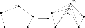
Figure 8: The simplicial version of Figure 3 in [39]: a $5$-gon and a one-point suspension on its topmost vertex

Recasting Lemma 3.1 to the dual setting gives the following simplicial version of it:

Lemma 3.1.

Let $P$ be a $d$-polytope with $n$ vertices. Let $P^{\prime}=\operatorname{S}_{w}(P)$ be its one-point suspension on a certain vertex $w$. Then $P^{\prime}$ is a $(d+1)$-dimensional polytope with $n+1$ vertices, and the diameter of the dual graph of $P^{\prime}$ is at least the diameter of the dual graph of $P$.

The one-point suspension of a simplicial polytope is a simplicial polytope. In fact, the one-point suspension can be described at the leval of abstract simplicial complexes: Let $L$ be a simplicial complex and $w$ a vertex of it. Recall that the anti-star $\operatorname{ast}_{L}(w)$ of $w$ is the subcomplex consisting of simplices not using $w$ and the link $\operatorname{lk}_{L}(w)$ of $w$ is the subcomplex of simplices not using $w$ but joined to $w$. If $L$ is a PL $k$-sphere, then $\operatorname{ast}_{L}(w)$ and $\operatorname{lk}_{L}(w)$ are a $k$-ball and a $(k-1)$-sphere, respectively. The one-point suspension of $L$ at $w$ is the following complex:

$$\operatorname{S}_{w}(L):=(\operatorname{ast}_{L}(w)*w_{1})\cup(\operatorname{ast}_{L}(w)*w_{2})\cup(\operatorname{lk}_{L}(w)*\overline{w_{1}w_{2}}).$$

Here $*$ denotes the join operation: $L*K$ has as simplices all joins of one simplex of $K$ and one of $L$. In Figure 8 the three parts of the formula are the three triangles using $w_{1}$ but not $w_{2}$, the three using $w_{2}$ but not $w_{1}$, and the two using both, respectively.

In Section 3.4 we will make use of an iterated one-point suspension. That is, in $\operatorname{S}_{w}(P)$ we take the one-point suspension over one of the new vertices $w_{1}$ and $w_{2}$, then again in one of the new vertices created, and so on. We leave it to the reader to check that, at the level of simplicial complexes, the one-point suspension iterated $k$ times produces the following simplicial complex, where $\Delta_{k}$ is a $k$-simplex with vertices $w_{1},\dots,w_{k+1}$ and $\partial\Delta_{k}$ is its boundary. Observe that this generalizes the formula for $\operatorname{S}_{w}(L)$ above:

$$\operatorname{S}_{w}(L)^{(k)}:=(\operatorname{ast}_{L}(w)*\partial\Delta_{k})\cup(\operatorname{lk}_{L}(w)*{\Delta_{k}}).$$

3.2 The $d$-step and non-revisiting conjectures

In this section we had proof that for both the Hirsch and the non-revisiting conjectures the general case is equivalent to the case $n=2d$, but we did not finish proving that the two were equivalent:

*Theorem 3.7 (Klee-Walkup [43]).

The Hirsch, non-revisiting, and $d$-step Conjectures 1.1, 3.3, and 3.6 are equivalent.

Proof.

Clearly, the $d$-step conjecture is a special case of both the Hirsch and the non-revisiting conjectures. By Theorems 3.2 and 3.4, to prove that the $d$-step conjecture implies the other two we may restrict our attention to polytopes of dimension $d$ and with $2d$ facets. We also use induction on the codimension. That is, we assume the Hirsch and non-revisiting conjectures for all polytopes with number of facets minus dimension smaller than $d$.

Let $u$ and $v$ be two vertices of a $d$-polytope $P$ with $2d$ facets. We will also induct on the number of common facets containing both $u$ and $v$. The base case is when $u$ and $v$ are complementary, in which the $d$-step conjecture applied to them gives a non-revisiting path of length at most $d$.

So, we assume that $u$ and $v$ are in a common facet $F$ of $P$. $F$ has at most $2d-1$ facets itself.

• If $F$ has less than $2d-1$ facets, then $F$ has the non-revisiting and Hirsch properties by induction on “number of facets minus dimension”, and we are done.

• If $F$ has $2d-1$ facets, since it has dimension $d-1$ there is a facet $G$ of $F$ not containing $u$ nor $v$. Let $P^{\prime}=\operatorname{W}_{G}(F)$ be the wedge of $F$ on $G$. Let $u_{1}$ and $v_{2}$ be vertices of $P^{\prime}$ projecting to vertices $u$ and $v$ of $P$ and such that $F_{1}$ contains $u_{1}$ and $F_{2}$ contains $v_{2}$. As in the proof of Theorem 3.4, $F_{1}$ and $F_{2}$ denote the non-vertical facets of the wedge $P^{\prime}$. $P^{\prime}$ again has dimension $d$ and $2d$ facets, but its vertices $u_{1}$ and $v_{2}$ have one less facet in common than $u$ and $v$ had. By induction on the number of common facets, there is a non-revisiting path of length at most $d$ between $u_{1}$ and $v_{2}$ in $P^{\prime}$. When this path is projected to $F$, it retains the non-revisiting property and its length does not increase.

∎

3.3 The Klee-Walkup polytope $Q_{4}$

Let us give further details on the structure of the Hisrsch-sharp polytope $Q_{4}$ constructed by Klee and Walkup. Recall that the coordinates we use for the nine vertices of $Q_{4}$ are:

$$w:=(0,0,0,-2)$$,

, ,

, ,

, .

What follows is the input and output of the polymake [28] computation of the face complex of $Q_{4}$. The input vertices are given in homogenized version, which means and additional coordinate of 1’s is added to each.

POINTS
 1  0  0  0 -2
 1 -3  3  1  2
 1  3 -3  1  2
 1  2 -1  1  3
 1 -2  1  1  3
 1  3  3 -1  2
 1 -3 -3 -1  2
 1 -1 -2 -1  3
 1  1  2 -1  3

The output VERTICES_IN_FACETS lists the facets as sets of vertices. Polymake numbers the vertices starting with 0, so our vertices $w,a,\dots,h$ become labeled 0, 1,…,8:

VERTICES_IN_FACETS
 {2 3 7 8}
 {0 1 2 3}
 {1 2 3 4}
 {2 3 6 7}
 {2 3 4 6}
 {0 2 4 6}
 {0 2 6 7}
 {0 1 2 4}
 {1 6 7 8}
 {0 1 6 8}
 {1 4 7 8}
 {0 1 4 6}
 {1 4 6 7}
 {3 4 6 7}
 {3 4 7 8}
 {0 5 6 8}
 {5 6 7 8}
 {0 1 5 8}
 {1 4 5 8}
 {3 4 5 8}
 {0 1 3 5}
 {1 3 4 5}
 {0 5 6 7}
 {0 2 5 7}
 {2 5 7 8}
 {0 2 3 5}
 {2 3 5 8}

You should verify that there are exactly 15 tetrahedra not using $w$ (the label 0) are precisely the ones in Figure 9.

$$\begin{matrix}&&\textbf{{abcd}}&&&&&&&\\ &&|&&&&&&&\\ &&acde&&&&&&&\\ &&|&\diagdown&&&&&&\\ &&adeh&\text{---}&cdeh&\text{---}&bceh&\text{---}&begh&\text{---}\quad\textbf{{efgh}}\\ &&|&&|&&|&\diagup&&\\ &&adgh&\text{---}&cdgh&\text{---}&bcgh&&&\\ &\diagup&|&&|&&|&&&\\ \textbf{{efgh}}\quad\text{---}\quad afgh&\text{---}&adfg&\text{---}&cdfg&\text{---}&bcfg&&&\\ &&&&&\diagdown&|&&&\\ &&&&&&bcdf&&&\\ &&&&&&|&&&\\ &&&&&&\textbf{{abcd}}&&&\\ \end{matrix}$$

Figure 9: The dual graph of the subcomplex $K$

From the picture we can also read the tetrahedra of $\partial Q_{4}^{*}$ that use $w$: there is one for each triangle that appears only once in the list. For example, since $abcd$ is adjacent only to $acde$ and $abcd$, the triangles $abc$ and $bcd$ are joined to $w$ . The boundary of the antistar of $w$, that is, the link of $w$ in $Q_{4}^{*}$ turns out to be, combinatorially, the triangulation of the boundary of a cube displayed in Figure 10.

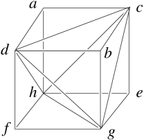
Figure 10: The link of $w$ in $Q_{4}$ is combinatorially a triangulation of the boundary of a cube.

The anti-star $K$ of $w$ in $\partial Q_{4}^{*}$ is a topological triangulation of the interior of the cube. But we need to deform the cube a bit to realize this triangulation geometrically. This is shown in Figure 11: the quadrilaterals $abcd$ and $efgh$ are displayed separately as lying in two different horizontal planes (so that the two relevant tetrahedra $abcd$ and $efgh$ degenerate to flat quadrilaterals), and the central part of the figure shows the intersection of $K$ with their bisecting plane. Tetrahedra with three points on one plane and one in the other appear as triangles and tetrahedra with two points on either side appear as quadrilaterals. The tetrahedra $abcd$ and $efgh$ do not show up in the figure, since they do not intersect the intermediate plane. For the interested reader, this picture is an example of a mixed subdivision of the Minkowski sum of two polygons. The fact that triangulations of polytopes with their vertices lying in two parallel hyperplanes can be pictured as mixed subdivisions is the polyhedral Cayley trick [19, Chapter 9].

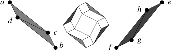
Figure 11: The Klee-Walkup complex as a mixed subdivision. The shadowed triangles represent tetrahedra adjacent to $abcd$ and $efgh$

3.4 Many Hirsch-sharp polytopes?

Trivial Hirsch-sharp polytopes

*Proposition 3.10.

For every $n\geq d$ there are simple unbounded $d$-polyhedra with $n$ facets and diameter $n-d$.

Proof.

The proof is by induction on $n$, the base case $n=d$ being the orthant $\{x_{i}\geq 0,\forall i\}$. Our inductive hypothesis is not only that we have constructed a $d$-polyhedron $P$ with $n-1$ facets and diameter $n-d-1$; also, that vertices $u$ and $v$ at distance $n-d-1$ exist in it with $v$ incident to some unbounded ray $l$. Let $H$ be a supporting hyperplane of $l$, and tilt it slightly at a point $v^{\prime}$ in the interior of $l$ to obtain a new hyperplane $H^{\prime}$. See Figure 12. Then, the polyhedron $P^{\prime}$ obtained cutting $P$ with the tilted hyperplane $H^{\prime}$ has $n$ facets and diameter $n-d$; $v$ is the only vertex adjacent to $v^{\prime}$ in the graph, so we need at least $1+(n-d-1)$ steps to go from $v^{\prime}$ to $u$. ∎

Figure 12: Tilting the hyperplane $H$, example in dimension two

Non-trivial Hirsch-sharp polytopes

In [39] we only proved part (1) of the following result:

*Theorem 3.11 (Fritzsche-Holt-Klee [27, 31, 32]).

Hirsch-sharp $d$-polytopes with $n$ facets exist in at least the following cases: (1) $n\leq 3d-3$; and (2) $d\geq 7$.

The proof of part (2) is easier to understand in the simplicial framework. So, as a warm-up, we include (see Figure 13) the simplicial version of [39, Figure 5]. We already know that the polar of wedging is one-point suspension. The polar of truncation of a vertex is the stellar subdivision of a facet by adding to our polytope a new vertex very close to that facet.

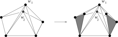
Figure 13: The simplicial version of [39, Figure 5]. Wedging becomes one-point suspension and truncation is stellar subdivision

The key property in the proof of Lemma 3.12 is that the wedge and one-point suspension operations do not only preserve Hirsch-sharpness; they also increase the number of vertices or facets (respectively) that are at Hirsch distance from one another. This suggests looking at what happens when we iterate the process. The answer, that we state in the simplicial version, is as follows:

Lemma 3.14 (Holt-Klee [32]).

Let $P$ be a simplicial $d$-polytope with more than $2d$ vertices. Let $A$ and $B$ be two facets of it at Hirsch distance in the dual graph and let $w$ be a vertex contained in neither $A$ nor $B$. Let $P^{(k)}$ be the $k^{\textrm{th}}$ one-point suspension of $P$ on the vertex $w$.

Then, $P^{(k)}$ has two $(k+1)$-tuples of facets $\{A_{1},\dots,A_{k+1}\}$ and $\{B_{1},\dots,B_{k+1}\}$ with every $A_{i}$ at Hirsch distance from every $B_{i}$. All the facets in each tuple are adjacent to one another.

Proof.

We use the following formula, from Section 3.1, for the iterated one-point suspension of the simplicial complex $L=\partial P$:

$$\operatorname{S}_{w}(L)^{(k)}:=(\operatorname{ast}_{L}(w)*\partial\Delta_{k})\cup(\operatorname{lk}_{L}(w)*{\Delta_{k}}).$$

Here $\Delta_{k}$ is a $k$-simplex. The two groups of facets in the statement are $A*\partial\Delta_{k}$ and $B*\partial\Delta_{k}$. The details are left to the interested reader. ∎

Proof of part (2) of Theorem 3.11..

We include only the proof for the case $d\geq 8$, contained in [27]. The improvement to $d=7$ was later found by Holt [31].

Both are based on a new operation on polytopes that we now introduce. The version for simple polytopes is called blending, but we describe it for simplicial polytopes and call it glueing. Glueing is simply a combinatorial/geometric version of the connected sum of topological manifolds. Let $P_{1}$ and $P_{2}$ be two simplicial $d$-polytopes and let $F_{1}$ and $F_{2}$ be respective facets. The manifolds are $\partial P_{1}$ and $\partial P_{2}$ (two $(d-1)$-spheres); from them we remove the interiors of $F_{1}$ and $F_{2}$ after which we glue their boundaries. See Figure 14, where the operation is performed on two facets of the same polytope. On the top part we glue the polytopes “as they come”, which does not preserve convexity. But if projective transformations are made on $P_{1}$ and $P_{2}$ that send points that are close to $F_{1}$ and $F_{2}$ to infinity, then the glueing preserves convexity, so it yields a polytope that we denote $P_{1}\#P_{2}$. This is shown on the bottom part of the Figure.

Figure 14: Glueing two simplicial polytopes along one facet. In the version on the bottom, a projective transformation is done to $P_{1}$ and $P_{2}$ before glueing, to guarantee convexity of the outcome

Glueing almost adds the diameters of the two original polytopes. Suppose that the facets $F_{1}$ and $F_{2}$ are at distances $\delta_{1}$ and $\delta_{2}$ to certain facets $F^{\prime}_{1}$ and $F^{\prime}_{2}$ of $P_{1}$ and $P_{2}$. Then, to go from $F^{\prime}_{1}$ to $F^{\prime}_{2}$ in $P_{1}\#P_{2}$ we need at least $(\delta_{1}-1)+1+(\delta_{2}-1)=\delta_{1}+\delta_{2}-1$ steps.

But we can do better if we combine glueing with the iterated one-point suspension. Consider the simplicial Klee-Walkup $4$-polytope $Q_{4}^{*}$ described in Section 3.3 and let $A$ and $B$ two facets of it at distance five. Let $P^{\prime}$ be the $4^{\textrm{th}}$ one-point suspension of it on the vertex $w$ not contained in $A\cup B$. Observe that $P^{\prime}$ has 13 vertices and dimension eight. By the lemma, $P^{\prime}$ has two groups of five facets $\{A_{1},\dots,A_{5}\}$ and $\{B_{1},\dots,B_{5}\}$ with every $A_{i}$ at Hirsch distance from every $B_{i}$ and all the facets in each group adjacent to one another.

We now glue several copies of $P^{\prime}$ to one another, a $B_{i}$ from each copy glued to an $A_{i}$ of the next one. Each glueing adds five vertices and, in principle, four to the diameter. But Lemma 3.14 implies the following nice property for $P^{\prime}$: half of the eight facets adjacent to each $A_{i}$ are at distance four to half of the facets adjacent to each $B_{i}$. Using the language of Fritzsche, Holt and Klee, we call those facets the slow neighbors of each $A_{i}$ or $B_{i}$, and call the others fast. Since half of the total neighbors are slow, we can make all glueings so that every fast neighbor is glued to a slow one and vice-versa. This increases the diameter by one at every glueing, and the result is Hirsch-sharp.

The above construction yields Hirsch-sharp 8-polytopes with $13+5k$ vertices, for every $k\geq 0$. We can get the intermediate values of $n$ too, via truncation. By Lemma 3.12, every time we do a one-point suspension on a Hirsch-sharp simplicial polytope we can increase the number of facets by one or two via a stellar subdivision at each end. Since the polytope $P^{\prime}$ we are glueing is a 4-fold one-point suspension, and since there are two ends that remain unglued (the $A$-face of the first copy and the $B$-face of the last) we can do up to eight stellar subdivisions to it and still preserve Hirsch-sharpness. ∎

3.5 The unbounded and monotone Hirsch conjectures are false

*Theorem 3.16 (Todd [57]).

There is a simple bounded polytope $P$, two vertices $u$ and $v$ of it, and a linear functional $\phi$ such that:

1. $v$ is the only maximal vertex for $\phi$.

2. Any edge-path from $u$ to $v$ and monotone with respect to $\phi$ has length at least five.

Proof.

Let $Q_{4}$ be the Klee-Walkup polytope. Let $F$ be the same “ninth facet” as in the previous proof, one that is not incident to the two vertices $u$ and $v$ that are at distance five from each other. Let $H_{2}$ be the supporting hyperplane containing $F$ and let $H_{1}$ be any supporting hyperplane at the vertex $v$. Finally, let $H_{0}$ be a hyperplane containing the (codimension two) intersection of $H_{1}$ and $H_{2}$ and which lies “slightly beyond $H_{1}$”, as in Figure 15. (Of course, if $H_{1}$ and $H_{2}$ happen to be parallel, then $H_{0}$ is taken to be parallel to them and close to $H_{1}$.) The exact condition we need on $H_{0}$ is that it does not intersect $Q_{4}$ and the small, wedge-shaped region between $H_{0}$ and $H_{1}$ does not contain the intersection of any 4-tuple of facet-defining hyperplanes of $Q_{4}$.

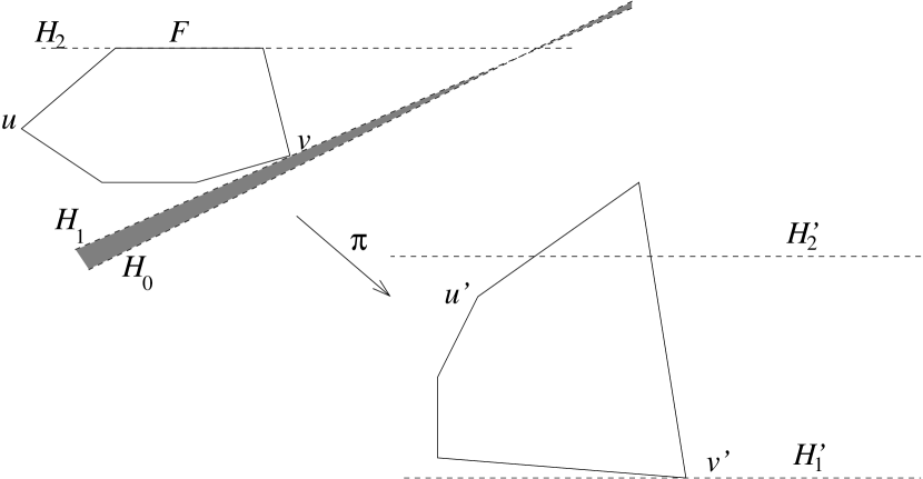
Figure 15: Disproving the monotone Hirsch conjecture

We now make a projective transformation $\pi$ that sends $H_{0}$ to be the hyperplane at infinity. In the polytope $Q^{\prime}_{4}=\pi(Q_{4})$ we “remove” the facet $F^{\prime}=\pi(F)$ that is not incident to the two vertices $u^{\prime}=\pi(u)$ and $v^{\prime}=\pi(v)$. That is, we consider the polytope $Q^{\prime\prime}_{4}$ obtained from $Q^{\prime}_{4}$ by forgetting the inequality that creates the facet $F^{\prime}$ (see Figure 15 again). Then $Q^{\prime\prime}_{4}$ will have new vertices not present in $Q^{\prime}_{4}$, but it also has the following properties:

1. $Q^{\prime\prime}_{4}$ is bounded. Here we are using the fact that the wedge between $H_{0}$ and $H_{1}$ contains no intersection of facet-defining hyperplanes: this implies that no facet of $Q^{\prime\prime}_{4}$ can go “past infinity”.

2. It has eight facets: four incident to $u^{\prime}$ and four incident to $v^{\prime}$.

3. The functional $\phi$ that is maximized at $v^{\prime}$ and constant on its supporting hyperplane $H^{\prime}_{1}=\pi(H_{1})$ is also constant on $H^{\prime}_{2}=\pi(H_{2})$, and $u^{\prime}$ lies on the same side of $H^{\prime}_{1}$ as $v^{\prime}$.

In particular, no $\phi$-monotone path from $u^{\prime}$ to $v^{\prime}$ crosses $H^{\prime}_{1}$, which means it is also a path from $u^{\prime}$ to $v^{\prime}$ in the polytope $Q^{\prime}_{4}$, combinatorially isomorphic to $Q_{4}$. ∎

3.6 The topological Hirsch conjecture is false

*Theorem 3.18 (Mani-Walkup [46]).

There is a triangulated 3-sphere with 16 vertices and without the non-revisiting property. Wedging on it eight times yields a non-Hirsch $11$-sphere with $24$ vertices.

Proof.

The key part of the construction is the two-dimensional simplicial complex $K$ consisting of the following 32 triangles:

amr mbr bnr ncr cor odr dpr par

amt mbt bnt nct cot odt dpt pat

aoq obq bpq pcq cmq mdq dnq naq

 aos obs bps pcs cms mds dns nas

The first and second halves are topological 2-spheres, triangulated in the form of double pyramids over the octagons $ambncodp$ and $aobpcmdn$ (same vertices, but in different order). Observe that in both octagons every edge goes from one of $\{a,b,c,d\}$ to one of $\{m,n,o,p\}$, but the vertices are shuffled in such a way that no edge is repeated. See Figure 16.

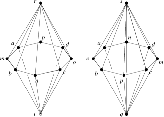
Figure 16: Two octagonal bipyramids

The interiors of the two bipyramids can easily be triangulated (subdivided into terahedra) in such a way that the tetrahedron $abcd$ is used in the first one and $mnop$ in the second. Then the two bipyramids can be embedded in the $3$-sphere (with corresponding vertices identified) by first embedding them disjointly and then pinching the vertices of one of the octagons to glue them with those of the other. We claim that no extension of this partial triangulation to the whole $3$-sphere can have the non-revisiting property.

Indeed, every path from the tetrahedron $abcd$ to the tetrahedron $mnop$ must exit the first bipyramid through one of its boundary triangles, which uses one of the edges of the first octagon. In particular, our path will at this point have abandoned three of the vertices of $abcd$ and be using one of $mnop$. To keep the non-revisiting property, the abandoned vertices should not be used again, and the new one should not be abandoned, since it is a vertex of our target tetrahedron. But then it is impossible for our path to enter the second bipyramid: it should do so via a triangle using an edge of the second octagon, and non-revisiting implies that this edge should be the same used to exit the first bipyramid. This is impossible since the two octagons have no edge in common.

We skip the technical part of the proof, namely that $K$ can be completed to a triangulation of the $3$-sphere using the tetrahedra $abcd$ and $mnop$ (and with only four extra vertices). The way Mani and Walkup show it is by listing the tetrahedra of the whole triangulation and verifying that they form a shellable sphere. ∎

Edward D. Kim
Department of Mathematics
University of California, Davis. Davis, CA 95616, USA
email: ekim@math.ucdavis.edu
web: http://www.math.ucdavis.edu/~ekim/

Francisco Santos
Departamento de Matemáticas, Estadística y Computación
Universidad de Cantabria, E-39005 Santander, Spain
email: francisco.santos@unican.es
web: http://personales.unican.es/santosf/

References

- [1] A. Altshuler. The Mani-Walkup spherical counterexamples to the -path conjecture are not polytopal. Math. Oper. Res., 10(1):158–159, 1985.
- [2] A. Altshuler, J. Bokowski, and L. Steinberg. The classification of simplicial -spheres with nine vertices into polytopes and non-polytopes. Discrete Math., 31:115–124, 1980.
- [3] M. L. Balinski. On the graph structure of convex polyhedra in -space. Pacific J. Math., 11:431–434, 1961.
- [4] M. L. Balinski. The Hirsch conjecture for dual transportation polyhedra. Math. Oper. Res., 9(4):629–633, 1984.
- [5] D. Barnette. paths on 3-polytopes. J. Combinatorial Theory, 7:62–70, 1969.
- [6] M. Beck, S. Robins, Computing the continuous discretely. Integer-point enumeration in polyhedra. Undergraduate Texts in Mathematics. Springer, 2007.
- [7] A. Björner, F. Brenti, Combinatorics of Coxeter Groups, Graduate Texts in Mathematics, 231, Springer-Verlag, 2005.
- [8] L. Blum, F. Cucker, M. Shub, and S. Smale, Complexity and real computation, Springer-Verlag, 1997.
- [9] K. H. Borgwardt, The Average Number of Steps Required by the Simplex Method Is Polynomial. Zeitschrift fur Operations Research, 26:157–77, 1982.
- [10] S. Boyd and L. Vandenberghe. Convex Optimization. Cambridge University Press, Cambridge, 2004.
- [11] D. Bremner, A. Deza, W. Hua, and L. Schewe. More bounds on the diameter of convex polytopes: . (in preparation)
- [12] D. Bremner and L. Schewe. Edge-graph diameter bounds for convex polytopes with few facets.
- [13] G. Brightwell, J. van den Heuvel, and L. Stougie. A linear bound on the diameter of the transportation polytope. Combinatorica, 26(2):133–139, 2006.
- [14] W. H. Cunningham. Theoretical properties of the network simplex method. Math. Oper. Res., 4:196–208, 1979.
- [15] G. B. Dantzig, Linear programming and extensions, Princeton University Press, 1963.
- [16] J. A. De Loera, E. D. Kim, S. Onn, and F. Santos. Graphs of transportation polytopes. J. Combin. Theory Ser. A, 116(8):1306–1325, 2009.
- [17] J. A. De Loera. The many aspects of counting lattice points in polytopes. Math. Semesterber. 52(2):175–195, 2005.
- [18] J. A. De Loera and S. Onn. All rational polytopes are transportation polytopes and all polytopal integer sets are contingency tables. In Lec. Not. Comp. Sci., volume 3064, pages 338–351, New York, NY, 2004. Proc. 10th Ann. Math. Prog. Soc. Symp. Integ. Prog. Combin. Optim. (Columbia University, New York, NY, June 2004), Springer-Verlag.
- [19] J. A. De Loera, J. Rambau, F. Santos, Triangulations: Applications, Structures and Algorithms. Algorithms and Computation in Mathematics (to appear).
- [20] J.-P. Dedieu, G. Malajovich, and M. Shub. On the curvature of the central path of linear programming theory. Found. Comput. Math. 5:145–171, 2005.
- [21] A. Deza, T. Terlaky, and Y. Zinchenko. Central path curvature and iteration-complexity for redundant Klee-Minty cubes. Adv. Mechanics and Math., 17:223–256, 2009.
- [22] A. Deza, T. Terlaky, and Y. Zinchenko. A continuous -step conjecture for polytopes. Discrete Comput. Geom., 41:318–327, 2009.
- [23] A. Deza, T. Terlaky, and Y. Zinchenko. Polytopes and arrangements: Diameter and curvature. Oper. Res. Lett., 36(2):215–222, 2008.
- [24] M. Dyer and A. Frieze. Random walks, totally unimodular matrices, and a randomised dual simplex algorithm. Math. Program., 64:1–16, 1994.
- [25] F. Eisenbrand, N. Hähnle, A. Razborov, and T. Rothvoß. Diameter of Polyhedra: Limits of Abstraction. 2009. (in preparation)
- [26] S. Fomin and A. Zelevinsky. -systems and generalized associahedra. Ann. of Math. 158(2), 977–1018, 2003.
- [27] K. Fritzsche and F. B. Holt. More polytopes meeting the conjectured Hirsch bound. Discrete Math., 205:77–84, 1999.
- [28] E. Gawrilow, M. Joswig. Polymake: A software package for analyzing convex polytopes. Software available at http://www.math.tu-berlin.de/polymake/
- [29] D. Goldfarb and J. Hao. Polynomial simplex algorithms for the minimum cost network flow problem. Algorithmica, 8:145–160, 1992.
- [30] P. R. Goodey. Some upper bounds for the diameters of convex polytopes. Israel J. Math., 11:380–385, 1972.
- [31] F. B. Holt. Blending simple polytopes at faces. Discrete Math., 285:141–150, 2004.
- [32] F. Holt and V. Klee. Many polytopes meeting the conjectured Hirsch bound. Discrete Comput. Geom., 20:1–17, 1998.
- [33] C. Hurkens. Personal communication, 2007.
- [34] G. Kalai. A subexponential randomized simplex algorithm. In Proceedings of the 24th annual ACM symposium on the Theory of Computing, pages 475–482, Victoria, 1992. ACM Press.
- [35] G. Kalai. Online blog http://gilkalai.wordpress.com. See for example http://gilkalai.wordpress.com/2008/12/01/a-diameter-problem-7/, December 2008.
- [36] G. Kalai and D. J. Kleitman. A quasi-polynomial bound for the diameter of graphs of polyhedra. Bull. Amer. Math. Soc., 26:315–316, 1992.
- [37] N. Karmarkar. A new polynomial time algorithm for linear programming. Combinatorica, 4(4):373–395, 1984.
- [38] L. G. Hačijan. A polynomial algorithm in linear programming. (in Russian) Dokl. Akad. Nauk SSSR, 244(5):1093–1096, 1979.
- [39] E. D. Kim, and F. Santos. An update on the Hirsch conjecture, preprint 2009, version 2. http://arxiv.org/abs/0907.1186v2.
- [40] V. Klee. Paths on polyhedra II. Pacific J. Math., 17(2):249–262, 1966.
- [41] V. Klee, P. Kleinschmidt, The -Step Conjecture and Its Relatives, Mathematics of Operations Research, 12(4):718–755, 1987.
- [42] V. Klee, G. J. Minty, How good is the simplex algorithm?, in Inequalities, III (Proc. Third Sympos., Univ. California, Los Angeles, Calif., 1969; dedicated to the memory of Theodore S. Motzkin), Academic Press, New York, 1972, pp. 159–175.
- [43] V. Klee and D. W. Walkup. The -step conjecture for polyhedra of dimension . Acta Math., 133:53–78, 1967.
- [44] P. Kleinschmidt and S. Onn. On the diameter of convex polytopes. Discrete Math., 102(1):75–77, 1992.
- [45] D. G. Larman. Paths of polytopes. Proc. London Math. Soc., 20(3):161–178, 1970.
- [46] P. Mani and D. W. Walkup. A -sphere counterexample to the -path conjecture. Math. Oper. Res., 5(4):595–598, 1980.
- [47] J. Matoušek, M. Sharir, and E. Welzl. A subexponential bound for linear programming. In Proceedings of the 8th annual symposium on Computational Geometry, pages 1–8, 1992.
- [48] N. Megiddo. Linear programming in linear time when the dimension is fixed. J. Assoc. Comput. Mach., 31(1):114–127, 1984.
- [49] N. Megiddo. On the complexity of linear programming. In: Advances in economic theory: Fifth world congress, T. Bewley, ed. Cambridge University Press, Cambridge, 1987, 225-268.
- [50] D. Naddef. The Hirsch conjecture is true for -polytopes. Math. Program., 45:109–110, 1989.
- [51] T. Oda, Convex bodies and algebraic geometry, Springer Verlag, 1988.
- [52] J. B. Orlin. A polynomial time primal network simplex algorithm for minimum cost flows. Math. Program., 78:109–129, 1997.
- [53] J. Renegar. A Mathematical View of Interior-Point Methods in Convex Optimization. SIAM, 2001.
- [54] S. Smale, On the Average Number of Steps of the Simplex Method of Linear Programming. Mathematical Programming, 27: 241-62, 1983.
- [55] S. Smale, Mathematical problems for the next century. Mathematics: frontiers and perspectives, pp. 271–294, American Mathematics Society, Providence, RI (2000).
- [56] D. A. Spielman and S. Teng. Smoothed analysis of algorithms: Why the simplex algorithm usually takes polynomial time. J. ACM, 51(3):385–463, 2004.
- [57] M. J. Todd. The monotonic bounded Hirsch conjecture is false for dimension at least , Math. Oper. Res., 5:4, 599–601, 1980.
- [58] R. Vershynin. Beyond Hirsch conjecture: walks on random polytopes and smoothed complexity of the simplex method. In IEEE Symposium on Foundations of Computer Science, volume 47, pages 133–142. IEEE, 2006.
- [59] D. W. Walkup. The Hirsch conjecture fails for triangulated -spheres. Math. Oper. Res., 3:224-230, 1978.
- [60] G. M. Ziegler, Lectures on polytopes, Graduate Texts in Mathematics, 152, Springer-Verlag, 1995.
- [61] G. M. Ziegler, Face numbers of 4-polytopes and 3-spheres. Proceedings of the International Congress of Mathematicians, Vol. III (Beijing, 2002), Higher Ed. Press, Beijing, 2002, pp. 625–634.