Phase gate of one qubit simultaneously controlling $n$ qubits in a cavity

Abstract

We propose how to realize a three-step controlled-phase gate of one qubit simultaneously controlling $n$ qubits in a cavity or coupled to a resonator. The $n$ two-qubit controlled-phase gates, forming this multiqubit phase gate, can be performed simultaneously. The operation time of this phase gate is independent of the number $n$ of qubits. This phase gate controlling at once $n$ qubits is insensitive to the initial state of the cavity mode and can be used to produce an analogous CNOT gate simultaneously acting on $n$ qubits. We present two alternative approaches to implement this gate. One approach is based on tuning the qubit frequency while the other method tunes the resonator frequency. Using superconducting qubits coupled to a resonator as an example, we show how to implement the proposed gate with one superconducting qubit simultaneously controlling $n$ qubits selected from $N$ qubits coupled to a resonator ($1<n<N$). We also give a discussion on realizing the proposed gate with atoms, by using one cavity initially in an arbitrary state.

I. INTRODUCTION

Quantum information processing has attracted considerable interest during the past decade. The building blocks of quantum computing are single-qubit and two-qubit logic gates. So far, a large number of theoretical proposals for realizing two-qubit gates in many physical systems, such as trapped ions, atoms in cavity QED, nuclear magnetic resonance (NMR), and solid-state devices, have been proposed. Moreover, two-qubit controlled-not (CNOT), controlled-phase (CP), $i$SWAP gates, or other two-qubit operations have been experimentally demonstrated in ion traps [1], NMR [2], quantum dots [3], and superconducting qubits [4-8].

In recent years, analogs of cavity quantum electrodynamics (QED) have been studied using superconducting Josephson devices. There, a superconducting resonator provides a quantized cavity field, superconducting qubits act as artificial atoms, and the strong coupling between the field and superconducting qubits has been demonstrated [9]. Theoretically, many approaches for performing two-qubit logic gates using superconducting qubits coupled to a superconducting resonator or cavity have been proposed [e.g., 10-15]. Moveover, experimental demonstrations of two-qubit gates or two-qubit operations using superconducting qubits coupled to cavities have recently been reported [7,8].

Attention is now shifting to the physical realization of multi-qubit gates (see, e.g., Ref. [16]) instead of just two-qubit gates. It is known that any multi-qubit gate can be decomposed into two-qubit gates and one-qubit gates. When using the conventional gate-decomposition protocols to construct a multi-qubit gate [17,18], the procedure usually becomes complicated as the number of qubits increases. Therefore, building a multi-qubit gate may become very difficult since each elementary gate requires turning on and off a given Hamiltonian for a certain period of time, and each additional basic gate adds experimental complications and the possibility of more errors. During the past few years, several methods for constructing multi-qubit phase gates with $n$-control qubits acting on one target qubit based on ion traps [19], cavity QED [20,21], or circuit QED [22] have been proposed. As is well known, a multi-qubit gate with multiple control qubits controlling a single qubit plays a significant role in quantum information processing, such as quantum algorithms [e.g.,23,24] and quantum error-correction protocols [25].

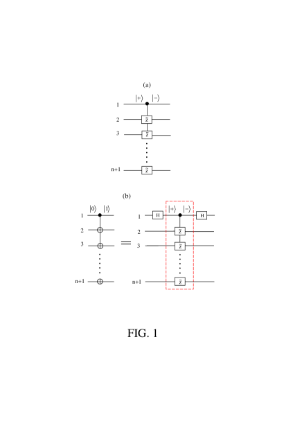
Figure 1: (Color online) (a) Schematic circuit of a $n$-target-qubit control phase (NTCP) gate with qubit 1 simultaneously controlling $n$ target qubits (2, 3, …, $n+1$). The NTCP gate is equivalent to $n$ two-qubit control phase (CP) gates each having a shared control qubit (qubit 1) but a different target qubit (either qubit 2, 3, …, or $n+1$).  Here, $\widetilde{Z}$ represents a controlled-phase flip on each target qubit, with respect to the computational basis formed by the two eigenstates $\left|+\right\rangle$ and $\left|-\right\rangle$ of the Pauli operator $\sigma_{x}.$ Namely, if the control qubit 1 is in the state $\left|-\right\rangle$, then the state $\left|-\right\rangle$ at each $\widetilde{Z}$ is phase-flipped as $\left|-\right\rangle$ $\rightarrow-\left|-\right\rangle$, while the state $\left|+\right\rangle$ remains unchanged. (b) Relationship between a $n$-target-qubit controlled-NOT gate and a NTCP gate. The circuit on the left side of (b) is equivalent to the circuit on the right side of (b). For the circuit on the left side, the symbol $\oplus$ represents a NOT gate on each target qubit, with respect to the computational basis formed by the two eigenstates $\left|0\right\rangle$ and $\left|1\right\rangle$ of the Pauli operator $\sigma_{z}$. If the control qubit 1 is in the state $\left|1\right\rangle$, then the state at $\oplus$ is bit flipped as $\left|1\right\rangle$ $\rightarrow\left|0\right\rangle$ and $\left|0\right\rangle$ $\rightarrow\left|1\right\rangle$. However, when the control qubit 1 is in the state $\left|0\right\rangle$, the state at $\oplus$ remains unchanged. On the other hand, for the circuit on the right side, the part enclosed in the (red) dashed-line box represents a NTCP gate. The element containing H corresponds to a Hadamard transformation described by $\left|0\right\rangle\rightarrow\left|+\right\rangle=\left(1/\sqrt{2}\right)\left(\left|0\right\rangle+\left|1\right\rangle\right)$, and $\left|1\right\rangle\rightarrow\left|-\right\rangle=\left(1/\sqrt{2}\right)\left(\left|0\right\rangle-\left|1\right\rangle\right).$

In this work, we focus on another type of multi-qubit gates, i.e., a multi-qubit phase gate with one control qubit simultaneously controlling $n$ target qubits. This multi-qubit gate is useful in quantum information processing such as entanglement preparation [26], error correction [27], quantum algorithms (e.g., the Discrete Cosine Transform [28]), and quantum cloning [29]. In the following, we will propose a way for realizing this multi-qubit gate using ($n+1$) qubits in a cavity or coupled to a resonator. To implement this gate, we construct an effective Hamiltonian which contains interaction terms between the control qubit and each subordinate or target qubit. We will denote this $n$-target-qubit control-phase gate as an NTCP gate [Fig. 1(a)]. We present two alternative approaches to implement this NTCP gate. One approach is based on tuning the qubit frequency, while the other method tunes the cavity (or resonator) frequency. We present these two alternative methods because some experimental implementations might find it easier to tune the qubit frequency, while others might prefer to tune the cavity frequency. For solid state qubits such as superconducting qubits and semiconductor quantum dots, the qubit transition frequency (or the qubit level spacings) can be readily adjusted by varying the external parameters [30-34] (e.g., the external magnetic flux for superconducting charge qubits, the flux bias or current bias in the case of superconducting phase qubits and flux qubits, see e.g. [30-33], and the external electric field for semiconductor quantum dots [34]). Also, the cavity mode frequency can be changed in various experiments (e.g., [35-39]).

As shown below, our proposal has the following advantages: (i) The $n$ two-qubit CP gates involved in the NTCP gate can be performed simultaneously; (ii) The operation time required for the gate implementation is independent of the number $n$ of qubits; (iii) This proposal is insensitive to the initial state of the cavity mode, and thus no preparation for the initial state of the cavity mode is needed; (iv) No measurement on the qubits or the cavity mode is needed and thus the operation is simplified; and (v) The proposal requires only three steps of operations.

Note that a CNOT gate of one qubit simultaneously controlling $n$ qubits, shown in Fig. 1(b), can also be achieved using the present proposal. This is because the $n$-target-qubit CNOT gate is equivalent to an NTCP gate plus two Hadamard gates on the control qubit [Fig. 1(b)].

To the best of our knowledge, our proposal is the only one so far to demonstrate that a powerful phase gate, synchronously controlling $n$ qubits, can be achieved in a cavity or resonator, which can be initially in an arbitrary state. This proposal is quite general and can be applied to physical systems such as trapped atoms, quantum dots, and superconducting qubits. We believe that this work is of general interest and significance because it provides a protocol for performing a controlled-phase (or controlled-not) gate with multiple target qubits.

This paper is organized as follows. In Sec. II, we introduce the $n$-target-qubit control phase gate studied in this work. In Sec. III, we discuss how to obtain the time-evolution operators for a qubit system interacting with a single cavity mode and driven by a classical pulse. In Sec. IV, using the time-evolution operators obtained, we present two alternative approaches for realizing the NTCP gate with qubits in a cavity or coupled to a resonator. In the appendix, we provide guidelines on how to protect multi-level qubits from leaking out of the computational subspace. In Sec. V, using superconducting qubits coupled to a resonator, we show how to apply our general proposal to implement the proposed NTCP gate, and then discuss its feasibility based on current experiments in superconducting quantum circuits. In Sec. VI, we discuss how to extend the present proposal to implement the NTCP gate with trapped atomic qubits, by using one cavity. A concluding summary is provided in Sec. VII.

II. ONE QUBIT SIMULTANEOUSLY CONTROLLING $n$ TARGET QUBITS

For two qubits, there are a total of four computational basis states, denoted by $\left|++\right\rangle,$ $\left|+-\right\rangle,$ $\left|-+\right\rangle,$ and $\left|--\right\rangle.$ Here, $\left|+\right\rangle$ and $\left|-\right\rangle$ are the two eigenstates of the Pauli operator $\sigma_{x}$. A two-qubit CP gate is defined as follows

$$\left|++\right\rangle \rightarrow \left|++\right\rangle,\;\text{ }\left|+-\right\rangle\rightarrow\left|+-\right\rangle,\text{ }$$

$$\left|-+\right\rangle \rightarrow \left|-+\right\rangle,\;\text{ }\left|--\right\rangle\rightarrow-\left|--\right\rangle,$$ (1)

which implies that if and only if the control qubit (the first qubit) is in the state $\left|-\right\rangle$, a phase flip happens to the state $\left|-\right\rangle$ of the target qubit (the second qubit), but nothing happens otherwise.

The NTCP gate considered here consists of $n$ two-qubit CP gates [Fig. 1(a)]. Each two-qubit CP gate involved in this NTCP gate has a shared control qubit (labelled by $1$) but a different target qubit (labelled by $2,3,...,$ or $n+1$). According to the transformation (1) for a two-qubit CP gate, it can be seen that this NTCP gate with one control qubit (qubit $1$) and $n$ target qubits (qubits $2,3,...,n+1$) can be described by the following unitary operator

$$U=\prod_{j=2}^{n+1}\left(I_{j}-2\left|-_{1}-_{j}\right\rangle\left\langle-_{1}-_{j}\right|\right),$$ (2)

where the subscript $1$ represents the control qubit $1$, while $j$ represents the $j$th target qubit, and $I_{j}$ is the identity operator for the qubit pair ($1,j$), which is given by $I_{j}=\sum_{\mathrm{rs}}\left|\mathrm{r}_{1}\mathrm{s}_{j}\right\rangle\left\langle\mathrm{r}_{1}\mathrm{s}_{j}\right|$, with r, s $\in\left\{+,-\right\}$. One can see that the operator (2) induces a phase flip (from the $+$ sign to the $-$ sign) to the logical state $\left|-\right\rangle$ of each target qubit when the control qubit $1$ is initially in the state $\left|-\right\rangle$, and nothing happens otherwise.

It should be mentioned that the NTCP gate can be defined using the eigenstates $\left|0\right\rangle$ and $\left|1\right\rangle$ of the Pauli operator $\sigma_{z}.$ However, we note that to construct a $n$-target controlled-NOT gate (based on the NTCP gate defined in the eigenstates of $\sigma_{z}$), a Hadamard gate acting on each target qubit before and after the NTCP gate (i.e., a total of $2n$ Hadamard gates) would be required. In contrast, the construction of the $n$-target controlled-NOT gate, using the NTCP gate defined in the eigenstates of $\sigma_{x},$ requires only $2$ Hadamard gates [see Fig. 1(b)]. Therefore, the NTCP here, defined in the eigenstates of $\sigma_{x}$, makes the procedure for constructing a $n$-target controlled-NOT gate much simpler.

III. MODEL AND UNITARY EVOLUTION

Consider ($n+1$) qubits interacting with the cavity mode and driven by a classical pulse. In the rotating-wave approximation, the Hamiltonian for the whole system is

$$H=H_{0}+H_{1}+H_{2},$$ (3)

with

$$H_{0} = -\frac{\hbar\omega_{0}}{2}S_{z}+\hbar\omega_{c}a^{\dagger}a,$$ (4)

$$H_{1} = \frac{\hbar\Omega}{2}\left[e^{i\left(\omega t+\varphi\right)}S_{-}+e^{-i\left(\omega t+\varphi\right)}S_{+}\right],$$ (5)

$$H_{2} = \hbar g\left(aS_{+}+a^{\dagger}S_{-}\right).$$ (6)

The Hamiltonian (3), together with the Hamiltonians (4-6), can be implemented when the qubits are atoms [40,41], quantum dots or superconducting devices (e.g., see section V below). Here, $H_{0}$ is the free Hamiltonian of the qubits and the cavity mode, $H_{1}$ is the interaction Hamiltonian between the qubits and the classical pulse, and $H_{2}$ is the interaction Hamiltonian between the qubits and the cavity mode. In addition, $\omega_{0}$ is the transition frequency between the two levels $\left|0\right\rangle$ and $\left|1\right\rangle$ of each qubit; $a$ ($a^{\dagger}$) is the photon annihilation (creation) operator of the cavity mode with frequency $\omega_{c};$ $g$ is the coupling constant between the cavity mode and each qubit; $\Omega,$ $\omega,$ and $\varphi$ are the Rabi frequency, the frequency, and the initial phase of the pulse, respectively; and $S_{z},$ $S_{-},$ and $S_{+}$ are the collective operators for the $(n+1)$ qubits, which are given by

$$S_{z}=\sum_{j=1}^{n+1}\sigma_{z,j},\text{\ }S_{-}=\sum_{j=1}^{n+1}\sigma_{j}^{-},\;S_{+}=\sum_{j=1}^{n+1}\sigma_{j}^{+},$$ (7)

where $\sigma_{z,j}=\left|0_{j}\right\rangle\left\langle 0_{j}\right|-\left|1_{j}\right\rangle\left\langle 1_{j}\right|,$ $\sigma_{j}^{-}=\left|0_{j}\right\rangle\left\langle 1_{j}\right|,$ and $\sigma_{j}^{+}=\left|1_{j}\right\rangle\left\langle 0_{j}\right|,$ with $\left|0_{j}\right\rangle$ and $\left|1_{j}\right\rangle$ ($j=1,2,...,n+1$) being the ground state and excited level of the $j$th qubit. In the interaction picture with respect to $H_{0}$, the above Hamiltonians $H_{1}$ and $H_{2}$ are rewritten respectively as (assuming $\omega=\omega_{0}$)

$$H_{1} = \frac{\hbar\Omega}{2}\left(e^{i\varphi}S_{-}+e^{-i\varphi}S_{+}\right),$$ (8)

$$H_{2} = \hbar g\left(e^{i\delta t}aS_{+}+e^{-i\delta t}a^{\dagger}S_{-}\right),$$ (9)

where

$$\delta=\omega_{0}-\omega_{c}$$ (10)

is the detuning between the $\left|0\right\rangle\leftrightarrow\left|1\right\rangle$ transition frequency $\omega_{0}$ of each qubit and the frequency $\omega_{c}$ of the cavity mode.

We now consider two special cases: $\varphi=\pi$ and negative detuning $\delta<0$, as well as $\varphi=0$ and positive detuning $\delta>0.$ The detailed discussion of these two cases will be given in the following subsections III.A and III.B. The results from the unitary evolution, obtained for these two special cases, will be employed by the two alternative approaches (presented in section IV) for the gate implementation.

A. Case for pulse phase $\varphi=\pi$ and detuning $\delta<0$

In this subsection, we consider the negative detuning case $\delta<0$ [Fig. 2(a)]. When $\varphi=\pi,$ the above Hamiltonian (8) reduces to

$$H_{1}=-\frac{\hbar\Omega}{2}S_{x},$$ (11)

where

$$S_{x}=S_{-}+S_{+}=\sum_{j=1}^{n+1}\sigma_{x,j},$$ (12)

with $\sigma_{x,j}=\sigma_{j}^{-}+\sigma_{j}^{+}.$ Performing the unitary transformation $\left|\psi\left(t\right)\right\rangle=e^{-iH_{1}t}\left|\psi^{\prime}\left(t\right)\right\rangle,$ we obtain

$$i\hbar\frac{d\left|\psi^{\prime}\left(t\right)\right\rangle}{dt}=\overline{H}_{2}\left|\psi^{\prime}\left(t\right)\right\rangle,$$ (13)

with

$$\overline{H}_{2} = \exp\left[iH_{1}t/\hbar\right]H_{2}\exp\left[-iH_{1}t/\hbar\right]$$ (14)

$$= \frac{\hbar g}{2}\left\{e^{i\delta t}a\left[S_{x}+\frac{1}{2}\left(S_{z}-S_{-}+S_{+}\right)e^{-i\Omega t}\right.\right.$$

$$\left.\left.-\frac{1}{2}\left(S_{z}+S_{-}-S_{+}\right)e^{i\Omega t}\right]\right\}+\text{H.c.},$$

Assuming that $\Omega\gg\left|\delta\right|,g,$ we can neglect the fast-oscillating terms [40-42]. Then the Hamiltonian (14) reduces to [40-42]

$$\overline{H}_{2}=\frac{\hbar g}{2}\left(e^{i\delta t}a+e^{-i\delta t}a^{\dagger}\right)S_{x}.$$ (15)

Figure 2: Illustration of different detunings between the cavity mode frequency $\omega_{c}$ and the qubit transition frequency $\omega_{0}$. Here, $\omega_{0}$, $\omega_{c}$, and $\omega$ are the qubit transition frequency, the cavity mode frequency, and the pulse frequency, respectively. In (a), the detuning $\delta=\omega_{0}-\omega_{c}<0.$ In (b), the detuning $\delta^{\prime}=\omega_{0}-\omega_{c}>0.$ To implement an NTCP gate, we propose two alternative approaches (see section IV), each one with three steps. The first step for either method requires a negative detuning ($\delta<0$), as shown in (a). For either method, the second step requires a positive detuning ($\delta^{\prime}>0$), as shown in (b).

The evolution operator for the Hamiltonian (15) can be written in the form [19,40,43,44]

$$u\left(t\right)=e^{-iA\left(t\right)S_{x}^{2}}e^{-iB\left(t\right)S_{x}a}e^{-iB^{*}\left(t\right)S_{x}a^{\dagger}},$$ (16)

where

$$B\left(t\right) = \frac{g}{2}\int_{0}^{t}e^{i\delta t^{\prime}}dt^{\prime}=\frac{g}{2i\delta}\left(e^{i\delta t}-1\right),$$

$$A\left(t\right) = i\int_{0}^{t}B\left(t^{\prime}\right)\frac{dB^{*}\left(t^{\prime}\right)}{dt^{\prime}}dt^{\prime}$$ (17)

$$= \frac{g^{2}}{4\delta}\left[t+\frac{1}{i\delta}\left(e^{-i\delta t}-1\right)\right].$$

When the evolution time $t$ satisfies $t=\tau=2\pi/\left|\delta\right|,$ we have $B\left(\tau\right)=0$ and $A\left(\tau\right)=g^{2}\tau/\left(4\delta\right)$. Then we obtain

$$u\left(\tau\right)=\exp(i\lambda\tau S_{x}^{2}),$$ (18)

where $\lambda=-g^{2}/\left(4\delta\right)>0.$ The evolution operator of the system (in the interaction picture with respect to $H_{0}$) is thus given by

$$U\left(\tau\right)=e^{-iH_{1}\tau/\hbar}u\left(\tau\right)=e^{i\Omega\tau S_{x}/2}e^{i\lambda\tau S_{x}^{2}}.$$ (19)

In section IV, we propose two alternative approaches for the NTCP gate implementation, each one involving three steps. The evolution operator $U$ in Eq. (19) will be needed for the first step for either one of the two alternative approaches.

B. Case for pulse phase $\varphi=0$ and detuning $\delta>0$

In the following, we consider the positive detuning case $\delta>0$. The detuning $\delta$ can be adjusted from $\delta<0$ to $\delta>0$ by changing either the qubit transition frequency $\omega_{0}$ or the cavity mode frequency $\omega_{c}$, or both. In general, the qubit-cavity coupling constant varies when the detuning changes. To distinguish this case ($\varphi=0$ and $\delta>0$) from the previous case ($\varphi=\pi$ and $\delta<0$), we replace the previous notation $\Omega,$ $\delta,$ and $g$ by $\Omega^{\prime},$ $\delta^{\prime},$ and $g^{\prime}$, respectively [see Fig. 2(b)]. For simplicity, we use the same symbols $\omega,$ $\omega_{0},$ and $\omega_{c}$ for the pulse frequency, the qubit transition frequency, and the cavity mode frequency [Fig. 2(b)].

Suppose now that qubit $1$ is largely detuned (decoupled) from both the cavity mode and the pulse. This can be achieved by adjusting the level spacing of qubit $1$ (this tunability of energy levels can be achieved in different types of qubits, e.g., solid-state qubits [30-34]), or by moving qubit $1$ out of the cavity mode (e.g., trapped atoms [20,45,46]). Thus, after dropping the terms related to qubit $1$ (i.e., the terms corresponding to the index $j=1$) from the collective operators $S_{+}=\sum_{j=1}^{n+1}\sigma_{j}^{+}$ and $S_{-}=\sum_{j=1}^{n+1}\sigma_{j}^{-}$ in Hamiltonians (8) and (9), and replacing $\Omega,$ $\delta,$ and $g$ (for the case of $\varphi=\pi$ and $\delta<0$) with $\Omega^{\prime},$ $\delta^{\prime},$ and $g^{\prime}$ (for the case of $\varphi=0$ and $\delta>0$), we obtain from the Hamiltonians (8) and (9) (assuming $\omega=\omega_{0}$)

$$H_{1}^{\prime} = \frac{\hbar\Omega^{\prime}}{2}\left(e^{i\varphi}S_{-}^{\prime}+e^{-i\varphi}S_{+}^{\prime}\right),$$ (20)

$$H_{2}^{\prime} = \hbar g^{\prime}\left(e^{i\delta^{\prime}t}aS_{+}^{\prime}+e^{-i\delta^{\prime}t}a^{\dagger}S_{-}^{\prime}\right),$$ (21)

which are written in the interaction picture with respect to $H_{0}$ in Eq. (4). Here, $S_{-}^{\prime}$ and $S_{+}^{\prime}$ are the collective operators for the $n$ qubits ($2,3,...,n+1$), which are given by

$$S_{-}^{\prime}=\sum_{j=2}^{n+1}\sigma_{j}^{-},\;S_{+}^{\prime}=\sum_{j=2}^{n+1}\sigma_{j}^{+}.$$ (22)

In addition, the detuning $\delta^{\prime}$ is

$$\delta^{\prime}=\omega_{0}-\omega_{c}>0.$$ (23)

When choosing $\varphi=0,$ the Hamiltonian (20) reduces to

$$H_{1}^{\prime}=\frac{\hbar\Omega^{\prime}}{2}S_{x}^{\prime},$$ (24)

where

$$S_{x}^{\prime}=S_{-}^{\prime}+S_{+}^{\prime}=\sum_{j=2}^{n+1}\sigma_{x,j}.$$ (25)

Note that the Hamiltonian (24) has a form similar to Eq. (11) and that the Hamiltonian (21) has a form similar to Eq.  (9). Therefore, it is straightforward to show that under the condition $\Omega^{\prime}\gg\delta^{\prime},$ $g^{\prime},$ when $t=\tau^{\prime}=2\pi/\delta^{\prime},$ the evolution operator of the qubits (in the interaction picture with respect to $H_{0}$) is

$$U^{\prime}\left(\tau^{\prime}\right)=\exp(-i\Omega^{\prime}\tau^{\prime}S_{x}^{\prime}/2)\exp(-i\lambda^{\prime}\tau^{\prime}S_{x}^{\prime 2}),$$ (26)

where $\lambda^{\prime}=g^{\prime 2}/\left(4\delta^{\prime}\right)>0.$ The evolution operator $U^{\prime}$ in Eq. (26) will be needed for the second step of either one of the two alternative approaches (presented in section IV below) for implementing the NTCP gate.

One can see that the operator described by Eq. (19) or Eq. (26) does not include the photon operator $a$ or $a^{\dagger}$ of the cavity mode. Therefore, the cavity mode can be initially in an arbitrary state (e.g., in a vacuum state, a Fock state, a coherent state, or even a thermal state).

For the gate realization, we will also need to have the qubits decoupled from the cavity mode and apply a resonant pulse to each qubit. Suppose that the Rabi frequency for the pulse applied to qubit $1$ is $\Omega_{1}$ while the Rabi frequency for the pulses applied to qubits ($2,3,...,n+1$) is $\Omega_{r}.$ The initial phase for each pulse is $\varphi=0$. The free Hamiltonian of the qubits and the cavity mode is the $H_{0}$ given in Eq. (4). In the interaction picture with respect to $H_{0}$, the interaction Hamiltonian for the qubit system and the pulses is given by

$$\widetilde{H}=\frac{\hbar\Omega_{1}}{2}\sigma_{x,1}+\frac{\hbar\Omega_{r}}{2}S_{x}^{\prime}.$$ (27)

For an evolution time $\tau$, the time evolution operator for the Hamiltonian (27) is

$$\widetilde{U}\left(\tau\right)=\exp\left[-i\Omega_{1}\tau\sigma_{x,1}/2\right]\exp\left[-i\Omega_{r}\tau S_{x}^{\prime}/2\right].$$ (28)

The evolution operator $\widetilde{U}$ in Eq. (28) will be needed for the third step for either one of the two alternative approaches below.

IV. IMPLEMENTATION OF THE NTCP GATE

The goal of this section is to demonstrate how the NTCP gate can be realized based on the unitary operators (19), (26), and (28) obtained above. We will present two alternative methods for the gate implementation: one method based on the adjustment of the qubit transition frequency and another method which works mainly via the adjustment of the cavity mode frequency.

A. NTCP gate via adjusting the qubit transition frequency

Let us consider $\left(n+1\right)$ qubits placed in a single-mode cavity or coupled to a resonator. For this first method, the cavity mode frequency $\omega_{c}$ is kept fixed. The operations for the gate implementation, and the unitary evolutions after each step of operation, are listed below:

Figure 3: Change of the qubit transition frequency $\omega_{0}$ (or the qubit level spacings) of each qubit during a three-step NTCP gate. The three figures on the left side corresponds to the control qubit $1$ while the three figures on the right side corresponds to each of the target qubits ($2,3,...,n+1$). Figures (a) and (a^′), figures (b) and (b^′), and figures (c) and (c^′) correspond to the operations of step (i), step (ii), and step (iii), respectively. In each figure, the two horizontal solid lines represent the qubit energy levels for the states $\left|0\right\rangle$ and $\left|1\right\rangle;$ $\omega_{0}$ is the qubit $\left|0\right\rangle\leftrightarrow\left|1\right\rangle$ transition frequency; $\omega_{c}$ is the cavity mode frequency; $\omega$ is the pulse frequency; $\varphi$ is the initial phase of the pulse; and $\Omega$, $\Omega^{\prime},$ $\Omega_{1}$, and $\Omega_{r}$ are the Rabi frequencies of various applied pulses. In addition, $\delta$ and $\delta^{\prime}$ are the small detunings of the cavity mode with the $\left|0\right\rangle\leftrightarrow\left|1\right\rangle$ transition, which are given by $\delta=\omega_{0}-\omega_{c}<0$ and $\delta^{\prime}=\omega_{0}-\omega_{c}>0$; while $\Delta=\omega_{0}-\omega_{c}$ represents the large detuning of the cavity mode with the $\left|0\right\rangle\leftrightarrow\left|1\right\rangle$ transition. Note that the cavity mode frequency $\omega_{c}$ is kept fixed during the entire process, but the qubit transition frequency $\omega_{0}$ is adjusted to achieve a different detuning $\delta,\delta^{\prime}$, or $\Delta$ for each step.

Step (i): Apply a resonant pulse (with $\varphi=\pi$) to each qubit. The pulse Rabi frequency is $\Omega.$ The cavity mode is coupled to each qubit with a detuning $\delta<0$ [Fig. 3(a) and Fig. 3(a^′)]. This is the case discussed in subsection III.A. Thus, the $U$ in Eq. (19) is the evolution operator for the qubit system for an interaction time $\tau=-2\pi/\delta.$

Step (ii): Adjust the qubit transition frequency for qubits ($2,3,...,n+1$), such that the cavity mode is coupled to qubits ($2,3,...,n+1$) with a detuning $\delta^{\prime}>0$ [Fig. 3(b^′)]. Apply a resonant pulse (with $\varphi=0$) to each of the target qubits ($2,3,...,n+1$) [Fig. 3(b^′)]. The pulse Rabi frequency is now $\Omega^{\prime}.$ In addition, adjust the transition frequency of qubit $1$ such that qubit $1$ is decoupled from the cavity mode and the pulses applied to qubits ($2,3,...,n+1$) [Fig. 3(b)]. It can be seen that this is the case discussed in subsection III.B. Thus, the $U^{\prime}$ in Eq. (26) is the evolution operator for the qubit system for an interaction time $\tau^{\prime}=2\pi/\delta^{\prime}.$

The combined time evolution operator, after the above two steps, is

$$U\left(\tau+\tau^{\prime}\right) = U^{\prime}\left(\tau^{\prime}\right)U\left(\tau\right)$$

$$= e^{-i\Omega^{\prime}\tau^{\prime}S_{x}^{\prime}/2}e^{-i\lambda^{\prime}\tau^{\prime}S_{x}^{\prime 2}}e^{i\Omega\tau S_{x}/2}e^{i\lambda\tau S_{x}^{2}}$$

$$= \exp\left[i\Omega\tau\left(S_{x}-S_{x}^{\prime}\right)/2\right]\exp\left[i\lambda\tau\left(S_{x}^{2}-S_{x}^{\prime 2}\right)\right].$$

In the last line of Eq. (29), we assumed $\Omega\tau=\Omega^{\prime}\tau^{\prime}$ (i.e., $-\Omega/\delta=\Omega^{\prime}/\delta^{\prime}$) and $\lambda\tau=\lambda^{\prime}\tau^{\prime}$ (i.e., $-g/\delta=g^{\prime}/\delta^{\prime}$), which can be achieved by adjusting the detunings $\delta$ and $\delta^{\prime}$ (i.e., changing the qubit transition frequency) as well as the Rabi frequencies $\Omega$ and $\Omega^{\prime}$ (i.e., changing the intensity/amplitude of the pulses). Note that $S_{x}-S_{x}^{\prime}=\sigma_{x,1}$ and $S_{x}^{2}-S_{x}^{\prime 2}=I+2\sigma_{x,1}S_{x}^{\prime},$ where $I$ is the identity operator for qubit $1.$ Thus, Eq. (29) can be written as

$$U\left(\tau+\tau^{\prime}\right)=\exp\left[i\Omega\tau\sigma_{x,1}/2\right]\exp\left[i2\lambda\tau\sigma_{x,1}S_{x}^{\prime}\right].$$ (30)

Step: (iii) Leave the transition frequency unchanged for qubit $1$ [Fig.  3(c)] but adjust the transition frequency of qubits ($2,3,...,n+1$) [Fig. 3(c^′)], such that the cavity mode is largely detuned (decoupled) from each qubit. In addition, apply a resonant pulse (with $\varphi=0$) to each qubit. The Rabi frequency for the pulse applied to qubit $1$ is now $\Omega_{1}$ [Fig. 3(c)] while the Rabi frequency of the pulse applied to qubits ($2,3,...,n+1$) is $\Omega_{r}$ [Fig. 3(c^′)]. In this case, the interaction Hamiltonian for the qubit system and the pulses is given by Eq. (27) and thus the time evolution operator is the $\widetilde{U}$ in Eq. (28) for an evolution time $\tau$ given above.

It can be seen that after the above three-step operation, the joint time-evolution operator of the qubit system is

$$U\left(2\tau+\tau^{\prime}\right) = \widetilde{U}\left(\tau\right)U\left(\tau+\tau^{\prime}\right)$$

$$= e^{-i(\Omega_{1}-\Omega)\tau\sigma_{x,1}/2}e^{-i\Omega_{r}\tau S_{x}^{\prime}/2}e^{i2\lambda\tau\sigma_{x,1}S_{x}^{\prime}}.$$

Under the following condition

$$\Omega_{1} = 4\lambda n+\Omega=-ng^{2}/\delta+\Omega,\text{ }$$

$$\Omega_{r} = 4\lambda=-g^{2}/\delta,$$ (32)

(which can be obtained by adjusting the Rabi frequencies $\Omega,$ $\Omega_{1}$ and $\Omega_{r}$), Eq. (31) can be then written as

$$U\left(2\tau+\tau^{\prime}\right)=\prod_{j=2}^{n+1}U_{p}\left(1,j\right),$$ (33)

with

$$U_{p}\left(1,j\right)=\exp\left[-i2\lambda\tau\left(\sigma_{x,1}+\sigma_{x,j}-\sigma_{x,1}\sigma_{x,j}\right)\right].$$ (34)

It can be easily shown that for the qubit pair ($1,j$), we have

$$U_{p}\left(1,j\right)\left|+_{1}\right\rangle\left|+_{j}\right\rangle = \left|+_{1}\right\rangle\left|+_{j}\right\rangle,$$

$$U_{p}\left(1,j\right)\left|+_{1}\right\rangle\left|-_{j}\right\rangle = \left|+_{1}\right\rangle\left|-_{j}\right\rangle,$$

$$U_{p}\left(1,j\right)\left|-_{1}\right\rangle\left|+_{j}\right\rangle = \left|-_{1}\right\rangle\left|+_{j}\right\rangle,$$

$$U_{p}\left(1,j\right)\left|-_{1}\right\rangle\left|-_{j}\right\rangle = \exp(i8\lambda\tau)\left|-_{1}\right\rangle\left|-_{j}\right\rangle,$$ (35)

where an overall phase factor $\exp(-i2\lambda\tau)$ is omitted. Here and below, $\left|+_{1}\right\rangle=\left(\left|0_{1}\right\rangle+\left|1_{1}\right\rangle\right)/\sqrt{2},$ and $\left|-_{1}\right\rangle=\left(\left|0_{1}\right\rangle-\left|1_{1}\right\rangle\right)/\sqrt{2},$ are the two eigenstates of the Pauli operator $\sigma_{x,1}$ for qubit $1;$ while $\left|+_{j}\right\rangle=\left(\left|0_{j}\right\rangle+\left|1_{j}\right\rangle\right)/\sqrt{2},$ and $\left|-_{j}\right\rangle=\left(\left|0_{j}\right\rangle-\left|1_{j}\right\rangle\right)/\sqrt{2},$ are the two eigenstates of the Pauli operator $\sigma_{x,j}$ for qubit $j$ ($j=2,3,...,$ or $n+1$). By setting $8\lambda\tau=\left(2k+1\right)\pi,$ i.e.,

$$4g^{2}/\delta^{2}=2k+1$$ (36)

($k$ is an integer), we obtain from Eq. (35)

$$U_{p}\left(1,j\right)\left|+_{1}\right\rangle\left|+_{j}\right\rangle = \left|+_{1}\right\rangle\left|+_{j}\right\rangle,$$

$$U_{p}\left(1,j\right)\left|+_{1}\right\rangle\left|-_{j}\right\rangle = \left|+_{1}\right\rangle\left|-_{j}\right\rangle,$$

$$U_{p}\left(1,j\right)\left|-_{1}\right\rangle\left|+_{j}\right\rangle = \left|-_{1}\right\rangle\left|+_{j}\right\rangle,$$

$$U_{p}\left(1,j\right)\left|-_{1}\right\rangle\left|-_{j}\right\rangle = -\left|-_{1}\right\rangle\left|-_{j}\right\rangle,$$ (37)

which shows that a quantum phase gate described by

$$U_{p}\left(1,j\right)=I_{j}-2\left|-_{1}-_{j}\right\rangle\left\langle-_{1}-_{j}\right|,$$ (38)

is achieved for the qubit pair ($1,j$). Here, $I_{j}$ is the identity operator for the qubit pair ($1,j$), which is given by $I_{j}=\sum_{kl}\left|k_{1}l_{j}\right\rangle\left\langle k_{1}l_{j}\right|$ with $k,l\in\left\{+,-\right\}.$ Note that the condition (36) can be achieved by adjusting the detuning $\delta$ (i.e., via changing the qubit transition frequency $\omega_{0}$).

Combining Eqs. (33) and (38), we finally obtain

$$U\left(2\tau+\tau^{\prime}\right)=\prod_{j=2}^{n+1}\left(I_{j}-2\left|-_{1}-_{j}\right\rangle\left\langle-_{1}-_{j}\right|\right),$$ (39)

which demonstrates that $n$ two-qubit CP gates are simultaneously performed on the qubit pairs ($1,2$), ($1,3$),…, and ($1,n+1$), respectively. Note that each qubit pair contains the same control qubit (qubit $1$) and a different target qubit (either qubit $2,$ $3,$ $...,$ or $n+1$). Hence, an NTCP gate with $n$ target qubits ($2,3,...,n+1$) and one control qubit (qubit 1) is obtained after the above three-step process.

From the description above, one can see that the method presented here has an advantage: it does not require the adjustment of the cavity-mode frequency.

B. NTCP gate via mainly adjusting the cavity-mode frequency

Figure 4: Change of the cavity mode frequency $\omega_{c}$ and the transition frequency $\omega_{0}$ (or the level spacings) of qubit $1$ during a three-step NTCP gate. This second method is an alternative way to implement the NTCP gate, which is different from the steps shown in Fig. 3. Note that the transition frequency $\omega_{0}$ for qubits ($2,3,...,n+1$) remains unchanged during this method. The three figures on the left side correspond to the control qubit $1,$ which (from top to bottom) are for the operations of step (i), step (ii), and step (iii), respectively. The three figures on the right side correspond to each of the qubits ($2,3,...,n+1$), which (from top to bottom) are respectively for the operations of step (i), step (ii), and step (iii). In each figure, the two horizontal solid lines represent the qubit levels $\left|0\right\rangle$ and $\left|1\right\rangle;$ $\omega_{0}$ is the qubit transition frequency; $\omega_{c}$ is the cavity mode frequency; $\omega$ is the pulse frequency; $\varphi$ is the initial phase of the pulse; and $\Omega$, $\Omega^{\prime},$ $\Omega_{1}$, and $\Omega_{r}$ are the Rabi frequencies of the pulses (for various steps). In addition, $\delta$ and $\delta^{\prime}$ are the small detunings of the cavity mode with the $\left|0\right\rangle\leftrightarrow\left|1\right\rangle$ transition, which are given by $\delta=\omega_{0}-\omega_{c}<0$ and $\delta^{\prime}=\omega_{0}-\omega_{c}>0$; while $\Delta=\omega_{0}-\omega_{c}$ represents the large detuning of the cavity mode with the $\left|0\right\rangle\leftrightarrow\left|1\right\rangle$ transition.

In this subsection, we present a different way for realizing the NTCP gate, which is mainly based on the adjustment of the cavity mode frequency $\omega_{c}$.

Let us consider $(n+1)$ qubits placed in a single-mode cavity or coupled to a resonator. Note that now the transition frequency $\omega_{0}$ of the $n$ target qubits ($2,3,...,n+1$) is kept fixed during the following entire process. The operations for the gate implementation and the unitary evolutions after each step are listed below:

Step (i): Apply a resonant pulse (with $\varphi=\pi$) to each qubit. The pulse Rabi frequency is $\Omega.$ The cavity mode is coupled to each qubit with a detuning $\delta<0$ [Fig. 4(a) and Fig. 4(a^′)]. It can be seen that this is the case discussed in subsection III.A. Thus, the $U$ in Eq. (19) is the evolution operator for the qubit system for an interaction time $\tau=-2\pi/\delta.$

Step (ii): Leave the transition frequency $\omega_{0}$ of qubits ($2,3,...,n+1$) unchanged while adjusting the cavity mode frequency $\omega_{c}$. The cavity mode is coupled to qubits ($2,3,...,n+1$) with a detuning $\delta^{\prime}>0$ [Fig. 4(b^′)]. Apply a resonant pulse (with $\varphi=0$) to each of qubits ($2,3,...,n+1$) [Fig. 4(b^′)]. The pulse Rabi frequency is now $\Omega^{\prime}.$ In addition, adjust the transition frequency of qubit $1,$ such that qubit $1$ is largely detuned (decoupled) from the cavity mode as well as the pulses applied to qubits ($2,3,...,n+1$) [Fig. 4(b)]. One can see that this is the case discussed in subsection III.B. Hence, the $U^{\prime}$ in Eq.  (26) is the evolution operator for the qubit system for an interaction time $\tau^{\prime}=2\pi/\delta^{\prime}.$

Step (iii): Leave the transition frequency $\omega_{0}$ of qubits ($2,3,...,n+1$) unchanged while adjusting the transition frequency of the control qubit $1$ back to its original setting in step (i) [Fig. 4(c)]. Adjust the cavity mode frequency $\omega_{c}$, such that the cavity mode is largely detuned (decoupled) from each qubit [Fig. 4(c) and Fig. 4(c^′)]. In addition, apply a resonant pulse (with $\varphi=0$) to each qubit. The Rabi frequency for the pulse applied to qubit $1$ is now $\Omega_{1}$ [Fig. 4(c)] while the Rabi frequency of the pulses applied to qubits ($2,3,...,n+1$) is now $\Omega_{r}$ [Fig. 4(c^′)]. Therefore, the interaction Hamiltonian for the qubits and the pulses is $H_{1}$ in Eq. (27) and thus the time evolution operator is the $\widetilde{U}$ in Eq. (28) for an evolution time $\tau$ given above.

Note that the time evolution operators $U,$ $U^{\prime},$ and $\widetilde{U}$, obtained from each step discussed in this subsection, are the same as those obtained from each step of operations in the previous subsection. Hence, it is clear that the NTCP gate can be implemented after this three-step process.

From the description above, it can be seen that the transition frequency $\omega_{0}$ for each one of the $n$ target qubits ($2,3,...,n+1$) remains unchanged during the entire operation. Thus, adjusting the level spacings for the $n$ target qubits ($2,3,...,n+1$) is not required by the method presented in this subsection. What one needs to do is to adjust the cavity mode frequency and the level spacings of the control qubit $1$.

C. Discussion

We have presented two alternative methods for implementing an NTCP gate. Note that when coupled to a cavity (or resonator) mode and driven by a classical pulse, physical qubit systems (such as atoms, quantum dots, and superconducting qubits) have the same type of interaction described by the Hamiltonian (3) or a Hamiltonian having a similar form to Eq. (3), from which the four Hamiltonians (8), (9), (20), and (21), i.e., the key elements for the proposed NTCP gate implementation, are available. Therefore, the two alternative methods above are quite general, which can be applied to implementing the NTCP gate with superconducting qubits, quantum dots, or trapped atomic qubits.

As shown above, the first method is based on the adjustment of the qubit level spacings while the second method works mainly via the adjustment of the cavity mode frequency. For solid-state qubits, the qubit level spacings can be rapidly adjusted (e.g., in 1 $\sim$ 2 nanosecond timescale for superconducting qubits [47]). And, for superconducting resonators, the resonator frequency can be fast tuned (e.g., in less than a few nanoseconds for a superconducting transmission line resonator [36]).

In the appendix, we provide guidelines on protecting qubits from leaking out of the computational subspace in the presence of more qubit levels. As discussed there, as long as the large detuning of the cavity mode with the transition between the irrelevant energy levels can be met, the leakage out of the computational subspace induced due to the cavity mode can be suppressed. In addition, we should mention that since the applied pulses are resonant with the $\left|0\right\rangle\leftrightarrow\left|1\right\rangle$ transition, the coupling of the qubit level $\left|0\right\rangle$ or $\left|1\right\rangle$ with other levels, induced by the pulses, is negligibly small. Therefore, the leak-out of the computation subspace, due to the application of the pulses, can be neglected.

As discussed above, during the gate operation for either of the two methods, decoupling of the qubits from the cavity was made by adjusting the qubit frequency $\omega_{0}$ or the cavity frequency $\omega_{c}$. This particularly applies to solid state qubits because the locations of solid-state qubits (such as superconducting qubits and quantum dots) are fixed once they are built in a cavity or resonator. However, it is noted that for trapped atomic qubits, decoupling of qubits from the cavity can be made by just moving atoms out of the cavity and thus adjustment of the level spacings of atoms or the cavity frequency is not needed to have atoms decoupled (largely detuned) from the cavity mode (e.g., as shown in Section VI).

For both step (i) and step (ii) of the two methods above, it was assumed that the detuning $\delta$ ($\delta^{\prime}$) is much smaller than the qubit Rabi frequency $\Omega$ ($\Omega^{\prime}$) and that the Rabi frequencies are equal for all the qubits. In reality, the Rabi frequency for each qubit might not be identical, and the effect of the small Rabi frequency deviations on the gate performance may be magnified when the operation time is much longer than the inverse Rabi frequency. Hence, to improve the gate performance, the Rabi frequency deviations should be as small as possible, which could be achieved by adjusting the intensity of the pulses applied to the qubits.

We should mention that when the mean photon number $\overline{n}$ of the cavity field satisfies $\overline{n}\leq 1$, the multi-photon process can be neglected. In the case that the condition $\overline{n}\leq 1$ does not meet, one can adjust the qubit level spacings or choose the qubit level structures appropriately such that the multi-photon process is negligible in the process of quantum operations.

Before closing this section, it should be mentioned that the present method is based on an effective Hamiltonian

$$H_{\mathrm{eff}}={\small\sum_{j=2}^{n+1}}H_{1j}=2\hbar\lambda\sum_{j=2}^{n+1}\left(\sigma_{x,1}+\sigma_{x,j}-\sigma_{x,1}\sigma_{x,j}\right),$$ (40)

which can be found from Eqs. (33) and (34). One can see that this Hamiltonian contains the interaction terms between the control qubit (qubit $1$) and each target qubit, but does not include the interaction terms between any two target qubits. Note that each term $H_{1j}$ in Eq. (40) acts on a different target qubit, with the same control qubit, and that any two terms $H_{1j}$ for different $j$’s commute with each other. Therefore, the $n$ two-qubit controlled-phase gates forming the NTCP gate can be simultaneously performed on the qubit pairs ($1,2$), ($1,3$),…, and ($1,n+1$), respectively.

V. REALIZING THE NTCP GATE WITH SUPERCONDUCTING QUBITS COUPLED TO A RESONATOR

The methods presented above for implementing the NTCP gate are based on the four Hamiltonians (8), (9), (20) and (21). In this section, we show how these Hamiltonians can be obtained for the superconducting charge qubits coupled to a resonator. We will then show how to apply the first method above to implement the NTCP gate with $\left(n+1\right)$ charge qubits selected from $N$ charge qubits coupled to a resonator ($1<n<N$). A discussion on the experimental feasibility will be given later.

A. Hamiltonians

The superconducting charge qubit considered here, as shown in Fig. 5(a), consists of a small superconducting box with excess Cooper-pair charges, connected to a symmetric superconducting quantum interference device (SQUID) with capacitance $C_{J0}$ and Josephson coupling energy $E_{J0}.$ In the charge regime $\Delta~{}\gg~{}E_{c}\gg~{}E_{J0}\gg~{}k_{B}T$ (here, $k_{B},$ $\Delta,$ $E_{c},$ and $T$ are the Boltzmann constant, superconducting energy gap, charging energy, and temperature, respectively), only two charge states, $n=0$ and $n=1$, are important for the dynamics of the system, and thus this device [e.g., 30-32] behaves as a two-level system. Here, we denote the two charge states $n=0$ and $n=1$ as the two eigenstates $\left|+\right\rangle$ and $\left|-\right\rangle$ of the spin operator $\widetilde{\sigma}_{z}.$ The reason for not using the eigenstates $\left|0\right\rangle$ and $\left|1\right\rangle$ of $\sigma_{z}$ to represent the two charge states is that: in order to obtain the four Hamiltonians (8), (9), (20), and (21), in the following we will need to perform a basis transformation from the $\widetilde{\sigma}_{z}$ basis $\left\{\left|+\right\rangle,\left|-\right\rangle\right\}$ to the $\sigma_{z}$ basis $\left\{\left|0\right\rangle,\left|1\right\rangle\right\}.$ The Hamiltonian describing the qubit is given by [30,31]

$$H_{q}=-2E_{c}(1-2n_{g})\widetilde{\sigma}_{z}-E_{J}\left(\Phi\right)\widetilde{\sigma}_{x},$$ (41)

where $n_{g}=C_{g}V_{g}/\left(2e\right)$, $E_{c}=e^{2}/(2C_{g}+4C_{J0}),$ $E_{J}\left(\Phi\right)=2E_{J0}\cos\left(\pi\Phi/\Phi_{0}\right)$, $\widetilde{\sigma}_{z}=\left|+\right\rangle\left\langle+\right|-\left|-\right\rangle\left\langle-\right|$ and $\widetilde{\sigma}_{x}=\left|+\right\rangle\left\langle-\right|+\left|-\right\rangle\left\langle+\right|.$ Here, $C_{g}$ is the gate capacitance, $V_{g}$ is the gate voltage, $\Phi$ is the external magnetic flux applied to the SQUID loop, $\Phi_{0}=h/2e$ is the flux quantum, and $E_{J}\left(\Phi\right)$ is the effective Josephson coupling energy. We assume that $V_{g}=V_{g}^{\mathrm{dc}}+V_{g}^{\mathrm{ac}}+V_{g}^{\mathrm{qu}},$ where $V_{g}^{\mathrm{dc}}$ ($V_{g}^{\mathrm{ac}}$) is the dc (ac) part of the gate voltage and $V_{g}^{\mathrm{qu}}$ is the quantum part of the gate voltage, which is caused by the electric field of the resonator mode when the qubit is coupled to a resonator. Correspondingly, we have

$$n_{g}=n_{g}^{\mathrm{dc}}+n_{g}^{\mathrm{ac}}+n_{g}^{\mathrm{qu}},$$ (42)

where $n_{g}^{\mathrm{dc}}=C_{g}V_{g}^{\mathrm{dc}}/\left(2e\right),$ $n_{g}^{\mathrm{ac}}=C_{g}V_{g}^{\mathrm{ac}}/\left(2e\right),$ and $n_{g}^{\mathrm{qu}}=C_{g}V_{g}^{\mathrm{qu}}/\left(2e\right).$ By inserting Eq. (42) into Eq. (41), we obtain the following Hamiltonian for the qubit-cavity system

$$H = E_{z}\widetilde{\sigma}_{z}-E_{J}\left(\Phi\right)\widetilde{\sigma}_{x}+\hbar\omega_{c}a^{\dagger}a$$ (43)

$$+4E_{c}n_{g}^{\mathrm{ac}}\widetilde{\sigma}_{z}+4E_{c}n_{g}^{\mathrm{qu}}\widetilde{\sigma}_{z},$$

where $E_{z}=-2E_{c}(1-2n_{g}^{\mathrm{dc}}).$ When $V_{g}^{\mathrm{ac}}=V_{0}\cos\left(\omega t+\varphi\right)$ and $V_{g}^{\mathrm{qu}}=V_{0}^{\mathrm{qu}}\left(a+a^{\dagger}\right)$, the Hamiltonian (43) becomes [11,48]

$$H = E_{z}\widetilde{\sigma}_{z}-E_{J}\left(\Phi\right)\widetilde{\sigma}_{x}+\hbar\omega_{c}a^{\dagger}a$$ (44)

$$+\hbar\Omega\cos\left(\omega t+\varphi\right)\widetilde{\sigma}_{z}+\hbar g\left(a+a^{{}\dagger}\right)\widetilde{\sigma}_{z},$$

where $\Omega=2E_{c}C_{g}V_{0}/\left(\hbar e\right)$ is the Rabi frequency of the ac gate voltage and $g=2E_{c}C_{g}V_{0}^{\mathrm{qu}}/\left(\hbar e\right)$ is the coupling constant between the charge qubit and the resonator mode.

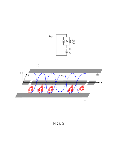
Figure 5: (a) (Color online) Schematic diagram of a superconducting charge qubit. Here, $E_{J0}$ is the Josephson coupling energy, $C_{J0}$ is the Josephson capacitance, $C_{g}$ is the gate capacitance, $V_{g}$ is the gate voltage, and $\Phi$ is the external magnetic flux applied to the SQUID loop through a control line (not shown). (b) $N$ superconducting qubits (red squares) are placed into a (grey) quasi-one dimensional transmission line resonator. Each qubit is placed at an antinode of the electric field, yielding a strong coupling between the qubit and the resonator mode. The two blue curves represent the standing-wave electric field, along the $y$-direction. A subset of qubits from the $N$ qubits, selected for the gate, are coupled to each other via the resonator mode; while the remaining qubits, which are not controlled by the gate, are decoupled from the resonator mode by setting their $\Phi=\Phi_{0}/2,~{}V_{g}^{\mathrm{dc}}=e/C_{g},$ and $V_{g}^{\mathrm{ac}}=0$ to have their free Hamiltonian equal to zero.

Let us now consider $N$ identical charge qubits coupled to a single-mode resonator [Fig. 5(b)]. One can select a subset of qubits for the gate, while the remaining qubits, which are not controlled by the gate, are decoupled from the resonator mode by setting their $\Phi=\Phi_{0}/2,~{}V_{g}^{\mathrm{dc}}=e/C_{g},$ and $V_{g}^{\mathrm{ac}}=0$ to have their free Hamiltonian equal to zero. Without loss of generality, we assume that the set of qubits selected for the gate are the $\left(n+1\right)$ qubits labelled by 1, 2, …, and $n+1$ (here, $1<n<N$). From the discussion above, it can be seen that the Hamiltonian for the $\left(n+1\right)$ qubits and the resonator mode is

$$H = E_{z}\widetilde{S}_{z}-E_{J}\left(\Phi\right)\widetilde{S}_{x}+\hbar\omega_{c}a^{\dagger}a$$ (45)

$$+\hbar\Omega\cos\left(\omega t+\varphi\right)\widetilde{S}_{z}+\hbar g\left(a+a^{\dagger}\right)\widetilde{S}_{z},$$

where $\widetilde{S}_{z}=\sum_{j=1}^{n+1}\widetilde{\sigma}_{z,j}$ and $\widetilde{S}_{x}=\sum_{j=1}^{n+1}\widetilde{\sigma}_{x,j},$ with $\widetilde{\sigma}_{z,j}=\left|+_{j}\right\rangle\left\langle+_{j}\right|-\left|-_{j}\right\rangle\left\langle-_{j}\right|$ and $\widetilde{\sigma}_{x,j}=\left|+_{j}\right\rangle\left\langle-_{j}\right|+\left|-_{j}\right\rangle\left\langle+_{j}\right|.$ By setting $E_{z}=0$ (i.e., $n_{g}^{\mathrm{dc}}=1/2$) for each qubit and defining $\omega_{0}/2=E_{J}\left(\Phi\right)/\hbar$, the Hamiltonian (45) reduces to

$$H = -\frac{\hbar\omega_{0}}{2}\widetilde{S}_{x}+\hbar\omega_{c}a^{\dagger}a$$ (46)

$$+\hbar\Omega\cos\left(\omega t+\varphi\right)\widetilde{S}_{z}+\hbar g\left(a+a^{\dagger}\right)\widetilde{S}_{z}.$$

Define now the new qubit basis $\left|0_{j}\right\rangle=\left(\left|+_{j}\right\rangle+\left|-_{j}\right\rangle\right)/\sqrt{2}$ and $\left|1_{j}\right\rangle=\left(\left|+_{j}\right\rangle-\left|-_{j}\right\rangle\right)/\sqrt{2},$ i.e., perform a basis transformation from the $\widetilde{\sigma}_{z,j}$ basis $\left\{\left|+_{j}\right\rangle,\left|-_{j}\right\rangle\right\}$ to the $\sigma_{z,j}$ basis $\left\{\left|0_{j}\right\rangle,\left|1_{j}\right\rangle\right\}$ for the $j$th qubit. Thus, in the new basis, the Hamiltonian (46) becomes

$$H=H_{0}+H_{1}+H_{2},$$ (47)

where

$$H_{0} = -\frac{\hbar\omega_{0}}{2}S_{z}+\hbar\omega_{c}a^{\dagger}a,$$ (48)

$$H_{1} = \hbar\Omega\cos\left(\omega t+\varphi\right)S_{x},$$ (49)

$$H_{2} = \hbar g\left(a+a^{\dagger}\right)S_{x}.$$ (50)

Here, the collective operators $S_{z}$ and $S_{x}$ are the same as those given in Eq. (7) and Eq. (12). In the interaction picture with respect to $H_{0},$ we obtain from Eqs. (49) and (50) (under the rotating-wave approximation and assuming $\omega=\omega_{0}$)

$$H_{1} = \frac{\hbar\Omega}{2}\left(e^{i\varphi}S_{-}+e^{-i\varphi}S_{+}\right),$$ (51)

$$H_{2} = \hbar g\left(e^{i\delta t}aS_{+}+e^{-i\delta t}a^{\dagger}S_{-}\right),$$ (52)

where the collective operators $S_{-}$ and $S_{+}$ are the same as those given in Eq. (7), and $\delta$ $=\omega_{0}-\omega_{c}<0.$

Note that $\omega_{0}=4E_{J0}\cos\left(\pi\Phi/\Phi_{0}\right)/\hbar$. Hence, the qubit transition frequency $\omega_{0}$ can be adjusted by changing the external magnetic flux $\Phi$ applied to the SQUID loop of the charge qubit.

We now turn off the ac gate voltage applied to the charge qubit $1$ (i.e., setting $V_{g}^{\mathrm{ac}}=0$ for the charge qubit $1$) and adjust the transition frequency $\omega_{0}$ of the charge qubit $1$ to have qubit $1$ decoupled (largely detuned) from the resonator mode. In this way, we can drop the terms corresponding to the index $j=1$ from the collective operators $S_{+}=\sum_{j=1}^{n+1}\sigma_{j}^{+}$ and $S_{-}=\sum_{j=1}^{n+1}\sigma_{j}^{-}$ involved in Hamiltonians (51) and (52). In addition, adjust either the transition frequency $\omega_{0}$ of qubits ($2,3,...,n+1$) or the resonator frequency $\omega_{c}$, to achieve a detuning $\delta^{\prime}=\omega_{0}-\omega_{c}>0,$ and set an ac gate voltage $V_{g}^{\mathrm{ac}}=V_{0}^{\prime}\cos\left(\omega t+\varphi\right)$ (with $\omega=\omega_{0}$) for each of qubits ($2,3,...,n+1$). The Rabi frequency $\Omega^{\prime}$ for each ac gate voltage (i.e., the pulse) is given by $\Omega^{\prime}=2E_{c}C_{g}V_{0}^{\prime}/\left(\hbar e\right).$ After replacing $\Omega,$ $\delta,$ and $g,$ with $\Omega^{\prime},$ $\delta^{\prime},$ and $g^{\prime}$, respectively; we can obtain from Eqs. (51) and (52)

$$H_{1}^{\prime} = \frac{\hbar\Omega^{\prime}}{2}\left(e^{i\varphi}S_{-}^{\prime}+e^{-i\varphi}S_{+}^{\prime}\right),$$ (53)

$$H_{2}^{\prime} = \hbar g^{\prime}\left(e^{i\delta^{\prime}t}aS_{+}^{\prime}+e^{-i\delta^{\prime}t}a^{\dagger}S_{-}^{\prime}\right),$$ (54)

which are written in the interaction picture with respect to $H_{0}$ in Eq. (48). Here, the collective operators $S_{-}^{\prime}$ and $S_{+}^{\prime}$ are the same as those given in Eq. (22).

One can see that the four Hamiltonians (51-54) obtained here have the same forms as the Hamiltonians (8), (9), (20), and (21), respectively. Hence, the NTCP gate can be implemented with charge qubits coupled to a resonator. A more detailed discussion on this is given in the next subsection.

B. NTCP gates with charge qubits coupled to a resonator

Following the first method introduced in the previous section (see section IV.A), we now discuss how to implement the NTCP gate with $(n+1)$ charge qubits ($1,$ $2,$ $...,$ $n+1$), coupled to a superconducting resonator. To begin with, it should be mentioned that: (a) for each step of the operations, the dc gate voltage $V_{g}^{\mathrm{dc}}$ for each one of qubits ($1,$ $2,$ $...,$ $n+1$) is set by $V_{g}^{\mathrm{dc}}=e/C_{g},$ such that $E_{z}=0$ for each qubit; and (b) the resonator mode frequency $\omega_{c}$ is  fixed during the entire operation. The three-step operations for the gate realization are illustrated in Fig. 6.

Figure 6: Change of the qubit transition frequency $\omega_{0}$ and the ac gate-voltage frequency $\omega$ during a three-step NTCP gate with charge qubits coupled to a resonator. The three figures on the left side correspond to the charge control qubit $1,$ which (from top to bottom) are for the operations of step (i), step (ii), and step (iii), respectively. The three figures on the right side correspond to the charge target qubits ($2,3,...,n+1$), (from top to bottom) for the operations of step (i), step (ii), and step (iii), respectively. In each figure, the two horizontal solid lines represent the qubit levels $\left|0\right\rangle$ and $\left|1\right\rangle$; $\omega_{c}$ is the resonator mode frequency; $\omega_{0}$ is the qubit transition frequency; $\omega$ is the frequency of the ac gate voltage $V_{g}^{\mathrm{ac}}$ (i.e., the pulse); and $\Omega\left(V_{0}\right)$, $\Omega^{\prime}\left(V_{0}^{\prime}\right),$ $\Omega_{1}\left(V_{0}^{1}\right)$, or $\Omega_{r}\left(V_{0}^{\mathrm{r}}\right)$ is the function of the amplitude $V_{0},$ $V_{0}^{\prime},$ $V_{0}^{1},$ or $V_{0}^{r}$ of the ac gate voltage, which can be adjusted by changing the ac gate-voltage amplitude; and each circle with a symbol $\sim$ represents an ac gate voltage. In (b), the ac gate voltage for qubit $1$ is set to zero (i.e., $V_{g}^{\mathrm{ac}}=0$). In addition, $\delta$ and $\delta^{\prime}$ are the small detunings of the resonator mode with the $\left|0\right\rangle\leftrightarrow\left|1\right\rangle$ transition, which are given by $\delta=\omega_{0}-\omega_{c}<0$ and $\delta^{\prime}=\omega_{0}-\omega_{c}>0$; while $\Delta=\omega_{0}-\omega_{c}$ represents the large detuning of the resonator mode with the $\left|0\right\rangle\leftrightarrow\left|1\right\rangle$ transition. Note that the resonator mode frequency $\omega_{c}$ is kept fixed during the entire operation, but the qubit transition frequency $\omega_{0}$ is adjusted to achieve a different detuning $\delta,\delta^{\prime}$, or $\Delta$ for each step.

From Fig. 6, it can be seen that there is no need of adjusting the resonator mode frequency $\omega_{c}$. Hence, the procedure here for the gate realization is an extension of the first method introduced above. Note that the three time-evolution operators $U,$ $U^{\prime}$, and $\widetilde{U}$, obtained from each step, are the same as those obtained from each step in subsection IV.A. Therefore, following the same discussion given there, one can easily see that the NTCP gate can be implemented with $\left(n+1\right)$ charge qubits (i.e., the control charge qubit $1,$ as well as the $n$ target charge qubits $2,3,...,$ and $n+1$). Namely, after the three-step process in Fig. 6, a phase flip (i.e., $\left|-\right\rangle\rightarrow-\left|-\right\rangle$) on the state $\left|-\right\rangle$ of each target charge qubit is achieved when the control charge qubit $1$ is initially in the state $\left|-\right\rangle$, but nothing happens to the states $\left|+\right\rangle$ and $\left|-\right\rangle$ of each target charge qubit when the control charge qubit $1$ is initially in the state $\left|+\right\rangle.$

From the above description, one can see that the spin operator $\widetilde{\sigma}_{z}$ is identical to $\sigma_{x}.$ In other words, the states $\left|+\right\rangle$ and $\left|-\right\rangle$ are the eigenstates of both operators $\widetilde{\sigma}_{z}$ and $\sigma_{x}.$ Thus, the NTCP gate (implemented with charge qubits here) is actually performed with respect to the eigenstates $\left|+\right\rangle$ and $\left|-\right\rangle$ of the spin operator $\widetilde{\sigma}_{z}$ (i.e., the two charge states $n=0$ and $n=1$ above, for each qubit).

According to the discussion in subsection IV.A, it can be found that to implement the NTCP gate, the following conditions need to be satisfied: (a) $\Omega\gg g,\delta$ and $\Omega^{\prime}\gg g^{\prime},\delta^{\prime};$ (b) $\Omega_{1}=-ng^{2}/\delta+\Omega$ and $\Omega_{r}=-g^{2}/\delta;$ (c) $-\Omega/\delta=\Omega^{\prime}/\delta^{\prime}$ and $-g/\delta=g^{\prime}/\delta^{\prime};$ and (d) $4g^{2}/\delta^{2}=2k+1.$ These conditions can in principle be realized because: (i) The Rabi frequencies $\Omega\left(V_{0}\right),$ $\Omega^{\prime}\left(V_{0}^{\prime}\right),\Omega_{1}\left(V_{0}^{1}\right),$ and $\Omega_{r}\left(V_{0}^{\mathrm{r}}\right)$ are respectively functions of the amplitudes $V_{0},V_{0}^{\prime}$, $V_{0}^{1},$ and $V_{0}^{\mathrm{r}}$ of the ac gate voltages, which can be adjusted by changing the amplitudes of the ac gate voltages; and (ii) The detunings $\delta$ and $\delta^{\prime}$ can be adjusted by changing the qubit transition frequency $\omega_{0}.$

Note that $n_{g}^{\mathrm{dc}}=1/2$ (i.e., $E_{z}=0$) was set for each qubit during the entire operation. We now give some discussion on the deviation from the degeneracy point $n_{g}^{\mathrm{dc}}=1/2$ for each one of the qubits ($1,~{}2,~{}...,~{}n+1$), during each step shown in Fig. (6).

(a) For each one of the qubits ($1,~{}2,~{}...,~{}n+1$) in step (i), we have, from Eq. (42), that

$$n_{g}=n_{g}^{\mathrm{dc}}+n_{0}^{\mathrm{ac}}\cos\left(\omega t+\varphi\right)+n_{0}^{\mathrm{qu}}(a+a^{\dagger}),$$ (55)

where

$$n_{0}^{\mathrm{ac}} = C_{g}V_{0}/\left(2e\right)=\hbar\Omega/\left(4E_{c}\right),$$

$$n_{0}^{\mathrm{qu}} = C_{g}V_{0}^{\mathrm{qu}}/\left(2e\right)=\hbar g/\left(4E_{c}\right).$$

Therefore, the maximal deviation from the degeneracy point for each one of the qubits ($1,~{}2,~{}...,$ $n+1$) in step (i) is

$$\varepsilon_{0}=\left|n_{g}^{\mathrm{dc}}+n_{0}^{\mathrm{ac}}+n_{0}^{\mathrm{qu}}-1/2\right|=\hbar\left(\Omega+g\right)/\left(4E_{c}\right).$$ (56)

(b) Similarly, one can find that the maximal deviation from the degeneracy point for qubits ($2,3,...,n+1$) in step (ii) is

$$\varepsilon_{1}=\hbar\left(\Omega^{\prime}+g^{\prime}\right)/\left(4E_{c}\right).$$ (57)

Note that the deviation from the degeneracy point for qubit $1$ is smaller than $\varepsilon_{1}$ since $V_{g}^{\mathrm{ac}}=0$ and thus $n_{0}^{\mathrm{ac}}=0$ for qubit $1.$

(d) For step (iii), we have $n_{0}^{\mathrm{ac}}=\hbar\Omega_{1}/\left(4E_{c}\right)$ for qubit $1,$ $n_{0}^{\mathrm{ac}}=\hbar\Omega_{r}/\left(4E_{c}\right)$ for qubits ($2,3,...,n+1$), and $n_{0}^{\mathrm{qu}}=0.$ Thus, it is easy to see that the maximal deviation from the degeneracy point for qubit $1$ is

$$\varepsilon_{2}=\hbar\Omega_{1}/\left(4E_{c}\right),$$ (58)

and the deviation from the degeneracy point for qubits ($2,3,...,n+1$) is

$$\varepsilon_{3}=\hbar\Omega_{r}/\left(4E_{c}\right).$$ (59)

In the above, we have discussed how to realize the NTCP gate with superconducting charge qubits coupled to a resonator. Note that the proposal here can implement multi-qubit gates, while previous proposals (e.g.,[49-51]) using superconducting qubits are limited to two-qubit gates.

C. Possible experimental implementation

In this section we discuss some issues which are relevant for future experimental implementation of our proposal. For the method to work: (a) The conditions for the Rabi frequencies $\Omega,$ $\Omega^{\prime},$ $\Omega_{1},$ and $\Omega_{r},$ which were discussed above, need to be met; (b) The total operation time

$$t_{\mathrm{op}}=2\tau+\tau^{\prime}=4\pi/\left|\delta\right|+2\pi/\delta^{\prime}$$ (60)

should be much shorter than the energy relaxation time $T_{1}$ and the dephasing time $T_{2}$ of the qubit and the lifetime of the resonator mode $\kappa^{-1}=Q/\omega_{c},$ where $Q$ is the (loaded) quality factor of the resonator; (c) The deviations $\varepsilon_{0},$ $\varepsilon_{1},$ $\varepsilon_{2},$ and $\varepsilon_{3}$ from the degeneracy point need to be small numbers to have the qubits working near the degeneracy point, such that the qubits are less affected by the low-frequency charge noises [52,53]; and (d) The direct coupling between SQUIDs needs to be negligible, since this interaction is not intended. It is noted that the direct interaction between SQUIDs can be made negligibly small as long as $D\gg d$ (where $D$ is the distance between the two nearest SQUIDs and $d$ is the linear dimension of each SQUID).

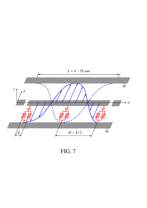
Figure 7: (Color online) Proposed setup for three qubits (red squares) and a (grey) standing-wave quasi-one dimensional coplanar waveguide cavity (not drawn to scale). Each qubit is placed at an antinode of the electric field. The two blue curves represent the standing-wave electric field, along the $y$-direction. $V_{g}$ is the gate voltage, $D$ is the distance between any two nearest SQUID loops, and $d$ is the linear dimension of each SQUID loop.

Table 1: Possible experimental parameters of a charge qubit [8,54-56]. Here, $\Omega_{p}$ is the typical Rabi frequency available in experiments, and $\Delta\nu_{0}$ is the experimentally tuning range of the qubit frequency.

For the sake of definitiveness, let us consider the experimental feasibility of implementing a two-target-qubit controlled phase gate using superconducting charge qubits with parameters listed in Table I [8,54-56]. Note that in a recent experiment, coupling three superconducting qubits with a transmission line resonator has been demonstrated [57]. For a superconducting one dimensional standing-wave CPW (coplanar waveguide) transmission line resonator and each qubit placed at an antinode of the resonator mode (Fig. 7), the amplitude of the quantum part of the gate voltage is given by [48]

$$V_{0}^{\mathrm{qu}}=\left(\hbar\omega_{c}\right)^{1/2}\left(Lc_{0}\right)^{-1/2},$$ (61)

where $L$ is the length of the resonator and $c_{0}$ is the capacitance per unit length of the resonator. Therefore, the coupling constant $g$ is given by

$$g=2E_{c}C_{g}\left(\hbar e\right)^{-1}\left(\hbar\omega_{c}\right)^{1/2}\left(Lc_{0}\right)^{-1/2},$$ (62)

showing that $g$ does not depend on the detuning $\delta$. Therefore, we have $g=g^{\prime}$, for which the above condition $-\Omega/\delta=\Omega^{\prime}/\delta^{\prime}$ and $-g/\delta=g^{\prime}/\delta^{\prime}$ simply turns to the $\Omega=\Omega^{\prime}$ and $-\delta=\delta^{\prime}.$ For superconducting charge qubits with parameters given in Table I, and a resonator with the parameters listed in Table II [36,57-59], a simple calculation gives $g/2\pi\sim 22$ MHz, which is available in experiments (see, e.g., [58]). With a choice of $-\delta=\delta^{\prime}=2g$ [corresponding to $k=0$ in Eq. (36)], the total operation time $t_{\mathrm{op}}$ would be $\sim 68$ ns, which is much shorter than the dephasing time $T_{2}$ and $\kappa^{-1}\sim 794$ ns for a resonator with $Q=10^{5}$. Note that a superconducting CPW resonator with a quality factor of $Q>10^{6}$ has been experimentally demonstrated [59].

Table 2: Possible experimental parameters of a resonator [36,57-59]. Here, $\Delta\nu_{c}$ is the experimentally tuning range of the resonator frequency.

Based on $\Omega=$ $\Omega^{\prime}$, $\Omega_{1}=4\lambda n+\Omega,$ and $\Omega_{r}=4\lambda$ ($n=2$ for a two-target-qubit gate), we have $\Omega^{\prime}/\left(2\pi\right)\sim 330$ MHz, $\Omega_{1}/\left(2\pi\right)\sim 352$ MHz, and $\Omega_{r}/\left(2\pi\right)\sim 11$ MHz for a choice of $\Omega\sim 15g,$ i.e., $\Omega/\left(2\pi\right)\sim 330$ MHz. For the Rabi frequencies given here, we obtain $\varepsilon_{0}=$ $\varepsilon_{1}\sim 2.75\times 10^{-3},$ $\varepsilon_{2}\sim 2.75\times 10^{-3},$ and $\varepsilon_{3}\sim 8.59\times 10^{-5}$ for a qubit-cavity system with the above parameters. Therefore, the conditions for the qubits to work near the degeneracy point are well satisfied.

Finally, for a resonator with $\omega_{c}/\left(2\pi\right)=10$ GHz, the wavelength of the resonator mode is $\lambda\sim 10$ mm. For the charge qubits placed in a resonator as shown in Fig. 7, the distance between any two nearest SQUIDs is $D\sim\lambda/2\sim 5$ mm. Hence, the ratio $D/d$ would be $\sim 250$ for $d=20\mu$m. Note that the dipole field generated by the current in each SQUID ring at a distance $r\gg d$ decreases as $r^{-3}$. Thus, the condition of negligible direct coupling between SQUIDs is well satisfied.

Note that because of $\omega_{0}=4E_{J0}\cos\left(\pi\Phi/\Phi_{0}\right)/\hbar,$ it can be found that for charge qubits with the parameters given in Table I, the transition frequency $\nu_{0}=\omega_{0}/2\pi$ of each qubit varies from $\nu_{0}=0$ GHz for $\Phi/\Phi_{0}=1/2$ to $\nu_{0}=20$ GHz for $\Phi=0$. Therefore, the choice of the resonator frequency above is reasonable. For the choice of $-\delta=\delta^{\prime}=2g$ above, the qubit transition frequency $\nu_{0}$ would be $\sim 9.956$ GHz for the detuning $\delta=-2g$ while $\sim 10.044$ GHz for the detuning $\delta^{\prime}=2g.$

The above analysis shows that the realization of a two-target-qubit controlled phase gate is possible using superconducting charge qubits and a resonator. We remark that a quantum-controlled phase gate with a larger number of target qubits can in principle be obtained by increasing the length of the resonator since the total operation time $t_{\mathrm{op}}$ is independent of the number of target qubits $n.$

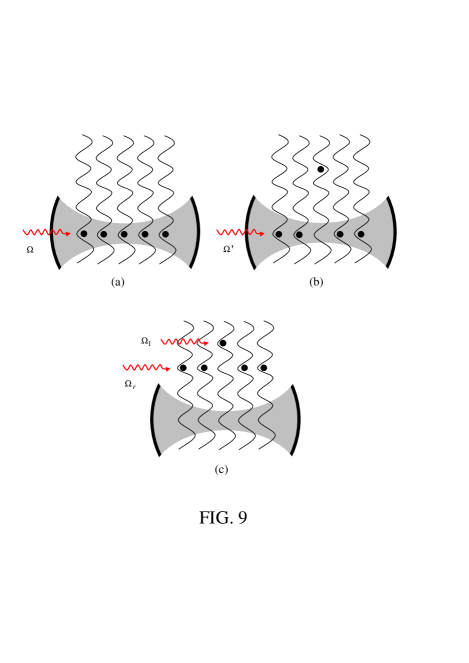
Figure 8: (Color online) Proposed set-up for an $n$-target-qubit control phase (NTCP) gate with ($n+1$) identical neutral atoms and a cavity. For simplicity, only five atoms are drawn here. Each atom can be either loaded into the cavity or moved out of the cavity by one-dimensional translating optical lattices [20,45,46]. The atom in the middle represents atom 1 (the control qubit), while the remaining atoms play the role of target qubits.

VI. NTCP GATE WITH ATOMS USING ONE CAVITY

Consider $\left(n+1\right)$ identical two-level atoms ($1,2,...,n+1$). The two levels of each atom are labelled by $\left|0\right\rangle$ and $\left|1\right\rangle.$ The transition frequency of each atom is denoted as $\omega_{0}.$ Each atom is trapped in the periodic potential of a one-dimensional optical lattice and can be loaded into or moved out of the cavity by translating the optical lattice [20,45,46]. The NTCP gate can be realized using a procedure illustrated in Fig. 8. The operations shown in Fig. 8 are as follows:

$\bullet$ Figure 8(a): Move atoms ($1,2,...,n+1$) into the cavity and then apply a classical pulse (with an initial phase $\varphi=\pi$ and frequency $\omega=\omega_{0}$) to the atoms. The cavity mode is coupled to the $\left|0\right\rangle\rightarrow$ $\left|1\right\rangle$ transition of each atom, with a detuning $\delta=\omega_{0}-\omega_{c}<0$, which can be achieved by prior adjustment of the cavity mode frequency [35]. The time-evolution operator for this operation is the $U$ in Eq. (19) for an interaction time $\tau=-2\pi/\delta.$

$\bullet$ Figure 8(b): Move atoms ($1,2,...,n+1$) out of the cavity and then adjust the cavity mode frequency. After adjusting the cavity mode frequency, move atoms ($2,3,...,n+1$) back into the cavity and then apply a classical pulse (with $\varphi=0$ and $\omega=\omega_{0}$) to them. The cavity mode frequency is adjusted such that the cavity mode is coupled to the $\left|0\right\rangle\rightarrow$ $\left|1\right\rangle$ transition of atoms ($2,3,...,n+1$), with a detuning $\delta^{\prime}=\omega_{0}-\omega_{c}>0$. The time-evolution operator for this operation is the $U^{\prime}$ in Eq. (26) for an interaction time $\tau^{\prime}=2\pi/\delta^{\prime}.$

$\bullet$ Figure 8(c): Move atoms ($2,3,...,n+1$) out of the cavity. Apply a classical pulse (with $\varphi=0$ and $\omega=\omega_{0}$) to the control atom $1$ and a classical pulse (with the same initial phase and frequency) to the target atoms ($2,3,...,n+1$). The Rabi frequency for the pulse applied to atom $1$ is $\Omega_{1}$, while the Rabi frequency for the pulses applied to atoms ($2,3,...,n+1$) is $\Omega_{r}.$ This operation is described by the operator $\widetilde{U}$ in Eq. (28) for an interaction time $\tau$.

The three time-evolution operators $U,$ $U^{\prime}$, and $\widetilde{U}$ here are the same as those obtained from each step in subsection IV.A. Therefore, as long as the conditions given in subsection IV.A are met, an NTCP gate described by Eq. (39) is implemented with the $\left(n+1\right)$ atoms. Namely, after the operations shown in Fig. 8, $n$ two-qubit controlled phase gates, each described by the unitary transformation in Eq. (1), are performed on the atom pairs ($1,2$), ($1,3$),…, and ($1,n+1$), respectively. Note that each pair contains the same control qubit (atom $1$) but a different target qubit (atom $2,3,...,$ or $n+1$).

As shown above, the present scheme for implementing the NTCP gate with atoms has the following features:

(a) No adjustment of the level spacings for each atom is required during the entire operation;

(b) Only one cavity is required;

(c) The cavity mode can be initially in an arbitrary state; and

(d) The operation time does not depend on the number of atoms.

For our scheme to work, the total operation time $t_{\mathrm{op}}=\tau+\tau^{\prime}+\tau_{\mathrm{a}}+4\tau_{\mathrm{m}}$ should be much smaller than the cavity decay time $\kappa^{-1}$, so that the cavity dissipation is negligible. Here, $\tau_{\mathrm{a}}$ is the typical time required for adjusting the cavity mode frequency during step (ii) above, and $\tau_{\mathrm{m}}$ is the typical time required for moving atoms into or out of the cavity. In addition, the $t_{\mathrm{op}}$ needs to be much smaller than the energy relaxation time of level $\left|1\right\rangle$, such that the decoherence induced due to the spontaneous decay of the level $\left|1\right\rangle$ is negligible. In principle, these conditions can be satisfied by choosing a cavity with a high quality factor $Q$ and atoms with a sufficiently long energy relaxation time.

To investigate the experimental feasibility of this proposal, let us consider Rydberg atoms with principal quantum numbers 50 and 51 (respectively corresponding to the levels $\left|0\right\rangle$ and $\left|1\right\rangle$). The $\left|0\right\rangle\leftrightarrow\left|1\right\rangle$ transition frequency is $\omega_{0}/2\pi\sim 51.1$ GHz, the energy relaxation time of the level $\left|1\right\rangle$ is $T_{r}\sim 3\times 10^{-2}$ s, and the coupling constant is $g=2\pi\times 50$ KHz [35,60]. Now set $-\delta=\delta^{\prime}=2g$, and assume $g\sim g^{\prime}$. With the choice of these parameters, the time needed for the entire operation is $t_{\mathrm{op}}\sim$ 65 $\mu$s for $\tau_{\mathrm{a}}=\tau_{\mathrm{m}}\sim 1$ $\mu$s, which is much shorter than $T_{r}$. The cavity mode frequency is $\omega_{c}/2\pi\sim 51.2$ GHz for the negative qubit detuning $\delta=-2g$ while $\sim 51$ GHz for the positive qubit detuning $\delta^{\prime}=2g.$ To estimate the lifetime of the cavity photon, we here consider the conservative case of a larger cavity frequency $\omega_{c}/2\pi\sim 51.2$ GHz, for which the lifetime of the cavity photon is $T_{c}=Q/\omega_{c}\sim 622$ $\mu$s for a cavity with $Q=2\times 10^{8}$, which is much larger than the total operation time $t_{\mathrm{op}}.$ Note that cavities with a high $Q\sim 10^{10}$ have been demonstrated in experiments [61]. Thus, the present proposal might be realizable using current cavity QED setups.

VII. CONCLUSIONS

We have presented two different methods for the proposed NTCP gate implementation. The two methods are quite general, which can be applied to physical systems such as trapped atoms, quantum dots, and superconducting qubits. For the two methods, we have provided guidelines on how to protect multi-level qubits from leaking out of the computational subspace.

Using a concrete example, we have shown how to apply the first method to implement the NTCP gate with superconducting qubits coupled to a resonator. In addition, we have discussed the experimental feasibility of performing a two-target-qubit controlled phase gate with superconducting qubits coupled to a one-dimensional transmission line resonator. Our analysis shows that the realization of this gate is possible within current technologies. How well this gate would work in light of experimental errors should be further investigated elsewhere for each particular set-up or implementation. This is beyond the scope of this theoretical work.

We have shown how to extend the second method to implement the NTCP gate with trapped atomic qubits by using one cavity. Interestingly, as shown above, there is no need to adjust the level spacings of atoms during the entire operation, and decoupling of atoms with the cavity can be easily achieved by just moving atoms out of the cavity.

In summary, we have presented a general proposal to implement a NTCP gate with qubits in a cavity or coupled to a resonator. As shown above, the present proposal has the following features: (i) The $n$ two-qubit CP gates involved in the NTCP gate can be simultaneously performed; (ii) The operation time required for the gate implementation is independent of the number of the target qubits, thus it does not increase with the number of qubits; (iii) The gate is insensitive to the initial state of the cavity mode, therefore no preparation for a specified initial state of the cavity mode is needed; (iv) No measurement on the qubits or the cavity mode is needed and thus the operation is simplified, (v) The gate realization requires only three steps of operations.

ACKNOWLEDGMENTS

FN and CPY acknowledge partial support from the National Security Agency (NSA), Laboratory for Physical Sciences (LPS), (U.S.) Army Research Office (USARO), National Science Foundation (NSF) under Grant No. 0726909, and JSPS-RFBR under Contract No. 06-02-91200. YXL is supported by the National Natural Science Foundation of China under Grant Numbers 10975080 and 60836001.

APPENDIX: HOW TO PROTECT QUBITS FROM LEAKING TO HIGHER ENERGY LEVELS

Let us now discuss how to protect qubits from leaking out of the computational subspace in the presence of more qubit levels. Generally speaking, we need to consider two situations, which are here denoted as cases $L$ and $S$. For case $L$, the level spacing between the level $\left|1\right\rangle$ and the level $\left|2\right\rangle$ (the first level above $\left|1\right\rangle$) is larger than the level spacing between the levels $\left|0\right\rangle$ and $\left|1\right\rangle.$ Namely, for case $L$, $\left(E_{2}-E_{1}\right)>\left(E_{1}-E_{0}\right),$ where $E_{0},$ $E_{1},$ and $E_{2}$ are the energy eigenvalues of the levels $\left|0\right\rangle,\left|1\right\rangle,$ and $\left|2\right\rangle.$ For case $S$, the level spacing between the levels $\left|1\right\rangle$ and $\left|2\right\rangle$ is smaller than that between the levels $\left|0\right\rangle$ and $\left|1\right\rangle.$ Namely, $\left(E_{2}-E_{1}\right)<\left(E_{1}-E_{0}\right).$ For solid-state qubits, case $L$ exists for superconducting charge qubits and flux qubits [31]; while case $S$ can be applied to superconducting phase qubits [33]. For atomic qubits, the level structures for both cases $L$ and $S$ are available.

Here and below, we define $\Delta_{2}=\left(E_{2}-E_{1}\right)/\hbar-\omega_{c}$, $\Delta_{3}=\left(E_{3}-E_{1}\right)/\hbar-\omega_{c}$, and $\Delta_{a}=\left(E_{a}-E_{1}\right)/\hbar-\omega_{c}$, as the large detuning of the cavity mode with the $\left|1\right\rangle\leftrightarrow\left|2\right\rangle$ transition, the large detuning of the cavity mode with the $\left|1\right\rangle\leftrightarrow\left|3\right\rangle$ transition, and the large detuning of the cavity mode with the $\left|1\right\rangle\leftrightarrow\left|a\right\rangle$ transition, respectively. $E_{a}$ is the energy eigenvalue of level $\left|a\right\rangle$.

A. Case $L$:  $\left(E_{2}-E_{1}\right)>\left(E_{1}-E_{0}\right)$

For case $L,$ let us consider Fig. 9(a), where the dashed line falls within the range between the levels $\left|1\right\rangle$ and $\left|2\right\rangle$ when the cavity mode is slightly detuned from the $\left|0\right\rangle\leftrightarrow\left|1\right\rangle$ transition. Therefore, a large detuning $\Delta_{2}$ is needed to avoid the transition from the level $\left|1\right\rangle$ to the level $\left|2\right\rangle$. Note also that as long as this large detuning is met, no transition from level $\left|1\right\rangle$ to the higher energy level above the level $\left|2\right\rangle$ happens. To explain this, let us consider an arbitrary level $\left|a\right\rangle$ above level $\left|2\right\rangle$ [Fig. 9(a)]. Since the detuning $\Delta_{a}$ is larger than the detuning $\Delta_{2}$, then the large detuning regime for $\Delta_{a}$ is automatically satisfied when $\Delta_{2}$ is large. As a result, the transition from the level $\left|1\right\rangle$ to the level $\left|a\right\rangle$ will not be induced by the cavity mode. In addition, the excitation of the level $\left|a\right\rangle,$ induced due to its coupling to the level $\left|2\right\rangle$ via the cavity mode, does not occur when the level $\left|2\right\rangle$ is unpopulated. Hence, as long as the large detuning $\Delta_{2}$ is satisfied, no level above $\left|1\right\rangle$ will be populated and therefore the leak out of the computational subspace is suppressed.

Figure 9: Large detuning of the cavity mode with the transition between energy levels. Figure (a) corresponds to the case $L$, while figure (b) corresponds to case $S.$ The dots above level $\left|2\right\rangle$ in (a) and level $\left|3\right\rangle$ in (b) represent other energy levels.

B. Case $S$:  $\left(E_{2}-E_{1}\right)<\left(E_{1}-E_{0}\right)$

For case $S,$ let us consider Fig. 9(b), where the dashed line falls within the range between the levels $\left|2\right\rangle$ and $\left|3\right\rangle$, when the cavity mode is slightly detuned from the $\left|0\right\rangle\leftrightarrow\left|1\right\rangle$ transition. This can be achieved, e.g., for superconducting qubits by appropriately choosing the device parameters and/or adjusting the external parameters to control the level structures. From Fig. 9(b), it can be seen that a large detuning $\Delta_{2}$ and a large detuning $\Delta_{3}$ are needed to avoid the transition from the level $\left|1\right\rangle$ to the level $\left|2\right\rangle$ or the level $\left|3\right\rangle$. Note also that as long as these two large detunings are met, no transition from the level $\left|1\right\rangle$ to the higher energy level above the level $\left|3\right\rangle$ occurs. To understand this, let us consider an arbitrary level $\left|a\right\rangle$ above $\left|3\right\rangle$ [Fig. 9(b)]. Note that the detuning $\Delta_{a}$ is larger than the detuning $\Delta_{3}$. Therefore, the large detuning regime for $\Delta_{a}$ is automatically satisfied when the cavity mode is largely detuned from the $\left|1\right\rangle$ $\leftrightarrow\left|3\right\rangle$ transition. As a result, the transition from level $\left|1\right\rangle$ to level $\left|a\right\rangle$ will not be induced by the cavity mode. In addition, the excitation of the level $\left|a\right\rangle$, caused due to its coupling to the level $\left|2\right\rangle$ or $\left|3\right\rangle$ via the cavity mode, will not happen when levels $\left|2\right\rangle$ and $\left|3\right\rangle$ are unpopulated. Hence, as long as the large detunings $\Delta_{2}$ and $\Delta_{3}$ are met, the levels above $\left|1\right\rangle$ will not be excited by the cavity mode.

We now give a quantitative analysis on the effect of the finite detuning of the qubit frequencies with the cavity mode. For simplicity, we consider the case where the cavity mode is in a single photon state and the qubit is in the state $\left|1\right\rangle.$ It is estimated that the occupation probability $p_{2}$ for level $\left|2\right\rangle$ and the occupation probability $p_{3}$ for level $\left|3\right\rangle$ (induced by the photon) would be on the order of $4g_{12}^{2}/\left(4g_{12}^{2}+\Delta_{2}^{2}\right)$ and $4g_{13}^{2}/\left(4g_{13}^{2}+\Delta_{3}^{2}\right),$ respectively. Here, $g_{12}$ is the coupling constant between the cavity mode and the $\left|1\right\rangle\leftrightarrow\left|2\right\rangle$ transition, while $g_{13}$ is the coupling constant between the cavity mode and the $\left|1\right\rangle\leftrightarrow\left|3\right\rangle$ transition. With a choice of $\Delta_{2}=10g_{12}$ and $\Delta_{3}=10g_{13},$ we have $p_{2},$ $p_{3}\sim 0.04,$ which can be further reduced by increasing the detuning $\Delta_{2}$ or $\Delta_{3}.$ Therefore, the population probability of the level $\left|2\right\rangle$ or $\left|3\right\rangle$ of the qubit can be made negligible by choosing the detuning appropriately.

References

(1) C. Monroe, D. M. Meekhof, B. E. King, W. M. Itano, and D. J.
Wineland, Phys. Rev. Lett. 75, 4714 (1995).
(2) J. A. Jones, M. Mosca, and R. H. Hansen, Nature (London) 393, 344 (1998).
(3) X. Li, Y. Wu, D. Steel. D. Gammon, T. H. Stievater, D. D.
Katzer, D. Park, C. Piermarocchi, and L. J. Sham, Science 301, 809
(2003).
(4) T. Yamamoto, Yu. A. Pashkin, O. Astafiev, Y. Nakamura, and J.
S. Tsai, Nature (London) 425, 941 (2003).
(5) J. H. Plantenberg, P. C. de Groot, C. J. P. M. Harmans, and J.
E. Mooij, Nature (London) 447, 836 (2007).
(6) R. C. Bialczak, M. Ansmann, M. Hofheinz, E. Lucero, M. Neeley,
A. O’Connell, D. Sank, H. Wang, J. Wenner, M. Steffen, A. Cleland,
and J. Martinis, arXiv:0910.1118.
(7) J. Majer, J. M. Chow, J. M. Gambetta, J. Koch, B. R. Johnson,
J. A. Schreier, L. Frunzio, D. I. Schuster, A. A. Houck, A.
Wallraff, A. Blais, M. H. Devoret, S. M. Girvin, and R. J.
Schoelkopf, Nature (London) 449, 443 (2007).
(8) P. J. Leek, S. Filipp, P. Maurer, M. Baur, R. Bianchetti, J. M. Fink,
M. Göppl, L. Steffen, and A. Wallraff, Phys. Rev. B 79,
180511(R)(2009).
(9) D. I. Schuster, A. Wallraff, A. Blais, L. Frunzio, R.-S. Huang,
J. Majer, S. M. Girvin, and R. J. Schoelkopf, Phys. Rev. Lett.
94, 123602 (2005).
(10) J. Q. You and F. Nori, Phys. Rev. B 68, 064509
(2003).
(11) J. Q. You, J. S. Tsai, and F. Nori, Phys. Rev. B 68,
024510 (2003).
(12) C. P. Yang, S. I. Chu, and S. Han, Phys. Rev. A 67, 042311
(2003).
(13) P. Zhang, Z.D. Wang, J.D. Sun, and C.P. Sun, Phys. Rev. A
71, 042301 (2005).
(14) S. L. Zhu, Z. D. Wang, and P. Zanardi, Phys. Rev. Lett. 94, 100502
(2005).
(15) Z. B. Feng, Phys. Rev. A 78, 032325 (2008).
(16) T. Monz, K. Kim, W. Hänsel, M. Riebe, A. S. Villar, P.
Schindler, M. Chwalla, M. Hennrich, and R. Blatt, Phys. Rev. Lett. 102, 040501 (2009).
(17) A. Barenco, C. H. Bennett, R. Cleve, D. P. DiVincenzo, N.
Margolus, P. Shor, T. Sleator, J. A. Smolin, and H. Weinfurter, Phys. Rev. A
52, 3457 (1995).
(18) M. Möttönen, J. J. Vartiainen, V. Bergholm, and M. M.
Salomaa, Phys. Rev. Lett. 93, 130502 (2004).
(19) X. Wang, A. Sørensen, and K. Mølmer, Phys. Rev. Lett.
86, 3907 (2001).
(20) L. M. Duan, B. Wang, and H. J. Kimble, Phys. Rev. A 72,
032333 (2005).
(21) X. M. Lin, Z. W. Zhou, M. Y. Ye, Y. F. Xiao, and G. C. Guo,
Phys. Rev. A 73, 012323 (2006).
(22) C. P. Yang and S. Han, Phys. Rev. A 72, 032311 (2005).
(23) P. W. Shor, in Proceedings of the 35th Annual Symposium
on Foundations of Computer Science, edited by S. Goldwasser (IEEE
Computer Society Press, Los Alamitos, CA, 1994), pp. 124-134.
(24) L. K. Grover, Phys. Rev. Lett. 80, 4329 (1998).
(25) P. W. Shor, Phys. Rev. A 52, R2493 (1995); A. M.
Steane, Phy. Rev. Lett. 77, 793 (1996).
(26) M. Šašura and V. Buzek, Phys. Rev. A 64, 012305
(2001).
(27) F. Gaitan, Quantum Error Correction and Fault
Tolerant Quantum Computing (CRC Press, USA, 2008).
(28) T. Beth and M. Rötteler, Quantum Information, Vol. 173, Ch. 4, p. 96 (Springer, Berlin, 2001).
(29) S. L. Braunstein, V. Buzek, and M. Hillery, Phys. Rev. A 63, 052313 (2001).
(30) Y. Makhlin, G. Schön, and A. Shnirman, Rev. Mod. Phys. 73, 357 (2001).
(31) J. Q. You and F. Nori, Phys. Today 58 (11), 42 (2005).
(32) J. Clarke and F. K. Wilhelm, Nature(London) 453, 1031 (2008).
(33) M. Neeley, M. Ansmann, R. C. Bialczak, M. Hofheinz, N. Katz,
E. Lucero, A. O’Connell, H. Wang, A. N. Cleland, and J. M.
Martinis, Nature Physics 4, 523 (2008); A. M. Zagoskin, S.
Ashhab, J. R. Johansson, and F. Nori, Phys. Rev. Lett. 97,
077001 (2006).
(34) For quantum dots, the level spacings can be changed via
adjusting the external electronic field. For the details, see P.
Pradhan, M. P. Anantram, and K. L. Wang, arXiv:quant-ph/0002006.
(35) M. Brune, E. Hagley, J. Dreyer, X. Maitre, A. Maali, C.
Wunderlich, J. M. Raimond, and S. Haroche, Phys. Rev. Lett. 77, 4887 (1996).
(36) M. Sandberg, C. M. Wilson, F. Persson, T. Bauch, G.
Johansson, V. Shumeiko, T. Duty, and P. Delsing, Appl. Phys. Lett.
92, 203501 (2008).
(37) A. Palacios-Laloy, F. Nguyen, F. Mallet, P. Bertet, D. Vion,
and D. Esteve, J. Low Temp. Phys. 151, 1034 (2008).
(38) J. R. Johansson, G. Johansson, C. M. Wilson, and F.
Nori, Phys. Rev. Lett. 103, 147003 (2009).
(39) J. Q. Liao, Z. R. Gong, L. Zhou, Y. X. Liu, C. P. Sun, and F.
Nori, e-print arXiv:quant-ph/0909.2748. Phys. Rev. A, in press.
(40) S. B. Zheng, Phys. Rev. A 66, 060303(R) (2002).
(41) E. Solano, G. S. Agarwal, and H. Walther, Phys. Rev. Lett.
90, 027903 (2003).
(42) Z. J. Deng, M. Feng, and K. L. Gao, Phys. Rev. A 72,
034306 (2005).
(43) A. Sørensen and K. Mølmer, Phys. Rev. A 62, 022311
(2000).
(44) Y. D. Wang, P. Zhang, D. L. Zhou, and C. P. Sun, Phys. Rev. B
70, 224515 (2004).
(45) A. Beige, D. Braun, B. Tregenna, and P. L. Knight,
Phys. Rev. Lett. 85, 1762 (2000).
(46) J. A. Sauer, K. M. Fortier, M. S. Chang, C. D. Hamley, and M. S.
Chapman, Phys. Rev. A 69, 051804(R) (2004).
(47) M. Hofheinz, H. Wang, M. Ansmann, R. C. Bialczak, E. Lucero,
M. Neeley, A. D. O’Connell, D. Sank, J. Wenner, J. M. Martinis,
and A. N. Cleland, Nature (London) 459, 546 (2009).
(48) A. Blais, R. S. Huang, A. Wallraff, S. M. Girvin, and R. J.
Schoelkopf, Phys. Rev. A 69, 062320 (2004).
(49) J. Q. You, J. S. Tsai, and F. Nori, Phys. Rev. Lett. 89, 197902
(2002).
(50) J. Q. You, Y. Nakamura, and F. Nori, Phys. Rev. B 71, 024532
(2005).
(51) Y. X. Liu, L. F. Wei, J. R. Johansson, J. S. Tsai, and F.
Nori, Phys. Rev. B 76, 144518 (2007).
(52) Y. Nakamura, Y. A. Pashkin, T. Yamamoto, and J. S.
Tsai, Phys. Rev. Lett. 88, 047901 (2002).
(53) D. Vion, A. Aassime, A. Cottet, P. Joyez, H. Pothier, C. Urbina, D. Esteve,
and M. H. Devoret, Science 296, 886 (2002).
(54) O. Astafiev, Y. A. Pashkin, Y. Nakamura, T. Yamamoto, and J.
S. Tsai, Phys. Rev. Lett. 93, 267007 (2004).
(55) A. Wallraff, D. I. Schuster, A. Blais, L. Frunzio, J. Majer,
M. H. Devoret, S. M. Girvin, and R. J. Schoelkopf, Phys. Rev. Lett. 95, 060501 (2005).
(56) M. Baur, S. Filipp, R. Bianchetti, J. M. Fink, M. Göppl, L. Steffen,
P. J. Leek, A. Blais, and A. Wallraff, Phys. Rev. Lett. 102,
243602 (2009).
(57) J. M. Fink, R. Bianchetti, M. Baur, M. Göppl, L. Steffen, S. Filipp,
P. J. Leek, A. Blais, and A. Wallraff, Phys. Rev. Lett. 103,
083601 (2009).
(58) D. I. Schuster, A. A. Houck, J. A. Schreier, A. Wallraff, J.
M. Gambetta, A. Blais, L. Frunzio, J. Majer, B. Johnson, M. H. Devoret, S.
M. Girvin, and R. J. Schoelkopf, Nature (London) 445, 515 (2007).
(59) P. K. Day, H. G. LeDuc, B. A. Mazin, A. Vayonakis, and J.
Zmuidzinas, Nature (London) 425, 817 (2003).
(60) S. Osnaghi, P. Bertet, A. Auffeves, P. Maioli, M. Brune, J. M. Raimond, and S.
Haroche, Phys. Rev. Lett. 87, 037902 (2001).
(61) S. Kuhr, S. Gleyzes, C. Guerlin, J. Bernu, U. B. Hoff, S. Deleglise, S. Osnaghi,
M. Brune, J. M. Raimond, S. Haroche, E. Jacques, P. Bosland, and
B. Visentin, Appl. Phys. Lett. 90, 164101 (2007).