Joint Vertex Degrees in an Inhomogeneous Random Graph Model

K. Lin 111Department of Statistics, University of Oxford, 1 South Parks Road, OXFORD OX1 3TG, UK; email: k.lin@wolfson.oxon.org Β and G. Reinert222Department of Statistics, University of Oxford, 1 South Parks Road, OXFORD OX1 3TG, UK; email: reinert@stats.ox.ac.uk
Abstract

In a random graph, counts for the number of vertices with given degrees will typically be dependent. We show via a multivariate normal and a Poisson process approximation that, for graphs which have independent edges, with a possibly inhomogeneous distribution, only when the degrees are large can we reasonably approximate the joint counts as independent. The proofs are based on Stein’s method and the Stein-Chen method with a new size-biased coupling for such inhomogeneous random graphs, and hence bounds on distributional distance are obtained. Finally we illustrate that apparent (pseudo-) power-law type behaviour can arise in such inhomogeneous networks despite not actually following a power-law degree distribution.

Key words: Stein’s method, size-biased couplings, vertex degrees, inhomogeneous random graphs, power law.
AMS Subject Classification: 60F05, 05C80, 90B15

1 Introduction

It has been observed in many real-world networks that, when plotting the observed number of vertices of degree kπ‘˜\displaystyle k against kπ‘˜\displaystyle k, on a log-log-scale the plots tend to look linear. This so-called scale-free behaviour, see e.g. [7], has motivated the scale-free network model introduced by [1], yielding a probability distribution for the number of vertices of large degree which is scale-free.

Some issues arise when trying to assess the vertex degree distribution from a single network. The log-log scale lends itself to over-interpretation; [16] discusses a good number of pitfalls when trying to test for power law using such plots. Moreover, [19] have shown that when sampling from a scale-free network, the sampled network will not in general be scale-free. In addition, the total number of vertices in the network is fixed, and hence counts for different degrees will be dependent. We shall see in this paper that whether or not the dependence is negligible depends on the size of the degrees under consideration - only when then degrees are large can we reasonably approximate the joint counts as independent. We establish these facts by proving a multivariate normal approximation, with possibly non-diagonal asymptotic covariance matrix, as well as a Poisson process approximation, with independent coordinates. We give bounds for these approximations which depend on the size of the degrees under consideration. Finally we shall illustrate that apparent (pseudo-) power-law type behaviour can arise in networks which are constructed using independent edges, and do not follow a power-law behaviour.

The degree of a vertex is one of the fundamental summaries for random graphs, and hence the degree distribution is a natural object to study. In a general random graph 𝒒nsuperscript𝒒𝑛\displaystyle\mathscr{G}^{n} on a set V𝑉\displaystyle V of n𝑛\displaystyle n vertices, the degree of a vertex v𝑣\displaystyle v, denoted by D​(v)𝐷𝑣\displaystyle D(v), is defined as the number of vertices adjacent to v𝑣\displaystyle v. The most basic model of a random graph is that of Bernoulli graph 𝒒​(n,p)𝒒𝑛𝑝\displaystyle\mathscr{G}(n,p), introduced by ErdΓΆs &\displaystyle\& RΓ©nyi [8]. A survey of Poisson approximation for distribution of the kπ‘˜\displaystyle k’th largest degree for large kπ‘˜\displaystyle k in the Bernoulli model 𝒒​(n,p)𝒒𝑛𝑝\displaystyle\mathscr{G}(n,p), as well as of both a Poisson approximation and a normal approximation for the number of vertices of a given degree can be found in [5], with bounds on the distributional distance. For the joint distribution of degrees in the Bernoulli model 𝒒​(n,p)𝒒𝑛𝑝\displaystyle\mathscr{G}(n,p), [12] give an approximation with simpler models derived from a Binomial distribution and use this for univariate normal approximations.

While Bernoulli random graphs typically do not model real-world networks well, in [6] a mixture model for Bernoulli random graphs is shown to be suitable for some biological networks. Under the name stochastic block model a similar mixture model has proven successful in the area of social network analysis, see [14]. Here we use the inhomogeneous model 𝒒​(n,{pi​j})𝒒𝑛subscript𝑝𝑖𝑗\displaystyle\mathscr{G}(n,\{p_{ij}\}) as a sub-model of 𝒒nsuperscript𝒒𝑛\displaystyle\mathscr{G}^{n}, consisting of all graphs in which the edges occur independently, and for i,j∈V𝑖𝑗𝑉\displaystyle i,j\in V the probability that vertices i𝑖\displaystyle i and j𝑗\displaystyle j are adjacent is pi​jsubscript𝑝𝑖𝑗\displaystyle p_{ij}. This general model not only includes Bernoulli random graphs, but also mixtures of Bernoulli random graphs, Newman-Moore-Watts-Strogatz small world networks as defined in [13], and the expontial random graph model, which is defined by assuming in 𝒒​(n,{pi​j})𝒒𝑛subscript𝑝𝑖𝑗\displaystyle\mathscr{G}(n,\{p_{ij}\}) that pi​j=exp⁑(ΞΈi+ΞΈj)/{1+exp⁑(ΞΈi+ΞΈj)}subscript𝑝𝑖𝑗subscriptπœƒπ‘–subscriptπœƒπ‘—1subscriptπœƒπ‘–subscriptπœƒπ‘—\displaystyle p_{ij}=\exp{(\theta_{i}+\theta_{j})}/\{1+\exp{(\theta_{i}+\theta_{j})}\}, where {ΞΈi,i∈V}subscriptπœƒπ‘–π‘–π‘‰\displaystyle\{\theta_{i},i\in V\} are parameters of the model. For fairly general random graph models which include a BarabΓ‘si-Albert scale-free model, but do not quite cover the class 𝒒𝒒\displaystyle\mathscr{G}(n,{pi​j})𝑛subscript𝑝𝑖𝑗\displaystyle(n,\{p_{ij}\}) in full generality, [4] give a univariate mixed Poisson approximation for the number of vertices with a given degree. There is a lack of results for multivariate approximations, despite the need to understand log-log plots. In addition, networks consist of a finite number of vertices, and, depending on the complexity, the distribution of vertices with a fixed degree may be far from the asymptotic regime; thus bounds on the distributional approximations are required.

In order to understand log-log plots of the number of vertices with degree kπ‘˜\displaystyle k versus kπ‘˜\displaystyle k, we consider the degree-count sequence 𝐖:=(Wi,0≀i≀nβˆ’1)assign𝐖subscriptπ‘Šπ‘–0𝑖𝑛1\displaystyle\mathbf{W}:=(W_{i},0\leq i\leq n-1), where Wisubscriptπ‘Šπ‘–\displaystyle W_{i} counts the number of vertices having degree exactly i𝑖\displaystyle i. The definitions of both sequences 𝐃:=(D​(v),v∈V)assign𝐃𝐷𝑣𝑣𝑉\displaystyle\mathbf{D}:=(D(v),v\in V) and 𝐖𝐖\displaystyle\mathbf{W} can be related by introducing the index set

Ξ“:={(v,i):v∈V;0≀i≀nβˆ’1},assignΞ“conditional-set𝑣𝑖formulae-sequence𝑣𝑉0𝑖𝑛1\displaystyle\displaystyle\Gamma:=\{(v,i):v\in V;0\leq i\leq n-1\}, (1.1)

and defining, for (v,i)βˆˆΞ“π‘£π‘–Ξ“\displaystyle(v,i)\in\Gamma, the Bernoulli random variables X(v,i):=πŸ™β€‹(D​(v)=i)assignsubscript𝑋𝑣𝑖1𝐷𝑣𝑖\displaystyle X_{(v,i)}:=\mathbbm{1}(D(v)=i), where πŸ™β€‹(β‹…)1β‹…\displaystyle\mathbbm{1}(\cdot) is the indicator function. Then D​(v)=Ξ£i=0nβˆ’1​i​X(v,i)𝐷𝑣superscriptsubscriptΣ𝑖0𝑛1𝑖subscript𝑋𝑣𝑖\displaystyle D(v)=\Sigma_{i=0}^{n-1}iX_{(v,i)}, and Wi=Ξ£v∈V​X(v,i)subscriptπ‘Šπ‘–subscriptΣ𝑣𝑉subscript𝑋𝑣𝑖\displaystyle W_{i}=\Sigma_{v\in V}X_{(v,i)}. Other interesting statistics may be also obtained by this setting. For instance, one may define random variable Zk=Ξ£iβ‰₯k​Wisubscriptπ‘π‘˜subscriptΞ£π‘–π‘˜subscriptπ‘Šπ‘–\displaystyle Z_{k}=\Sigma_{i\geq k}W_{i} as the number of vertices having degree at least kπ‘˜\displaystyle k, for 0≀k≀nβˆ’10π‘˜π‘›1\displaystyle 0\leq k\leq n-1, and consider the sequence 𝐙:=(Zk,0≀k≀nβˆ’1)assign𝐙subscriptπ‘π‘˜0π‘˜π‘›1\displaystyle\mathbf{Z}:=(Z_{k},0\leq k\leq n-1).

In the flavour of probability theory, as the sequences 𝐃𝐃\displaystyle\mathbf{D}, 𝐖𝐖\displaystyle\mathbf{W} and 𝐙𝐙\displaystyle\mathbf{Z} are deterministic functions of the collection 𝐗:={X(v,i),(v,i)βˆˆΞ“}assign𝐗subscript𝑋𝑣𝑖𝑣𝑖Γ\displaystyle\mathbf{X}:=\{X_{(v,i)},(v,i)\in\Gamma\}, the ΟƒπœŽ\displaystyle\sigma-fields σ​(𝐃)πœŽπƒ\displaystyle\sigma(\mathbf{D}), σ​(𝐖)πœŽπ–\displaystyle\sigma(\mathbf{W}) and σ​(𝐙)πœŽπ™\displaystyle\sigma(\mathbf{Z}), generated by 𝐃𝐃\displaystyle\mathbf{D}, 𝐖𝐖\displaystyle\mathbf{W} and 𝐙𝐙\displaystyle\mathbf{Z} respectively, are all contained in the ΟƒπœŽ\displaystyle\sigma-field σ​(𝐗)πœŽπ—\displaystyle\sigma(\mathbf{X}) generated by 𝐗𝐗\displaystyle\mathbf{X}. The collection 𝐗𝐗\displaystyle\mathbf{X} in turn can be represented by the point process ΞΞ\displaystyle\Xi defined by

Ξ:=βˆ‘Ξ±βˆˆΞ“Ξ΄Ξ±β€‹XΞ±,assignΞsubscript𝛼Γsubscript𝛿𝛼subscript𝑋𝛼\displaystyle\displaystyle\Xi:=\sum_{\alpha\in\Gamma}\delta_{\alpha}X_{\alpha},

where δαsubscript𝛿𝛼\displaystyle\delta_{\alpha} is the point measure at α𝛼\displaystyle\alpha, that is, for a set B𝐡\displaystyle B, δα​(B)=1subscript𝛿𝛼𝐡1\displaystyle\delta_{\alpha}(B)=1 if α∈B𝛼𝐡\displaystyle\alpha\in B, or otherwise δα​(B)=0subscript𝛿𝛼𝐡0\displaystyle\delta_{\alpha}(B)=0.

For the degree-count sequence 𝐖=(Wi,0≀i≀nβˆ’1)𝐖subscriptπ‘Šπ‘–0𝑖𝑛1\displaystyle\mathbf{W}=(W_{i},0\leq i\leq n-1) in 𝒒​(n,p)𝒒𝑛𝑝\displaystyle\mathscr{G}(n,p), two results in particular have inspired the current work. [2] give univariate Poisson approximations for the distribution of Wksubscriptπ‘Šπ‘˜\displaystyle W_{k} and Zksubscriptπ‘π‘˜\displaystyle Z_{k}, and [9] prove a multivariate normal approximation for the joint distribution of any sub-sequence (Wd1,Wd2,…,Wdm)subscriptπ‘Šsubscript𝑑1subscriptπ‘Šsubscript𝑑2…subscriptπ‘Šsubscriptπ‘‘π‘š\displaystyle(W_{d_{1}},W_{d_{2}},\ldots,W_{d_{m}}) of 𝐖𝐖\displaystyle\mathbf{W}. Both results use Stein’s method; in the context of Poisson approximation this method is usually called the Stein-Chen method. The applications of Stein’s method in these two papers use a coupling construction to compute bounds on the errors made in the distributional approximations. For graph degrees counts, for any Ξ±βˆˆΞ“π›ΌΞ“\displaystyle\alpha\in\Gamma a new graph model 𝒒α​(n,p)superscript𝒒𝛼𝑛𝑝\displaystyle\mathscr{G}^{\alpha}(n,p) is constructed, conditional on the model 𝒒​(n,p)𝒒𝑛𝑝\displaystyle\mathscr{G}(n,p), such that the distribution of 𝒒α​(n,p)superscript𝒒𝛼𝑛𝑝\displaystyle\mathscr{G}^{\alpha}(n,p) is the same as the conditional distribution of 𝒒​(n,p)𝒒𝑛𝑝\displaystyle\mathscr{G}(n,p) given XΞ±=1subscript𝑋𝛼1\displaystyle X_{\alpha}=1; this coupling is a special case of a size-bias coupling. The difference between the degree-counts in 𝒒​(n,p)𝒒𝑛𝑝\displaystyle\mathscr{G}(n,p) and in 𝒒α​(n,p)superscript𝒒𝛼𝑛𝑝\displaystyle\mathscr{G}^{\alpha}(n,p) is then used ingeniously to give a bound on the distance to the target distribution.

In Section 2 we construct such a coupling in the inhomogeneous model 𝒒​(n,{pi​j})𝒒𝑛subscript𝑝𝑖𝑗\displaystyle\mathscr{G}(n,\{p_{ij}\}), generalizing the existing construction for the homogeneous model. This coupling will be the main tool for our distributional approximations, which we derive in Section LABEL:approximations. Firstly, in Theorem 3.1, we provide a multivariate normal approximation for the joint counts of vertices with pre-described degrees. The bound depends on the chosen degrees, and on the heterogeneity of the underlying graph. The approximating normal distribution has non-diagonal covariance matrix in general, and hence in the normal limit the counts will often not be independent.

The multivariate normal approximation is suitable when the degrees under consideration are not too far away from the centre of the degree distribution. For large degrees, a compound Poisson approximation is more appropriate. Indeed Theorem 3.6 gives a Poisson point process approximation for the M𝑀\displaystyle M-truncated point process ΞMsubscriptΞžπ‘€\displaystyle\Xi_{M} defined by

ΞM:=βˆ‘Ξ±βˆˆΞ“Mδα​XΞ±,assignsubscriptΞžπ‘€subscript𝛼subscriptΓ𝑀subscript𝛿𝛼subscript𝑋𝛼\displaystyle\displaystyle\Xi_{M}:=\sum_{\alpha\in\Gamma_{M}}\delta_{\alpha}X_{\alpha}, (1.2)

where for 0≀M≀nβˆ’10𝑀𝑛1\displaystyle 0\leq M\leq n-1, we put Ξ“M:={(v,i):v∈V;M≀i≀nβˆ’1}.assignsubscriptΓ𝑀conditional-set𝑣𝑖formulae-sequence𝑣𝑉𝑀𝑖𝑛1\displaystyle\Gamma_{M}:=\{(v,i):v\in V;M\leq i\leq n-1\}.

Using the invariant property of the total variation distance in functional transformations of point processes, we obtain, from Theorem 3.6, in Corollary 3.7 a multivariate compound Poisson approximation for the M𝑀\displaystyle M-truncated degree sequence 𝐃M:=(D​(v)β€‹πŸ™β€‹(D​(v)β‰₯M),v∈V)assignsubscript𝐃𝑀𝐷𝑣1𝐷𝑣𝑀𝑣𝑉\displaystyle\mathbf{D}_{M}:=(D(v)\mathbbm{1}(D(v)\geq M),v\in V) in 𝒒​(n,{pi​j})𝒒𝑛subscript𝑝𝑖𝑗\displaystyle\mathscr{G}(n,\{p_{ij}\}). The result shows that counts for large vertex degrees are asymptotically independent when the edge probabilities are not too heterogeneous. All these results also contain a bound in distributional distance. This bound depends on the size of the degrees under consideration, and on the number of vertices, as well as on the heterogeneity in the edge probabilities.

We illustrate our results using simulations for a Bernoulli random graph as well as several classes of inhomogeneous random graphs. Finally we show that the log-log plots for vertex degrees can appear to be power-law like, without following a power law, when the edge probabilities are small.

Proofs are postponed until Section 4.

2 A Size Biased Coupling for Vertex Degrees

The size-biased distribution of a collection of variables 𝐗𝐗\displaystyle\mathbf{X} relates to a sampling procedure where the probability of an item to be included in the sample is directly proportional to its size. Formally it can be defined as follows, see for example, [9].

Definition 2.1

Let ℐℐ\displaystyle\mathcal{I} be an arbitrary index set and let 𝐗={XΞ±:Ξ±βˆˆβ„}𝐗conditional-setsubscript𝑋𝛼𝛼ℐ\displaystyle\mathbf{X}=\{X_{\alpha}:\alpha\in\mathcal{I}\} be a collection of non-negative random variables with means 𝔼​XΞ±=λα>0𝔼subscript𝑋𝛼subscriptπœ†π›Ό0\displaystyle\mathbb{E}X_{\alpha}=\lambda_{\alpha}>0. For Ξ²βˆˆβ„π›½β„\displaystyle\beta\in\mathcal{I}, we say that 𝐗β={XΞ±Ξ²:Ξ±βˆˆβ„}superscript𝐗𝛽conditional-setsuperscriptsubscript𝑋𝛼𝛽𝛼ℐ\displaystyle\mathbf{X}^{\beta}=\{X_{\alpha}^{\beta}:\alpha\in\mathcal{I}\} has the 𝐗𝐗\displaystyle\mathbf{X}-size biased distribution in the Ξ²t​hsuperscriptπ›½π‘‘β„Ž\displaystyle\beta^{th} coordinate if

𝔼​Xβ​G​(𝐗)=λβ​𝔼​G​(𝐗β)𝔼subscript𝑋𝛽𝐺𝐗subscriptπœ†π›½π”ΌπΊsuperscript𝐗𝛽\displaystyle\displaystyle\mathbb{E}X_{\beta}G(\mathbf{X})=\lambda_{\beta}\mathbb{E}G(\mathbf{X}^{\beta})

for all functions G𝐺\displaystyle G such that the expectations exist.

A construction of (𝐗,𝐗β)𝐗superscript𝐗𝛽\displaystyle(\mathbf{X},\mathbf{X}^{\beta}), for each Ξ²βˆˆβ„π›½β„\displaystyle\beta\in\mathcal{I}, on a joint probability space is called a size-biased coupling. For any subset BβŠ‚β„π΅β„\displaystyle B\subset\mathcal{I}, we set XB=Σα∈B​XΞ±subscript𝑋𝐡subscriptΣ𝛼𝐡subscript𝑋𝛼\displaystyle X_{B}=\Sigma_{\alpha\in B}X_{\alpha}, and Ξ»B=𝔼​XBsubscriptπœ†π΅π”Όsubscript𝑋𝐡\displaystyle\lambda_{B}=\mathbb{E}X_{B}. [9] give the following mixture construction of a size-biased coupling for 𝐗𝐗\displaystyle\mathbf{X} in β€œcoordinate” B𝐡\displaystyle B: Suppose that Ξ»B<∞subscriptπœ†π΅\displaystyle\lambda_{B}<\infty, and that for β∈B𝛽𝐡\displaystyle\beta\in B, we have a variable 𝐗βsuperscript𝐗𝛽\displaystyle\mathbf{X}^{\beta} which has the 𝐗𝐗\displaystyle\mathbf{X}-size biased distribution in coordinate β𝛽\displaystyle\beta as in Definition 2.1. Then the random variable 𝐗Bsuperscript𝐗𝐡\displaystyle\mathbf{X}^{B} which is obtained as the mixture of the distributions 𝐗βsuperscript𝐗𝛽\displaystyle\mathbf{X}^{\beta}, β∈B𝛽𝐡\displaystyle\beta\in B with weights λβ/Ξ»Bsubscriptπœ†π›½subscriptπœ†π΅\displaystyle\lambda_{\beta}/\lambda_{B}, satisfies that 𝔼​XB​G​(𝐗)=Ξ»B​𝔼​G​(𝐗B)𝔼subscript𝑋𝐡𝐺𝐗subscriptπœ†π΅π”ΌπΊsuperscript𝐗𝐡\displaystyle\mathbb{E}X_{B}G(\mathbf{X})=\lambda_{B}\mathbb{E}G(\mathbf{X}^{B}).

The application of this construction for coupling variables for the degree-count sequence 𝐖=(Wdi,1≀i≀m)𝐖subscriptπ‘Šsubscript𝑑𝑖1π‘–π‘š\displaystyle\mathbf{W}=(W_{d_{i}},1\leq i\leq m) has been carried out in [9], for distinct and fixed disubscript𝑑𝑖\displaystyle d_{i} (where i=1,…,m𝑖1β€¦π‘š\displaystyle i=1,\ldots,m). The idea is, for a given degree disubscript𝑑𝑖\displaystyle d_{i} and vertex v𝑣\displaystyle v, we force v𝑣\displaystyle v to have degree disubscript𝑑𝑖\displaystyle d_{i}. If the degree of v𝑣\displaystyle v was equal to disubscript𝑑𝑖\displaystyle d_{i} in the first place, no adjustment is necessary. If the degree D​(v)𝐷𝑣\displaystyle D(v) of v𝑣\displaystyle v in the original graph was larger than disubscript𝑑𝑖\displaystyle d_{i}, then D​(v)βˆ’di𝐷𝑣subscript𝑑𝑖\displaystyle D(v)-d_{i} edges are chosen at random from the edges which include v𝑣\displaystyle v as one end point, and are removed. If D​(v)<di𝐷𝑣subscript𝑑𝑖\displaystyle D(v)<d_{i}, then diβˆ’D​(v)subscript𝑑𝑖𝐷𝑣\displaystyle d_{i}-D(v) edges of the form {u,v}𝑒𝑣\displaystyle\{u,v\} are added to the graph, where the vertices u𝑒\displaystyle u are chosen uniformly at random from the nβˆ’1βˆ’D​(v)𝑛1𝐷𝑣\displaystyle n-1-D(v) vertices not adjacent to v𝑣\displaystyle v. Randomizing over the pair (v,di)𝑣subscript𝑑𝑖\displaystyle(v,d_{i}), for v∈V𝑣𝑉\displaystyle v\in V and i=1,…,m𝑖1β€¦π‘š\displaystyle i=1,\ldots,m, then gives a size-biased version of the graph 𝒒​(n,p)𝒒𝑛𝑝\displaystyle\mathscr{G}(n,p).

For the inhomogeneous model 𝒒​(n,{pi​j})𝒒𝑛subscript𝑝𝑖𝑗\displaystyle\mathscr{G}(n,\{p_{ij}\}) we use the index set ΓΓ\displaystyle\Gamma in (1.1), which covers all possible combinations between vertices and their degrees, and we write Ai=VΓ—{i}subscript𝐴𝑖𝑉𝑖\displaystyle A_{i}=V\times\{i\} for i∈{0,…,nβˆ’1}𝑖0…𝑛1\displaystyle i\in\{0,\ldots,n-1\}. For i∈{0,…,nβˆ’1}𝑖0…𝑛1\displaystyle i\in\{0,\ldots,n-1\} we construct (𝐗,𝐗β)𝐗superscript𝐗𝛽\displaystyle(\mathbf{X},\mathbf{X}^{\beta}) for β∈Ai𝛽subscript𝐴𝑖\displaystyle\beta\in A_{i}, with 𝐗={X(v,i):(v,i)βˆˆΞ“}𝐗conditional-setsubscript𝑋𝑣𝑖𝑣𝑖Γ\displaystyle\mathbf{X}=\{X_{(v,i)}:(v,i)\in\Gamma\} and X(v,i)=πŸ™β€‹(D​(v)=i)subscript𝑋𝑣𝑖1𝐷𝑣𝑖\displaystyle X_{(v,i)}=\mathbbm{1}(D(v)=i), as detailed below; we call the resulting graph 𝒒β​(n,{pi​j})superscript𝒒𝛽𝑛subscript𝑝𝑖𝑗\displaystyle\mathscr{G}^{\beta}(n,\{p_{ij}\}).

Then, we construct (𝐖,𝐖i)𝐖superscript𝐖𝑖\displaystyle(\mathbf{W},\mathbf{W}^{i}) by using a random index I𝐼\displaystyle I in Aisubscript𝐴𝑖\displaystyle A_{i}, which has the probability mass function ℙ​(I=Ξ²)=λβ/Ξ»Aiℙ𝐼𝛽subscriptπœ†π›½subscriptπœ†subscript𝐴𝑖\displaystyle\mathbb{P}(I=\beta)=\lambda_{\beta}/\lambda_{A_{i}}, independently of all other random variables in the system; we call the resulting graph 𝒒i​(n,{pi​j})superscript𝒒𝑖𝑛subscript𝑝𝑖𝑗\displaystyle\mathscr{G}^{i}(n,\{p_{ij}\}).

To describe the detailed construction of 𝒒β​(n,{pi​j})superscript𝒒𝛽𝑛subscript𝑝𝑖𝑗\displaystyle\mathscr{G}^{\beta}(n,\{p_{ij}\}), let E𝐸\displaystyle E denote the (potential) edge set of the graph model, and define, for an edge {a,b}∈Eπ‘Žπ‘πΈ\displaystyle\{a,b\}\in E, the Bernoulli random variables X{a,b}:=πŸ™β€‹(a∼b)assignsubscriptπ‘‹π‘Žπ‘1similar-toπ‘Žπ‘\displaystyle X_{\{a,b\}}:=\mathbbm{1}(a\sim b) in 𝒒​(n,{pi​j})𝒒𝑛subscript𝑝𝑖𝑗\displaystyle\mathscr{G}(n,\{p_{ij}\}) (and similarly X{a,b}Ξ²superscriptsubscriptπ‘‹π‘Žπ‘π›½\displaystyle X_{\{a,b\}}^{\beta} in 𝒒β​(n,{pi​j})superscript𝒒𝛽𝑛subscript𝑝𝑖𝑗\displaystyle\mathscr{G}^{\beta}(n,\{p_{ij}\})), where a∼bsimilar-toπ‘Žπ‘\displaystyle a\sim b denotes the event that aπ‘Ž\displaystyle a is adjacent to b𝑏\displaystyle b. We also use the following notation: N​(v)𝑁𝑣\displaystyle N(v) the random neighbourhood of vertex v𝑣\displaystyle v in 𝒒​(n,{pi​j})𝒒𝑛subscript𝑝𝑖𝑗\displaystyle\mathscr{G}(n,\{p_{ij}\}) (similarly Nβ​(v)superscript𝑁𝛽𝑣\displaystyle N^{\beta}(v) in 𝒒β​(n,{pi​j})superscript𝒒𝛽𝑛subscript𝑝𝑖𝑗\displaystyle\mathscr{G}^{\beta}(n,\{p_{ij}\})), and 𝐱i=𝐱i​(v)subscript𝐱𝑖subscript𝐱𝑖𝑣\displaystyle\mathbf{x}_{i}=\mathbf{x}_{i}(v) a i𝑖\displaystyle i-set (i.e. a set with i𝑖\displaystyle i elements) of Vv:=Vβˆ–{v}assignsubscript𝑉𝑣𝑉𝑣\displaystyle V_{v}:=V\setminus\{v\}.

Construction 2.1

For each Ξ²=(v,i)∈Ai𝛽𝑣𝑖subscript𝐴𝑖\displaystyle\beta=(v,i)\in A_{i}, conditional on 𝒒​(n,{pi​j})𝒒𝑛subscript𝑝𝑖𝑗\displaystyle\mathscr{G}(n,\{p_{ij}\}):

If D​(v)=d=i𝐷𝑣𝑑𝑖\displaystyle D(v)=d=i, let 𝒒(v,i)​(n,{pi​j})=𝒒​(n,{pi​j})superscript𝒒𝑣𝑖𝑛subscript𝑝𝑖𝑗𝒒𝑛subscript𝑝𝑖𝑗\displaystyle\mathscr{G}^{(v,i)}(n,\{p_{ij}\})=\mathscr{G}(n,\{p_{ij}\}), that is, set X{a,b}(v,i)=X{a,b}superscriptsubscriptπ‘‹π‘Žπ‘π‘£π‘–subscriptπ‘‹π‘Žπ‘\displaystyle X_{\{a,b\}}^{(v,i)}=X_{\{a,b\}} for all {a,b}∈Eπ‘Žπ‘πΈ\displaystyle\{a,b\}\in E.

If D​(v)=d>i𝐷𝑣𝑑𝑖\displaystyle D(v)=d>i and N​(v)=𝐱d𝑁𝑣subscript𝐱𝑑\displaystyle N(v)=\mathbf{x}_{d}, then we choose 𝐱iβŠ‚π±dsubscript𝐱𝑖subscript𝐱𝑑\displaystyle\mathbf{x}_{i}\subset\mathbf{x}_{d} with probability proportional to

f+​(𝐱i|𝐱d)superscript𝑓conditionalsubscript𝐱𝑖subscript𝐱𝑑\displaystyle\displaystyle f^{+}(\mathbf{x}_{i}\,|\,\mathbf{x}_{d})
:=assign\displaystyle\displaystyle:= βˆ‘j=0i1(dβˆ’jiβˆ’j)​ℙ​(|N​(v)∩𝐱i|=j,|N​(v)∩(Vvβˆ–π±d)|=iβˆ’j|D​(v)=i)superscriptsubscript𝑗0𝑖1FRACOP𝑑𝑗𝑖𝑗ℙformulae-sequence𝑁𝑣subscript𝐱𝑖𝑗𝑁𝑣subscript𝑉𝑣subscript𝐱𝑑𝑖conditional𝑗𝐷𝑣𝑖\displaystyle\displaystyle\sum_{j=0}^{i}\frac{1}{\genfrac{(}{)}{0.0pt}{}{d-j}{i-j}}\mathbb{P}\big{(}\,|N(v)\cap\mathbf{x}_{i}|=j,\;|N(v)\cap(V_{v}\setminus\mathbf{x}_{d})|=i-j\;\big{|}\;D(v)=i\,\big{)}

and delete all the edges between v𝑣\displaystyle v and the vertices in 𝐱dβˆ–π±isubscript𝐱𝑑subscript𝐱𝑖\displaystyle\mathbf{x}_{d}\setminus\mathbf{x}_{i}. That is, with probability proportional to (2.1), we set X{v,x}(v,i)=0superscriptsubscript𝑋𝑣π‘₯𝑣𝑖0\displaystyle X_{\{v,x\}}^{(v,i)}=0 for xπ‘₯\displaystyle x in 𝐱dβˆ–π±isubscript𝐱𝑑subscript𝐱𝑖\displaystyle\mathbf{x}_{d}\setminus\mathbf{x}_{i}, and X{a,b}(v,i)=X{a,b}superscriptsubscriptπ‘‹π‘Žπ‘π‘£π‘–subscriptπ‘‹π‘Žπ‘\displaystyle X_{\{a,b\}}^{(v,i)}=X_{\{a,b\}} for all {a,b}π‘Žπ‘\displaystyle\{a,b\} elsewhere.

If D​(v)=d<i𝐷𝑣𝑑𝑖\displaystyle D(v)=d<i and N​(v)=𝐱d𝑁𝑣subscript𝐱𝑑\displaystyle N(v)=\mathbf{x}_{d}, then we choose 𝐱iβŠƒπ±dsubscript𝐱𝑑subscript𝐱𝑖\displaystyle\mathbf{x}_{i}\supset\mathbf{x}_{d} with probability proportional to

fβˆ’β€‹(𝐱i|𝐱d)superscript𝑓conditionalsubscript𝐱𝑖subscript𝐱𝑑\displaystyle\displaystyle f^{-}(\mathbf{x}_{i}\,|\,\mathbf{x}_{d})
:=assign\displaystyle\displaystyle:= βˆ‘j=inβˆ’11(jβˆ’djβˆ’i)superscriptsubscript𝑗𝑖𝑛11FRACOP𝑗𝑑𝑗𝑖\displaystyle\displaystyle\sum_{j=i}^{n-1}\frac{1}{\genfrac{(}{)}{0.0pt}{}{j-d}{j-i}}
×ℙ​(|N​(v)βˆͺ𝐱i|=j,|N​(v)βˆͺ(Vvβˆ–π±d)|=nβˆ’1βˆ’j+i|D​(v)=i),absentβ„™formulae-sequence𝑁𝑣subscript𝐱𝑖𝑗𝑁𝑣subscript𝑉𝑣subscript𝐱𝑑𝑛1𝑗conditional𝑖𝐷𝑣𝑖\displaystyle\displaystyle\times\mathbb{P}\big{(}\,|N(v)\cup\mathbf{x}_{i}|=j,\;|N(v)\cup(V_{v}\setminus\mathbf{x}_{d})|=n-1-j+i\;\big{|}\;D(v)=i\,\big{)},

and add all the edges between v𝑣\displaystyle v and the vertices in 𝐱iβˆ–π±dsubscript𝐱𝑖subscript𝐱𝑑\displaystyle\mathbf{x}_{i}\setminus\mathbf{x}_{d}. That is, with probability proportional to (2.1), we set X{v,x}(v,i)=1superscriptsubscript𝑋𝑣π‘₯𝑣𝑖1\displaystyle X_{\{v,x\}}^{(v,i)}=1 for xπ‘₯\displaystyle x in 𝐱iβˆ–π±dsubscript𝐱𝑖subscript𝐱𝑑\displaystyle\mathbf{x}_{i}\setminus\mathbf{x}_{d}, and X{a,b}(v,i)=X{a,b}superscriptsubscriptπ‘‹π‘Žπ‘π‘£π‘–subscriptπ‘‹π‘Žπ‘\displaystyle X_{\{a,b\}}^{(v,i)}=X_{\{a,b\}} for all {a,b}π‘Žπ‘\displaystyle\{a,b\} elsewhere.

In Section 4 we shall prove that (2.1) and (2.1) indeed are probabilities.

Lemma 2.2

We have that

βˆ‘π±i:𝐱iβŠ‚π±df+​(𝐱i|𝐱d)=1​ andΒ β€‹βˆ‘π±i:𝐱iβŠƒπ±dfβˆ’β€‹(𝐱i|𝐱d)=1.subscript:subscript𝐱𝑖subscript𝐱𝑖subscript𝐱𝑑superscript𝑓conditionalsubscript𝐱𝑖subscript𝐱𝑑1Β andΒ subscript:subscript𝐱𝑖subscript𝐱𝑑subscript𝐱𝑖superscript𝑓conditionalsubscript𝐱𝑖subscript𝐱𝑑1\displaystyle\displaystyle\sum_{\mathbf{x}_{i}:\mathbf{x}_{i}\subset\mathbf{x}_{d}}f^{+}(\mathbf{x}_{i}\,|\,\mathbf{x}_{d})=1\mbox{ and }\sum_{\mathbf{x}_{i}:\mathbf{x}_{i}\supset\mathbf{x}_{d}}f^{-}(\mathbf{x}_{i}\,|\,\mathbf{x}_{d})=1.
Remark 2.3

Note that, in all cases, the above construction 2.1 yields indeed that N(v,i)​(v)=𝐱isuperscript𝑁𝑣𝑖𝑣subscript𝐱𝑖\displaystyle N^{(v,i)}(v)=\mathbf{x}_{i} if N​(v)=𝐱d𝑁𝑣subscript𝐱𝑑\displaystyle N(v)=\mathbf{x}_{d}.

We shall show in Section 4 that the distribution of 𝒒β​(n,{pi​j})superscript𝒒𝛽𝑛subscript𝑝𝑖𝑗\displaystyle\mathscr{G}^{\beta}(n,\{p_{ij}\}) is indeed the same as the conditional distribution of 𝒒​(n,{pi​j})𝒒𝑛subscript𝑝𝑖𝑗\displaystyle\mathscr{G}(n,\{p_{ij}\}) given XΞ²=1subscript𝑋𝛽1\displaystyle X_{\beta}=1, yielding a construction of (𝐗,𝐗β)𝐗superscript𝐗𝛽\displaystyle(\mathbf{X},\mathbf{X}^{\beta}) for β∈Ai𝛽subscript𝐴𝑖\displaystyle\beta\in A_{i}, which in turn gives a construction of (𝐖,𝐖i)𝐖superscript𝐖𝑖\displaystyle(\mathbf{W},\mathbf{W}^{i}) via 𝒒i​(n,{pi​j})superscript𝒒𝑖𝑛subscript𝑝𝑖𝑗\displaystyle\mathscr{G}^{i}(n,\{p_{ij}\}) using the random index I∈Ai𝐼subscript𝐴𝑖\displaystyle I\in A_{i} with ℙ​(I=Ξ²)=λβ/Ξ»Aiℙ𝐼𝛽subscriptπœ†π›½subscriptπœ†subscript𝐴𝑖\displaystyle\mathbb{P}(I=\beta)=\lambda_{\beta}/\lambda_{A_{i}}. In the next section, we shall use Construction 2.1 in 𝒒​(n,{pi​j})𝒒𝑛subscript𝑝𝑖𝑗\displaystyle\mathscr{G}(n,\{p_{ij}\}) to obtain a multivariate normal approximation for the degree-count sequence 𝐖𝐖\displaystyle\mathbf{W}, and a compound Poisson approximation for the truncated degree sequence 𝐃Msubscript𝐃𝑀\displaystyle\mathbf{D}_{M}.

3 Approximations for Degree Counts

3.1 Multivariate Normal Approximation

For a multivariate normal approximation we generalize the argument from [9], which is based on Stein’s method. Let V={1,…,n}𝑉1…𝑛\displaystyle V=\{1,\ldots,n\}, let di,i=1,…,p,formulae-sequencesubscript𝑑𝑖𝑖1…𝑝\displaystyle d_{i},i=1,\ldots,p, be distinct numbers in {0,1,…,nβˆ’1}01…𝑛1\displaystyle\{0,1,\ldots,n-1\}, and let Wdi=Ξ£v=1nβ€‹πŸ™β€‹(D​(v)=di)subscriptπ‘Šsubscript𝑑𝑖superscriptsubscriptΣ𝑣1𝑛1𝐷𝑣subscript𝑑𝑖\displaystyle W_{d_{i}}=\Sigma_{v=1}^{n}\mathbbm{1}(D(v)=d_{i}) denote the number of vertices of degree disubscript𝑑𝑖\displaystyle d_{i} in 𝒒​(n,{pi​j})𝒒𝑛subscript𝑝𝑖𝑗\displaystyle\mathscr{G}(n,\{p_{ij}\}). Denote by 𝐖=(Wd1,…,Wdp)𝐖subscriptπ‘Šsubscript𝑑1…subscriptπ‘Šsubscript𝑑𝑝\displaystyle{\bf W}=(W_{d_{1}},\ldots,W_{d_{p}}) the vector of degree counts. As D​(v)𝐷𝑣\displaystyle D(v) has a Poisson-binomial distribution which is cumbersome to write explicitly, we abbreviate

qv,d:=ℙ​(D​(v)=d).assignsubscriptπ‘žπ‘£π‘‘β„™π·π‘£π‘‘\displaystyle\displaystyle q_{v,d}:=\mathbb{P}(D(v)=d).

Let 𝝀=(Ξ»1,…,Ξ»p)𝝀subscriptπœ†1…subscriptπœ†π‘\displaystyle\bm{\lambda}=(\lambda_{1},\ldots,\lambda_{p}) denote the expectation vector of 𝐖𝐖\displaystyle{\bf{W}}; for i=1,…,p𝑖1…𝑝\displaystyle i=1,\ldots,p,

Ξ»i:=𝔼​Wdi=βˆ‘v=1nℙ​(D​(v)=di)=βˆ‘v=1nqv,di.assignsubscriptπœ†π‘–π”Όsubscriptπ‘Šsubscript𝑑𝑖superscriptsubscript𝑣1𝑛ℙ𝐷𝑣subscript𝑑𝑖superscriptsubscript𝑣1𝑛subscriptπ‘žπ‘£subscript𝑑𝑖\displaystyle\displaystyle\lambda_{i}:=\mathbb{E}W_{d_{i}}=\sum_{v=1}^{n}\mathbb{P}(D(v)=d_{i})=\sum_{v=1}^{n}q_{v,d_{i}}.

We also abbreviate, for v=1,…,n𝑣1…𝑛\displaystyle v=1,\ldots,n,

ΞΌv:=𝔼​D​(v)=βˆ‘upu,v,assignsubscriptπœ‡π‘£π”Όπ·π‘£subscript𝑒subscript𝑝𝑒𝑣\displaystyle\displaystyle\mu_{v}:=\mathbb{E}D(v)=\sum_{u}p_{u,v},

where, and as everywhere else, we use the convention pv,v=0subscript𝑝𝑣𝑣0\displaystyle p_{v,v}=0 in 𝒒​(n,{pi​j})𝒒𝑛subscript𝑝𝑖𝑗\displaystyle\mathscr{G}(n,\{p_{ij}\}). Then

V​a​r​(D​(v))π‘‰π‘Žπ‘Ÿπ·π‘£\displaystyle\displaystyle Var(D(v)) =\displaystyle\displaystyle= βˆ‘upu,v​(1βˆ’pu,v)≀μv.subscript𝑒subscript𝑝𝑒𝑣1subscript𝑝𝑒𝑣subscriptπœ‡π‘£\displaystyle\displaystyle\sum_{u}p_{u,v}(1-p_{u,v})\leq\mu_{v}. (3.1)

For vertices v1,v2,…,vmsubscript𝑣1subscript𝑣2…subscriptπ‘£π‘š\displaystyle v_{1},v_{2},\ldots,v_{m}, denote by 𝒒(v1,…,vm)​(nβˆ’m,{pi​j})superscript𝒒subscript𝑣1…subscriptπ‘£π‘šπ‘›π‘šsubscript𝑝𝑖𝑗\displaystyle\mathscr{G}^{(v_{1},\ldots,v_{m})}(n-m,\{p_{ij}\}) the random graph 𝒒​(n,{pi​j})𝒒𝑛subscript𝑝𝑖𝑗\displaystyle\mathscr{G}(n,\{p_{ij}\}) with vertices v1,v2,…,vmsubscript𝑣1subscript𝑣2…subscriptπ‘£π‘š\displaystyle v_{1},v_{2},\ldots,v_{m} and all their edges removed. For this graph let D(v1,…,vm)​(w)superscript𝐷subscript𝑣1…subscriptπ‘£π‘šπ‘€\displaystyle D^{(v_{1},\ldots,v_{m})}(w) be the degree of vertex w𝑀\displaystyle w, where wβˆ‰{v1,…,vm}𝑀subscript𝑣1…subscriptπ‘£π‘š\displaystyle w\notin\{v_{1},\ldots,v_{m}\}. We let

qw,d(v1,…,vm):=ℙ​(D(v1,…,vm)​(w)=d).assignsuperscriptsubscriptπ‘žπ‘€π‘‘subscript𝑣1…subscriptπ‘£π‘šβ„™superscript𝐷subscript𝑣1…subscriptπ‘£π‘šπ‘€π‘‘\displaystyle\displaystyle q_{w,d}^{(v_{1},\ldots,v_{m})}:=\mathbb{P}(D^{(v_{1},\ldots,v_{m})}(w)=d).

It is straightforward to calculate that the entries of Ξ£=(Οƒi,j)Ξ£subscriptπœŽπ‘–π‘—\displaystyle\Sigma=(\sigma_{i,j}), the covariance matrix of 𝐖𝐖\displaystyle{\bf W}, are

Οƒi​jsubscriptπœŽπ‘–π‘—\displaystyle\displaystyle\sigma_{ij} =\displaystyle\displaystyle= πŸ™β€‹(i=j)​λiβˆ’βˆ‘vqv,di​qv,dj1𝑖𝑗subscriptπœ†π‘–subscript𝑣subscriptπ‘žπ‘£subscript𝑑𝑖subscriptπ‘žπ‘£subscript𝑑𝑗\displaystyle\displaystyle\mathbbm{1}(i=j)\lambda_{i}-\sum_{v}q_{v,d_{i}}q_{v,d_{j}}
+βˆ‘vβˆ‘wβ‰ v[pw​v​qv,diβˆ’1(w)​qw,djβˆ’1(v)+(1βˆ’pw​v)​qv,di(w)​qw,dj(v)βˆ’qv,di​qw,dj].subscript𝑣subscript𝑀𝑣delimited-[]subscript𝑝𝑀𝑣superscriptsubscriptπ‘žπ‘£subscript𝑑𝑖1𝑀superscriptsubscriptπ‘žπ‘€subscript𝑑𝑗1𝑣1subscript𝑝𝑀𝑣superscriptsubscriptπ‘žπ‘£subscript𝑑𝑖𝑀superscriptsubscriptπ‘žπ‘€subscript𝑑𝑗𝑣subscriptπ‘žπ‘£subscript𝑑𝑖subscriptπ‘žπ‘€subscript𝑑𝑗\displaystyle\displaystyle+\sum_{v}\sum_{w\neq v}\Big{[}p_{wv}q_{v,d_{i}-1}^{(w)}q_{w,d_{j}-1}^{(v)}+(1-p_{wv})q_{v,d_{i}}^{(w)}q_{w,d_{j}}^{(v)}-q_{v,d_{i}}q_{w,d_{j}}\Big{]}.

When the degrees areβ€œtypical”, a multivariate normal approximation for 𝐖𝐖\displaystyle{\bf W} holds, as the following theorem shows. Using the notation from [9], for smooth functions h:I​Rpβ†’I​R:β„Žβ†’IsuperscriptR𝑝IR\displaystyle h:\textnormal{I}\mspace{-4.0mu}\textnormal{R}^{p}\rightarrow\textnormal{I}\mspace{-4.0mu}\textnormal{R}, we let D​hπ·β„Ž\displaystyle Dh denote the vector of first partial derivatives of hβ„Ž\displaystyle h, and in general Dksuperscriptπ·π‘˜\displaystyle D^{k} the kt​hsuperscriptπ‘˜π‘‘β„Ž\displaystyle k^{th} derivative of hβ„Ž\displaystyle h; β€–hβ€–normβ„Ž\displaystyle\parallel h\parallel denotes the supremum norm. We also abbreviate

pΒ―v=1nβˆ’1β€‹βˆ‘wpw​v.subscript¯𝑝𝑣1𝑛1subscript𝑀subscript𝑝𝑀𝑣\displaystyle\displaystyle{\bar{p}}_{v}=\frac{1}{n-1}\sum_{w}p_{wv}.

Define Ξ£0=(Οƒi​j0)subscriptΞ£0superscriptsubscriptπœŽπ‘–π‘—0\displaystyle\Sigma_{0}=(\sigma_{ij}^{0}) with Οƒi​j0superscriptsubscriptπœŽπ‘–π‘—0\displaystyle\sigma_{ij}^{0} given by

Οƒi​j0superscriptsubscriptπœŽπ‘–π‘—0\displaystyle\displaystyle\sigma_{ij}^{0} =\displaystyle\displaystyle= πŸ™β€‹(i=j)​λiβˆ’βˆ‘vqv,di​qv,dj1𝑖𝑗subscriptπœ†π‘–subscript𝑣subscriptπ‘žπ‘£subscript𝑑𝑖subscriptπ‘žπ‘£subscript𝑑𝑗\displaystyle\displaystyle\mathbbm{1}(i=j)\lambda_{i}-\sum_{v}q_{v,d_{i}}q_{v,d_{j}}
+βˆ‘v,wpΒ―v​pΒ―w​(qv,diβˆ’1βˆ’qv,di)​(qw,djβˆ’1βˆ’qw,dj).subscript𝑣𝑀subscript¯𝑝𝑣subscript¯𝑝𝑀subscriptπ‘žπ‘£subscript𝑑𝑖1subscriptπ‘žπ‘£subscript𝑑𝑖subscriptπ‘žπ‘€subscript𝑑𝑗1subscriptπ‘žπ‘€subscript𝑑𝑗\displaystyle\displaystyle+\sum_{v,w}\sqrt{{\bar{p}}_{v}}\sqrt{{\bar{p}}_{w}}(q_{v,d_{i}-1}-q_{v,d_{i}})(q_{w,d_{j}-1}-q_{w,d_{j}}).

Finally let

M=max⁑{βˆ‘vΞΌv;βˆ‘vΞΌv3}.𝑀subscript𝑣subscriptπœ‡π‘£subscript𝑣superscriptsubscriptπœ‡π‘£3\displaystyle\displaystyle M=\max\Big{\{}\sum_{v}\mu_{v};\sum_{v}\mu_{v}^{3}\Big{\}}.

The following result gives a bound for the distance between the distribution of our degree count vector 𝐖𝐖\displaystyle{\bf{W}} to a multivariate normal distribution with the same mean as 𝐖𝐖\displaystyle{\bf{W}}, but with covariance matrix Ξ£0subscriptΞ£0\displaystyle\Sigma_{0}. The proof can be found in Section 4.

Theorem 3.1

For any function h:I​Rpβ†’I​R:β„Žβ†’IsuperscriptR𝑝IR\displaystyle h:\textnormal{I}\mspace{-4.0mu}\textnormal{R}^{p}\rightarrow\textnormal{I}\mspace{-4.0mu}\textnormal{R} having bounded mixed partial derivatives up to order 3,

|𝔼​h​(Ξ£0βˆ’1/2​(π–βˆ’π€))βˆ’N​h|π”Όβ„ŽsuperscriptsubscriptΞ£012π–π€π‘β„Ž\displaystyle\displaystyle\left|\mathbb{E}h(\Sigma_{0}^{-1/2}({\bf{W}}-\bm{\lambda}))-Nh\right|
≀p3​τ2​‖D2​h‖​(βˆ‘i=1pBi+S)+p53​τ3​‖D3​h‖​{M+βˆ‘i=1pΞ»i​(di+1)2}.absentsuperscript𝑝3superscript𝜏2normsuperscript𝐷2β„Žsuperscriptsubscript𝑖1𝑝subscript𝐡𝑖𝑆superscript𝑝53superscript𝜏3normsuperscript𝐷3β„Žπ‘€superscriptsubscript𝑖1𝑝subscriptπœ†π‘–superscriptsubscript𝑑𝑖12\displaystyle\displaystyle\leq p^{3}\tau^{2}\parallel D^{2}h\parallel\left(\sum_{i=1}^{p}B_{i}+S\right)+\frac{p^{5}}{3}\tau^{3}\parallel D^{3}h\parallel\left\{M+\sum_{i=1}^{p}\lambda_{i}(d_{i}+1)^{2}\right\}.

Here

Bisubscript𝐡𝑖\displaystyle\displaystyle B_{i} =\displaystyle\displaystyle= 128​{(10+6​di2)​M+(di2+2)β€‹βˆ‘u,vpu,v2​(3​M+1)}12128superscript106superscriptsubscript𝑑𝑖2𝑀superscriptsubscript𝑑𝑖22subscript𝑒𝑣superscriptsubscript𝑝𝑒𝑣23𝑀112\displaystyle\displaystyle 128\left\{(10+6d_{i}^{2})M+(d_{i}^{2}+2)\sum_{u,v}p_{u,v}^{2}(3M+1)\right\}^{\frac{1}{2}}

and

S𝑆\displaystyle\displaystyle S =\displaystyle\displaystyle= 4β€‹βˆ‘v,wpv​w2+βˆ‘vβˆ‘wβ‰ v|pw​vβˆ’pΒ―v​pΒ―w|​|(qv,diβˆ’1βˆ’qv,di)​(qw,djβˆ’1βˆ’qw,dj)|4subscript𝑣𝑀superscriptsubscript𝑝𝑣𝑀2subscript𝑣subscript𝑀𝑣subscript𝑝𝑀𝑣subscript¯𝑝𝑣subscript¯𝑝𝑀subscriptπ‘žπ‘£subscript𝑑𝑖1subscriptπ‘žπ‘£subscript𝑑𝑖subscriptπ‘žπ‘€subscript𝑑𝑗1subscriptπ‘žπ‘€subscript𝑑𝑗\displaystyle\displaystyle 4\sum_{v,w}p_{vw}^{2}+\sum_{v}\sum_{w\neq v}|p_{wv}-\sqrt{{\bar{p}}_{v}}\sqrt{{\bar{p}}_{w}}||(q_{v,d_{i}-1}-q_{v,d_{i}})(q_{w,d_{j}-1}-q_{w,d_{j}})|
+βˆ‘vpΒ―v​|qv,diβˆ’1βˆ’qv,di|​|qv,djβˆ’1βˆ’qv,dj|subscript𝑣subscript¯𝑝𝑣subscriptπ‘žπ‘£subscript𝑑𝑖1subscriptπ‘žπ‘£subscript𝑑𝑖subscriptπ‘žπ‘£subscript𝑑𝑗1subscriptπ‘žπ‘£subscript𝑑𝑗\displaystyle\displaystyle+\sum_{v}{\bar{p}}_{v}|q_{v,d_{i}-1}-q_{v,d_{i}}||q_{v,d_{j}-1}-q_{v,d_{j}}|

as well as

Ο„πœ\displaystyle\displaystyle\tau =\displaystyle\displaystyle= [βˆ‘vmini⁑qv,di​(1βˆ’βˆ‘iqv,di)]βˆ’1/2.superscriptdelimited-[]subscript𝑣subscript𝑖subscriptπ‘žπ‘£subscript𝑑𝑖1subscript𝑖subscriptπ‘žπ‘£subscript𝑑𝑖12\displaystyle\displaystyle{\Big{[}\sum_{v}\min_{i}q_{v,d_{i}}(1-\sum_{i}q_{v,d_{i}})\Big{]}^{-1/2}}.
Remark 3.2

For every v=1,…,n𝑣1…𝑛\displaystyle v=1,\ldots,n, the degree D​(v)𝐷𝑣\displaystyle D(v) can be approximated by a Poisson distribution with parameter ΞΌvsubscriptπœ‡π‘£\displaystyle\mu_{v}. From [2], Equation (1.23), p. 8,

dT​V​(ℒ​(D​(v)),Po​(ΞΌv))≀min⁑(1;1ΞΌv)β€‹βˆ‘upu,v2.subscript𝑑𝑇𝑉ℒ𝐷𝑣Posubscriptπœ‡π‘£11subscriptπœ‡π‘£subscript𝑒superscriptsubscript𝑝𝑒𝑣2\displaystyle\displaystyle d_{TV}\big{(}{\cal L}(D(v)),\mbox{Po}(\mu_{v})\big{)}\leq\min\left(1;\frac{1}{\mu_{v}}\right)\sum_{u}p_{u,v}^{2}. (3.2)

Here dT​Vsubscript𝑑𝑇𝑉\displaystyle d_{TV} denotes the total variation distance; for two probability measures ΞΌπœ‡\displaystyle\mu and ν𝜈\displaystyle\nu on the same probability space with Οƒβˆ’limit-from𝜎\displaystyle\sigma-algebra ℬℬ\displaystyle{\mathcal{B}}, we define

dT​V​(ΞΌ,Ξ½)=supBβˆˆβ„¬|μ​(B)βˆ’Ξ½β€‹(B)|.subscriptπ‘‘π‘‡π‘‰πœ‡πœˆsubscriptsupremumπ΅β„¬πœ‡π΅πœˆπ΅\displaystyle\displaystyle d_{TV}(\mu,\nu)=\sup_{B\in{\mathcal{B}}}|\mu(B)-\nu(B)|.

The Poisson approximation is good for example when pu,vβ‰ˆcnβˆ’1=Ο€subscript𝑝𝑒𝑣𝑐𝑛1πœ‹\displaystyle p_{u,v}\approx\frac{c}{n-1}=\pi for all u,v𝑒𝑣\displaystyle u,v and some constant c𝑐\displaystyle c; then ΞΌvβ‰ˆc=O​(1)subscriptπœ‡π‘£π‘π‘‚1\displaystyle\mu_{v}\approx c=O(1), and Ξ£u​pu,v2β‰ˆc2nβˆ’1subscriptΣ𝑒superscriptsubscript𝑝𝑒𝑣2superscript𝑐2𝑛1\displaystyle\Sigma_{u}p_{u,v}^{2}\approx\frac{c^{2}}{n-1}. The distributional regime where the normal approximation is plausible is when all degrees are moderate, ΞΌv=O​(1)subscriptπœ‡π‘£π‘‚1\displaystyle\mu_{v}=O(1) for all v𝑣\displaystyle v, so that M=O​(n)𝑀𝑂𝑛\displaystyle M=O(n); then it is reasonable to think of Ξ»i≍nasymptotically-equalssubscriptπœ†π‘–π‘›\displaystyle\lambda_{i}\asymp n and qv,diβˆ’1(u)=O​(1)superscriptsubscriptπ‘žπ‘£subscript𝑑𝑖1𝑒𝑂1\displaystyle q_{v,d_{i}-1}^{(u)}=O(1) as well as qv,di=O​(1)subscriptπ‘žπ‘£subscript𝑑𝑖𝑂1\displaystyle q_{v,d_{i}}=O(1). In this regime, with p𝑝\displaystyle p fixed, βˆ‘iBi=O​(n12​(1+βˆ‘idi)),subscript𝑖subscript𝐡𝑖𝑂superscript𝑛121subscript𝑖subscript𝑑𝑖\displaystyle\sum_{i}B_{i}=O\left(n^{\frac{1}{2}}\left(1+\sum_{i}d_{i}\right)\right), and τ≍nβˆ’12asymptotically-equals𝜏superscript𝑛12\displaystyle\tau\asymp n^{-\frac{1}{2}}. If βˆ‘idi2=O​(1)subscript𝑖superscriptsubscript𝑑𝑖2𝑂1\displaystyle\sum_{i}d_{i}^{2}=O(1), this yields an overall bound of the order nβˆ’12superscript𝑛12\displaystyle n^{-\frac{1}{2}}.

Remark 3.3

The term S𝑆\displaystyle S arises from the variance approximation;

βˆ‘vβˆ‘w|pw​vβˆ’pΒ―v​pΒ―w|​|(qv,diβˆ’1βˆ’qv,di)​(qw,djβˆ’1βˆ’qw,dj)|subscript𝑣subscript𝑀subscript𝑝𝑀𝑣subscript¯𝑝𝑣subscript¯𝑝𝑀subscriptπ‘žπ‘£subscript𝑑𝑖1subscriptπ‘žπ‘£subscript𝑑𝑖subscriptπ‘žπ‘€subscript𝑑𝑗1subscriptπ‘žπ‘€subscript𝑑𝑗\displaystyle\displaystyle\sum_{v}\sum_{w}|p_{wv}-\sqrt{{\bar{p}}_{v}}\sqrt{{\bar{p}}_{w}}||(q_{v,d_{i}-1}-q_{v,d_{i}})(q_{w,d_{j}-1}-q_{w,d_{j}})|

vanishes when all pw​v=Ο€subscriptπ‘π‘€π‘£πœ‹\displaystyle p_{wv}=\pi are equal.

Remark 3.4

In the case that pu,v=cnsubscript𝑝𝑒𝑣𝑐𝑛\displaystyle p_{u,v}=\frac{c}{n} for all uβ‰ v𝑒𝑣\displaystyle u\neq v, now putting qd=qv,dsubscriptπ‘žπ‘‘subscriptπ‘žπ‘£π‘‘\displaystyle q_{d}=q_{v,d}, the approximating covariance simplifies to

Οƒi​j0superscriptsubscriptπœŽπ‘–π‘—0\displaystyle\displaystyle\sigma_{ij}^{0} =\displaystyle\displaystyle= πŸ™β€‹(i=j)​n​qdi+n​qdi​qdj​[(nβˆ’1)​(diβˆ’c)​(djβˆ’c)n​c​(1βˆ’din)​(1βˆ’djn)βˆ’1].1𝑖𝑗𝑛subscriptπ‘žsubscript𝑑𝑖𝑛subscriptπ‘žsubscript𝑑𝑖subscriptπ‘žsubscript𝑑𝑗delimited-[]𝑛1subscript𝑑𝑖𝑐subscript𝑑𝑗𝑐𝑛𝑐1subscript𝑑𝑖𝑛1subscript𝑑𝑗𝑛1\displaystyle\displaystyle\mathbbm{1}(i=j)nq_{d_{i}}+nq_{d_{i}}q_{d_{j}}\left[\frac{(n-1)(d_{i}-c)(d_{j}-c)}{nc\left(1-\frac{d_{i}}{n}\right)\left(1-\frac{d_{j}}{n}\right)}-1\right].

Under the regime that disubscript𝑑𝑖\displaystyle d_{i} and djsubscript𝑑𝑗\displaystyle d_{j} are typical degrees, so that qdisubscriptπ‘žsubscript𝑑𝑖\displaystyle q_{d_{i}} and qdisubscriptπ‘žsubscript𝑑𝑖\displaystyle q_{d_{i}} are moderate, this expression will not in general tend to zero for iβ‰ j𝑖𝑗\displaystyle i\neq j as nβ†’βˆžβ†’π‘›\displaystyle n\rightarrow\infty; the covariance does in general not vanish, and the degree counts will be asymptotically dependent.

Remark 3.5

While our bounds are for smooth test functions hβ„Ž\displaystyle h only, they could be generalised to non-smooth test functions along the lines of [15]. Corresponding work is in progress, [3], and to avoid duplicate work we restrict ourselves to smooth test functions.

3.2 Poisson Process Approximation for the Truncated Degree Sequences in 𝒒​(n,{pi​j})𝒒𝑛subscript𝑝𝑖𝑗\displaystyle\mathscr{G}(n,\{p_{ij}\})

The construction 2.1 of (𝐗,𝐗β)𝐗superscript𝐗𝛽\displaystyle(\mathbf{X},\mathbf{X}^{\beta}) allows to assess the distribution of the M𝑀\displaystyle M-truncated degree sequence 𝐃M:=(D​(v)β€‹πŸ™β€‹(D​(v)β‰₯M),v∈V)assignsubscript𝐃𝑀𝐷𝑣1𝐷𝑣𝑀𝑣𝑉\displaystyle\mathbf{D}_{M}:=(D(v)\mathbbm{1}(D(v)\geq M),v\in V) for an arbitrary integer Mβ‰₯0𝑀0\displaystyle M\geq 0. To this end, define Ξ“MsubscriptΓ𝑀\displaystyle\Gamma_{M} by {1,…,n}Γ—{M,…,nβˆ’1}1…𝑛𝑀…𝑛1\displaystyle\{1,\dots,n\}\times\{M,\ldots,n-1\}, a subset of ΓΓ\displaystyle\Gamma, and restrict the definitions of 𝐗𝐗\displaystyle\mathbf{X} and 𝐗βsuperscript𝐗𝛽\displaystyle\mathbf{X}^{\beta} to Ξ“MsubscriptΓ𝑀\displaystyle\Gamma_{M} to have 𝐗M:={X(v,i):(v,i)βˆˆΞ“M}assignsubscript𝐗𝑀conditional-setsubscript𝑋𝑣𝑖𝑣𝑖subscriptΓ𝑀\displaystyle\mathbf{X}_{M}:=\{X_{(v,i)}:(v,i)\in\Gamma_{M}\} and 𝐗MΞ²:={X(v,i)Ξ²:(v,i)βˆˆΞ“M}assignsubscriptsuperscript𝐗𝛽𝑀conditional-setsuperscriptsubscript𝑋𝑣𝑖𝛽𝑣𝑖subscriptΓ𝑀\displaystyle\mathbf{X}^{\beta}_{M}:=\{X_{(v,i)}^{\beta}:(v,i)\in\Gamma_{M}\}, such that ℒ​(𝐗MΞ²)=ℒ​(𝐗M|XΞ²=1),β„’subscriptsuperscript𝐗𝛽𝑀ℒconditionalsubscript𝐗𝑀subscript𝑋𝛽1\displaystyle\mathcal{L}(\mathbf{X}^{\beta}_{M})=\mathcal{L}(\mathbf{X}_{M}\,|\,X_{\beta}=1), for Ξ²βˆˆΞ“M𝛽subscriptΓ𝑀\displaystyle\beta\in\Gamma_{M}. Construction 2.1 can be used to derive a Poisson process approximation, with respect to the total variation distance, for the point process ΞMsubscriptΞžπ‘€\displaystyle\Xi_{M} defined in (1.2), where the target Poisson point process ΘMsubscriptΞ˜π‘€\displaystyle\Theta_{M} on Ξ“MsubscriptΓ𝑀\displaystyle\Gamma_{M} has intensity 𝝀M=(𝔼​XΞ±,Ξ±βˆˆΞ“M)subscript𝝀𝑀𝔼subscript𝑋𝛼𝛼subscriptΓ𝑀\displaystyle\bm{\lambda}_{M}=(\mathbb{E}X_{\alpha},\alpha\in\Gamma_{M}).

Theorem 3.6

In 𝒒​(n,{pi​j})𝒒𝑛subscript𝑝𝑖𝑗\displaystyle\mathscr{G}(n,\{p_{ij}\}), we have

dT​V​(ℒ​(ΞM),Po​(𝝀M))≀bM,1+bM,2,subscript𝑑𝑇𝑉ℒsubscriptΞžπ‘€Posubscript𝝀𝑀subscript𝑏𝑀1subscript𝑏𝑀2\displaystyle\displaystyle d_{TV}\big{(}\mathcal{L}(\Xi_{M}),\mbox{\emph{Po}}(\bm{\lambda}_{M})\big{)}\leq b_{M,1}+b_{M,2},

where

bM,1subscript𝑏𝑀1\displaystyle\displaystyle b_{M,1} =\displaystyle\displaystyle= βˆ‘v∈V(ℙ​(D​(v)β‰₯M))2,Β andsubscript𝑣𝑉superscriptℙ𝐷𝑣𝑀2Β and\displaystyle\displaystyle\sum_{v\in V}\left(\mathbb{P}(D(v)\geq M)\right)^{2},\mbox{ and }
bM,2subscript𝑏𝑀2\displaystyle\displaystyle b_{M,2} =\displaystyle\displaystyle= 2β€‹βˆ‘v∈Vβˆ‘u∈Vvℙ​(D​(v)β‰₯M)​ℙ​(D(v)​(u)β‰₯Mβˆ’1).2subscript𝑣𝑉subscript𝑒subscript𝑉𝑣ℙ𝐷𝑣𝑀ℙsuperscript𝐷𝑣𝑒𝑀1\displaystyle\displaystyle 2\sum_{v\in V}\sum_{u\in V_{v}}\mathbb{P}(D(v)\geq M)\,\mathbb{P}(D^{(v)}(u)\geq M-1).

Since the total variation distance between the two processes also serves as an upper bound of the total variation distance between deterministic functions of the two processes, that is, dT​V​(ℒ​(f​(ΞM)),ℒ​(f​(ΘM)))≀dT​V​(ℒ​(ΞM),ℒ​(ΘM)),subscript𝑑𝑇𝑉ℒ𝑓subscriptΞžπ‘€β„’π‘“subscriptΞ˜π‘€subscript𝑑𝑇𝑉ℒsubscriptΞžπ‘€β„’subscriptΞ˜π‘€\displaystyle d_{TV}\big{(}\mathcal{L}(f(\Xi_{M})),\mathcal{L}(f(\Theta_{M}))\big{)}\leq d_{TV}\big{(}\mathcal{L}(\Xi_{M}),\mathcal{L}(\Theta_{M})\big{)}, where ΘM∼Po​(𝝀M)similar-tosubscriptΞ˜π‘€Posubscript𝝀𝑀\displaystyle\Theta_{M}\sim\mbox{Po}(\bm{\lambda}_{M}) and f𝑓\displaystyle f is any deterministic function, we assess the distribution of 𝐃Msubscript𝐃𝑀\displaystyle\mathbf{D}_{M} by taking the function f𝑓\displaystyle f on point measures ΞΎπœ‰\displaystyle\xi on Ξ“MsubscriptΓ𝑀\displaystyle\Gamma_{M} as f​(ΞΎ):=(βˆ‘i=0nβˆ’1i​ξ​((v,i)),v∈V)assignπ‘“πœ‰superscriptsubscript𝑖0𝑛1π‘–πœ‰π‘£π‘–π‘£π‘‰\displaystyle f(\xi):=\Big{(}\sum_{i=0}^{n-1}i\xi((v,i)),v\in V\Big{)}. In this way, the target distribution ℒ​(f​(ΘM))ℒ𝑓subscriptΞ˜π‘€\displaystyle{\mathcal{L}}(f(\Theta_{M})) gives rise to a multivariate compound Poisson approximation for 𝐃Msubscript𝐃𝑀\displaystyle\mathbf{D}_{M}, in the next corollary. The result justifies the independence assumption among large vertex degrees as used when interpreting log-log plots for vertex degrees when the degrees are observed not in independent graphs, but in the same graph. It also bounds the departure from an independent point process in terms of the degree threshold M𝑀\displaystyle M.

Corollary 3.7

In the model 𝒒​(n,{pi​j})𝒒𝑛subscript𝑝𝑖𝑗\displaystyle\mathscr{G}(n,\{p_{ij}\}), let 𝐃Msubscript𝐃𝑀\displaystyle\mathbf{D}_{M} denote the M𝑀\displaystyle M-truncated degree sequence (D​(v)β€‹πŸ™β€‹(D​(v)β‰₯M),v∈V)𝐷𝑣1𝐷𝑣𝑀𝑣𝑉\displaystyle(D(v)\mathbbm{1}(D(v)\geq M),v\in V), and 𝐘Msubscriptπ˜π‘€\displaystyle\mathbf{Y}_{M} denote the compound Poisson vector (Yv,M,v∈V)subscriptπ‘Œπ‘£π‘€π‘£π‘‰\displaystyle(Y_{v,M},v\in V), in which all components are independent and Yv,M=Ξ£i=Mnβˆ’1​i​Yv,isubscriptπ‘Œπ‘£π‘€superscriptsubscriptΣ𝑖𝑀𝑛1𝑖subscriptπ‘Œπ‘£π‘–\displaystyle Y_{v,M}=\Sigma_{i=M}^{n-1}iY_{v,i} with Yv,i∼Po​(𝔼​X(v,i))similar-tosubscriptπ‘Œπ‘£π‘–Po𝔼subscript𝑋𝑣𝑖\displaystyle Y_{v,i}\sim\mbox{\emph{Po}}(\mathbb{E}X_{(v,i)}). Then, with the bM,isubscript𝑏𝑀𝑖\displaystyle b_{M,i}’s from Theorem 3.6,

dT​V​(ℒ​(𝐃M),ℒ​(𝐘M))≀bM,1+bM,2.subscript𝑑𝑇𝑉ℒsubscript𝐃𝑀ℒsubscriptπ˜π‘€subscript𝑏𝑀1subscript𝑏𝑀2\displaystyle\displaystyle d_{TV}\big{(}\mathcal{L}(\mathbf{D}_{M}),\mathcal{L}(\mathbf{Y}_{M})\big{)}\leq b_{M,1}+b_{M,2}.
Remark 3.8

Corollary 3.7 is consistent with Theorem 3.13 given in BollobΓ‘s, Janson &\displaystyle\& Riordan (2007), where, in a fairly general sub-model of 𝒒​(n,{pi​j})𝒒𝑛subscript𝑝𝑖𝑗\displaystyle\mathscr{G}(n,\{p_{ij}\}), it is shown that the distribution of an individual vertex degree converges to a mixed Poisson distribution. In contrast, Corollary 3.7 not only applies in the multivariate case, but it also provides an explicit error bound on the distance.

Remark 3.9

Using ΞΌu(v)=Ξ£x∈Vβˆ–{u,v}​pu​xsuperscriptsubscriptπœ‡π‘’π‘£subscriptΞ£π‘₯𝑉𝑒𝑣subscript𝑝𝑒π‘₯\displaystyle\mu_{u}^{(v)}=\Sigma_{x\in V\setminus\{u,v\}}p_{ux}, we obtain from (3.2) that

ℙ​(D​(v)β‰₯M)ℙ𝐷𝑣𝑀\displaystyle\displaystyle\mathbb{P}(D(v)\geq M) ≀\displaystyle\displaystyle\leq Po​(ΞΌv)​{[M,nβˆ’1]}+1βˆ’eβˆ’ΞΌv2​μvβ€‹βˆ‘x∈Vvpv​x2,Β andPosubscriptπœ‡π‘£π‘€π‘›11superscript𝑒subscriptπœ‡π‘£2subscriptπœ‡π‘£subscriptπ‘₯subscript𝑉𝑣superscriptsubscript𝑝𝑣π‘₯2Β and\displaystyle\displaystyle\mbox{Po}(\mu_{v})\{[M,n-1]\}+\frac{1-e^{-\mu_{v}}}{2\mu_{v}}\sum_{x\in V_{v}}p_{vx}^{2},\mbox{ and }
ℙ​(D(v)​(u)β‰₯Mβˆ’1)β„™superscript𝐷𝑣𝑒𝑀1\displaystyle\displaystyle\mathbb{P}(D^{(v)}(u)\geq M-1) ≀\displaystyle\displaystyle\leq Po​(ΞΌu(v))​{[Mβˆ’1,nβˆ’2]}+1βˆ’eβˆ’ΞΌu(v)2​μu(v)β€‹βˆ‘x∈Vβˆ–{u,v}pu​x2.Posuperscriptsubscriptπœ‡π‘’π‘£π‘€1𝑛21superscript𝑒superscriptsubscriptπœ‡π‘’π‘£2superscriptsubscriptπœ‡π‘’π‘£subscriptπ‘₯𝑉𝑒𝑣superscriptsubscript𝑝𝑒π‘₯2\displaystyle\displaystyle\mbox{Po}(\mu_{u}^{(v)})\{[M-1,n-2]\}+\frac{1-e^{-\mu_{u}^{(v)}}}{2\mu_{u}^{(v)}}\sum_{x\in V\setminus\{u,v\}}p_{ux}^{2}.

This yields an upper bound for the quantities in Theorem 3.6; we can use the Poisson distribution as a guideline for a good choice of M𝑀\displaystyle M. These probabilities could be further bounded using Proposition A.2.3 in [2].

3.3 Simulations for the Correlation between Counts

We now illustrate the dependence structure in four different random graph models, all on n=100𝑛100\displaystyle n=100 vertices, with independent edges. We estimate the correlations from 10,000 samples of graphs for each model. The models are as follows.

  1. 1.

    M1. The first model is the Bernoulli random graph with pu,v=p=1nsubscript𝑝𝑒𝑣𝑝1𝑛\displaystyle p_{u,v}=p=\frac{1}{n}. This graph is at criticality; some, but not all, realizations may yield a giant component, see [5].

  2. 2.

    M2. In this model, pu,v=15subscript𝑝𝑒𝑣15\displaystyle p_{u,v}=\frac{1}{5} if 0<|uβˆ’v|​(m​o​d​ 100)≀100π‘’π‘£π‘šπ‘œπ‘‘10010\displaystyle 0<|u-v|\,(mod\;100)\leq 10, and pu,v=180subscript𝑝𝑒𝑣180\displaystyle p_{u,v}=\frac{1}{80} if |uβˆ’v|​(m​o​d​ 100)>10π‘’π‘£π‘šπ‘œπ‘‘10010\displaystyle|u-v|\,(mod\;100)>10. This is a modified Newman-Moore-Watts small-world model, see [13], with 100100\displaystyle 100 vertices; two vertices at most distance 1010\displaystyle 10 away from each other are connected with probability 1515\displaystyle\frac{1}{5}, and two vertices more than distance kπ‘˜\displaystyle k away from each other are connected with probability 180180\displaystyle\frac{1}{80}.

  3. 3.

    M3. Here pu,v=min⁑(u,v)nsubscript𝑝𝑒𝑣𝑒𝑣𝑛\displaystyle p_{u,v}=\frac{\min(u,v)}{n} for uβ‰ v𝑒𝑣\displaystyle u\neq v; the smaller of the two vertices determines the probability.

  4. 4.

    M4. This model is motivated by Rasch-type models; for u<v𝑒𝑣\displaystyle u<v, we set pu​v=Ξ±u​(3)​αv​(10)subscript𝑝𝑒𝑣subscript𝛼𝑒3subscript𝛼𝑣10\displaystyle p_{uv}=\alpha_{u}(3)\alpha_{v}(10), with

    Ξ±u​(i)subscript𝛼𝑒𝑖\displaystyle\displaystyle\alpha_{u}(i) =\displaystyle\displaystyle= {1/(i​n),u≀n2i/n,u>n2.cases1𝑖𝑛𝑒𝑛2𝑖𝑛𝑒𝑛2\displaystyle\displaystyle\Bigg{\{}\begin{array}[]{l}1/(i\sqrt{n}),\quad u\leq\frac{n}{2}\\ i/\sqrt{n},\qquad\;u>\frac{n}{2}\end{array}. (3.5)

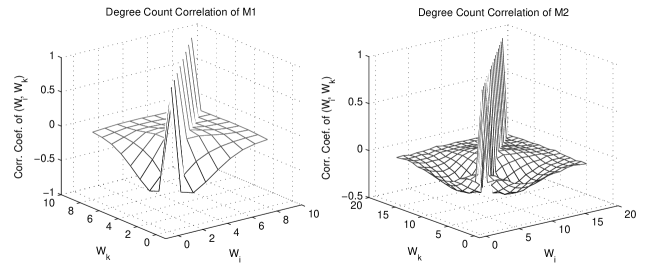
Figure 1 shows the correlations between the degree counts in the four models; except for Model M3 there is an appreciable correlation even far away from the diagonal.

Refer to caption
Refer to caption
Figure 1: Degree count correlation in Models M1 – M4.

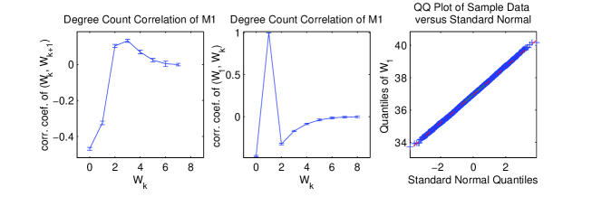
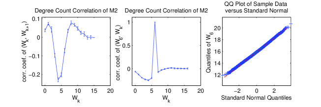
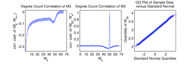
Figure 2 shows the degree count correlations, firstly between degree counts for kπ‘˜\displaystyle k and k+1π‘˜1\displaystyle k+1, and secondly for degree counts of an asymptotically normally distributed degree count and successive degree counts; the quantile-quantile plots are given for re-assurance. We observe a strong negative correlation for degree counts which are close by, but then close to zero correlation with counts of large degrees.

Refer to caption
Refer to caption
Refer to caption
Refer to caption
Figure 2: Degree count correlation and QQ plots in Models M1 – M4.

3.4 Simulations for Power-law Type Behavior

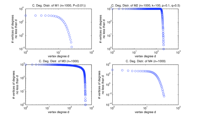
Using Models M1 – M4, but now with n=1,000𝑛1000\displaystyle n=1,000 vertices, we plot the number of vertices of degree no less than d𝑑\displaystyle d versus d𝑑\displaystyle d itself, on a log-log scale, Despite the networks being created using independent edges, the plots seem to display a sharp linear decline, which could easily be mis-interpreted as displaying a power-law behaviour.

Refer to caption
Figure 3: power law; log-log scale

These simulations confirm the pseudo-power-law phenomena, and therefore raise the issue that, without rigorous analysis, simulation-based claims of detecting power-law type behaviour, or scale-free behaviour, could be in fact unreliable and misleading. The vertex degree distribution may not be a suitable visual method for distinguishing different network models. In contrast, our distributional results help assess the joint distribution of vertex degrees under a fairly general null model.

4 Proofs

In this section, we provide proofs for the size-biased coupling construction 2.1, as well as for Theorem 4.3, Theorem 3.1, and Theorem 3.6. First we prove Lemma 2.2.

Proof 4.1

[Proof of Lemma 2.2] We first re-write f+​(𝐱i|𝐱d)superscript𝑓conditionalsubscript𝐱𝑖subscript𝐱𝑑\displaystyle f^{+}(\mathbf{x}_{i}\,|\,\mathbf{x}_{d}) as well as fβˆ’β€‹(𝐱i|𝐱d)superscript𝑓conditionalsubscript𝐱𝑖subscript𝐱𝑑\displaystyle f^{-}(\mathbf{x}_{i}\,|\,\mathbf{x}_{d}) by writing out the set N​(v)𝑁𝑣\displaystyle N(v) in terms of those vertices which remain fixed in the construction, and those which get added or removed, respectively. Here 𝐱isubscript𝐱𝑖\displaystyle\mathbf{x}_{i}, 𝐱dsubscript𝐱𝑑\displaystyle\mathbf{x}_{d}, 𝐲jsubscript𝐲𝑗\displaystyle\mathbf{y}_{j}, 𝐳(iβˆ’j)subscript𝐳𝑖𝑗\displaystyle\mathbf{z}_{(i-j)} and 𝐳(nβˆ’1βˆ’j+i)subscript𝐳𝑛1𝑗𝑖\displaystyle\mathbf{z}_{(n-1-j+i)} are all subsets of Vvsubscript𝑉𝑣\displaystyle V_{v}. Figure 4 illustrates the set relation in (4.1) and (4.1) respectively. We have

f+​(𝐱i|𝐱d)superscript𝑓conditionalsubscript𝐱𝑖subscript𝐱𝑑\displaystyle\displaystyle f^{+}(\mathbf{x}_{i}\,|\,\mathbf{x}_{d})
=\displaystyle\displaystyle= βˆ‘j=0iβˆ‘π²j:𝐲jβŠ‚π±iβˆ‘π³(iβˆ’j)βŠ‚Vvβˆ–π±d𝐳(iβˆ’j):1(dβˆ’jiβˆ’j)​ℙ​(N​(v)=𝐲jβˆͺ𝐳(iβˆ’j)|D​(v)=i),superscriptsubscript𝑗0𝑖subscript:subscript𝐲𝑗subscript𝐲𝑗subscript𝐱𝑖subscriptsuperscriptsubscript𝐳𝑖𝑗subscript𝑉𝑣subscript𝐱𝑑:subscript𝐳𝑖𝑗absent1FRACOP𝑑𝑗𝑖𝑗ℙ𝑁𝑣subscript𝐲𝑗conditionalsubscript𝐳𝑖𝑗𝐷𝑣𝑖\displaystyle\displaystyle\sum_{j=0}^{i}\,\sum_{\mathbf{y}_{j}:\mathbf{y}_{j}\subset\mathbf{x}_{i}}\sum_{\stackrel{{\scriptstyle\scriptsize\mbox{$\displaystyle\mathbf{z}_{(i-j)}:$}}}{{\scriptsize\mbox{$\displaystyle\mathbf{z}_{(i-j)}\subset V_{v}\setminus\mathbf{x}_{d}$}}}}\frac{1}{\genfrac{(}{)}{0.0pt}{}{d-j}{i-j}}\,\mathbb{P}(N(v)=\mathbf{y}_{j}\cup\mathbf{z}_{(i-j)}\,|\,D(v)=i),

and

fβˆ’β€‹(𝐱i|𝐱d)superscript𝑓conditionalsubscript𝐱𝑖subscript𝐱𝑑\displaystyle\displaystyle f^{-}(\mathbf{x}_{i}\,|\,\mathbf{x}_{d})
=\displaystyle\displaystyle= βˆ‘j=inβˆ’1βˆ‘π²j:𝐲jβŠƒπ±iβˆ‘π³(nβˆ’1βˆ’j+i)βŠƒVvβˆ–π±d𝐳(nβˆ’1βˆ’j+i):1(jβˆ’djβˆ’i)​ℙ​(N​(v)=𝐲j∩𝐳(nβˆ’1βˆ’j+i)|D​(v)=i).superscriptsubscript𝑗𝑖𝑛1subscript:subscript𝐲𝑗subscript𝐱𝑖subscript𝐲𝑗subscriptsuperscriptsubscript𝑉𝑣subscript𝐱𝑑subscript𝐳𝑛1𝑗𝑖:subscript𝐳𝑛1𝑗𝑖absent1FRACOP𝑗𝑑𝑗𝑖ℙ𝑁𝑣subscript𝐲𝑗conditionalsubscript𝐳𝑛1𝑗𝑖𝐷𝑣𝑖\displaystyle\displaystyle\sum_{j=i}^{n-1}\sum_{\mathbf{y}_{j}:\mathbf{y}_{j}\supset\mathbf{x}_{i}}\sum_{\stackrel{{\scriptstyle\scriptsize\mbox{$\displaystyle\mathbf{z}_{(n-1-j+i)}:$}}}{{\scriptsize\mbox{$\displaystyle\mathbf{z}_{(n-1-j+i)}\supset V_{v}\setminus\mathbf{x}_{d}$}}}}\frac{1}{\genfrac{(}{)}{0.0pt}{}{j-d}{j-i}}\mathbb{P}(N(v)=\mathbf{y}_{j}\cap\mathbf{z}_{(n-1-j+i)}|D(v)=i).
Refer to caption
Refer to caption
Figure 4: The set diagram for the expression (4.1) (left) and (4.1) (right), respectively.

See Lemma 4.3.2 in Lin [11] for more details.

Now, from (4.1), since, for any 𝐱dsubscript𝐱𝑑\displaystyle\mathbf{x}_{d} and 𝐲jsubscript𝐲𝑗\displaystyle\mathbf{y}_{j}, there are (dβˆ’jiβˆ’j)𝐹𝑅𝐴𝐢𝑂𝑃𝑑𝑗𝑖𝑗\displaystyle\genfrac{(}{)}{0.0pt}{}{d-j}{i-j} choices of 𝐱isubscript𝐱𝑖\displaystyle\mathbf{x}_{i}, we have

βˆ‘π±i:𝐱iβŠ‚π±df+​(𝐱i|𝐱d)subscript:subscript𝐱𝑖subscript𝐱𝑖subscript𝐱𝑑superscript𝑓conditionalsubscript𝐱𝑖subscript𝐱𝑑\displaystyle\displaystyle\sum_{\mathbf{x}_{i}:\mathbf{x}_{i}\subset\mathbf{x}_{d}}f^{+}(\mathbf{x}_{i}\,|\,\mathbf{x}_{d})
=\displaystyle\displaystyle= 1ℙ​(D​(v)=i)β€‹βˆ‘j=0iβˆ‘π²j:𝐲jβŠ‚π±dβˆ‘π³(iβˆ’j)βŠ‚Vvβˆ–π±d𝐳(iβˆ’j):ℙ​(N​(v)=𝐲jβˆͺ𝐳(iβˆ’j)).1ℙ𝐷𝑣𝑖superscriptsubscript𝑗0𝑖subscript:subscript𝐲𝑗subscript𝐲𝑗subscript𝐱𝑑subscriptsuperscriptsubscript𝐳𝑖𝑗subscript𝑉𝑣subscript𝐱𝑑:subscript𝐳𝑖𝑗absentℙ𝑁𝑣subscript𝐲𝑗subscript𝐳𝑖𝑗\displaystyle\displaystyle\frac{1}{\mathbb{P}(D(v)=i)}\sum_{j=0}^{i}\sum_{\mathbf{y}_{j}:\mathbf{y}_{j}\subset\mathbf{x}_{d}}\sum_{\stackrel{{\scriptstyle\scriptsize\mbox{$\displaystyle\mathbf{z}_{(i-j)}:$}}}{{\scriptsize\mbox{$\displaystyle\mathbf{z}_{(i-j)}\subset V_{v}\setminus\mathbf{x}_{d}$}}}}\mathbb{P}(N(v)=\mathbf{y}_{j}\cup\mathbf{z}_{(i-j)}).

Let 𝐗i={𝐱i:𝐱iβŠ‚Vv}subscript𝐗𝑖conditional-setsubscript𝐱𝑖subscript𝐱𝑖subscript𝑉𝑣\displaystyle\mathbf{X}_{i}=\{\mathbf{x}_{i}:\mathbf{x}_{i}\subset V_{v}\}. Note that π›šiβˆˆπ—isubscriptπ›šπ‘–subscript𝐗𝑖\displaystyle\bm{\omega}_{i}\in\mathbf{X}_{i} if and only if π›šisubscriptπ›šπ‘–\displaystyle\bm{\omega}_{i} can be uniquely decomposed as π›ši=𝐲jβˆͺ𝐳(iβˆ’j)subscriptπ›šπ‘–subscript𝐲𝑗subscript𝐳𝑖𝑗\displaystyle\bm{\omega}_{i}=\mathbf{y}_{j}\cup\mathbf{z}_{(i-j)} such that 𝐲jβŠ‚π±dsubscript𝐲𝑗subscript𝐱𝑑\displaystyle\mathbf{y}_{j}\subset\mathbf{x}_{d} and 𝐳(iβˆ’j)βŠ‚Vvβˆ–π±dsubscript𝐳𝑖𝑗subscript𝑉𝑣subscript𝐱𝑑\displaystyle\mathbf{z}_{(i-j)}\subset V_{v}\setminus\mathbf{x}_{d}. Thus,

βˆ‘π±i:𝐱iβŠ‚π±df+​(𝐱i|𝐱d)=1ℙ​(D​(v)=i)β€‹βˆ‘πŽiβˆˆπ—iℙ​(N​(v)=𝝎i)=1,subscript:subscript𝐱𝑖subscript𝐱𝑖subscript𝐱𝑑superscript𝑓conditionalsubscript𝐱𝑖subscript𝐱𝑑1ℙ𝐷𝑣𝑖subscriptsubscriptπŽπ‘–subscript𝐗𝑖ℙ𝑁𝑣subscriptπŽπ‘–1\displaystyle\displaystyle\sum_{\mathbf{x}_{i}:\mathbf{x}_{i}\subset\mathbf{x}_{d}}f^{+}(\mathbf{x}_{i}\,|\,\mathbf{x}_{d})=\frac{1}{\mathbb{P}(D(v)=i)}\sum_{\bm{\omega}_{i}\in\mathbf{X}_{i}}\mathbb{P}(N(v)=\bm{\omega}_{i})=1,

as required. Similarly, from (4.1) we find that

βˆ‘π±i:𝐱iβŠƒπ±dfβˆ’β€‹(𝐱i|𝐱d)subscript:subscript𝐱𝑖subscript𝐱𝑑subscript𝐱𝑖superscript𝑓conditionalsubscript𝐱𝑖subscript𝐱𝑑\displaystyle\displaystyle\sum_{\mathbf{x}_{i}:\mathbf{x}_{i}\supset\mathbf{x}_{d}}f^{-}(\mathbf{x}_{i}\,|\,\mathbf{x}_{d})
=\displaystyle\displaystyle= 1ℙ​(D​(v)=i)β€‹βˆ‘j=inβˆ’1βˆ‘π²j:𝐲jβŠƒπ±dβˆ‘π³(nβˆ’1βˆ’j+i)βŠƒVvβˆ–π±d𝐳(nβˆ’1βˆ’j+i):ℙ​(N​(v)=𝐲j∩𝐳(nβˆ’1βˆ’j+i)).1ℙ𝐷𝑣𝑖superscriptsubscript𝑗𝑖𝑛1subscript:subscript𝐲𝑗subscript𝐱𝑑subscript𝐲𝑗subscriptsuperscriptsubscript𝑉𝑣subscript𝐱𝑑subscript𝐳𝑛1𝑗𝑖:subscript𝐳𝑛1𝑗𝑖absentℙ𝑁𝑣subscript𝐲𝑗subscript𝐳𝑛1𝑗𝑖\displaystyle\displaystyle\frac{1}{\mathbb{P}(D(v)=i)}\sum_{j=i}^{n-1}\sum_{\mathbf{y}_{j}:\mathbf{y}_{j}\supset\mathbf{x}_{d}}\sum_{\stackrel{{\scriptstyle\scriptsize\mbox{$\displaystyle\mathbf{z}_{(n-1-j+i)}:$}}}{{\scriptsize\mbox{$\displaystyle\mathbf{z}_{(n-1-j+i)}\supset V_{v}\setminus\mathbf{x}_{d}$}}}}\mathbb{P}(N(v)=\mathbf{y}_{j}\cap\mathbf{z}_{(n-1-j+i)}).

Note that, π›šiβˆˆπ—isubscriptπ›šπ‘–subscript𝐗𝑖\displaystyle\bm{\omega}_{i}\in\mathbf{X}_{i} if and only if π›šisubscriptπ›šπ‘–\displaystyle\bm{\omega}_{i} can be uniquely written as π›ši=𝐲j∩𝐳(nβˆ’1βˆ’j+i)subscriptπ›šπ‘–subscript𝐲𝑗subscript𝐳𝑛1𝑗𝑖\displaystyle\bm{\omega}_{i}=\mathbf{y}_{j}\cap\mathbf{z}_{(n-1-j+i)} such that 𝐲jβŠƒπ±dsubscript𝐱𝑑subscript𝐲𝑗\displaystyle\mathbf{y}_{j}\supset\mathbf{x}_{d} and 𝐳(nβˆ’1βˆ’j+i)βŠƒVvβˆ–π±dsubscript𝑉𝑣subscript𝐱𝑑subscript𝐳𝑛1𝑗𝑖\displaystyle\mathbf{z}_{(n-1-j+i)}\supset V_{v}\setminus\mathbf{x}_{d}. Thus,

βˆ‘π±i:𝐱iβŠƒπ±dfβˆ’β€‹(𝐱i|𝐱d)=1ℙ​(D​(v)=i)β€‹βˆ‘πŽiβˆˆπ—iℙ​(N​(v)=𝝎i)=1,subscript:subscript𝐱𝑖subscript𝐱𝑑subscript𝐱𝑖superscript𝑓conditionalsubscript𝐱𝑖subscript𝐱𝑑1ℙ𝐷𝑣𝑖subscriptsubscriptπŽπ‘–subscript𝐗𝑖ℙ𝑁𝑣subscriptπŽπ‘–1\displaystyle\displaystyle\sum_{\mathbf{x}_{i}:\mathbf{x}_{i}\supset\mathbf{x}_{d}}f^{-}(\mathbf{x}_{i}\,|\,\mathbf{x}_{d})=\frac{1}{\mathbb{P}(D(v)=i)}\sum_{\bm{\omega}_{i}\in\mathbf{X}_{i}}\mathbb{P}(N(v)=\bm{\omega}_{i})=1,

as required.

Proof 4.2 (Proof of Construction 2.1)

The goal of this proof is to show that, for Ξ²=(v,i)βˆˆΞ“π›½π‘£π‘–Ξ“\displaystyle\beta=(v,i)\in\Gamma,

ℒ​(𝐗β)=ℒ​(𝐗|XΞ²=1),β„’superscript𝐗𝛽ℒconditional𝐗subscript𝑋𝛽1\displaystyle\displaystyle\mathcal{L}(\mathbf{X}^{\beta})=\mathcal{L}(\mathbf{X}\,|\,X_{\beta}=1), (4.3)

where 𝐗={X(v,i):(v,i)βˆˆΞ“}𝐗conditional-setsubscript𝑋𝑣𝑖𝑣𝑖Γ\displaystyle\mathbf{X}=\{X_{(v,i)}:(v,i)\in\Gamma\} and 𝐗β={X(v,i)Ξ²:(v,i)βˆˆΞ“}superscript𝐗𝛽conditional-setsuperscriptsubscript𝑋𝑣𝑖𝛽𝑣𝑖Γ\displaystyle\mathbf{X}^{\beta}=\{X_{(v,i)}^{\beta}:(v,i)\in\Gamma\}. Indeed we shall show that the distribution of the constructed model 𝒒β​(n,{pi​j})superscript𝒒𝛽𝑛subscript𝑝𝑖𝑗\displaystyle\mathscr{G}^{\beta}(n,\{p_{ij}\}) is the same as the conditional distribution of the original model 𝒒​(n,{pi​j})𝒒𝑛subscript𝑝𝑖𝑗\displaystyle\mathscr{G}(n,\{p_{ij}\}) given XΞ²=1subscript𝑋𝛽1\displaystyle X_{\beta}=1, that is, with 𝐗e​d​g​e={X{a,b}:{a,b}∈E}subscript𝐗𝑒𝑑𝑔𝑒conditional-setsubscriptπ‘‹π‘Žπ‘π‘Žπ‘πΈ\displaystyle\mathbf{X}_{edge}=\{X_{\{a,b\}}:\{a,b\}\in E\} and 𝐗e​d​g​eΞ²={X{a,b}Ξ²:{a,b}∈E}superscriptsubscript𝐗𝑒𝑑𝑔𝑒𝛽conditional-setsuperscriptsubscriptπ‘‹π‘Žπ‘π›½π‘Žπ‘πΈ\displaystyle\mathbf{X}_{edge}^{\beta}=\{X_{\{a,b\}}^{\beta}:\{a,b\}\in E\}, we meed to show that for all 𝐰:=(wa,b,{a,b}∈E)∈{0,1}|E|assign𝐰subscriptπ‘€π‘Žπ‘π‘Žπ‘πΈsuperscript01𝐸\displaystyle\mathbf{w}:=(w_{a,b},\{a,b\}\in E)\in\{0,1\}^{|E|},

ℙ​(𝐗e​d​g​e(v,i)=𝐰)=ℙ​(𝐗e​d​g​e=𝐰|X(v,i)=1).β„™subscriptsuperscript𝐗𝑣𝑖𝑒𝑑𝑔𝑒𝐰ℙsubscript𝐗𝑒𝑑𝑔𝑒conditional𝐰subscript𝑋𝑣𝑖1\displaystyle\displaystyle\mathbb{P}(\mathbf{X}^{(v,i)}_{edge}=\mathbf{w})=\mathbb{P}(\mathbf{X}_{edge}=\mathbf{w}\,|\,X_{(v,i)}=1). (4.4)

The desired equation (4.3) then follows because 𝐗𝐗\displaystyle\mathbf{X} is a function of 𝐗e​d​g​esubscript𝐗𝑒𝑑𝑔𝑒\displaystyle\mathbf{X}_{edge}.

By definition of X(v,i)subscript𝑋𝑣𝑖\displaystyle X_{(v,i)}, the right-hand side of (4.4) is zero when Ξ£x∈Vv​wv,xβ‰ isubscriptΞ£π‘₯subscript𝑉𝑣subscript𝑀𝑣π‘₯𝑖\displaystyle\Sigma_{x\in V_{v}}w_{v,x}\neq i, and by construction in that case the left-hand side of (4.4) is zero also. Assume that Ξ£x∈Vv​wv,x=isubscriptΞ£π‘₯subscript𝑉𝑣subscript𝑀𝑣π‘₯𝑖\displaystyle\Sigma_{x\in V_{v}}w_{v,x}=i, then the right-hand sice of (4.4) equals

ℙ​(𝐗e​d​g​e=𝐰|X(v,i)=1)=ℙ​(𝐗e​d​g​e=𝐰|D​(v)=i)β„™subscript𝐗𝑒𝑑𝑔𝑒conditional𝐰subscript𝑋𝑣𝑖1β„™subscript𝐗𝑒𝑑𝑔𝑒conditional𝐰𝐷𝑣𝑖\displaystyle\displaystyle\mathbb{P}(\mathbf{X}_{edge}=\mathbf{w}|X_{(v,i)}=1)=\mathbb{P}(\mathbf{X}_{edge}=\mathbf{w}\,|\,D(v)=i) (4.5)
=\displaystyle\displaystyle= β„™(X{a,b}=wa,bβˆ€aβ‰ v,bβ‰ v;N(v)={x∈Vv:wv,x=1}|D(v)=i)\displaystyle\displaystyle\mathbb{P}(X_{\{a,b\}}=w_{a,b}\forall a\neq v,\;b\neq v;\;N(v)=\{x\in V_{v}:w_{v,x}=1\}\,|\,D(v)=i)
=\displaystyle\displaystyle= β„™(X{a,b}=wa,bβˆ€aβ‰ v,bβ‰ v)β„™(N(v)=𝐱i|D(v)=i),\displaystyle\displaystyle\mathbb{P}(X_{\{a,b\}}=w_{a,b}\;\forall\;a\neq v,\;b\neq v)\mathbb{P}(N(v)=\mathbf{x}_{i}\,|\,D(v)=i),

where the last equality follows from the independence of the edges, as the condition D​(v)=i𝐷𝑣𝑖\displaystyle D(v)=i only affects (X{v,x},x∈Vv)subscript𝑋𝑣π‘₯π‘₯subscript𝑉𝑣\displaystyle(X_{\{v,x\}},x\in V_{v}), but not edges which do not contain v𝑣\displaystyle v. On the other hand, the left hand side of (4.4) equals

β„™(X{a,b}=wa,bfor allaβ‰ v,bβ‰ v;X{v,x}(v,i)=wv,xforx∈Vv)\displaystyle\displaystyle\mathbb{P}(X_{\{a,b\}}=w_{a,b}\;\mbox{for all}\;a\neq v,\;b\neq v;\;X_{\{v,x\}}^{(v,i)}=w_{v,x}\;\mbox{for}\;x\in V_{v}) (4.6)
=\displaystyle\displaystyle= β„™(X{a,b}=wa,bfor allaβ‰ v,bβ‰ v)β„™(X{v,x}(v,i)=wv,xforx∈Vv),\displaystyle\displaystyle\mathbb{P}(X_{\{a,b\}}=w_{a,b}\;\mbox{for all}\;a\neq v,\;b\neq v)\mathbb{P}(X_{\{v,x\}}^{(v,i)}=w_{v,x}\;\mbox{for}\;x\in V_{v}),\qquad

as the construction of 𝐗e​d​g​e(v,i)subscriptsuperscript𝐗𝑣𝑖𝑒𝑑𝑔𝑒\displaystyle\mathbf{X}^{(v,i)}_{edge} from 𝐗e​d​g​esubscript𝐗𝑒𝑑𝑔𝑒\displaystyle\mathbf{X}_{edge} affects only the edges with v𝑣\displaystyle v as one of its end points, and the edges are independent. Note that, in (4.6),

ℙ​(X{v,x}(v,i)=wv,xβ€‹βˆ€x∈Vv)=ℙ​(N(v,i)​(v)=𝐱i).β„™superscriptsubscript𝑋𝑣π‘₯𝑣𝑖subscript𝑀𝑣π‘₯for-allπ‘₯subscript𝑉𝑣ℙsuperscript𝑁𝑣𝑖𝑣subscript𝐱𝑖\displaystyle\displaystyle\mathbb{P}(X_{\{v,x\}}^{(v,i)}=w_{v,x}\forall x\in V_{v})=\mathbb{P}(N^{(v,i)}(v)=\mathbf{x}_{i}).

Hence to conclude that (4.6) equals (4.5), it remains to show that

ℙ​(N(v,i)​(v)=𝐱i)=ℙ​(N​(v)=𝐱i|D​(v)=i).β„™superscript𝑁𝑣𝑖𝑣subscript𝐱𝑖ℙ𝑁𝑣conditionalsubscript𝐱𝑖𝐷𝑣𝑖\displaystyle\displaystyle\mathbb{P}(N^{(v,i)}(v)=\mathbf{x}_{i})=\mathbb{P}(N(v)=\mathbf{x}_{i}\,|\,D(v)=i). (4.7)

Indeed,

ℙ​(N(v,i)​(v)=𝐱i)β„™superscript𝑁𝑣𝑖𝑣subscript𝐱𝑖\displaystyle\displaystyle\mathbb{P}(N^{(v,i)}(v)=\mathbf{x}_{i})
=\displaystyle\displaystyle= qv,i​ℙ​(N​(v)=𝐱i|D​(v)=i)subscriptπ‘žπ‘£π‘–β„™π‘π‘£conditionalsubscript𝐱𝑖𝐷𝑣𝑖\displaystyle\displaystyle q_{v,i}\mathbb{P}(N(v)=\mathbf{x}_{i}\,|\,D(v)=i)
+βˆ‘d:d>iqv,dβ€‹βˆ‘π±d:𝐱dβŠƒπ±iℙ​(N​(v)=𝐱d|D​(v)=d)​ℙ​(N(v,i)​(v)=𝐱i|N​(v)=𝐱d)subscript:𝑑𝑑𝑖subscriptπ‘žπ‘£π‘‘subscript:subscript𝐱𝑑subscript𝐱𝑖subscript𝐱𝑑ℙ𝑁𝑣conditionalsubscript𝐱𝑑𝐷𝑣𝑑ℙsuperscript𝑁𝑣𝑖𝑣conditionalsubscript𝐱𝑖𝑁𝑣subscript𝐱𝑑\displaystyle\displaystyle+\sum_{d:d>i}q_{v,d}\sum_{\mathbf{x}_{d}:\mathbf{x}_{d}\supset\mathbf{x}_{i}}\mathbb{P}(N(v)=\mathbf{x}_{d}|D(v)=d)\mathbb{P}(N^{(v,i)}(v)=\mathbf{x}_{i}|N(v)=\mathbf{x}_{d})
+βˆ‘d:d<iqv,dβ€‹βˆ‘π±d:𝐱dβŠ‚π±iℙ​(N​(v)=𝐱d|D​(v)=d)​ℙ​(N(v,i)​(v)=𝐱i|N​(v)=𝐱d),subscript:𝑑𝑑𝑖subscriptπ‘žπ‘£π‘‘subscript:subscript𝐱𝑑subscript𝐱𝑑subscript𝐱𝑖ℙ𝑁𝑣conditionalsubscript𝐱𝑑𝐷𝑣𝑑ℙsuperscript𝑁𝑣𝑖𝑣conditionalsubscript𝐱𝑖𝑁𝑣subscript𝐱𝑑\displaystyle\displaystyle+\sum_{d:d<i}q_{v,d}\sum_{\mathbf{x}_{d}:\mathbf{x}_{d}\subset\mathbf{x}_{i}}\mathbb{P}(N(v)=\mathbf{x}_{d}|D(v)=d)\mathbb{P}(N^{(v,i)}(v)=\mathbf{x}_{i}|N(v)=\mathbf{x}_{d}),

where the three terms corresponding to the coupling construction (2.1). Now, we calculate the sums over 𝐱d:𝐱dβŠƒπ±i:subscript𝐱𝑑subscript𝐱𝑖subscript𝐱𝑑\displaystyle\mathbf{x}_{d}:\mathbf{x}_{d}\supset\mathbf{x}_{i} and over 𝐱d:𝐱dβŠ‚π±i:subscript𝐱𝑑subscript𝐱𝑑subscript𝐱𝑖\displaystyle\mathbf{x}_{d}:\mathbf{x}_{d}\subset\mathbf{x}_{i} separately. In fact, for the first case d>i𝑑𝑖\displaystyle d>i and 𝐱dβŠƒπ±isubscript𝐱𝑖subscript𝐱𝑑\displaystyle\mathbf{x}_{d}\supset\mathbf{x}_{i}, it follows from (2.1) and (4.1) that

βˆ‘π±d:𝐱dβŠƒπ±iℙ​(N​(v)=𝐱d|D​(v)=d)​ℙ​(N(v,i)​(v)=𝐱i|N​(v)=𝐱d)subscript:subscript𝐱𝑑subscript𝐱𝑖subscript𝐱𝑑ℙ𝑁𝑣conditionalsubscript𝐱𝑑𝐷𝑣𝑑ℙsuperscript𝑁𝑣𝑖𝑣conditionalsubscript𝐱𝑖𝑁𝑣subscript𝐱𝑑\displaystyle\displaystyle\sum_{\mathbf{x}_{d}:\mathbf{x}_{d}\supset\mathbf{x}_{i}}\mathbb{P}(N(v)=\mathbf{x}_{d}\,|\,D(v)=d)\mathbb{P}(N^{(v,i)}(v)=\mathbf{x}_{i}\,|\,N(v)=\mathbf{x}_{d})
=\displaystyle\displaystyle= βˆ‘j=0iβˆ‘π±dβŠƒπ±i𝐱d:βˆ‘π²jβŠ‚π±i𝐲j:βˆ‘π³(iβˆ’j)βŠ‚Vvβˆ–π±d𝐳(iβˆ’j):1(dβˆ’jiβˆ’j)superscriptsubscript𝑗0𝑖subscriptsuperscriptsubscript𝐱𝑖subscript𝐱𝑑:subscript𝐱𝑑absentsubscriptsuperscriptsubscript𝐲𝑗subscript𝐱𝑖:subscript𝐲𝑗absentsubscriptsuperscriptsubscript𝐳𝑖𝑗subscript𝑉𝑣subscript𝐱𝑑:subscript𝐳𝑖𝑗absent1FRACOP𝑑𝑗𝑖𝑗\displaystyle\displaystyle\sum_{j=0}^{i}\;\sum_{\stackrel{{\scriptstyle\scriptsize\mbox{$\displaystyle\mathbf{x}_{d}:$}}}{{\scriptsize\mbox{$\displaystyle\mathbf{x}_{d}\supset\mathbf{x}_{i}$}}}}\;\sum_{\stackrel{{\scriptstyle\scriptsize\mbox{$\displaystyle\mathbf{y}_{j}:$}}}{{\scriptsize\mbox{$\displaystyle\mathbf{y}_{j}\subset\mathbf{x}_{i}$}}}}\;\sum_{\stackrel{{\scriptstyle\scriptsize\mbox{$\displaystyle\mathbf{z}_{(i-j)}:$}}}{{\scriptsize\mbox{$\displaystyle\mathbf{z}_{(i-j)}\subset V_{v}\setminus\mathbf{x}_{d}$}}}}\frac{1}{\genfrac{(}{)}{0.0pt}{}{d-j}{i-j}}
×ℙ​(N​(v)=𝐱d)​ℙ​(N​(v)=𝐲jβˆͺ𝐳(iβˆ’j))ℙ​(D​(v)=d)​ℙ​(D​(v)=i),absentℙ𝑁𝑣subscript𝐱𝑑ℙ𝑁𝑣subscript𝐲𝑗subscript𝐳𝑖𝑗ℙ𝐷𝑣𝑑ℙ𝐷𝑣𝑖\displaystyle\displaystyle\times\frac{\mathbb{P}(N(v)=\mathbf{x}_{d})\mathbb{P}(N(v)=\mathbf{y}_{j}\cup\mathbf{z}_{(i-j)})}{\mathbb{P}(D(v)=d)\mathbb{P}(D(v)=i)},

where

ℙ​(N​(v)=𝐱d)ℙ𝑁𝑣subscript𝐱𝑑\displaystyle\displaystyle\mathbb{P}(N(v)=\mathbf{x}_{d}) =\displaystyle\displaystyle= [(∏x∈𝐱dpv​x)​(∏x∈Vvβˆ–π±d(1βˆ’pv​x))].delimited-[]subscriptproductπ‘₯subscript𝐱𝑑subscript𝑝𝑣π‘₯subscriptproductπ‘₯subscript𝑉𝑣subscript𝐱𝑑1subscript𝑝𝑣π‘₯\displaystyle\displaystyle\bigg{[}\Big{(}\prod_{x\in\mathbf{x}_{d}}p_{vx}\Big{)}\Big{(}\prod_{x\in V_{v}\setminus\mathbf{x}_{d}}(1-p_{vx})\Big{)}\bigg{]}.

Since 𝐲jβŠ‚π±iβŠ‚π±dsubscript𝐲𝑗subscript𝐱𝑖subscript𝐱𝑑\displaystyle\mathbf{y}_{j}\subset\mathbf{x}_{i}\subset\mathbf{x}_{d} and 𝐳(iβˆ’j)βŠ‚Vvβˆ–π±dsubscript𝐳𝑖𝑗subscript𝑉𝑣subscript𝐱𝑑\displaystyle\mathbf{z}_{(i-j)}\subset V_{v}\setminus\mathbf{x}_{d}, we have Vvβˆ–(𝐲jβˆͺ𝐳(iβˆ’j))βŠƒπ±dβˆ–π±isubscript𝐱𝑑subscript𝐱𝑖subscript𝑉𝑣subscript𝐲𝑗subscript𝐳𝑖𝑗\displaystyle V_{v}\setminus(\mathbf{y}_{j}\cup\mathbf{z}_{(i-j)})\supset\mathbf{x}_{d}\setminus\mathbf{x}_{i} (see Figure 4 for reference). Therefore,

ℙ​(N​(v)=𝐱d)​ℙ​(N​(v)=𝐲jβˆͺ𝐳(iβˆ’j))ℙ𝑁𝑣subscript𝐱𝑑ℙ𝑁𝑣subscript𝐲𝑗subscript𝐳𝑖𝑗\displaystyle\displaystyle{\mathbb{P}(N(v)=\mathbf{x}_{d})\mathbb{P}(N(v)=\mathbf{y}_{j}\cup\mathbf{z}_{(i-j)})}
=\displaystyle\displaystyle= [(∏x∈𝐱ipv​x)​(∏x∈Vvβˆ–π±d(1βˆ’pv​x))​(∏x∈𝐱dβˆ–π±i(1βˆ’pv​x))]delimited-[]subscriptproductπ‘₯subscript𝐱𝑖subscript𝑝𝑣π‘₯subscriptproductπ‘₯subscript𝑉𝑣subscript𝐱𝑑1subscript𝑝𝑣π‘₯subscriptproductπ‘₯subscript𝐱𝑑subscript𝐱𝑖1subscript𝑝𝑣π‘₯\displaystyle\displaystyle\bigg{[}\Big{(}\prod_{x\in\mathbf{x}_{i}}p_{vx}\Big{)}\Big{(}\prod_{x\in V_{v}\setminus\mathbf{x}_{d}}(1-p_{vx})\Big{)}\Big{(}\prod_{x\in\mathbf{x}_{d}\setminus\mathbf{x}_{i}}(1-p_{vx})\Big{)}\bigg{]}
β‹…[(∏x∈𝐱dβˆ–π±ipv​x)​(∏x∈𝐲jβˆͺ𝐳(iβˆ’j)pv​x)​(∏x∈Vvβˆ–[𝐲jβˆͺ𝐳(iβˆ’j)βˆͺ(𝐱dβˆ–π±i)](1βˆ’pv​x))]β‹…absentdelimited-[]subscriptproductπ‘₯subscript𝐱𝑑subscript𝐱𝑖subscript𝑝𝑣π‘₯subscriptproductπ‘₯subscript𝐲𝑗subscript𝐳𝑖𝑗subscript𝑝𝑣π‘₯subscriptproductπ‘₯subscript𝑉𝑣delimited-[]subscript𝐲𝑗subscript𝐳𝑖𝑗subscript𝐱𝑑subscript𝐱𝑖1subscript𝑝𝑣π‘₯\displaystyle\displaystyle\cdot\bigg{[}\Big{(}\prod_{x\in\mathbf{x}_{d}\setminus\mathbf{x}_{i}}p_{vx}\Big{)}\Big{(}\prod_{x\in\mathbf{y}_{j}\cup\mathbf{z}_{(i-j)}}p_{vx}\Big{)}\Big{(}\prod_{x\in V_{v}\setminus[\mathbf{y}_{j}\cup\mathbf{z}_{(i-j)}\cup(\mathbf{x}_{d}\setminus\mathbf{x}_{i})]}(1-p_{vx})\Big{)}\bigg{]}
=\displaystyle\displaystyle= ℙ​(N​(v)=𝐱i)​ℙ​(N​(v)=𝐲jβˆͺ𝐳(iβˆ’j)βˆͺ(𝐱dβˆ–π±i)).ℙ𝑁𝑣subscript𝐱𝑖ℙ𝑁𝑣subscript𝐲𝑗subscript𝐳𝑖𝑗subscript𝐱𝑑subscript𝐱𝑖\displaystyle\displaystyle\mathbb{P}(N(v)=\mathbf{x}_{i})\mathbb{P}\big{(}N(v)=\mathbf{y}_{j}\cup\mathbf{z}_{(i-j)}\cup(\mathbf{x}_{d}\setminus\mathbf{x}_{i})\big{)}.

Hence, from (4.2), we have for d>i𝑑𝑖\displaystyle d>i that

βˆ‘π±d:𝐱dβŠƒπ±iℙ​(N​(v)=𝐱d|D​(v)=d)​ℙ​(N(v,i)​(v)=𝐱i|N​(v)=𝐱d)subscript:subscript𝐱𝑑subscript𝐱𝑖subscript𝐱𝑑ℙ𝑁𝑣conditionalsubscript𝐱𝑑𝐷𝑣𝑑ℙsuperscript𝑁𝑣𝑖𝑣conditionalsubscript𝐱𝑖𝑁𝑣subscript𝐱𝑑\displaystyle\displaystyle{\sum_{\mathbf{x}_{d}:\mathbf{x}_{d}\supset\mathbf{x}_{i}}\mathbb{P}(N(v)=\mathbf{x}_{d}\,|\,D(v)=d)\mathbb{P}(N^{(v,i)}(v)=\mathbf{x}_{i}\,|\,N(v)=\mathbf{x}_{d})}
=ℙ​(N​(v)=𝐱i)ℙ​(D​(v)=i)β‹…1ℙ​(D​(v)=d)β€‹βˆ‘j=0i1(dβˆ’jiβˆ’j)absent⋅ℙ𝑁𝑣subscript𝐱𝑖ℙ𝐷𝑣𝑖1ℙ𝐷𝑣𝑑superscriptsubscript𝑗0𝑖1FRACOP𝑑𝑗𝑖𝑗\displaystyle\displaystyle=\frac{\mathbb{P}(N(v)=\mathbf{x}_{i})}{\mathbb{P}(D(v)=i)}\cdot\frac{1}{\mathbb{P}(D(v)=d)}\sum_{j=0}^{i}\frac{1}{\genfrac{(}{)}{0.0pt}{}{d-j}{i-j}}\; (4.10)
βˆ‘π±dβŠƒπ±i𝐱d:βˆ‘π²jβŠ‚π±i𝐲j:βˆ‘π³(iβˆ’j)βŠ‚Vvβˆ–π±d𝐳(iβˆ’j):ℙ​(N​(v)=𝐲jβˆͺ𝐳(iβˆ’j)βˆͺ(𝐱dβˆ–π±i)).subscriptsuperscriptsubscript𝐱𝑖subscript𝐱𝑑:subscript𝐱𝑑absentsubscriptsuperscriptsubscript𝐲𝑗subscript𝐱𝑖:subscript𝐲𝑗absentsubscriptsuperscriptsubscript𝐳𝑖𝑗subscript𝑉𝑣subscript𝐱𝑑:subscript𝐳𝑖𝑗absentℙ𝑁𝑣subscript𝐲𝑗subscript𝐳𝑖𝑗subscript𝐱𝑑subscript𝐱𝑖\displaystyle\displaystyle\sum_{\stackrel{{\scriptstyle\scriptsize\mbox{$\displaystyle\mathbf{x}_{d}:$}}}{{\scriptsize\mbox{$\displaystyle\mathbf{x}_{d}\supset\mathbf{x}_{i}$}}}}\;\sum_{\stackrel{{\scriptstyle\scriptsize\mbox{$\displaystyle\mathbf{y}_{j}:$}}}{{\scriptsize\mbox{$\displaystyle\mathbf{y}_{j}\subset\mathbf{x}_{i}$}}}}\;\sum_{\stackrel{{\scriptstyle\scriptsize\mbox{$\displaystyle\mathbf{z}_{(i-j)}:$}}}{{\scriptsize\mbox{$\displaystyle\mathbf{z}_{(i-j)}\subset V_{v}\setminus\mathbf{x}_{d}$}}}}\,\mathbb{P}\big{(}N(v)=\mathbf{y}_{j}\cup\mathbf{z}_{(i-j)}\cup(\mathbf{x}_{d}\setminus\mathbf{x}_{i})\big{)}.

Since 𝐲jβˆͺ𝐳(iβˆ’j)subscript𝐲𝑗subscript𝐳𝑖𝑗\displaystyle\mathbf{y}_{j}\cup\mathbf{z}_{(i-j)} is an i𝑖\displaystyle i-set (i.e. a set with i𝑖\displaystyle i elements), (𝐱dβˆ–π±i)subscript𝐱𝑑subscript𝐱𝑖\displaystyle(\mathbf{x}_{d}\setminus\mathbf{x}_{i}) is a (dβˆ’i)𝑑𝑖\displaystyle(d-i)-set, and (𝐲jβˆͺ𝐳(iβˆ’j))∩(𝐱dβˆ–π±i)=βˆ…subscript𝐲𝑗subscript𝐳𝑖𝑗subscript𝐱𝑑subscript𝐱𝑖\displaystyle(\mathbf{y}_{j}\cup\mathbf{z}_{(i-j)})\cap(\mathbf{x}_{d}\setminus\mathbf{x}_{i})=\emptyset, we have that 𝐲jβˆͺ𝐳(iβˆ’j)βˆͺ(𝐱dβˆ–π±i)subscript𝐲𝑗subscript𝐳𝑖𝑗subscript𝐱𝑑subscript𝐱𝑖\displaystyle\mathbf{y}_{j}\cup\mathbf{z}_{(i-j)}\cup(\mathbf{x}_{d}\setminus\mathbf{x}_{i}) is a d𝑑\displaystyle d-set in 𝐗dsubscript𝐗𝑑\displaystyle\mathbf{X}_{d}. Conversely, for any d𝑑\displaystyle d-set π›šdβˆˆπ—dsubscriptπ›šπ‘‘subscript𝐗𝑑\displaystyle\bm{\omega}_{d}\in\mathbf{X}_{d}, since 𝐱isubscript𝐱𝑖\displaystyle\mathbf{x}_{i} is fixed, we can decompose π›šdsubscriptπ›šπ‘‘\displaystyle\bm{\omega}_{d} as

𝝎d=𝐲jβˆͺ𝐳(iβˆ’j)βˆͺ(𝐱dβˆ–π±i),subscriptπŽπ‘‘subscript𝐲𝑗subscript𝐳𝑖𝑗subscript𝐱𝑑subscript𝐱𝑖\displaystyle\displaystyle\bm{\omega}_{d}=\mathbf{y}_{j}\cup\mathbf{z}_{(i-j)}\cup(\mathbf{x}_{d}\setminus\mathbf{x}_{i}), (4.11)

such that 𝐲jβŠ‚π±isubscript𝐲𝑗subscript𝐱𝑖\displaystyle\mathbf{y}_{j}\subset\mathbf{x}_{i}, 𝐱dβŠƒπ±isubscript𝐱𝑖subscript𝐱𝑑\displaystyle\mathbf{x}_{d}\supset\mathbf{x}_{i} and 𝐳(iβˆ’j)βŠ‚Vvβˆ–π±dsubscript𝐳𝑖𝑗subscript𝑉𝑣subscript𝐱𝑑\displaystyle\mathbf{z}_{(i-j)}\subset V_{v}\setminus\mathbf{x}_{d}. Referring to Figure 4, it is easy to show that for any π›šdβˆˆπ—dsubscriptπ›šπ‘‘subscript𝐗𝑑\displaystyle\bm{\omega}_{d}\in\mathbf{X}_{d}, there are (dβˆ’jiβˆ’j)𝐹𝑅𝐴𝐢𝑂𝑃𝑑𝑗𝑖𝑗\displaystyle\genfrac{(}{)}{0.0pt}{}{d-j}{i-j} solutions (𝐲^j,𝐱^d,𝐳^(iβˆ’j))subscript^𝐲𝑗subscript^𝐱𝑑subscript^𝐳𝑖𝑗\displaystyle(\hat{\mathbf{y}}_{j},\hat{\mathbf{x}}_{d},\hat{\mathbf{z}}_{(i-j)}) to decompose π›šdsubscriptπ›šπ‘‘\displaystyle\bm{\omega}_{d} as (4.11) (see Lemma 4.3.4 in Lin (2008) for more details). Thus, it follows that

βˆ‘j=0iβˆ‘π±dβŠƒπ±i𝐱d:βˆ‘π²jβŠ‚π±i𝐲j:βˆ‘π³(iβˆ’j)βŠ‚Vvβˆ–π±d𝐳(iβˆ’j):1(dβˆ’jiβˆ’j)​ℙ​(N​(v)=𝐲jβˆͺ𝐳(iβˆ’j)βˆͺ(𝐱dβˆ–π±i))superscriptsubscript𝑗0𝑖subscriptsuperscriptsubscript𝐱𝑖subscript𝐱𝑑:subscript𝐱𝑑absentsubscriptsuperscriptsubscript𝐲𝑗subscript𝐱𝑖:subscript𝐲𝑗absentsubscriptsuperscriptsubscript𝐳𝑖𝑗subscript𝑉𝑣subscript𝐱𝑑:subscript𝐳𝑖𝑗absent1FRACOP𝑑𝑗𝑖𝑗ℙ𝑁𝑣subscript𝐲𝑗subscript𝐳𝑖𝑗subscript𝐱𝑑subscript𝐱𝑖\displaystyle\displaystyle\sum_{j=0}^{i}\sum_{\stackrel{{\scriptstyle\scriptsize\mbox{$\displaystyle\mathbf{x}_{d}:$}}}{{\scriptsize\mbox{$\displaystyle\mathbf{x}_{d}\supset\mathbf{x}_{i}$}}}}\;\sum_{\stackrel{{\scriptstyle\scriptsize\mbox{$\displaystyle\mathbf{y}_{j}:$}}}{{\scriptsize\mbox{$\displaystyle\mathbf{y}_{j}\subset\mathbf{x}_{i}$}}}}\;\sum_{\stackrel{{\scriptstyle\scriptsize\mbox{$\displaystyle\mathbf{z}_{(i-j)}:$}}}{{\scriptsize\mbox{$\displaystyle\mathbf{z}_{(i-j)}\subset V_{v}\setminus\mathbf{x}_{d}$}}}}\frac{1}{\genfrac{(}{)}{0.0pt}{}{d-j}{i-j}}\,\mathbb{P}\big{(}N(v)=\mathbf{y}_{j}\cup\mathbf{z}_{(i-j)}\cup(\mathbf{x}_{d}\setminus\mathbf{x}_{i})\big{)}
=βˆ‘πŽdβˆˆπ—dℙ​(N​(v)=𝝎d)=ℙ​(D​(v)=d),absentsubscriptsubscriptπŽπ‘‘subscript𝐗𝑑ℙ𝑁𝑣subscriptπŽπ‘‘β„™π·π‘£π‘‘\displaystyle\displaystyle\;\;=\;\;\sum_{\bm{\omega}_{d}\in\mathbf{X}_{d}}\mathbb{P}(N(v)=\bm{\omega}_{d})\;\;=\;\;\mathbb{P}(D(v)=d),

and from (4.10), we have for d>i𝑑𝑖\displaystyle d>i that

βˆ‘π±d:𝐱dβŠƒπ±iℙ​(N​(v)=𝐱d|D​(v)=d)​ℙ​(N(v,i)​(v)=𝐱i|N​(v)=𝐱d)subscript:subscript𝐱𝑑subscript𝐱𝑖subscript𝐱𝑑ℙ𝑁𝑣conditionalsubscript𝐱𝑑𝐷𝑣𝑑ℙsuperscript𝑁𝑣𝑖𝑣conditionalsubscript𝐱𝑖𝑁𝑣subscript𝐱𝑑\displaystyle\displaystyle{\sum_{\mathbf{x}_{d}:\mathbf{x}_{d}\supset\mathbf{x}_{i}}\mathbb{P}(N(v)=\mathbf{x}_{d}\,|\,D(v)=d)\mathbb{P}(N^{(v,i)}(v)=\mathbf{x}_{i}|N(v)=\mathbf{x}_{d})} (4.12)
=\displaystyle\displaystyle= ℙ​(N​(v)=𝐱i)ℙ​(D​(v)=i).ℙ𝑁𝑣subscript𝐱𝑖ℙ𝐷𝑣𝑖\displaystyle\displaystyle\frac{\mathbb{P}(N(v)=\mathbf{x}_{i})}{\mathbb{P}(D(v)=i)}.\quad

The case d<i𝑑𝑖\displaystyle d<i and 𝐱dβŠ‚π±isubscript𝐱𝑑subscript𝐱𝑖\displaystyle\mathbf{x}_{d}\subset\mathbf{x}_{i} is treated similarly, giving

βˆ‘π±d:𝐱dβŠ‚π±iℙ​(N​(v)=𝐱d|D​(v)=d)​ℙ​(N(v,i)​(v)=𝐱i|N​(v)=𝐱d)subscript:subscript𝐱𝑑subscript𝐱𝑑subscript𝐱𝑖ℙ𝑁𝑣conditionalsubscript𝐱𝑑𝐷𝑣𝑑ℙsuperscript𝑁𝑣𝑖𝑣conditionalsubscript𝐱𝑖𝑁𝑣subscript𝐱𝑑\displaystyle\displaystyle{\sum_{\mathbf{x}_{d}:\mathbf{x}_{d}\subset\mathbf{x}_{i}}\mathbb{P}(N(v)=\mathbf{x}_{d}|D(v)=d)\mathbb{P}(N^{(v,i)}(v)=\mathbf{x}_{i}\,|\,N(v)=\mathbf{x}_{d})} (4.13)
=\displaystyle\displaystyle= ℙ​(N​(v)=𝐱i)ℙ​(D​(v)=i).ℙ𝑁𝑣subscript𝐱𝑖ℙ𝐷𝑣𝑖\displaystyle\displaystyle\frac{\mathbb{P}(N(v)=\mathbf{x}_{i})}{\mathbb{P}(D(v)=i)}.\quad

See [11] for details. Combining (4.2), (4.12) and (4.13),

ℙ​(N(v,i)​(v)=𝐱i)β„™superscript𝑁𝑣𝑖𝑣subscript𝐱𝑖\displaystyle\displaystyle\mathbb{P}(N^{(v,i)}(v)=\mathbf{x}_{i}) =\displaystyle\displaystyle= ℙ​(N​(v)=𝐱i)ℙ​(D​(v)=i)=ℙ​(N​(v)=𝐱i|D​(v)=i),ℙ𝑁𝑣subscript𝐱𝑖ℙ𝐷𝑣𝑖ℙ𝑁𝑣conditionalsubscript𝐱𝑖𝐷𝑣𝑖\displaystyle\displaystyle\frac{\mathbb{P}(N(v)=\mathbf{x}_{i})}{\mathbb{P}(D(v)=i)}=\mathbb{P}(N(v)=\mathbf{x}_{i}\,|\,D(v)=i),

as required in (4.7) to complete the proof.

The proof of Theorem 3.1 is based on the following theorem, which is similar to Theorem 1.2 in [9] but gives a multivariate normal approximation with respect to an alternative covariance matrix Ξ£0subscriptΞ£0\displaystyle\Sigma_{0} for which β€–Ξ£0β€–normsubscriptΞ£0\displaystyle||\Sigma_{0}|| is straightforward to bound and which is close to ΣΣ\displaystyle\Sigma. We use the notation from [9]. For a vector π›βˆˆI​Rp𝐛IsuperscriptR𝑝\displaystyle{\bf{b}}\in\textnormal{I}\mspace{-4.0mu}\textnormal{R}^{p} we let ‖𝐛‖=max1≀i≀p⁑|bi|norm𝐛subscript1𝑖𝑝subscript𝑏𝑖\displaystyle\parallel{\bf{b}}\parallel=\max_{1\leq i\leq p}|b_{i}|. More generally, for an array A=(ai,j)𝐴subscriptπ‘Žπ‘–π‘—\displaystyle A=(a_{i,j}), the notation βˆ₯β‹…βˆ₯\displaystyle\parallel\cdot\parallel is its maximal absolute value. For an array A​(𝐰)={ai​(𝐰)}𝐴𝐰subscriptπ‘Žπ‘–π°\displaystyle A({\bf{w}})=\{a_{i}({\bf{w}})\} of functions, β€–Aβ€–=sup𝐰maxi⁑|ai​(𝐰)|norm𝐴subscriptsupremum𝐰subscript𝑖subscriptπ‘Žπ‘–π°\displaystyle\parallel A\parallel=\sup_{{\bf{w}}}\max_{i}|a_{i}({\bf{w}})|.

Theorem 4.3

Let 𝐖=(Wi,1≀i≀p)𝐖subscriptπ‘Šπ‘–1𝑖𝑝\displaystyle\mathbf{W}=(W_{i},1\leq i\leq p) be a random vector in I​RpIsuperscriptR𝑝\displaystyle\textnormal{I}\mspace{-4.0mu}\textnormal{R}^{p} with nonnegative components. Let π›Œ=(Ξ»1,…,Ξ»p)=π”Όβ€‹π–π›Œsubscriptπœ†1…subscriptπœ†π‘π”Όπ–\displaystyle\bm{\lambda}=(\lambda_{1},\ldots,\lambda_{p})=\mathbb{E}\mathbf{W} and assume that V​a​r​(𝐖)=Ξ£=(Οƒi​j)π‘‰π‘Žπ‘Ÿπ–Ξ£subscriptπœŽπ‘–π‘—\displaystyle Var(\mathbf{W})=\Sigma=(\sigma_{ij}) exists. Let Ξ£0=(Οƒi​j0)subscriptΞ£0superscriptsubscriptπœŽπ‘–π‘—0\displaystyle\Sigma_{0}=(\sigma_{ij}^{0}) be a positive definite (invertible) pΓ—p𝑝𝑝\displaystyle p\times p matrix. For each i=1,…,p𝑖1…𝑝\displaystyle i=1,\ldots,p let (𝐖,𝐖i)𝐖superscript𝐖𝑖\displaystyle(\mathbf{W},\mathbf{W}^{i}) be a random vector defined on a joint probability space with 𝐖isuperscript𝐖𝑖\displaystyle\mathbf{W}^{i} having the 𝐖𝐖\displaystyle\mathbf{W}-size biased distribution in the it​hsuperscriptπ‘–π‘‘β„Ž\displaystyle i^{th} coordinate. Let h:I​Rpβ†’I​R∈Cb3:β„Žβ†’IsuperscriptR𝑝IRsuperscriptsubscript𝐢𝑏3\displaystyle h:\textnormal{I}\mspace{-4.0mu}\textnormal{R}^{p}\rightarrow\textnormal{I}\mspace{-4.0mu}\textnormal{R}\in C_{b}^{3}, and let N​h=𝔼​h​(𝐙)π‘β„Žπ”Όβ„Žπ™\displaystyle Nh=\mathbb{E}h(\mathbf{Z}) where 𝐙𝐙\displaystyle\mathbf{Z} denotes a standard normal variable in I​RpIsuperscriptR𝑝\displaystyle\textnormal{I}\mspace{-4.0mu}\textnormal{R}^{p}. Then

|𝔼​h​(Ξ£0βˆ’1/2​(π–βˆ’π€))βˆ’N​h|π”Όβ„ŽsuperscriptsubscriptΞ£012π–π€π‘β„Ž\displaystyle\displaystyle\left|\mathbb{E}h(\Sigma_{0}^{-1/2}(\mathbf{W}-\bm{\lambda}))-Nh\right|
≀\displaystyle\displaystyle\leq p22​‖Σ0βˆ’1/2β€–2​‖D2​hβ€–β€‹βˆ‘i=1pβˆ‘j=1pΞ»i​V​a​r​𝔼​[Wjiβˆ’Wj|𝐖]superscript𝑝22superscriptnormsuperscriptsubscriptΞ£0122normsuperscript𝐷2β„Žsuperscriptsubscript𝑖1𝑝superscriptsubscript𝑗1𝑝subscriptπœ†π‘–π‘‰π‘Žπ‘Ÿπ”Όdelimited-[]superscriptsubscriptπ‘Šπ‘—π‘–conditionalsubscriptπ‘Šπ‘—π–\displaystyle\displaystyle\frac{p^{2}}{2}\|\Sigma_{0}^{-1/2}\|^{2}\|D^{2}h\|\sum_{i=1}^{p}\sum_{j=1}^{p}\lambda_{i}\sqrt{Var\mathbb{E}\left[W_{j}^{i}-W_{j}\big{|}\mathbf{W}\right]}
+12​p33​‖Σ0βˆ’1/2β€–3​‖D3​hβ€–β€‹βˆ‘i=1pβˆ‘j=1pβˆ‘k=1pΞ»i​𝔼​|(Wjiβˆ’Wj)​(Wkiβˆ’Wk)|12superscript𝑝33superscriptnormsuperscriptsubscriptΞ£0123normsuperscript𝐷3β„Žsuperscriptsubscript𝑖1𝑝superscriptsubscript𝑗1𝑝superscriptsubscriptπ‘˜1𝑝subscriptπœ†π‘–π”Όsuperscriptsubscriptπ‘Šπ‘—π‘–subscriptπ‘Šπ‘—superscriptsubscriptπ‘Šπ‘˜π‘–subscriptπ‘Šπ‘˜\displaystyle\displaystyle+\frac{1}{2}\frac{p^{3}}{3}\|\Sigma_{0}^{-1/2}\|^{3}\|D^{3}h\|\sum_{i=1}^{p}\sum_{j=1}^{p}\sum_{k=1}^{p}\lambda_{i}\mathbb{E}\left|(W_{j}^{i}-W_{j})(W_{k}^{i}-W_{k})\right|
+p22​‖Σ0βˆ’1/2β€–2​‖D2​hβ€–β€‹βˆ‘i=1pβˆ‘j=1p|Οƒi​j0βˆ’Οƒi​j|.superscript𝑝22superscriptnormsuperscriptsubscriptΞ£0122normsuperscript𝐷2β„Žsuperscriptsubscript𝑖1𝑝superscriptsubscript𝑗1𝑝superscriptsubscriptπœŽπ‘–π‘—0subscriptπœŽπ‘–π‘—\displaystyle\displaystyle+\frac{p^{2}}{2}\|\Sigma_{0}^{-1/2}\|^{2}\|D^{2}h\|\sum_{i=1}^{p}\sum_{j=1}^{p}|\sigma_{ij}^{0}-\sigma_{ij}|.
Proof 4.4 (Proof of Theorem 4.3)

The proof follows closely the lines of the proof of Theorem 1.2 in [9]. The only difference is that instead of their decomposition (18), we use

𝔼​{h​(Ξ£0βˆ’1/2​(π–βˆ’π€))βˆ’N​h}π”Όβ„ŽsuperscriptsubscriptΞ£012π–π€π‘β„Ž\displaystyle\displaystyle\mathbb{E}\left\{h(\Sigma_{0}^{-1/2}(\mathbf{W}-\bm{\lambda}))-Nh\right\}
=\displaystyle\displaystyle= βˆ’π”Όβ€‹{βˆ‘i,j=1p[Ξ»i​(Wjiβˆ’Wj)βˆ’Οƒi​j]β€‹βˆ‚2βˆ‚wiβ€‹βˆ‚wj​f​(𝐖)}𝔼superscriptsubscript𝑖𝑗1𝑝delimited-[]subscriptπœ†π‘–superscriptsubscriptπ‘Šπ‘—π‘–subscriptπ‘Šπ‘—subscriptπœŽπ‘–π‘—superscript2subscript𝑀𝑖subscript𝑀𝑗𝑓𝐖\displaystyle\displaystyle-\mathbb{E}\left\{\sum_{i,j=1}^{p}\left[\lambda_{i}(W_{j}^{i}-W_{j})-\sigma_{ij}\right]\frac{\partial^{2}}{\partial w_{i}\partial w_{j}}f(\mathbf{W})\right\}
βˆ’π”Όβ€‹{βˆ‘i,j=1p(Οƒi​jβˆ’Οƒi​j0)β€‹βˆ‚2βˆ‚wiβ€‹βˆ‚wj​f​(𝐖)}𝔼superscriptsubscript𝑖𝑗1𝑝subscriptπœŽπ‘–π‘—superscriptsubscriptπœŽπ‘–π‘—0superscript2subscript𝑀𝑖subscript𝑀𝑗𝑓𝐖\displaystyle\displaystyle-\mathbb{E}\left\{\sum_{i,j=1}^{p}(\sigma_{ij}-\sigma_{ij}^{0})\frac{\partial^{2}}{\partial w_{i}\partial w_{j}}f(\mathbf{W})\right\}
βˆ’π”Ό{βˆ‘i,j,k=1pΞ»i(Wjiβˆ’Wj)(Wkiβˆ’Wk)\displaystyle\displaystyle-\mathbb{E}\left\{\sum_{i,j,k=1}^{p}\lambda_{i}(W_{j}^{i}-W_{j})(W_{k}^{i}-W_{k})\right.
∫01(1βˆ’t)βˆ‚3βˆ‚wiβ€‹βˆ‚wjβ€‹βˆ‚wkf[𝐖+t(𝐖iβˆ’π–)](Wjiβˆ’Wj)(Wkiβˆ’Wk)dt}.\displaystyle\displaystyle\left.\int_{0}^{1}(1-t)\frac{\partial^{3}}{\partial w_{i}\partial w_{j}\partial w_{k}}f\left[\mathbf{W}+t(\mathbf{W}^{i}-\mathbf{W})\right](W_{j}^{i}-W_{j})(W_{k}^{i}-W_{k})dt\right\}.

The bound for (4.4) and for (4.4) are as in [9]; and for (4.4), we obtain the bound

p22​‖Σ0βˆ’1/2β€–2​‖D2​hβ€–β€‹βˆ‘i=1pβˆ‘j=1p|Οƒi​jβˆ’Οƒi​j0|.superscript𝑝22superscriptnormsuperscriptsubscriptΞ£0122normsuperscript𝐷2β„Žsuperscriptsubscript𝑖1𝑝superscriptsubscript𝑗1𝑝subscriptπœŽπ‘–π‘—superscriptsubscriptπœŽπ‘–π‘—0\displaystyle\displaystyle\frac{p^{2}}{2}\|\Sigma_{0}^{-1/2}\|^{2}\|D^{2}h\|\sum_{i=1}^{p}\sum_{j=1}^{p}|\sigma_{ij}-\sigma_{ij}^{0}|.

This completes the proof.

Proof 4.5 (Proof of Theorem 3.1)

The proof is based on Theorem 4.3 and the size-biased coupling construction 2.1. Denote the randomly picked vertex by V𝑉\displaystyle V. First note that, for all i=1,…,p𝑖1…𝑝\displaystyle i=1,\ldots,p, |Wdjdiβˆ’Wdj|≀|D​(V)βˆ’di|+1,superscriptsubscriptπ‘Šsubscript𝑑𝑗subscript𝑑𝑖subscriptπ‘Šsubscript𝑑𝑗𝐷𝑉subscript𝑑𝑖1\displaystyle|W_{d_{j}}^{d_{i}}-W_{d_{j}}|\leq|D(V)-d_{i}|+1, because at most |D​(V)βˆ’di|𝐷𝑉subscript𝑑𝑖\displaystyle|D(V)-d_{i}| edges are added or removed; and the degree of V𝑉\displaystyle V is fixed to equal disubscript𝑑𝑖\displaystyle d_{i} in the size-biased distribution. Hence

𝔼​|(Wdjdiβˆ’Wdj)​(Wdkdiβˆ’Wdk)|𝔼superscriptsubscriptπ‘Šsubscript𝑑𝑗subscript𝑑𝑖subscriptπ‘Šsubscript𝑑𝑗superscriptsubscriptπ‘Šsubscriptπ‘‘π‘˜subscript𝑑𝑖subscriptπ‘Šsubscriptπ‘‘π‘˜\displaystyle\displaystyle\quad\mathbb{E}\left|(W_{d_{j}}^{d_{i}}-W_{d_{j}})(W_{d_{k}}^{d_{i}}-W_{d_{k}})\right| ≀\displaystyle\displaystyle\leq 𝔼​(D​(V)+di+1)2𝔼superscript𝐷𝑉subscript𝑑𝑖12\displaystyle\displaystyle\mathbb{E}(D(V)+d_{i}+1)^{2}
≀\displaystyle\displaystyle\leq 2​(di+1)2+2​𝔼​D​(V)2.2superscriptsubscript𝑑𝑖122𝔼𝐷superscript𝑉2\displaystyle\displaystyle 2(d_{i}+1)^{2}+2\mathbb{E}D(V)^{2}.

Now for disubscript𝑑𝑖\displaystyle d_{i} the vertex V=v𝑉𝑣\displaystyle V=v is chosen proportional to qv,disubscriptπ‘žπ‘£subscript𝑑𝑖\displaystyle q_{v,d_{i}}; hence

𝔼​D​(V)2𝔼𝐷superscript𝑉2\displaystyle\displaystyle\mathbb{E}D(V)^{2} =\displaystyle\displaystyle= 1Ξ»iβ€‹βˆ‘v=1nqv,di​(V​a​r​D​(v)+(𝔼​D​(v))2),1subscriptπœ†π‘–superscriptsubscript𝑣1𝑛subscriptπ‘žπ‘£subscriptπ‘‘π‘–π‘‰π‘Žπ‘Ÿπ·π‘£superscript𝔼𝐷𝑣2\displaystyle\displaystyle\frac{1}{\lambda_{i}}\sum_{v=1}^{n}q_{v,d_{i}}\big{(}VarD(v)+(\mathbb{E}D(v))^{2}\big{)},

and we use (3.1) to bound the variance.

The bound on V​a​r​𝔼​[Wdjdiβˆ’Wdj|𝐖]π‘‰π‘Žπ‘Ÿπ”Όdelimited-[]superscriptsubscriptπ‘Šsubscript𝑑𝑗subscript𝑑𝑖conditionalsubscriptπ‘Šsubscript𝑑𝑗𝐖\displaystyle\sqrt{Var\mathbb{E}[W_{d_{j}}^{d_{i}}-W_{d_{j}}\,|\,{\bf{W}}]} is straightforward and follows the lines of [9]. First note that

V​a​r​𝔼​[Wdjdiβˆ’Wdj|𝐖]≀V​a​r​𝔼​[Wdjdiβˆ’Wdj|𝒒​(n,{pi​j})].π‘‰π‘Žπ‘Ÿπ”Όdelimited-[]superscriptsubscriptπ‘Šsubscript𝑑𝑗subscript𝑑𝑖conditionalsubscriptπ‘Šsubscriptπ‘‘π‘—π–π‘‰π‘Žπ‘Ÿπ”Όdelimited-[]superscriptsubscriptπ‘Šsubscript𝑑𝑗subscript𝑑𝑖conditionalsubscriptπ‘Šsubscript𝑑𝑗𝒒𝑛subscript𝑝𝑖𝑗\displaystyle Var\mathbb{E}[W_{d_{j}}^{d_{i}}-W_{d_{j}}\,|\,{\bf{W}}]\leq Var\mathbb{E}[W_{d_{j}}^{d_{i}}-W_{d_{j}}\,|\,\mathscr{G}(n,\{p_{ij}\})].

With the notation (2.1) and (2.1), we abbreviate

Ξ±i,j​(u,v)subscript𝛼𝑖𝑗𝑒𝑣\displaystyle\displaystyle\alpha_{i,j}(u,v)
=\displaystyle\displaystyle= α​(u,v)𝛼𝑒𝑣\displaystyle\displaystyle\alpha(u,v)
=\displaystyle\displaystyle= qv,diΞ»iβ€‹βˆ‘d>diβˆ‘π±d:u∈𝐱dπŸ™β€‹(N​(v)=𝐱d)​{πŸ™β€‹(D​(u)=dj+1)βˆ’πŸ™β€‹(D​(u)=dj)}subscriptπ‘žπ‘£subscript𝑑𝑖subscriptπœ†π‘–subscript𝑑subscript𝑑𝑖subscript:subscript𝐱𝑑𝑒subscript𝐱𝑑1𝑁𝑣subscript𝐱𝑑1𝐷𝑒subscript𝑑𝑗11𝐷𝑒subscript𝑑𝑗\displaystyle\displaystyle\frac{q_{v,d_{i}}}{\lambda_{i}}\sum_{d>d_{i}}\sum_{\mathbf{x}_{d}:u\in\mathbf{x}_{d}}\mathbbm{1}(N(v)=\mathbf{x}_{d})\left\{\mathbbm{1}(D(u)=d_{j}+1)-\mathbbm{1}(D(u)=d_{j})\right\}
Γ—βˆ‘π±diβŠ‚π±d;uβˆ‰π±dif+(𝐱di|𝐱d)\displaystyle\displaystyle\times\sum_{\mathbf{x}_{d_{i}}\subset\mathbf{x}_{d};u\not\in\mathbf{x}_{d_{i}}}f^{+}(\mathbf{x}_{d_{i}}\,|\,\mathbf{x}_{d})

and

Ξ²i,j​(u,v)subscript𝛽𝑖𝑗𝑒𝑣\displaystyle\displaystyle\beta_{i,j}(u,v)
=\displaystyle\displaystyle= β​(u,v)𝛽𝑒𝑣\displaystyle\displaystyle\beta(u,v)
=\displaystyle\displaystyle= qv,diΞ»iβ€‹βˆ‘d<diβˆ‘π±d:uβˆ‰π±dπŸ™β€‹(N​(v)=𝐱d)​{πŸ™β€‹(D​(u)=djβˆ’1)βˆ’πŸ™β€‹(D​(u)=dj)}subscriptπ‘žπ‘£subscript𝑑𝑖subscriptπœ†π‘–subscript𝑑subscript𝑑𝑖subscript:subscript𝐱𝑑𝑒subscript𝐱𝑑1𝑁𝑣subscript𝐱𝑑1𝐷𝑒subscript𝑑𝑗11𝐷𝑒subscript𝑑𝑗\displaystyle\displaystyle\frac{q_{v,d_{i}}}{\lambda_{i}}\sum_{d<d_{i}}\sum_{\mathbf{x}_{d}:u\not\in\mathbf{x}_{d}}\mathbbm{1}(N(v)=\mathbf{x}_{d})\left\{\mathbbm{1}(D(u)=d_{j}-1)-\mathbbm{1}(D(u)=d_{j})\right\}
Γ—βˆ‘π±diβŠƒπ±d;u∈𝐱difβˆ’(𝐱di|𝐱d).\displaystyle\displaystyle\times\sum_{\mathbf{x}_{d_{i}}\supset\mathbf{x}_{d};u\in\mathbf{x}_{d_{i}}}f^{-}(\mathbf{x}_{d_{i}}\,|\,\mathbf{x}_{d}).

We note that

|α​(u,v)|≀qv,diΞ»iΒ andΒ |β​(u,v)|≀qv,diΞ»i.formulae-sequence𝛼𝑒𝑣subscriptπ‘žπ‘£subscript𝑑𝑖subscriptπœ†π‘–Β and 𝛽𝑒𝑣subscriptπ‘žπ‘£subscript𝑑𝑖subscriptπœ†π‘–\displaystyle\displaystyle|\alpha(u,v)|\leq\frac{q_{v,d_{i}}}{\lambda_{i}}\quad\mbox{ and }\quad|\beta(u,v)|\leq\frac{q_{v,d_{i}}}{\lambda_{i}}. (4.18)

Then

𝔼​[Wdjdiβˆ’Wdj|𝒒​(n,{pi​j})]𝔼delimited-[]superscriptsubscriptπ‘Šsubscript𝑑𝑗subscript𝑑𝑖conditionalsubscriptπ‘Šsubscript𝑑𝑗𝒒𝑛subscript𝑝𝑖𝑗\displaystyle\displaystyle\mathbb{E}\big{[}W_{d_{j}}^{d_{i}}-W_{d_{j}}\,\big{|}\,\mathscr{G}(n,\{p_{ij}\})\big{]}
=\displaystyle\displaystyle= βˆ‘vβˆ‘uβ‰ vπŸ™β€‹(u∼v)​α​(u,v)+βˆ‘vβˆ‘uβ‰ vπŸ™β€‹(u≁v)​β​(u,v)subscript𝑣subscript𝑒𝑣1similar-to𝑒𝑣𝛼𝑒𝑣subscript𝑣subscript𝑒𝑣1not-similar-to𝑒𝑣𝛽𝑒𝑣\displaystyle\displaystyle\sum_{v}\sum_{u\neq v}\mathbbm{1}(u\sim v)\alpha(u,v)+\sum_{v}\sum_{u\neq v}\mathbbm{1}(u\not\sim v)\beta(u,v)
+1Ξ»iβ€‹βˆ‘vqv,diβ€‹πŸ™β€‹(D​(v)β‰ di)β€‹πŸ™β€‹(i=j)βˆ’1Ξ»iβ€‹βˆ‘vqv,diβ€‹πŸ™β€‹(D​(v)=dj)β€‹πŸ™β€‹(iβ‰ j).1subscriptπœ†π‘–subscript𝑣subscriptπ‘žπ‘£subscript𝑑𝑖1𝐷𝑣subscript𝑑𝑖1𝑖𝑗1subscriptπœ†π‘–subscript𝑣subscriptπ‘žπ‘£subscript𝑑𝑖1𝐷𝑣subscript𝑑𝑗1𝑖𝑗\displaystyle\displaystyle+\frac{1}{\lambda_{i}}\sum_{v}q_{v,d_{i}}\mathbbm{1}(D(v)\neq d_{i})\mathbbm{1}(i=j)-\frac{1}{\lambda_{i}}\sum_{v}q_{v,d_{i}}\mathbbm{1}(D(v)=d_{j})\mathbbm{1}(i\neq j).

This gives that

V​a​r​𝔼​[Wdjdiβˆ’Wdj|𝐖]π‘‰π‘Žπ‘Ÿπ”Όdelimited-[]superscriptsubscriptπ‘Šsubscript𝑑𝑗subscript𝑑𝑖conditionalsubscriptπ‘Šsubscript𝑑𝑗𝐖\displaystyle\displaystyle Var\mathbb{E}\big{[}W_{d_{j}}^{d_{i}}-W_{d_{j}}\,\big{|}\,{\bf{W}}\big{]} (4.22)
≀\displaystyle\displaystyle\leq 4{Var(βˆ‘vβˆ‘uβ‰ vπŸ™(u∼v)Ξ±(u,v))\displaystyle\displaystyle 4\left\{Var\left(\sum_{v}\sum_{u\neq v}\mathbbm{1}(u\sim v)\alpha(u,v)\right)\right.
+V​a​r​(βˆ‘vβˆ‘uβ‰ vπŸ™β€‹(u≁v)​β​(u,v))π‘‰π‘Žπ‘Ÿsubscript𝑣subscript𝑒𝑣1not-similar-to𝑒𝑣𝛽𝑒𝑣\displaystyle\displaystyle\quad\left.+Var\left(\sum_{v}\sum_{u\neq v}\mathbbm{1}(u\not\sim v)\beta(u,v)\right)\right.
+V​a​r​(1Ξ»iβ€‹βˆ‘vqv,diβ€‹πŸ™β€‹(D​(v)β‰ di)β€‹πŸ™β€‹(i=j))π‘‰π‘Žπ‘Ÿ1subscriptπœ†π‘–subscript𝑣subscriptπ‘žπ‘£subscript𝑑𝑖1𝐷𝑣subscript𝑑𝑖1𝑖𝑗\displaystyle\displaystyle\quad\left.+Var\left(\frac{1}{\lambda_{i}}\sum_{v}q_{v,d_{i}}\mathbbm{1}(D(v)\neq d_{i})\mathbbm{1}(i=j)\right)\right.
+Var(1Ξ»iβˆ‘vqv,diπŸ™(D(v)=dj)πŸ™(iβ‰ j))}.\displaystyle\displaystyle\quad\left.+Var\left(\frac{1}{\lambda_{i}}\sum_{v}q_{v,d_{i}}\mathbbm{1}(D(v)=d_{j})\mathbbm{1}(i\neq j)\right)\right\}\qquad.

Firstly, for (4.22), with (4.18), and uβ€²β‰ u,vsuperscript𝑒′𝑒𝑣\displaystyle u^{\prime}\neq u,v as well as vβ€²β‰ u,vsuperscript𝑣′𝑒𝑣\displaystyle v^{\prime}\neq u,v,

V​a​r​(πŸ™β€‹(u∼v)​α​(u,v))≀𝔼​(πŸ™β€‹(u∼v)​α​(u,v))2≀pu,v​qv,di2Ξ»i2;π‘‰π‘Žπ‘Ÿ1similar-to𝑒𝑣𝛼𝑒𝑣𝔼superscript1similar-to𝑒𝑣𝛼𝑒𝑣2subscript𝑝𝑒𝑣superscriptsubscriptπ‘žπ‘£subscript𝑑𝑖2superscriptsubscriptπœ†π‘–2\displaystyle\displaystyle Var\big{(}\mathbbm{1}(u\sim v)\alpha(u,v)\big{)}\leq\mathbb{E}\big{(}\mathbbm{1}(u\sim v)\alpha(u,v)\big{)}^{2}\leq p_{u,v}\frac{q_{v,d_{i}}^{2}}{\lambda_{i}^{2}};
|C​o​v​(πŸ™β€‹(u∼v)​α​(u,v);πŸ™β€‹(uβ€²βˆΌv)​α​(uβ€²,v))|≀2​pu,v​puβ€²,v​qv,di2Ξ»i2;πΆπ‘œπ‘£1similar-to𝑒𝑣𝛼𝑒𝑣1similar-tosuperscript𝑒′𝑣𝛼superscript𝑒′𝑣2subscript𝑝𝑒𝑣subscript𝑝superscript𝑒′𝑣superscriptsubscriptπ‘žπ‘£subscript𝑑𝑖2superscriptsubscriptπœ†π‘–2\displaystyle\displaystyle\big{|}Cov\big{(}\mathbbm{1}(u\sim v)\alpha(u,v);\mathbbm{1}(u^{\prime}\sim v)\alpha(u^{\prime},v)\big{)}\big{|}\leq 2p_{u,v}p_{u^{\prime},v}\frac{q_{v,d_{i}}^{2}}{\lambda_{i}^{2}};
|C​o​v​(πŸ™β€‹(u∼v)​α​(u,v);πŸ™β€‹(u∼vβ€²)​α​(u,vβ€²))|≀2​pu,v​pu,v′​qv,di​qvβ€²,diΞ»i2.πΆπ‘œπ‘£1similar-to𝑒𝑣𝛼𝑒𝑣1similar-to𝑒superscript𝑣′𝛼𝑒superscript𝑣′2subscript𝑝𝑒𝑣subscript𝑝𝑒superscript𝑣′subscriptπ‘žπ‘£subscript𝑑𝑖subscriptπ‘žsuperscript𝑣′subscript𝑑𝑖superscriptsubscriptπœ†π‘–2\displaystyle\displaystyle\big{|}Cov\big{(}\mathbbm{1}(u\sim v)\alpha(u,v);\mathbbm{1}(u\sim v^{\prime})\alpha(u,v^{\prime})\big{)}\big{|}\leq 2p_{u,v}p_{u,v^{\prime}}\frac{q_{v,d_{i}}q_{v^{\prime},d_{i}}}{\lambda_{i}^{2}}.

For uβ€²β‰ u,vsuperscript𝑒′𝑒𝑣\displaystyle u^{\prime}\neq u,v and vβ€²β‰ u,uβ€²,vsuperscript𝑣′𝑒superscript𝑒′𝑣\displaystyle v^{\prime}\neq u,u^{\prime},v, let C=C​(u,uβ€²,v,vβ€²)=πŸ™β€‹(u≁uβ€²,u≁vβ€²,v≁vβ€²,uβ€²βˆΌΜΈv)𝐢𝐢𝑒superscript𝑒′𝑣superscript𝑣′1formulae-sequencenot-similar-to𝑒superscript𝑒′formulae-sequencenot-similar-to𝑒superscript𝑣′formulae-sequencenot-similar-to𝑣superscript𝑣′not-similar-tosuperscript𝑒′𝑣\displaystyle C=C(u,u^{\prime},v,v^{\prime})=\mathbbm{1}(u\not\sim u^{\prime},u\not\sim v^{\prime},v\not\sim v^{\prime},u^{\prime}\not\sim v). Then

ℙ​(C​(u,uβ€²,v,vβ€²)=1)ℙ𝐢𝑒superscript𝑒′𝑣superscript𝑣′1\displaystyle\displaystyle\mathbb{P}(C(u,u^{\prime},v,v^{\prime})=1) β‰₯\displaystyle\displaystyle\geq 1βˆ’(pu,uβ€²+pu,vβ€²+pv,vβ€²+puβ€²,v).1subscript𝑝𝑒superscript𝑒′subscript𝑝𝑒superscript𝑣′subscript𝑝𝑣superscript𝑣′subscript𝑝superscript𝑒′𝑣\displaystyle\displaystyle 1-(p_{u,u^{\prime}}+p_{u,v^{\prime}}+p_{v,v^{\prime}}+p_{u^{\prime},v}). (4.23)

Put λ​(u,v)=π”Όβ€‹πŸ™β€‹(u∼v)​α​(u,v)πœ†π‘’π‘£π”Ό1similar-to𝑒𝑣𝛼𝑒𝑣\displaystyle\lambda(u,v)=\mathbb{E}\mathbbm{1}(u\sim v)\alpha(u,v); then for u,uβ€²,v,v′𝑒superscript𝑒′𝑣superscript𝑣′\displaystyle u,u^{\prime},v,v^{\prime} mutually different,

C​o​v​(πŸ™β€‹(u∼v)​α​(u,v),πŸ™β€‹(uβ€²βˆΌvβ€²)​α​(uβ€²,vβ€²))πΆπ‘œπ‘£1similar-to𝑒𝑣𝛼𝑒𝑣1similar-tosuperscript𝑒′superscript𝑣′𝛼superscript𝑒′superscript𝑣′\displaystyle\displaystyle Cov\big{(}\mathbbm{1}(u\sim v)\alpha(u,v),\mathbbm{1}(u^{\prime}\sim v^{\prime})\alpha(u^{\prime},v^{\prime})\big{)}
=\displaystyle\displaystyle= 𝔼​[(πŸ™β€‹(u∼v)​α​(u,v)βˆ’Ξ»β€‹(u,v))​(πŸ™β€‹(uβ€²βˆΌvβ€²)​α​(uβ€²,vβ€²)βˆ’Ξ»β€‹(uβ€²,vβ€²))|C=1]𝔼delimited-[]conditional1similar-toπ‘’π‘£π›Όπ‘’π‘£πœ†π‘’π‘£1similar-tosuperscript𝑒′superscript𝑣′𝛼superscript𝑒′superscriptπ‘£β€²πœ†superscript𝑒′superscript𝑣′𝐢1\displaystyle\displaystyle\mathbb{E}\big{[}(\mathbbm{1}(u\sim v)\alpha(u,v)-\lambda(u,v))(\mathbbm{1}(u^{\prime}\sim v^{\prime})\alpha(u^{\prime},v^{\prime})-\lambda(u^{\prime},v^{\prime}))\big{|}C=1\big{]}
ℙ​(C=1)ℙ𝐢1\displaystyle\displaystyle\mathbb{P}(C=1)
+𝔼​[(πŸ™β€‹(u∼v)​α​(u,v)βˆ’Ξ»β€‹(u,v))​(πŸ™β€‹(uβ€²βˆΌvβ€²)​α​(uβ€²,vβ€²)βˆ’Ξ»β€‹(uβ€²,vβ€²))|C=0]𝔼delimited-[]conditional1similar-toπ‘’π‘£π›Όπ‘’π‘£πœ†π‘’π‘£1similar-tosuperscript𝑒′superscript𝑣′𝛼superscript𝑒′superscriptπ‘£β€²πœ†superscript𝑒′superscript𝑣′𝐢0\displaystyle\displaystyle+\mathbb{E}\big{[}(\mathbbm{1}(u\sim v)\alpha(u,v)-\lambda(u,v))(\mathbbm{1}(u^{\prime}\sim v^{\prime})\alpha(u^{\prime},v^{\prime})-\lambda(u^{\prime},v^{\prime}))\big{|}C=0\big{]}
ℙ​(C=0).ℙ𝐢0\displaystyle\displaystyle\mathbb{P}(C=0).

As πŸ™β€‹(u∼v)​|α​(u,v)|β‰€πŸ™β€‹(u∼v)​qv,diΞ»i1similar-to𝑒𝑣𝛼𝑒𝑣1similar-to𝑒𝑣subscriptπ‘žπ‘£subscript𝑑𝑖subscriptπœ†π‘–\displaystyle\mathbbm{1}(u\sim v)|\alpha(u,v)|\leq\mathbbm{1}(u\sim v)\frac{q_{v,d_{i}}}{\lambda_{i}} by (4.18) and as the edge indicators are independent, we can bound

|𝔼[(πŸ™(u∼v)Ξ±(u,v)βˆ’Ξ»(u,v))(πŸ™(uβ€²βˆΌvβ€²)Ξ±(uβ€²,vβ€²)βˆ’Ξ»(uβ€²,vβ€²))|C=0]|\displaystyle\displaystyle\Big{|}\mathbb{E}\big{[}(\mathbbm{1}(u\sim v)\alpha(u,v)-\lambda(u,v))(\mathbbm{1}(u^{\prime}\sim v^{\prime})\alpha(u^{\prime},v^{\prime})-\lambda(u^{\prime},v^{\prime}))\big{|}C=0\big{]}\Big{|}
ℙ​(C=0)ℙ𝐢0\displaystyle\displaystyle\mathbb{P}(C=0)
≀4​qv,di​qvβ€²,diΞ»i2​pu,v​puβ€²,v′​(pu,uβ€²+pu,vβ€²+pv,vβ€²+puβ€²,v).absent4subscriptπ‘žπ‘£subscript𝑑𝑖subscriptπ‘žsuperscript𝑣′subscript𝑑𝑖superscriptsubscriptπœ†π‘–2subscript𝑝𝑒𝑣subscript𝑝superscript𝑒′superscript𝑣′subscript𝑝𝑒superscript𝑒′subscript𝑝𝑒superscript𝑣′subscript𝑝𝑣superscript𝑣′subscript𝑝superscript𝑒′𝑣\displaystyle\displaystyle\quad\leq 4\frac{q_{v,d_{i}}q_{v^{\prime},d_{i}}}{\lambda_{i}^{2}}p_{u,v}p_{u^{\prime},v^{\prime}}(p_{u,u^{\prime}}+p_{u,v^{\prime}}+p_{v,v^{\prime}}+p_{u^{\prime},v}).

As α​(u,v)𝛼𝑒𝑣\displaystyle\alpha(u,v) is a random variable which depends only on {πŸ™β€‹(u∼v),πŸ™β€‹(w∼u),πŸ™β€‹(w∼v),wβ‰ u,v}formulae-sequence1similar-to𝑒𝑣1similar-to𝑀𝑒1similar-to𝑀𝑣𝑀𝑒𝑣\displaystyle\{\mathbbm{1}(u\sim v),\mathbbm{1}(w\sim u),\mathbbm{1}(w\sim v),w\neq u,v\}, it follows that conditional on C=1𝐢1\displaystyle C=1, α​(u,v)𝛼𝑒𝑣\displaystyle\alpha(u,v) and α​(uβ€²,vβ€²)𝛼superscript𝑒′superscript𝑣′\displaystyle\alpha(u^{\prime},v^{\prime}) are independent. Moreover,

𝔼​[πŸ™β€‹(u∼v)​α​(u,v)βˆ’Ξ»β€‹(u,v)|C=1]𝔼delimited-[]1similar-to𝑒𝑣𝛼𝑒𝑣conditionalπœ†π‘’π‘£πΆ1\displaystyle\displaystyle\mathbb{E}\big{[}\mathbbm{1}(u\sim v)\alpha(u,v)-\lambda(u,v)\big{|}C=1\big{]}
=\displaystyle\displaystyle= qv,diΞ»iβ€‹βˆ‘d>diβˆ‘π±d:u∈𝐱dβˆ‘π±diβŠ‚π±d;uβˆ‰π±dif+​(𝐱di|𝐱d)subscriptπ‘žπ‘£subscript𝑑𝑖subscriptπœ†π‘–subscript𝑑subscript𝑑𝑖subscript:subscript𝐱𝑑𝑒subscript𝐱𝑑subscriptformulae-sequencesubscript𝐱subscript𝑑𝑖subscript𝐱𝑑𝑒subscript𝐱subscript𝑑𝑖superscript𝑓conditionalsubscript𝐱subscript𝑑𝑖subscript𝐱𝑑\displaystyle\displaystyle\frac{q_{v,d_{i}}}{\lambda_{i}}\sum_{d>d_{i}}\sum_{\mathbf{x}_{d}:u\in\mathbf{x}_{d}}\sum_{\mathbf{x}_{d_{i}}\subset\mathbf{x}_{d};u\not\in\mathbf{x}_{d_{i}}}f^{+}(\mathbf{x}_{d_{i}}\,|\,\mathbf{x}_{d})
Γ—{𝔼[πŸ™(N(v)=𝐱d){πŸ™(D(u)=dj+1)βˆ’πŸ™(D(u)=dj)}|C=1]\displaystyle\displaystyle\times\Big{\{}\mathbb{E}\big{[}\mathbbm{1}(N(v)=\mathbf{x}_{d})\left\{\mathbbm{1}(D(u)=d_{j}+1)-\mathbbm{1}(D(u)=d_{j})\right\}\big{|}C=1\big{]}
βˆ’π”Ό[πŸ™(N(v)=𝐱d){πŸ™(D(u)=dj+1)βˆ’πŸ™(D(u)=dj)}]}.\displaystyle\displaystyle\quad-\mathbb{E}\big{[}\mathbbm{1}(N(v)=\mathbf{x}_{d})\left\{\mathbbm{1}(D(u)=d_{j}+1)-\mathbbm{1}(D(u)=d_{j})\right\}\big{]}\Big{\}}.

Re-grouping the terms and conditioning on u∼vsimilar-to𝑒𝑣\displaystyle u\sim v give that

𝔼​[πŸ™β€‹(N​(v)=𝐱d)β€‹πŸ™β€‹(u∼v)β€‹πŸ™β€‹(D​(u)=dj+1)|C=1]𝔼delimited-[]conditional1𝑁𝑣subscript𝐱𝑑1similar-to𝑒𝑣1𝐷𝑒subscript𝑑𝑗1𝐢1\displaystyle\displaystyle\mathbb{E}\big{[}\mathbbm{1}(N(v)=\mathbf{x}_{d})\mathbbm{1}(u\sim v)\mathbbm{1}(D(u)=d_{j}+1)\big{|}C=1\big{]}
βˆ’π”Όβ€‹[πŸ™β€‹(N​(v)=𝐱d)β€‹πŸ™β€‹(u∼v)β€‹πŸ™β€‹(D​(u)=dj+1)]𝔼delimited-[]1𝑁𝑣subscript𝐱𝑑1similar-to𝑒𝑣1𝐷𝑒subscript𝑑𝑗1\displaystyle\displaystyle-\mathbb{E}\big{[}\mathbbm{1}(N(v)=\mathbf{x}_{d})\mathbbm{1}(u\sim v)\mathbbm{1}(D(u)=d_{j}+1)\big{]}
=\displaystyle\displaystyle= pu,v{[β„™(N(u,uβ€²,vβ€²)(v)=𝐱dβˆ–{u})βˆ’β„™(N(u)(v)=𝐱dβˆ–{u})]\displaystyle\displaystyle p_{u,v}\Big{\{}\big{[}\mathbb{P}(N^{(u,u^{\prime},v^{\prime})}(v)=\mathbf{x}_{d}\setminus\{u\})-\mathbb{P}(N^{(u)}(v)=\mathbf{x}_{d}\setminus\{u\})\big{]}
ℙ​(D(uβ€²,v,vβ€²)​(u)=dj)β„™superscript𝐷superscript𝑒′𝑣superscript𝑣′𝑒subscript𝑑𝑗\displaystyle\displaystyle\mathbb{P}(D^{(u^{\prime},v,v^{\prime})}(u)=d_{j})
βˆ’β„™(N(u)(v)=𝐱dβˆ–{u})[β„™(D(v)(u)=dj)βˆ’β„™(D(uβ€²,v,vβ€²)(u)=dj)]}.\displaystyle\displaystyle-\mathbb{P}(N^{(u)}(v)=\mathbf{x}_{d}\setminus\{u\})\big{[}\mathbb{P}(D^{(v)}(u)=d_{j})-\mathbb{P}(D^{(u^{\prime},v,v^{\prime})}(u)=d_{j})\big{]}\Big{\}}.

Now, conditioning on whether or not uβ€²βˆΌvsimilar-tosuperscript𝑒′𝑣\displaystyle u^{\prime}\sim v and vβ€²βˆΌvsimilar-tosuperscript𝑣′𝑣\displaystyle v^{\prime}\sim v gives that

|π”Όβ€‹πŸ™β€‹(N(u,uβ€²,vβ€²)​(v)=𝐱dβˆ–{u})βˆ’π”Όβ€‹πŸ™β€‹(N(u)​(v)=𝐱dβˆ–{u})|𝔼1superscript𝑁𝑒superscript𝑒′superscript𝑣′𝑣subscript𝐱𝑑𝑒𝔼1superscript𝑁𝑒𝑣subscript𝐱𝑑𝑒\displaystyle\displaystyle\Big{|}\mathbb{E}\mathbbm{1}(N^{(u,u^{\prime},v^{\prime})}(v)=\mathbf{x}_{d}\setminus\{u\})-\mathbb{E}\mathbbm{1}(N^{(u)}(v)=\mathbf{x}_{d}\setminus\{u\})\Big{|}
≀\displaystyle\displaystyle\leq (puβ€²,v+pvβ€²,v){β„™(N(u,uβ€²,vβ€²)(v)=𝐱dβˆ–{u})\displaystyle\displaystyle(p_{u^{\prime},v}+p_{v^{\prime},v})\left\{\mathbb{P}(N^{(u,u^{\prime},v^{\prime})}(v)=\mathbf{x}_{d}\setminus\{u\})\right.
+ℙ​(N(u,uβ€²,vβ€²)​(v)=𝐱dβˆ–{u,uβ€²})β„™superscript𝑁𝑒superscript𝑒′superscript𝑣′𝑣subscript𝐱𝑑𝑒superscript𝑒′\displaystyle\displaystyle\left.+\mathbb{P}(N^{(u,u^{\prime},v^{\prime})}(v)=\mathbf{x}_{d}\setminus\{u,u^{\prime}\})\right.
+β„™(N(u,uβ€²,vβ€²)(v)=𝐱dβˆ–{u,vβ€²})+β„™(N(u,uβ€²,vβ€²)(v)=𝐱dβˆ–{u,uβ€²,vβ€²})}.\displaystyle\displaystyle\left.+\mathbb{P}(N^{(u,u^{\prime},v^{\prime})}(v)=\mathbf{x}_{d}\setminus\{u,v^{\prime}\})+\mathbb{P}(N^{(u,u^{\prime},v^{\prime})}(v)=\mathbf{x}_{d}\setminus\{u,u^{\prime},v^{\prime}\})\right\}.

Similarly, |ℙ​(D(v)​(u)=dj)βˆ’β„™β€‹(D(uβ€²,v,vβ€²)​(u)=dj)|≀pu,uβ€²+pu,vβ€².β„™superscript𝐷𝑣𝑒subscript𝑑𝑗ℙsuperscript𝐷superscript𝑒′𝑣superscript𝑣′𝑒subscript𝑑𝑗subscript𝑝𝑒superscript𝑒′subscript𝑝𝑒superscript𝑣′\displaystyle\Big{|}\mathbb{P}(D^{(v)}(u)=d_{j})-\mathbb{P}(D^{(u^{\prime},v,v^{\prime})}(u)=d_{j})\Big{|}\leq p_{u,u^{\prime}}+p_{u,v^{\prime}}. Hence

|𝔼[πŸ™(N(v)=𝐱d)πŸ™(u∼v)πŸ™(D(u)=dj+1)|C=1]\displaystyle\displaystyle\Big{|}\mathbb{E}\big{[}\mathbbm{1}(N(v)=\mathbf{x}_{d})\mathbbm{1}(u\sim v)\mathbbm{1}(D(u)=d_{j}+1)\big{|}C=1\big{]}
βˆ’π”Ό[πŸ™(N(v)=𝐱d)πŸ™(u∼v)πŸ™(D(u)=dj+1)]|\displaystyle\displaystyle-\mathbb{E}\big{[}\mathbbm{1}(N(v)=\mathbf{x}_{d})\mathbbm{1}(u\sim v)\mathbbm{1}(D(u)=d_{j}+1)\big{]}\Big{|}
≀\displaystyle\displaystyle\leq pu,v{(puβ€²,v+pvβ€²,v)β„™(N(u,uβ€²,vβ€²)(v)∈A)\displaystyle\displaystyle p_{u,v}\left\{(p_{u^{\prime},v}+p_{v^{\prime},v})\mathbb{P}(N^{(u,u^{\prime},v^{\prime})}(v)\in A)\right.
+(pu,uβ€²+pu,vβ€²)β„™(N(u)(v)=𝐱dβˆ–{u})},\displaystyle\displaystyle\left.+(p_{u,u^{\prime}}+p_{u,v^{\prime}})\mathbb{P}(N^{(u)}(v)=\mathbf{x}_{d}\setminus\{u\})\right\},

where A={𝐱dβˆ–{u},𝐱dβˆ–{u,uβ€²},𝐱dβˆ–{u,vβ€²},𝐱dβˆ–{u,uβ€²,vβ€²}}𝐴subscript𝐱𝑑𝑒subscript𝐱𝑑𝑒superscript𝑒′subscript𝐱𝑑𝑒superscript𝑣′subscript𝐱𝑑𝑒superscript𝑒′superscript𝑣′\displaystyle A=\{\mathbf{x}_{d}\setminus\{u\},\mathbf{x}_{d}\setminus\{u,u^{\prime}\},\mathbf{x}_{d}\setminus\{u,v^{\prime}\},\mathbf{x}_{d}\setminus\{u,u^{\prime},v^{\prime}\}\}. Combining these bounds,

|𝔼[(πŸ™(u∼v)Ξ±(u,v)βˆ’Ξ»(u,v))(πŸ™(uβ€²βˆΌvβ€²)Ξ±(uβ€²,vβ€²)βˆ’Ξ»(uβ€²,vβ€²))|C=1]|\displaystyle\displaystyle\Big{|}\mathbb{E}\big{[}\big{(}\mathbbm{1}(u\sim v)\alpha(u,v)-\lambda(u,v)\big{)}\big{(}\mathbbm{1}(u^{\prime}\sim v^{\prime})\alpha(u^{\prime},v^{\prime})-\lambda(u^{\prime},v^{\prime})\big{)}\big{|}C=1\big{]}\Big{|}
≀\displaystyle\displaystyle\leq   64​pu,v​puβ€²,v′​(pu,uβ€²+pu,vβ€²+puβ€²,v+pvβ€²,v)2​qv,di​qvβ€²,diΞ»i2.64subscript𝑝𝑒𝑣subscript𝑝superscript𝑒′superscript𝑣′superscriptsubscript𝑝𝑒superscript𝑒′subscript𝑝𝑒superscript𝑣′subscript𝑝superscript𝑒′𝑣subscript𝑝superscript𝑣′𝑣2subscriptπ‘žπ‘£subscript𝑑𝑖subscriptπ‘žsuperscript𝑣′subscript𝑑𝑖superscriptsubscriptπœ†π‘–2\displaystyle\displaystyle\;\;64\,p_{u,v}p_{u^{\prime},v^{\prime}}(p_{u,u^{\prime}}+p_{u,v^{\prime}}+p_{u^{\prime},v}+p_{v^{\prime},v})^{2}\,\frac{q_{v,d_{i}}q_{v^{\prime},d_{i}}}{\lambda_{i}^{2}}.

A similar argument holds for (4.22), involving πŸ™β€‹(u≁v)​β​(u,v)1not-similar-to𝑒𝑣𝛽𝑒𝑣\displaystyle\mathbbm{1}(u\not\sim v)\beta(u,v); recall (4.5). Firstly,

V​a​r​(πŸ™β€‹(u≁v)​β​(u,v))π‘‰π‘Žπ‘Ÿ1not-similar-to𝑒𝑣𝛽𝑒𝑣\displaystyle\displaystyle Var\big{(}\mathbbm{1}(u\not\sim v)\beta(u,v)\big{)}
≀\displaystyle\displaystyle\leq qv,di2Ξ»i2𝔼(βˆ‘d<diβˆ‘π±d:uβˆ‰π±dπŸ™(N(v)=𝐱d){πŸ™(D(u)=djβˆ’1)βˆ’πŸ™(D(u)=dj)}\displaystyle\displaystyle\frac{q_{v,d_{i}}^{2}}{\lambda_{i}^{2}}\mathbb{E}\bigg{(}\sum_{d<d_{i}}\sum_{\mathbf{x}_{d}:u\not\in\mathbf{x}_{d}}\mathbbm{1}(N(v)=\mathbf{x}_{d})\left\{\mathbbm{1}(D(u)=d_{j}-1)-\mathbbm{1}(D(u)=d_{j})\right\}
× 1(uβˆ‰π±d)βˆ‘π±diβŠƒπ±d;u∈𝐱difβˆ’(𝐱di|𝐱d))2.\displaystyle\displaystyle\qquad\qquad\times\;\mathbbm{1}(u\not\in\mathbf{x}_{d})\sum_{\mathbf{x}_{d_{i}}\supset\mathbf{x}_{d};u\in\mathbf{x}_{d_{i}}}f^{-}(\mathbf{x}_{d_{i}}\,|\,\mathbf{x}_{d})\bigg{)}^{2}.

We bound the probability that vertex u𝑒\displaystyle u is picked to be added to the neighbours of v𝑣\displaystyle v, if N​(v)=𝐱d𝑁𝑣subscript𝐱𝑑\displaystyle N(v)=\mathbf{x}_{d},

ℙ​(u​ picked|N​(v)=𝐱d)β„™conditional𝑒 picked𝑁𝑣subscript𝐱𝑑\displaystyle\displaystyle\mathbb{P}(u\mbox{ picked}\,|\,N(v)=\mathbf{x}_{d}) =\displaystyle\displaystyle= πŸ™β€‹(uβˆ‰π±d)β€‹βˆ‘π±diβŠƒπ±d;u∈𝐱difβˆ’β€‹(𝐱di|𝐱d)1𝑒subscript𝐱𝑑subscriptformulae-sequencesubscript𝐱𝑑subscript𝐱subscript𝑑𝑖𝑒subscript𝐱subscript𝑑𝑖superscript𝑓conditionalsubscript𝐱subscript𝑑𝑖subscript𝐱𝑑\displaystyle\displaystyle\mathbbm{1}(u\not\in\mathbf{x}_{d})\sum_{\mathbf{x}_{d_{i}}\supset\mathbf{x}_{d};u\in\mathbf{x}_{d_{i}}}f^{-}(\mathbf{x}_{d_{i}}\,|\,\mathbf{x}_{d}) (4.24)
≀\displaystyle\displaystyle\leq pu,v​qv,diβˆ’1(u)qv,di.subscript𝑝𝑒𝑣superscriptsubscriptπ‘žπ‘£subscript𝑑𝑖1𝑒subscriptπ‘žπ‘£subscript𝑑𝑖\displaystyle\displaystyle p_{u,v}\frac{q_{v,d_{i}-1}^{(u)}}{q_{v,d_{i}}}. (4.25)

With (4.25) we obtain that

βˆ‘vβˆ‘uβ‰ vV​a​r​(πŸ™β€‹(u≁v)​β​(u,v))subscript𝑣subscriptπ‘’π‘£π‘‰π‘Žπ‘Ÿ1not-similar-to𝑒𝑣𝛽𝑒𝑣\displaystyle\displaystyle{\sum_{v}\sum_{u\neq v}Var\big{(}\mathbbm{1}(u\not\sim v)\beta(u,v)\big{)}} ≀\displaystyle\displaystyle\leq βˆ‘vβˆ‘uβ‰ vpu,v2​(qv,diβˆ’1(u)Ξ»i)2.subscript𝑣subscript𝑒𝑣superscriptsubscript𝑝𝑒𝑣2superscriptsuperscriptsubscriptπ‘žπ‘£subscript𝑑𝑖1𝑒subscriptπœ†π‘–2\displaystyle\displaystyle\sum_{v}\sum_{u\neq v}p_{u,v}^{2}\left(\frac{q_{v,d_{i}-1}^{(u)}}{\lambda_{i}}\right)^{2}. (4.26)

Similarly as above, we obtain

βˆ‘vβˆ‘uβ‰ vβˆ‘uβ€²β‰ u,vC​o​v​(πŸ™β€‹(u≁v)​β​(u,v),πŸ™β€‹(uβ€²βˆΌΜΈv)​β​(uβ€²,v))subscript𝑣subscript𝑒𝑣subscriptsuperscriptπ‘’β€²π‘’π‘£πΆπ‘œπ‘£1not-similar-to𝑒𝑣𝛽𝑒𝑣1not-similar-tosuperscript𝑒′𝑣𝛽superscript𝑒′𝑣\displaystyle\displaystyle\sum_{v}\sum_{u\neq v}\sum_{u^{\prime}\neq u,v}Cov\big{(}\mathbbm{1}(u\not\sim v)\beta(u,v),\mathbbm{1}(u^{\prime}\not\sim v)\beta(u^{\prime},v)\big{)} (4.27)
≀\displaystyle\displaystyle\leq 2β€‹βˆ‘vβˆ‘uβ‰ vβˆ‘uβ€²β‰ u,vpu,v​puβ€²,v​qv,diβˆ’1(u)​qv,diβˆ’1(uβ€²)Ξ»i22subscript𝑣subscript𝑒𝑣subscriptsuperscript𝑒′𝑒𝑣subscript𝑝𝑒𝑣subscript𝑝superscript𝑒′𝑣superscriptsubscriptπ‘žπ‘£subscript𝑑𝑖1𝑒superscriptsubscriptπ‘žπ‘£subscript𝑑𝑖1superscript𝑒′superscriptsubscriptπœ†π‘–2\displaystyle\displaystyle 2\sum_{v}\sum_{u\neq v}\sum_{u^{\prime}\neq u,v}p_{u,v}p_{u^{\prime},v}\frac{q_{v,d_{i}-1}^{(u)}q_{v,d_{i}-1}^{(u^{\prime})}}{\lambda_{i}^{2}}

and

βˆ‘vβˆ‘uβ‰ vβˆ‘vβ€²β‰ u,vC​o​v​(πŸ™β€‹(u≁v)​β​(u,v),πŸ™β€‹(u≁vβ€²)​β​(u,vβ€²))subscript𝑣subscript𝑒𝑣subscriptsuperscriptπ‘£β€²π‘’π‘£πΆπ‘œπ‘£1not-similar-to𝑒𝑣𝛽𝑒𝑣1not-similar-to𝑒superscript𝑣′𝛽𝑒superscript𝑣′\displaystyle\displaystyle\sum_{v}\sum_{u\neq v}\sum_{v^{\prime}\neq u,v}Cov\big{(}\mathbbm{1}(u\not\sim v)\beta(u,v),\mathbbm{1}(u\not\sim v^{\prime})\beta(u,v^{\prime})\big{)} (4.28)
≀\displaystyle\displaystyle\leq 2β€‹βˆ‘vβˆ‘uβ‰ vβˆ‘vβ€²β‰ u,vpu,v​pu,v′​qv,diβˆ’1(u)​qvβ€²,diβˆ’1(u)Ξ»i2.2subscript𝑣subscript𝑒𝑣subscriptsuperscript𝑣′𝑒𝑣subscript𝑝𝑒𝑣subscript𝑝𝑒superscript𝑣′superscriptsubscriptπ‘žπ‘£subscript𝑑𝑖1𝑒superscriptsubscriptπ‘žsuperscript𝑣′subscript𝑑𝑖1𝑒superscriptsubscriptπœ†π‘–2\displaystyle\displaystyle 2\sum_{v}\sum_{u\neq v}\sum_{v^{\prime}\neq u,v}p_{u,v}p_{u,v^{\prime}}\frac{q_{v,d_{i}-1}^{(u)}q_{v^{\prime},d_{i}-1}^{(u)}}{\lambda_{i}^{2}}.

Now assume that u,v,u′𝑒𝑣superscript𝑒′\displaystyle u,v,u^{\prime} and vβ€²superscript𝑣′\displaystyle v^{\prime} are all distinct. We refine the definition of β𝛽\displaystyle\beta; for t=1,2𝑑12\displaystyle t=1,2, define Ξ²(t)superscript𝛽𝑑\displaystyle\beta^{(t)} by

Ξ²(1)​(u,v)superscript𝛽1𝑒𝑣\displaystyle\displaystyle{\beta^{(1)}(u,v)} =\displaystyle\displaystyle= qv,diΞ»iβ€‹βˆ‘d<diβˆ‘π±d:uβˆ‰π±dπŸ™β€‹(N​(v)=𝐱d;D​(u)=djβˆ’1)subscriptπ‘žπ‘£subscript𝑑𝑖subscriptπœ†π‘–subscript𝑑subscript𝑑𝑖subscript:subscript𝐱𝑑𝑒subscript𝐱𝑑1formulae-sequence𝑁𝑣subscript𝐱𝑑𝐷𝑒subscript𝑑𝑗1\displaystyle\displaystyle\frac{q_{v,d_{i}}}{\lambda_{i}}\sum_{d<d_{i}}\sum_{\mathbf{x}_{d}:u\not\in\mathbf{x}_{d}}\mathbbm{1}(N(v)=\mathbf{x}_{d};D(u)=d_{j}-1)
βˆ‘π±diβŠƒπ±d;u∈𝐱difβˆ’β€‹(𝐱di|𝐱d)subscriptformulae-sequencesubscript𝐱𝑑subscript𝐱subscript𝑑𝑖𝑒subscript𝐱subscript𝑑𝑖superscript𝑓conditionalsubscript𝐱subscript𝑑𝑖subscript𝐱𝑑\displaystyle\displaystyle\sum_{\mathbf{x}_{d_{i}}\supset\mathbf{x}_{d};u\in\mathbf{x}_{d_{i}}}f^{-}(\mathbf{x}_{d_{i}}|\mathbf{x}_{d})
Ξ²(2)​(u,v)superscript𝛽2𝑒𝑣\displaystyle\displaystyle\beta^{(2)}(u,v) =\displaystyle\displaystyle= qv,diΞ»iβ€‹βˆ‘d<diβˆ‘π±d:uβˆ‰π±dπŸ™β€‹(N​(v)=𝐱d;D​(u)=dj)subscriptπ‘žπ‘£subscript𝑑𝑖subscriptπœ†π‘–subscript𝑑subscript𝑑𝑖subscript:subscript𝐱𝑑𝑒subscript𝐱𝑑1formulae-sequence𝑁𝑣subscript𝐱𝑑𝐷𝑒subscript𝑑𝑗\displaystyle\displaystyle\frac{q_{v,d_{i}}}{\lambda_{i}}\sum_{d<d_{i}}\sum_{\mathbf{x}_{d}:u\not\in\mathbf{x}_{d}}\mathbbm{1}(N(v)=\mathbf{x}_{d};D(u)=d_{j})
βˆ‘π±diβŠƒπ±d;u∈𝐱difβˆ’β€‹(𝐱di|𝐱d).subscriptformulae-sequencesubscript𝐱𝑑subscript𝐱subscript𝑑𝑖𝑒subscript𝐱subscript𝑑𝑖superscript𝑓conditionalsubscript𝐱subscript𝑑𝑖subscript𝐱𝑑\displaystyle\displaystyle\sum_{\mathbf{x}_{d_{i}}\supset\mathbf{x}_{d};u\in\mathbf{x}_{d_{i}}}f^{-}(\mathbf{x}_{d_{i}}|\mathbf{x}_{d}).

Now,

π”Όβ€‹πŸ™β€‹(u≁v)​β(1)​(u,v)𝔼1not-similar-to𝑒𝑣superscript𝛽1𝑒𝑣\displaystyle\displaystyle\mathbb{E}\mathbbm{1}(u\not\sim v)\beta^{(1)}(u,v)
=\displaystyle\displaystyle= qv,diΞ»iβˆ‘d<diβˆ‘π±d:uβˆ‰π±d{pu,vβ„™(D(v)(u)=djβˆ’2)β„™(N(u)(v)=𝐱dβˆ–{u})\displaystyle\displaystyle\frac{q_{v,d_{i}}}{\lambda_{i}}\sum_{d<d_{i}}\sum_{\mathbf{x}_{d}:u\not\in\mathbf{x}_{d}}\Big{\{}p_{u,v}\mathbb{P}(D^{(v)}(u)=d_{j}-2)\mathbb{P}(N^{(u)}(v)=\mathbf{x}_{d}\setminus\{u\})
+(1βˆ’pu,v)β„™(D(v)(u)=djβˆ’1)β„™(N(u)(v)=𝐱d)}\displaystyle\displaystyle+(1-p_{u,v})\mathbb{P}(D^{(v)}(u)=d_{j}-1)\mathbb{P}(N^{(u)}(v)=\mathbf{x}_{d})\Big{\}}
ℙ​(u​ picked|N​(v)=𝐱d)β„™conditional𝑒 picked𝑁𝑣subscript𝐱𝑑\displaystyle\displaystyle\mathbb{P}(u\mbox{ picked}\,|\,N(v)=\mathbf{x}_{d})

and

π”Όβ€‹πŸ™β€‹(u≁v)​β(1)​(u,v)β€‹πŸ™β€‹(uβ€²βˆΌΜΈvβ€²)​β(1)​(uβ€²,vβ€²)𝔼1not-similar-to𝑒𝑣superscript𝛽1𝑒𝑣1not-similar-tosuperscript𝑒′superscript𝑣′superscript𝛽1superscript𝑒′superscript𝑣′\displaystyle\displaystyle\mathbb{E}\mathbbm{1}(u\not\sim v)\beta^{(1)}(u,v)\mathbbm{1}(u^{\prime}\not\sim v^{\prime})\beta^{(1)}(u^{\prime},v^{\prime})
=\displaystyle\displaystyle= qv,di​qvβ€²,diΞ»i2β€‹βˆ‘d<diβˆ‘dβ€²<diβˆ‘π±d:uβˆ‰π±dβˆ‘π²dβ€²:uβˆ‰π²d′ℙ​(u​ picked|N​(v)=𝐱d)subscriptπ‘žπ‘£subscript𝑑𝑖subscriptπ‘žsuperscript𝑣′subscript𝑑𝑖superscriptsubscriptπœ†π‘–2subscript𝑑subscript𝑑𝑖subscriptsuperscript𝑑′subscript𝑑𝑖subscript:subscript𝐱𝑑𝑒subscript𝐱𝑑subscript:subscript𝐲superscript𝑑′𝑒subscript𝐲superscript𝑑′ℙconditional𝑒 picked𝑁𝑣subscript𝐱𝑑\displaystyle\displaystyle\frac{q_{v,d_{i}}q_{v^{\prime},d_{i}}}{\lambda_{i}^{2}}\sum_{d<d_{i}}\sum_{d^{\prime}<d_{i}}\sum_{\mathbf{x}_{d}:u\not\in\mathbf{x}_{d}}\sum_{\mathbf{y}_{d^{\prime}}:u\not\in\mathbf{y}_{d^{\prime}}}\mathbb{P}(u\mbox{ picked}\,|\,N(v)=\mathbf{x}_{d})
×ℙ​(u′​ picked|N​(vβ€²)=𝐲dβ€²)absentβ„™conditionalsuperscript𝑒′ picked𝑁superscript𝑣′subscript𝐲superscript𝑑′\displaystyle\displaystyle\times\;\mathbb{P}(u^{\prime}\mbox{ picked}\,|\,N(v^{\prime})=\mathbf{y}_{d^{\prime}})
×ℙ​(N​(v)=𝐱d,N​(vβ€²)=𝐲dβ€²,D​(u)=djβˆ’1,D​(uβ€²)=djβˆ’1).absentβ„™formulae-sequence𝑁𝑣subscript𝐱𝑑formulae-sequence𝑁superscript𝑣′subscript𝐲superscript𝑑′formulae-sequence𝐷𝑒subscript𝑑𝑗1𝐷superscript𝑒′subscript𝑑𝑗1\displaystyle\displaystyle\times\mathbb{P}(N(v)=\mathbf{x}_{d},N(v^{\prime})=\mathbf{y}_{d^{\prime}},D(u)=d_{j}-1,D(u^{\prime})=d_{j}-1).

Moreover, when conditioning on C=1𝐢1\displaystyle C=1, the independence of the edges gives

ℙ​(N​(v)=𝐱d,N​(vβ€²)=𝐲dβ€²,D​(u)=djβˆ’1,D​(uβ€²)=djβˆ’1|C=1)β„™formulae-sequence𝑁𝑣subscript𝐱𝑑formulae-sequence𝑁superscript𝑣′subscript𝐲superscript𝑑′formulae-sequence𝐷𝑒subscript𝑑𝑗1𝐷superscript𝑒′subscript𝑑𝑗conditional1𝐢1\displaystyle\displaystyle\mathbb{P}\big{(}N(v)=\mathbf{x}_{d},N(v^{\prime})=\mathbf{y}_{d^{\prime}},D(u)=d_{j}-1,D(u^{\prime})=d_{j}-1\big{|}C=1\big{)}
=\displaystyle\displaystyle= ℙ​(N(u,uβ€²,vβ€²)​(v)=𝐱d)​ℙ​(N(u,v,uβ€²)​(vβ€²)=𝐲dβ€²)β„™superscript𝑁𝑒superscript𝑒′superscript𝑣′𝑣subscript𝐱𝑑ℙsuperscript𝑁𝑒𝑣superscript𝑒′superscript𝑣′subscript𝐲superscript𝑑′\displaystyle\displaystyle\mathbb{P}(N^{(u,u^{\prime},v^{\prime})}(v)=\mathbf{x}_{d})\mathbb{P}(N^{(u,v,u^{\prime})}(v^{\prime})=\mathbf{y}_{d^{\prime}})
ℙ​(D(v,uβ€²,vβ€²)​(u)=djβˆ’1)​ℙ​(D(u,v,vβ€²)​(uβ€²)=djβˆ’1).β„™superscript𝐷𝑣superscript𝑒′superscript𝑣′𝑒subscript𝑑𝑗1β„™superscript𝐷𝑒𝑣superscript𝑣′superscript𝑒′subscript𝑑𝑗1\displaystyle\displaystyle\mathbb{P}(D^{(v,u^{\prime},v^{\prime})}(u)=d_{j}-1)\mathbb{P}(D^{(u,v,v^{\prime})}(u^{\prime})=d_{j}-1).

Conditioning on whether or not u∼vsimilar-to𝑒𝑣\displaystyle u\sim v and uβ€²βˆΌvβ€²similar-tosuperscript𝑒′superscript𝑣′\displaystyle u^{\prime}\sim v^{\prime} yields

C​o​v​(πŸ™β€‹(u≁v)​β(1)​(u,v),πŸ™β€‹(uβ€²βˆΌΜΈvβ€²)​β(1)​(uβ€²,vβ€²))πΆπ‘œπ‘£1not-similar-to𝑒𝑣superscript𝛽1𝑒𝑣1not-similar-tosuperscript𝑒′superscript𝑣′superscript𝛽1superscript𝑒′superscript𝑣′\displaystyle\displaystyle Cov\big{(}\mathbbm{1}(u\not\sim v)\beta^{(1)}(u,v),\mathbbm{1}(u^{\prime}\not\sim v^{\prime})\beta^{(1)}(u^{\prime},v^{\prime})\big{)}
=\displaystyle\displaystyle= qv,di​qvβ€²,diΞ»i2β€‹βˆ‘d<diβˆ‘dβ€²<diβˆ‘π±d:uβˆ‰π±dβˆ‘π²dβ€²:uβˆ‰π²d′ℙ​(u​ picked|N​(v)=𝐱d)subscriptπ‘žπ‘£subscript𝑑𝑖subscriptπ‘žsuperscript𝑣′subscript𝑑𝑖superscriptsubscriptπœ†π‘–2subscript𝑑subscript𝑑𝑖subscriptsuperscript𝑑′subscript𝑑𝑖subscript:subscript𝐱𝑑𝑒subscript𝐱𝑑subscript:subscript𝐲superscript𝑑′𝑒subscript𝐲superscript𝑑′ℙconditional𝑒 picked𝑁𝑣subscript𝐱𝑑\displaystyle\displaystyle\frac{q_{v,d_{i}}q_{v^{\prime},d_{i}}}{\lambda_{i}^{2}}\sum_{d<d_{i}}\sum_{d^{\prime}<d_{i}}\sum_{\mathbf{x}_{d}:u\not\in\mathbf{x}_{d}}\sum_{\mathbf{y}_{d^{\prime}}:u\not\in\mathbf{y}_{d^{\prime}}}\mathbb{P}(u\mbox{ picked}\,|\,N(v)=\mathbf{x}_{d})
×ℙ​(u′​ picked|N​(vβ€²)=𝐲dβ€²)absentβ„™conditionalsuperscript𝑒′ picked𝑁superscript𝑣′subscript𝐲superscript𝑑′\displaystyle\displaystyle\times\mathbb{P}(u^{\prime}\mbox{ picked}\,|\,N(v^{\prime})=\mathbf{y}_{d^{\prime}})
{β„™(N(u,uβ€²,vβ€²)(v)=𝐱d)β„™(N(u,v,uβ€²)(vβ€²)=𝐲dβ€²)β„™(D(v,uβ€²,vβ€²)(u)=djβˆ’1)\displaystyle\displaystyle\Big{\{}\mathbb{P}(N^{(u,u^{\prime},v^{\prime})}(v)=\mathbf{x}_{d})\mathbb{P}(N^{(u,v,u^{\prime})}(v^{\prime})=\mathbf{y}_{d^{\prime}})\mathbb{P}(D^{(v,u^{\prime},v^{\prime})}(u)=d_{j}-1)
×ℙ​(D(u,v,vβ€²)​(uβ€²)=djβˆ’1)βˆ’β„™β€‹(D(v)​(u)=djβˆ’1)​ℙ​(N(u)​(v)=𝐱d)absentβ„™superscript𝐷𝑒𝑣superscript𝑣′superscript𝑒′subscript𝑑𝑗1β„™superscript𝐷𝑣𝑒subscript𝑑𝑗1β„™superscript𝑁𝑒𝑣subscript𝐱𝑑\displaystyle\displaystyle\times\mathbb{P}(D^{(u,v,v^{\prime})}(u^{\prime})=d_{j}-1)-\mathbb{P}(D^{(v)}(u)=d_{j}-1)\mathbb{P}(N^{(u)}(v)=\mathbf{x}_{d})
Γ—β„™(D(vβ€²)(uβ€²)=djβˆ’1)β„™(N(uβ€²)(vβ€²)=𝐲dβ€²)}+R1+R2,\displaystyle\displaystyle\times\mathbb{P}(D^{(v^{\prime})}(u^{\prime})=d_{j}-1)\mathbb{P}(N^{(u^{\prime})}(v^{\prime})=\mathbf{y}_{d^{\prime}})\Big{\}}+R_{1}+R_{2},

where from (4.25) we immediately get

|R1|subscript𝑅1\displaystyle\displaystyle|R_{1}| ≀\displaystyle\displaystyle\leq max⁑{pu,v,puβ€²,vβ€²}​pu,v​puβ€²,v′​qv,diβˆ’1(u)​qvβ€²,diβˆ’1(uβ€²)Ξ»i2.subscript𝑝𝑒𝑣subscript𝑝superscript𝑒′superscript𝑣′subscript𝑝𝑒𝑣subscript𝑝superscript𝑒′superscript𝑣′superscriptsubscriptπ‘žπ‘£subscript𝑑𝑖1𝑒superscriptsubscriptπ‘žsuperscript𝑣′subscript𝑑𝑖1superscript𝑒′superscriptsubscriptπœ†π‘–2\displaystyle\displaystyle\max\{p_{u,v},p_{u^{\prime},v^{\prime}}\}p_{u,v}p_{u^{\prime},v^{\prime}}\frac{q_{v,d_{i}-1}^{(u)}q_{v^{\prime},d_{i}-1}^{(u^{\prime})}}{\lambda_{i}^{2}}.

and, with (4.23),

|R2|subscript𝑅2\displaystyle\displaystyle|R_{2}| =\displaystyle\displaystyle= (pu,uβ€²+pu,vβ€²+pv,vβ€²+puβ€²,v)​pu,v​puβ€²,v′​qv,diβˆ’1(u)​qvβ€²,diβˆ’1(uβ€²)Ξ»i2.subscript𝑝𝑒superscript𝑒′subscript𝑝𝑒superscript𝑣′subscript𝑝𝑣superscript𝑣′subscript𝑝superscript𝑒′𝑣subscript𝑝𝑒𝑣subscript𝑝superscript𝑒′superscript𝑣′superscriptsubscriptπ‘žπ‘£subscript𝑑𝑖1𝑒superscriptsubscriptπ‘žsuperscript𝑣′subscript𝑑𝑖1superscript𝑒′superscriptsubscriptπœ†π‘–2\displaystyle\displaystyle(p_{u,u^{\prime}}+p_{u,v^{\prime}}+p_{v,v^{\prime}}+p_{u^{\prime},v})p_{u,v}p_{u^{\prime},v^{\prime}}\frac{q_{v,d_{i}-1}^{(u)}q_{v^{\prime},d_{i}-1}^{(u^{\prime})}}{\lambda_{i}^{2}}.

Again conditioning on the presence of edges, we obtain

|ℙ​(N(u,uβ€²,vβ€²)​(v)=𝐱d)βˆ’β„™β€‹(N(u)​(v)=𝐱d)|β„™superscript𝑁𝑒superscript𝑒′superscript𝑣′𝑣subscript𝐱𝑑ℙsuperscript𝑁𝑒𝑣subscript𝐱𝑑\displaystyle\displaystyle\left|\mathbb{P}(N^{(u,u^{\prime},v^{\prime})}(v)=\mathbf{x}_{d})-\mathbb{P}(N^{(u)}(v)=\mathbf{x}_{d})\right|
≀\displaystyle\displaystyle\leq πŸ™β€‹({uβ€²,vβ€²}∩𝐱dβ‰ βˆ…)​ℙ​(N(u)​(v)=𝐱d)1superscript𝑒′superscript𝑣′subscript𝐱𝑑ℙsuperscript𝑁𝑒𝑣subscript𝐱𝑑\displaystyle\displaystyle\mathbbm{1}(\{u^{\prime},v^{\prime}\}\cap\mathbf{x}_{d}\neq\emptyset)\mathbb{P}(N^{(u)}(v)=\mathbf{x}_{d})
+pvβ€²,v​ℙ​(N(u,uβ€²,vβ€²)​(v)=𝐱d;uβ€²βˆΌΜΈv|vβ€²βˆΌv)subscript𝑝superscript𝑣′𝑣ℙformulae-sequencesuperscript𝑁𝑒superscript𝑒′superscript𝑣′𝑣subscript𝐱𝑑not-similar-tosuperscript𝑒′conditional𝑣superscript𝑣′similar-to𝑣\displaystyle\displaystyle+p_{v^{\prime},v}\mathbb{P}(N^{(u,u^{\prime},v^{\prime})}(v)=\mathbf{x}_{d};u^{\prime}\not\sim v\,|\,v^{\prime}\sim v)
+puβ€²,v{β„™(N(u,uβ€²,vβ€²)(v)=𝐱d;vβ€²βˆΌΜΈv|uβ€²βˆΌv)\displaystyle\displaystyle+p_{u^{\prime},v}\left\{\mathbb{P}(N^{(u,u^{\prime},v^{\prime})}(v)=\mathbf{x}_{d};v^{\prime}\not\sim v\,|\,u^{\prime}\sim v)\right.
+pvβ€²,vβ„™(N(u,uβ€²,vβ€²)(v)=𝐱d|uβ€²βˆΌv,vβ€²βˆΌv)}.\displaystyle\displaystyle\left.+p_{v^{\prime},v}\mathbb{P}(N^{(u,u^{\prime},v^{\prime})}(v)=\mathbf{x}_{d}\,|\,u^{\prime}\sim v,v^{\prime}\sim v)\right\}.

We also have that

|ℙ​(D(v)​(u)=djβˆ’1;u≁uβ€²,u≁vβ€²)βˆ’β„™β€‹(D(v)​(u)=djβˆ’1)|β„™formulae-sequencesuperscript𝐷𝑣𝑒subscript𝑑𝑗1formulae-sequencenot-similar-to𝑒superscript𝑒′not-similar-to𝑒superscript𝑣′ℙsuperscript𝐷𝑣𝑒subscript𝑑𝑗1\displaystyle\displaystyle\left|\mathbb{P}(D^{(v)}(u)=d_{j}-1;u\not\sim u^{\prime},u\not\sim v^{\prime})-\mathbb{P}(D^{(v)}(u)=d_{j}-1)\right| ≀\displaystyle\displaystyle\leq pu,uβ€²+pu,vβ€².subscript𝑝𝑒superscript𝑒′subscript𝑝𝑒superscript𝑣′\displaystyle\displaystyle p_{u,u^{\prime}}+p_{u,v^{\prime}}.

With similar bounds for the other two terms we note that the sums over 𝐱dsubscript𝐱𝑑\displaystyle\mathbf{x}_{d} and 𝐲dβ€²subscript𝐲superscript𝑑′\displaystyle\mathbf{y}_{d^{\prime}} still include a term of the form ℙ​(N(u,uβ€²,vβ€²)​(v)=𝐱d;uβ€²βˆΌΜΈv|vβ€²βˆΌv)β„™formulae-sequencesuperscript𝑁𝑒superscript𝑒′superscript𝑣′𝑣subscript𝐱𝑑not-similar-tosuperscript𝑒′conditional𝑣superscript𝑣′similar-to𝑣\displaystyle\mathbb{P}(N^{(u,u^{\prime},v^{\prime})}(v)=\mathbf{x}_{d};u^{\prime}\not\sim v\,|\,v^{\prime}\sim v) or similar, so that these sums can be bounded by 1. Moreover,

βˆ‘π±d:uβˆ‰π±dπŸ™β€‹({uβ€²,vβ€²}∩𝐱dβ‰ βˆ…)​ℙ​(N(u)​(v)=𝐱d)≀puβ€²,v+pvβ€²,v.subscript:subscript𝐱𝑑𝑒subscript𝐱𝑑1superscript𝑒′superscript𝑣′subscript𝐱𝑑ℙsuperscript𝑁𝑒𝑣subscript𝐱𝑑subscript𝑝superscript𝑒′𝑣subscript𝑝superscript𝑣′𝑣\displaystyle\sum_{\mathbf{x}_{d}:u\not\in\mathbf{x}_{d}}\mathbbm{1}(\{u^{\prime},v^{\prime}\}\cap\mathbf{x}_{d}\neq\emptyset)\mathbb{P}(N^{(u)}(v)=\mathbf{x}_{d})\leq p_{u^{\prime},v}+p_{v^{\prime},v}.

We conclude that

|C​o​v​(πŸ™β€‹(u≁v)​β(1)​(u,v),πŸ™β€‹(uβ€²βˆΌΜΈvβ€²)​β(1)​(uβ€²,vβ€²))|πΆπ‘œπ‘£1not-similar-to𝑒𝑣superscript𝛽1𝑒𝑣1not-similar-tosuperscript𝑒′superscript𝑣′superscript𝛽1superscript𝑒′superscript𝑣′\displaystyle\displaystyle\left|Cov\big{(}\mathbbm{1}(u\not\sim v)\beta^{(1)}(u,v),\mathbbm{1}(u^{\prime}\not\sim v^{\prime})\beta^{(1)}(u^{\prime},v^{\prime})\big{)}\right|
≀\displaystyle\displaystyle\leq (pu,v+puβ€²,vβ€²+pu,uβ€²+pu,vβ€²+pv,vβ€²+puβ€²,v)​pu,v​puβ€²,v′​qv,diβˆ’1(u)​qvβ€²,diβˆ’1(uβ€²)Ξ»i2subscript𝑝𝑒𝑣subscript𝑝superscript𝑒′superscript𝑣′subscript𝑝𝑒superscript𝑒′subscript𝑝𝑒superscript𝑣′subscript𝑝𝑣superscript𝑣′subscript𝑝superscript𝑒′𝑣subscript𝑝𝑒𝑣subscript𝑝superscript𝑒′superscript𝑣′superscriptsubscriptπ‘žπ‘£subscript𝑑𝑖1𝑒superscriptsubscriptπ‘žsuperscript𝑣′subscript𝑑𝑖1superscript𝑒′superscriptsubscriptπœ†π‘–2\displaystyle\displaystyle(p_{u,v}+p_{u^{\prime},v^{\prime}}+p_{u,u^{\prime}}+p_{u,v^{\prime}}+p_{v,v^{\prime}}+p_{u^{\prime},v})p_{u,v}p_{u^{\prime},v^{\prime}}\frac{q_{v,d_{i}-1}^{(u)}q_{v^{\prime},d_{i}-1}^{(u^{\prime})}}{\lambda_{i}^{2}}
(di2+2).superscriptsubscript𝑑𝑖22\displaystyle\displaystyle(d_{i}^{2}+2).

In the same way we can bound |C​o​v​(πŸ™β€‹(u≁v)​β(1)​(u,v),πŸ™β€‹(uβ€²βˆΌΜΈvβ€²)​β(2)​(uβ€²,vβ€²))|πΆπ‘œπ‘£1not-similar-to𝑒𝑣superscript𝛽1𝑒𝑣1not-similar-tosuperscript𝑒′superscript𝑣′superscript𝛽2superscript𝑒′superscript𝑣′\displaystyle\left|Cov\big{(}\mathbbm{1}(u\not\sim v)\beta^{(1)}(u,v),\mathbbm{1}(u^{\prime}\not\sim v^{\prime})\beta^{(2)}(u^{\prime},v^{\prime})\big{)}\right|. Thus we obtain that

βˆ‘vβˆ‘uβ‰ vβˆ‘uβ€²β‰ u,vβˆ‘vβ€²β‰ u,uβ€²,vC​o​v​(πŸ™β€‹(u≁v)​β​(u,v),πŸ™β€‹(uβ€²βˆΌΜΈvβ€²)​β​(uβ€²,vβ€²))subscript𝑣subscript𝑒𝑣subscriptsuperscript𝑒′𝑒𝑣subscriptsuperscript𝑣′𝑒superscriptπ‘’β€²π‘£πΆπ‘œπ‘£1not-similar-to𝑒𝑣𝛽𝑒𝑣1not-similar-tosuperscript𝑒′superscript𝑣′𝛽superscript𝑒′superscript𝑣′\displaystyle\displaystyle\sum_{v}\sum_{u\neq v}\sum_{u^{\prime}\neq u,v}\sum_{v^{\prime}\neq u,u^{\prime},v}Cov\big{(}\mathbbm{1}(u\not\sim v)\beta(u,v),\mathbbm{1}(u^{\prime}\not\sim v^{\prime})\beta(u^{\prime},v^{\prime})\big{)} (4.29)
≀\displaystyle\displaystyle\leq 4​(di2+2)β€‹βˆ‘vβˆ‘uβ‰ vβˆ‘uβ€²β‰ u,vβˆ‘vβ€²β‰ u,uβ€²,vqv,diβˆ’1(u)​qvβ€²,diβˆ’1(uβ€²)Ξ»i24superscriptsubscript𝑑𝑖22subscript𝑣subscript𝑒𝑣subscriptsuperscript𝑒′𝑒𝑣subscriptsuperscript𝑣′𝑒superscript𝑒′𝑣superscriptsubscriptπ‘žπ‘£subscript𝑑𝑖1𝑒superscriptsubscriptπ‘žsuperscript𝑣′subscript𝑑𝑖1superscript𝑒′superscriptsubscriptπœ†π‘–2\displaystyle\displaystyle 4(d_{i}^{2}+2)\sum_{v}\sum_{u\neq v}\sum_{u^{\prime}\neq u,v}\sum_{v^{\prime}\neq u,u^{\prime},v}\frac{q_{v,d_{i}-1}^{(u)}q_{v^{\prime},d_{i}-1}^{(u^{\prime})}}{\lambda_{i}^{2}}
Γ—(pu,v+puβ€²,vβ€²+pu,uβ€²+pu,vβ€²+pv,vβ€²+puβ€²,v)​pu,v​puβ€²,vβ€².absentsubscript𝑝𝑒𝑣subscript𝑝superscript𝑒′superscript𝑣′subscript𝑝𝑒superscript𝑒′subscript𝑝𝑒superscript𝑣′subscript𝑝𝑣superscript𝑣′subscript𝑝superscript𝑒′𝑣subscript𝑝𝑒𝑣subscript𝑝superscript𝑒′superscript𝑣′\displaystyle\displaystyle\times\;(p_{u,v}+p_{u^{\prime},v^{\prime}}+p_{u,u^{\prime}}+p_{u,v^{\prime}}+p_{v,v^{\prime}}+p_{u^{\prime},v})p_{u,v}p_{u^{\prime},v^{\prime}}.

For (4.22) use the bound

V​a​r​(1Ξ»iβ€‹βˆ‘vqv,diβ€‹πŸ™β€‹(D​(v)β‰ di)β€‹πŸ™β€‹(i=j))π‘‰π‘Žπ‘Ÿ1subscriptπœ†π‘–subscript𝑣subscriptπ‘žπ‘£subscript𝑑𝑖1𝐷𝑣subscript𝑑𝑖1𝑖𝑗\displaystyle\displaystyle Var\left(\frac{1}{\lambda_{i}}\sum_{v}q_{v,d_{i}}\mathbbm{1}(D(v)\neq d_{i})\mathbbm{1}(i=j)\right)
≀\displaystyle\displaystyle\leq 1Ξ»i2β€‹βˆ‘vqv,di2+1Ξ»i2β€‹βˆ‘vβˆ‘uβ‰ vqv,di​qu,di​C​o​v​(πŸ™β€‹(D​(v)β‰ di),πŸ™β€‹(D​(u)β‰ di)).1superscriptsubscriptπœ†π‘–2subscript𝑣superscriptsubscriptπ‘žπ‘£subscript𝑑𝑖21superscriptsubscriptπœ†π‘–2subscript𝑣subscript𝑒𝑣subscriptπ‘žπ‘£subscript𝑑𝑖subscriptπ‘žπ‘’subscriptπ‘‘π‘–πΆπ‘œπ‘£1𝐷𝑣subscript𝑑𝑖1𝐷𝑒subscript𝑑𝑖\displaystyle\displaystyle\frac{1}{\lambda_{i}^{2}}\sum_{v}q_{v,d_{i}}^{2}+\frac{1}{\lambda_{i}^{2}}\sum_{v}\sum_{u\neq v}q_{v,d_{i}}q_{u,d_{i}}Cov\big{(}\mathbbm{1}(D(v)\neq d_{i}),\mathbbm{1}(D(u)\neq d_{i})\big{)}.

Using that

|qv,di(u)βˆ’qv,di|subscriptsuperscriptπ‘žπ‘’π‘£subscript𝑑𝑖subscriptπ‘žπ‘£subscript𝑑𝑖\displaystyle\displaystyle|q^{(u)}_{v,d_{i}}-q_{v,d_{i}}| ≀\displaystyle\displaystyle\leq ℙ​(D(u)​(v)β‰ D​(v))=pu,v,β„™superscript𝐷𝑒𝑣𝐷𝑣subscript𝑝𝑒𝑣\displaystyle\displaystyle\mathbb{P}(D^{(u)}(v)\neq D(v))=p_{u,v}, (4.30)

we obtain for (4.22) that, when i=j𝑖𝑗\displaystyle i=j,

V​a​r​(1Ξ»iβ€‹βˆ‘vqv,diβ€‹πŸ™β€‹(D​(v)β‰ di))π‘‰π‘Žπ‘Ÿ1subscriptπœ†π‘–subscript𝑣subscriptπ‘žπ‘£subscript𝑑𝑖1𝐷𝑣subscript𝑑𝑖\displaystyle\displaystyle{Var\left(\frac{1}{\lambda_{i}}\sum_{v}q_{v,d_{i}}\mathbbm{1}(D(v)\neq d_{i})\right)} ≀\displaystyle\displaystyle\leq 1Ξ»i2β€‹βˆ‘vqv,di2+3Ξ»i2β€‹βˆ‘vβˆ‘uβ‰ vqv,di​qu,di​pu,v1superscriptsubscriptπœ†π‘–2subscript𝑣superscriptsubscriptπ‘žπ‘£subscript𝑑𝑖23superscriptsubscriptπœ†π‘–2subscript𝑣subscript𝑒𝑣subscriptπ‘žπ‘£subscript𝑑𝑖subscriptπ‘žπ‘’subscript𝑑𝑖subscript𝑝𝑒𝑣\displaystyle\displaystyle\frac{1}{\lambda_{i}^{2}}\sum_{v}q_{v,d_{i}}^{2}+\frac{3}{\lambda_{i}^{2}}\sum_{v}\sum_{u\neq v}q_{v,d_{i}}q_{u,d_{i}}p_{u,v} (4.31)
≀\displaystyle\displaystyle\leq 3Ξ»i2β€‹βˆ‘vβˆ‘uqv,di​qu,di​pu,v,3superscriptsubscriptπœ†π‘–2subscript𝑣subscript𝑒subscriptπ‘žπ‘£subscript𝑑𝑖subscriptπ‘žπ‘’subscript𝑑𝑖subscript𝑝𝑒𝑣\displaystyle\displaystyle\frac{3}{\lambda_{i}^{2}}\sum_{v}\sum_{u}q_{v,d_{i}}q_{u,d_{i}}p_{u,v},

where we use the convention pv,v=1subscript𝑝𝑣𝑣1\displaystyle p_{v,v}=1. Similarly, for (4.22), when iβ‰ j𝑖𝑗\displaystyle i\neq j,

V​a​r​(1Ξ»iβ€‹βˆ‘vqv,diβ€‹πŸ™β€‹(D​(v)=dj))π‘‰π‘Žπ‘Ÿ1subscriptπœ†π‘–subscript𝑣subscriptπ‘žπ‘£subscript𝑑𝑖1𝐷𝑣subscript𝑑𝑗\displaystyle\displaystyle Var\left(\frac{1}{\lambda_{i}}\sum_{v}q_{v,d_{i}}\mathbbm{1}(D(v)=d_{j})\right) ≀\displaystyle\displaystyle\leq 3Ξ»i2β€‹βˆ‘vβˆ‘uqv,di​qu,di​pu,v.3superscriptsubscriptπœ†π‘–2subscript𝑣subscript𝑒subscriptπ‘žπ‘£subscript𝑑𝑖subscriptπ‘žπ‘’subscript𝑑𝑖subscript𝑝𝑒𝑣\displaystyle\displaystyle\frac{3}{\lambda_{i}^{2}}\sum_{v}\sum_{u}q_{v,d_{i}}q_{u,d_{i}}p_{u,v}. (4.32)

Combining the bounds for (4.22) with (4.31), (4.26), (4.27), (4.28), and (4.29), (4.30) and (4.32), and using crude bounds such as qv,di≀1subscriptπ‘žπ‘£subscript𝑑𝑖1\displaystyle q_{v,d_{i}}\leq 1, we obtain that

V​a​r​𝔼​[Wdjdiβˆ’Wdj|𝐖]π‘‰π‘Žπ‘Ÿπ”Όdelimited-[]superscriptsubscriptπ‘Šsubscript𝑑𝑗subscript𝑑𝑖conditionalsubscriptπ‘Šsubscript𝑑𝑗𝐖\displaystyle\displaystyle Var\mathbb{E}\big{[}W_{d_{j}}^{d_{i}}-W_{d_{j}}\,\big{|}\,{\bf{W}}\big{]} ≀\displaystyle\displaystyle\leq Bi2/Ξ»i2superscriptsubscript𝐡𝑖2superscriptsubscriptπœ†π‘–2\displaystyle\displaystyle B_{i}^{2}/\lambda_{i}^{2}

with Bisubscript𝐡𝑖\displaystyle B_{i} given in the statement of Theorem 3.1.

The next step is bounding β€–Ξ£0βˆ’1/2β€–normsuperscriptsubscriptΞ£012\displaystyle\parallel\Sigma_{0}^{-1/2}\parallel. Define bv​(i)=qv,di,subscript𝑏𝑣𝑖subscriptπ‘žπ‘£subscript𝑑𝑖\displaystyle b_{v}(i)=\sqrt{q_{v,d_{i}}}, and let 𝐛v=(bv​(1),…,bv​(p))Tsubscript𝐛𝑣superscriptsubscript𝑏𝑣1…subscript𝑏𝑣𝑝𝑇\displaystyle\mathbf{b}_{v}=(b_{v}(1),\ldots,b_{v}(p))^{T} and Dv=d​i​a​g​(bv​(i))subscriptπ·π‘£π‘‘π‘–π‘Žπ‘”subscript𝑏𝑣𝑖\displaystyle D_{v}=diag(b_{v}(i)). Further let 𝐚𝐚\displaystyle\mathbf{a} denote the pΓ—1𝑝1\displaystyle p\times 1 vector with entries aj=βˆ‘wpΒ―w​(qw,djβˆ’1βˆ’qw,dj).subscriptπ‘Žπ‘—subscript𝑀subscript¯𝑝𝑀subscriptπ‘žπ‘€subscript𝑑𝑗1subscriptπ‘žπ‘€subscript𝑑𝑗\displaystyle a_{j}=\sum_{w}\sqrt{{\bar{p}}_{w}}(q_{w,d_{j}-1}-q_{w,d_{j}}). This gives Ξ£0=βˆ‘vDv​(Ipβˆ’π›v​𝐛vT)​Dv+𝐚𝐚T,subscriptΞ£0subscript𝑣subscript𝐷𝑣subscript𝐼𝑝subscript𝐛𝑣superscriptsubscript𝐛𝑣𝑇subscript𝐷𝑣superscriptπšπšπ‘‡\displaystyle\Sigma_{0}=\sum_{v}D_{v}(I_{p}-\mathbf{b}_{v}\mathbf{b}_{v}^{T})D_{v}+\mathbf{a}\mathbf{a}^{T}, where Ipsubscript𝐼𝑝\displaystyle I_{p} is the pΓ—p𝑝𝑝\displaystyle p\times p identity matrix. For any matrix A𝐴\displaystyle A, let ρ1​(A)≀⋯≀ρp​(A)subscript𝜌1𝐴⋯subscriptπœŒπ‘π΄\displaystyle\rho_{1}(A)\leq\cdots\leq\rho_{p}(A) denote the eigenvalues of A𝐴\displaystyle A in increasing order. By Weyl’s Theorem ([10], Theorem 4.3.1),

ρ1​(Ξ£0)subscript𝜌1subscriptΞ£0\displaystyle\displaystyle\rho_{1}(\Sigma_{0}) β‰₯\displaystyle\displaystyle\geq βˆ‘vρ1​(Dv​Bv​Dv)+ρ1​(𝐚𝐚T)β‰₯βˆ‘vρ1​(Dv​Bv​Dv).subscript𝑣subscript𝜌1subscript𝐷𝑣subscript𝐡𝑣subscript𝐷𝑣subscript𝜌1superscriptπšπšπ‘‡subscript𝑣subscript𝜌1subscript𝐷𝑣subscript𝐡𝑣subscript𝐷𝑣\displaystyle\displaystyle\sum_{v}\rho_{1}(D_{v}B_{v}D_{v})+\rho_{1}(\mathbf{a}\mathbf{a}^{T})\geq\sum_{v}\rho_{1}(D_{v}B_{v}D_{v}).

Letting Bv=Ipβˆ’π›v​𝐛vTsubscript𝐡𝑣subscript𝐼𝑝subscript𝐛𝑣superscriptsubscript𝐛𝑣𝑇\displaystyle B_{v}=I_{p}-\mathbf{b}_{v}\mathbf{b}_{v}^{T}, it can be shown that the eigenvalues of Bvsubscript𝐡𝑣\displaystyle B_{v} are 1, with multiplicity pβˆ’1𝑝1\displaystyle p-1, and ρ1​(Bv)=1βˆ’π›vT​𝐛vsubscript𝜌1subscript𝐡𝑣1superscriptsubscript𝐛𝑣𝑇subscript𝐛𝑣\displaystyle\rho_{1}(B_{v})=1-\mathbf{b}_{v}^{T}\mathbf{b}_{v} the least eigenvalue corresponding to the eigenvector 𝐛vsubscript𝐛𝑣\displaystyle\mathbf{b}_{v}. Now, using the Rayleigh-Ritz characterization of eigenvalues ([10], Theorem 4.2.2),

ρ1​(Dv​Bv​Dv)subscript𝜌1subscript𝐷𝑣subscript𝐡𝑣subscript𝐷𝑣\displaystyle\displaystyle\rho_{1}(D_{v}B_{v}D_{v}) =\displaystyle\displaystyle= min𝐱⁑𝐱T​Dv​Bv​Dv​𝐱𝐱T​𝐱=min𝐲⁑𝐲T​Bv​𝐲𝐲T​Dvβˆ’2​𝐲subscript𝐱superscript𝐱𝑇subscript𝐷𝑣subscript𝐡𝑣subscript𝐷𝑣𝐱superscript𝐱𝑇𝐱subscript𝐲superscript𝐲𝑇subscript𝐡𝑣𝐲superscript𝐲𝑇superscriptsubscript𝐷𝑣2𝐲\displaystyle\displaystyle\min_{\mathbf{x}}\frac{\mathbf{x}^{T}D_{v}B_{v}D_{v}\mathbf{x}}{\mathbf{x}^{T}\mathbf{x}}=\min_{\mathbf{y}}\frac{\mathbf{y}^{T}B_{v}\mathbf{y}}{\mathbf{y}^{T}D_{v}^{-2}\mathbf{y}}
β‰₯\displaystyle\displaystyle\geq ρ1​(Bv)ρp​(Dvβˆ’2)=mini⁑qv,di​(1βˆ’βˆ‘iqv,di).subscript𝜌1subscript𝐡𝑣subscriptπœŒπ‘superscriptsubscript𝐷𝑣2subscript𝑖subscriptπ‘žπ‘£subscript𝑑𝑖1subscript𝑖subscriptπ‘žπ‘£subscript𝑑𝑖\displaystyle\displaystyle\frac{\rho_{1}(B_{v})}{\rho_{p}(D_{v}^{-2})}=\min_{i}q_{v,d_{i}}(1-\sum_{i}q_{v,d_{i}}).

It therefore follows that

β€–Ξ£0βˆ’1/2β€–normsuperscriptsubscriptΞ£012\displaystyle\displaystyle\|\Sigma_{0}^{-1/2}\| ≀\displaystyle\displaystyle\leq ρp​(Ξ£0βˆ’1/2)=1ρ1​(Ξ£0βˆ’1/2)subscriptπœŒπ‘superscriptsubscriptΞ£0121subscript𝜌1superscriptsubscriptΞ£012\displaystyle\displaystyle\rho_{p}(\Sigma_{0}^{-1/2})=\frac{1}{\rho_{1}(\Sigma_{0}^{-1/2})}
≀\displaystyle\displaystyle\leq [βˆ‘vminiqv,di(1βˆ’βˆ‘iqv,di)]βˆ’1/2=:Ο„.\displaystyle\displaystyle\Big{[}\sum_{v}\min_{i}q_{v,d_{i}}(1-\sum_{i}q_{v,d_{i}})\Big{]}^{-1/2}=:\tau.

Finally we bound βˆ‘i,j|Οƒi​jβˆ’Οƒi​j0|subscript𝑖𝑗subscriptπœŽπ‘–π‘—superscriptsubscriptπœŽπ‘–π‘—0\displaystyle\sum_{i,j}|\sigma_{ij}-\sigma_{ij}^{0}|. With (4.30),

|Οƒi​jβˆ’Οƒi​j0|subscriptπœŽπ‘–π‘—superscriptsubscriptπœŽπ‘–π‘—0\displaystyle\displaystyle\left|\sigma_{ij}-\sigma_{ij}^{0}\right|
=\displaystyle\displaystyle= |βˆ‘v,w{pw​v(1βˆ’pw​v)(qv,diβˆ’1(w)βˆ’qv,di)(qw,djβˆ’1(v)βˆ’qw,dj)\displaystyle\displaystyle\Big{|}\sum_{v,w}\Big{\{}p_{wv}(1-p_{wv})(q_{v,d_{i}-1}^{(w)}-q_{v,d_{i}})(q_{w,d_{j}-1}^{(v)}-q_{w,d_{j}})
βˆ’pΒ―vpΒ―w(qv,diβˆ’1βˆ’qv,di)(qw,djβˆ’1βˆ’qw,dj)}|\displaystyle\displaystyle-\sqrt{{\bar{p}}_{v}}\sqrt{{\bar{p}}_{w}}(q_{v,d_{i}-1}-q_{v,d_{i}})(q_{w,d_{j}-1}-q_{w,d_{j}})\Big{\}}\Big{|}
≀\displaystyle\displaystyle\leq 4β€‹βˆ‘v,wpw​v2+βˆ‘v;wβ‰ v|pw​vβˆ’pΒ―v​pΒ―w|​|(qv,diβˆ’1βˆ’qv,di)​(qw,djβˆ’1βˆ’qw,dj)|4subscript𝑣𝑀superscriptsubscript𝑝𝑀𝑣2subscript𝑣𝑀𝑣subscript𝑝𝑀𝑣subscript¯𝑝𝑣subscript¯𝑝𝑀subscriptπ‘žπ‘£subscript𝑑𝑖1subscriptπ‘žπ‘£subscript𝑑𝑖subscriptπ‘žπ‘€subscript𝑑𝑗1subscriptπ‘žπ‘€subscript𝑑𝑗\displaystyle\displaystyle 4\sum_{v,w}p_{wv}^{2}+\sum_{v;w\neq v}|p_{wv}-\sqrt{{\bar{p}}_{v}}\sqrt{{\bar{p}}_{w}}||(q_{v,d_{i}-1}-q_{v,d_{i}})(q_{w,d_{j}-1}-q_{w,d_{j}})|
+βˆ‘vpΒ―v|qv,diβˆ’1βˆ’qv,di||qv,djβˆ’1βˆ’qv,dj|=:S.\displaystyle\displaystyle+\sum_{v}{\bar{p}}_{v}|q_{v,d_{i}-1}-q_{v,d_{i}}||q_{v,d_{j}-1}-q_{v,d_{j}}|=:S.

Collecting the bounds and using that qv,di≀1subscriptπ‘žπ‘£subscript𝑑𝑖1\displaystyle q_{v,d_{i}}\leq 1 gives the result.

Proof 4.6 (Proof of Theorem 3.6)

Recall that

qv,i=𝔼​X(v,i)=ℙ​(D​(v)=i).subscriptπ‘žπ‘£π‘–π”Όsubscript𝑋𝑣𝑖ℙ𝐷𝑣𝑖\displaystyle q_{v,i}=\mathbb{E}X_{(v,i)}=\mathbb{P}(D(v)=i).

Based on Theorem 10.B in Barbour, Holst &\displaystyle\& Janson (1992), we obtain that

dT​V​(ℒ​(ΞM),Po​(𝝀M))subscript𝑑𝑇𝑉ℒsubscriptΞžπ‘€Posubscript𝝀𝑀\displaystyle\displaystyle d_{TV}\big{(}\mathcal{L}(\Xi_{M}),\mbox{Po}(\bm{\lambda}_{M})\big{)}
=\displaystyle\displaystyle= βˆ‘v∈Vβˆ‘i=Mnβˆ’1qv,i2+{βˆ‘v∈Vβˆ‘i=Mnβˆ’1qv,iβˆ‘j=M,jβ‰ inβˆ’1𝔼|X(v,j)βˆ’X(v,j)(v,i)|\displaystyle\displaystyle\sum_{v\in V}\sum_{i=M}^{n-1}q_{v,i}^{2}+\Bigg{\{}\sum_{v\in V}\sum_{i=M}^{n-1}q_{v,i}\sum_{j=M,j\neq i}^{n-1}\mathbb{E}|X_{(v,j)}-X_{(v,j)}^{(v,i)}|
+βˆ‘v∈Vβˆ‘i=Mnβˆ’1qv,iβˆ‘u∈Vvβˆ‘j=Mnβˆ’1𝔼|X(u,j)βˆ’X(u,j)(v,i)|}.\displaystyle\displaystyle+\sum_{v\in V}\sum_{i=M}^{n-1}q_{v,i}\sum_{u\in V_{v}}\sum_{j=M}^{n-1}\mathbb{E}|X_{(u,j)}-X_{(u,j)}^{(v,i)}|\Bigg{\}}.

Note that, the first summand in the bracket is for the case u=v𝑒𝑣\displaystyle u=v for jβ‰ i𝑗𝑖\displaystyle j\neq i, and the second summand in the bracket is for u∈Vv𝑒subscript𝑉𝑣\displaystyle u\in V_{v} for all j𝑗\displaystyle j, covering all (u,j)𝑒𝑗\displaystyle(u,j) except the case (u,j)=(v,i)𝑒𝑗𝑣𝑖\displaystyle(u,j)=(v,i). Since X(v,j)(v,i)=0superscriptsubscript𝑋𝑣𝑗𝑣𝑖0\displaystyle X_{(v,j)}^{(v,i)}=0 for jβ‰ i𝑗𝑖\displaystyle j\neq i and 𝔼​X(v,j)=qv,j𝔼subscript𝑋𝑣𝑗subscriptπ‘žπ‘£π‘—\displaystyle\mathbb{E}X_{(v,j)}=q_{v,j}, the first summand in the bracket is equal to Ξ£v∈V​Σi=Mnβˆ’1​qv,i​Σj=M,jβ‰ inβˆ’1​qv,jsubscriptΣ𝑣𝑉superscriptsubscriptΣ𝑖𝑀𝑛1subscriptπ‘žπ‘£π‘–superscriptsubscriptΞ£formulae-sequence𝑗𝑀𝑗𝑖𝑛1subscriptπ‘žπ‘£π‘—\displaystyle\Sigma_{v\in V}\Sigma_{i=M}^{n-1}q_{v,i}\Sigma_{j=M,j\neq i}^{n-1}q_{v,j}. This, together with the summand outside the bracket, yields Ξ£v∈V​[Ξ£i=Mnβˆ’1​qv,i]2subscriptΣ𝑣𝑉superscriptdelimited-[]superscriptsubscriptΣ𝑖𝑀𝑛1subscriptπ‘žπ‘£π‘–2\displaystyle\Sigma_{v\in V}[\Sigma_{i=M}^{n-1}q_{v,i}]^{2}.

Let δ​(u,v,i,j)=𝔼​|X(u,j)βˆ’X(u,j)(v,i)|𝛿𝑒𝑣𝑖𝑗𝔼subscript𝑋𝑒𝑗superscriptsubscript𝑋𝑒𝑗𝑣𝑖\displaystyle\delta(u,v,i,j)=\mathbb{E}|X_{(u,j)}-X_{(u,j)}^{(v,i)}| for u∈Vv𝑒subscript𝑉𝑣\displaystyle u\in V_{v}, then the construction (2.1) gives

δ​(u,v,i,j)𝛿𝑒𝑣𝑖𝑗\displaystyle\displaystyle\delta(u,v,i,j)
=\displaystyle\displaystyle= βˆ‘d:d>iqv,dβ€‹βˆ‘π±dβŠ‚Vvℙ​(N​(v)=𝐱d|D​(v)=d)​𝔼​[|X(u,j)βˆ’X(u,j)(v,i)||N​(v)=𝐱d]subscript:𝑑𝑑𝑖subscriptπ‘žπ‘£π‘‘subscriptsubscript𝐱𝑑subscript𝑉𝑣ℙ𝑁𝑣conditionalsubscript𝐱𝑑𝐷𝑣𝑑𝔼delimited-[]conditionalsubscript𝑋𝑒𝑗superscriptsubscript𝑋𝑒𝑗𝑣𝑖𝑁𝑣subscript𝐱𝑑\displaystyle\displaystyle\sum_{d:d>i}q_{v,d}\sum_{\mathbf{x}_{d}\subset V_{v}}\mathbb{P}(N(v)=\mathbf{x}_{d}|D(v)=d)\mathbb{E}\Big{[}|X_{(u,j)}-X_{(u,j)}^{(v,i)}|\,\Big{|}\,N(v)=\mathbf{x}_{d}\Big{]}
+βˆ‘d:d<iqv,dβ€‹βˆ‘π±dβŠ‚Vvℙ​(N​(v)=𝐱d|D​(v)=d)subscript:𝑑𝑑𝑖subscriptπ‘žπ‘£π‘‘subscriptsubscript𝐱𝑑subscript𝑉𝑣ℙ𝑁𝑣conditionalsubscript𝐱𝑑𝐷𝑣𝑑\displaystyle\displaystyle+\sum_{d:d<i}q_{v,d}\sum_{\mathbf{x}_{d}\subset V_{v}}\mathbb{P}(N(v)=\mathbf{x}_{d}|D(v)=d)
𝔼​[|X(u,j)βˆ’X(u,j)(v,i)||N​(v)=𝐱d].𝔼delimited-[]conditionalsubscript𝑋𝑒𝑗superscriptsubscript𝑋𝑒𝑗𝑣𝑖𝑁𝑣subscript𝐱𝑑\displaystyle\displaystyle\mathbb{E}\Big{[}|X_{(u,j)}-X_{(u,j)}^{(v,i)}|\,\Big{|}\,N(v)=\mathbf{x}_{d}\Big{]}.

Let Ξ΄1​(u,v,i,j)subscript𝛿1𝑒𝑣𝑖𝑗\displaystyle\delta_{1}(u,v,i,j) and Ξ΄2​(u,v,i,j)subscript𝛿2𝑒𝑣𝑖𝑗\displaystyle\delta_{2}(u,v,i,j) denote the above two terms respectively. We first calculate Ξ΄1​(u,v,i,j)subscript𝛿1𝑒𝑣𝑖𝑗\displaystyle\delta_{1}(u,v,i,j). Note that, if D​(v)=d>i𝐷𝑣𝑑𝑖\displaystyle D(v)=d>i and N​(v)=𝐱d𝑁𝑣subscript𝐱𝑑\displaystyle N(v)=\mathbf{x}_{d}, then by construction 2.1, |X(u,j)βˆ’X(u,j)(v,i)|=1subscript𝑋𝑒𝑗superscriptsubscript𝑋𝑒𝑗𝑣𝑖1\displaystyle|X_{(u,j)}-X_{(u,j)}^{(v,i)}|=1 if and only if vertex u𝑒\displaystyle u satisfies (1) u∈𝐱d𝑒subscript𝐱𝑑\displaystyle u\in\mathbf{x}_{d}, (2) D​(u)=j+1𝐷𝑒𝑗1\displaystyle D(u)=j+1 or j𝑗\displaystyle j in 𝒒​(n,{pi​j})𝒒𝑛subscript𝑝𝑖𝑗\displaystyle\mathscr{G}(n,\{p_{ij}\}) and (3) u≁vnot-similar-to𝑒𝑣\displaystyle u\nsim v in 𝒒(v,i)​(n,{pi​j})superscript𝒒𝑣𝑖𝑛subscript𝑝𝑖𝑗\displaystyle\mathscr{G}^{(v,i)}(n,\{p_{ij}\}), namely u𝑒\displaystyle u is not adjacent to v𝑣\displaystyle v in the graph. Hence, Ξ΄1​(u,v,i,j)subscript𝛿1𝑒𝑣𝑖𝑗\displaystyle\delta_{1}(u,v,i,j) can be written as

Ξ΄1​(u,v,i,j)subscript𝛿1𝑒𝑣𝑖𝑗\displaystyle\displaystyle\delta_{1}(u,v,i,j) =\displaystyle\displaystyle= βˆ‘d:d>iqv,dβ€‹βˆ‘π±dβŠ‚Vv:u∈𝐱dℙ​(N​(v)=𝐱d|D​(v)=d)subscript:𝑑𝑑𝑖subscriptπ‘žπ‘£π‘‘subscript:subscript𝐱𝑑subscript𝑉𝑣𝑒subscript𝐱𝑑ℙ𝑁𝑣conditionalsubscript𝐱𝑑𝐷𝑣𝑑\displaystyle\displaystyle\sum_{d:d>i}q_{v,d}\sum_{\mathbf{x}_{d}\subset V_{v}:u\in\mathbf{x}_{d}}\mathbb{P}(N(v)=\mathbf{x}_{d}\,|\,D(v)=d)
⋅𝔼​[πŸ™β€‹{D​(u)=j+1​or​j}β€‹πŸ™(v,i)​{u≁v}|N​(v)=𝐱d].β‹…absent𝔼delimited-[]conditional1𝐷𝑒𝑗1or𝑗superscript1𝑣𝑖not-similar-to𝑒𝑣𝑁𝑣subscript𝐱𝑑\displaystyle\displaystyle\;\;\cdot\mathbb{E}\Big{[}\mathbbm{1}\{D(u)=j+1\;\mbox{or}\;j\}\mathbbm{1}^{(v,i)}\{u\nsim v\}\,\Big{|}\,N(v)=\mathbf{x}_{d}\Big{]}.

Conditioning on the event β€œβ€‰D​(u)=j+1​ or ​j𝐷𝑒𝑗1Β or 𝑗\displaystyle D(u)=j+1\mbox{ or }j”, since the neighbourhood of vertex v𝑣\displaystyle v does not contain any relevant information for the degree of vertex u𝑒\displaystyle u once we know whether or not u∼vsimilar-to𝑒𝑣\displaystyle u\sim v, we have

Ξ΄1​(u,v,i,j)subscript𝛿1𝑒𝑣𝑖𝑗\displaystyle\displaystyle\delta_{1}(u,v,i,j)
=\displaystyle\displaystyle= βˆ‘d:d>iqv,dβ€‹βˆ‘π±dβŠ‚Vv:u∈𝐱dℙ​(N​(v)=𝐱d|D​(v)=d)subscript:𝑑𝑑𝑖subscriptπ‘žπ‘£π‘‘subscript:subscript𝐱𝑑subscript𝑉𝑣𝑒subscript𝐱𝑑ℙ𝑁𝑣conditionalsubscript𝐱𝑑𝐷𝑣𝑑\displaystyle\displaystyle\sum_{d:d>i}q_{v,d}\sum_{\mathbf{x}_{d}\subset V_{v}:u\in\mathbf{x}_{d}}\mathbb{P}(N(v)=\mathbf{x}_{d}\,|\,D(v)=d)
⋅ℙ​(D​(u)=j+1​or​j|X{u,v}=1)⋅ℙ​(X{u,v}(v,i)=0|N​(v)=𝐱d).β‹…absent⋅ℙ𝐷𝑒𝑗conditional1or𝑗subscript𝑋𝑒𝑣1β„™superscriptsubscript𝑋𝑒𝑣𝑣𝑖conditional0𝑁𝑣subscript𝐱𝑑\displaystyle\displaystyle\;\;\cdot\mathbb{P}(D(u)=j+1\;\mbox{or}\;j\,|\,X_{\{u,v\}}=1)\cdot\mathbb{P}(X_{\{u,v\}}^{(v,i)}=0\,|\,N(v)=\mathbf{x}_{d}).

If d>i𝑑𝑖\displaystyle d>i and u∈𝐱d𝑒subscript𝐱𝑑\displaystyle u\in\mathbf{x}_{d}, then ℙ​(X{u,v}(v,i)=0|N​(v)=𝐱d)β„™superscriptsubscript𝑋𝑒𝑣𝑣𝑖conditional0𝑁𝑣subscript𝐱𝑑\displaystyle\mathbb{P}(X_{\{u,v\}}^{(v,i)}=0\,|\,N(v)=\mathbf{x}_{d}) is the probability that the edge {u,v}𝑒𝑣\displaystyle\{u,v\} is deleted in the construction 2.1 and hence, by (2.1),

ℙ​(X{u,v}(v,i)=0|N​(v)=𝐱d)β„™superscriptsubscript𝑋𝑒𝑣𝑣𝑖conditional0𝑁𝑣subscript𝐱𝑑\displaystyle\displaystyle\mathbb{P}(X_{\{u,v\}}^{(v,i)}=0\,|\,N(v)=\mathbf{x}_{d}) =\displaystyle\displaystyle= βˆ‘π±iβŠ‚Vv:𝐱iβŠ‚π±d,uβˆ‰π±iℙ​(N(v,i)​(v)=𝐱i|N​(v)=𝐱d)subscript:subscript𝐱𝑖subscript𝑉𝑣formulae-sequencesubscript𝐱𝑖subscript𝐱𝑑𝑒subscript𝐱𝑖ℙsuperscript𝑁𝑣𝑖𝑣conditionalsubscript𝐱𝑖𝑁𝑣subscript𝐱𝑑\displaystyle\displaystyle\sum_{\mathbf{x}_{i}\subset V_{v}:\mathbf{x}_{i}\subset\mathbf{x}_{d},u\notin\mathbf{x}_{i}}\mathbb{P}(N^{(v,i)}(v)=\mathbf{x}_{i}\,|\,N(v)=\mathbf{x}_{d}) (4.35)
=\displaystyle\displaystyle= βˆ‘π±iβŠ‚Vv:𝐱iβŠ‚π±d,uβˆ‰π±if+​(𝐱i|𝐱d).subscript:subscript𝐱𝑖subscript𝑉𝑣formulae-sequencesubscript𝐱𝑖subscript𝐱𝑑𝑒subscript𝐱𝑖superscript𝑓conditionalsubscript𝐱𝑖subscript𝐱𝑑\displaystyle\displaystyle\sum_{\mathbf{x}_{i}\subset V_{v}:\mathbf{x}_{i}\subset\mathbf{x}_{d},u\notin\mathbf{x}_{i}}f^{+}(\mathbf{x}_{i}\,|\,\mathbf{x}_{d}).

For (4.6), we then obtain

Ξ΄1​(u,v,i,j)subscript𝛿1𝑒𝑣𝑖𝑗\displaystyle\displaystyle\delta_{1}(u,v,i,j) =\displaystyle\displaystyle= βˆ‘d:d>iβˆ‘π±dβŠ‚Vv:u∈𝐱dβˆ‘π±iβŠ‚Vv:𝐱iβŠ‚π±d,uβˆ‰π±if+​(𝐱i|𝐱d)subscript:𝑑𝑑𝑖subscript:subscript𝐱𝑑subscript𝑉𝑣𝑒subscript𝐱𝑑subscript:subscript𝐱𝑖subscript𝑉𝑣formulae-sequencesubscript𝐱𝑖subscript𝐱𝑑𝑒subscript𝐱𝑖superscript𝑓conditionalsubscript𝐱𝑖subscript𝐱𝑑\displaystyle\displaystyle\sum_{d:d>i}\;\sum_{\mathbf{x}_{d}\subset V_{v}:u\in\mathbf{x}_{d}}\;\sum_{\mathbf{x}_{i}\subset V_{v}:\mathbf{x}_{i}\subset\mathbf{x}_{d},u\notin\mathbf{x}_{i}}f^{+}(\mathbf{x}_{i}\,|\,\mathbf{x}_{d}) (4.36)
⋅ℙ​(N​(v)=𝐱d)​ℙ​(D​(u)=j+1​or​j|X{u,v}=1).β‹…absentℙ𝑁𝑣subscript𝐱𝑑ℙ𝐷𝑒𝑗conditional1or𝑗subscript𝑋𝑒𝑣1\displaystyle\displaystyle\cdot\mathbb{P}(N(v)=\mathbf{x}_{d})\mathbb{P}(D(u)=j+1\;\mbox{or}\;j\,|\,X_{\{u,v\}}=1).

Next, we find Ξ΄2​(u,v,i,j)subscript𝛿2𝑒𝑣𝑖𝑗\displaystyle\delta_{2}(u,v,i,j) by a similar argument as for Ξ΄1​(u,v,i,j)subscript𝛿1𝑒𝑣𝑖𝑗\displaystyle\delta_{1}(u,v,i,j). If D​(v)=d<i𝐷𝑣𝑑𝑖\displaystyle D(v)=d<i and N​(v)=𝐱d𝑁𝑣subscript𝐱𝑑\displaystyle N(v)=\mathbf{x}_{d}, then by construction 2.1, |X(u,j)βˆ’X(u,j)(v,i)|=1subscript𝑋𝑒𝑗superscriptsubscript𝑋𝑒𝑗𝑣𝑖1\displaystyle|X_{(u,j)}-X_{(u,j)}^{(v,i)}|=1 if and only if vertex u𝑒\displaystyle u satisfies (1) uβˆ‰π±d𝑒subscript𝐱𝑑\displaystyle u\notin\mathbf{x}_{d}, (2) D​(u)=jβˆ’1𝐷𝑒𝑗1\displaystyle D(u)=j-1 or j𝑗\displaystyle j in 𝒒​(n,{pi​j})𝒒𝑛subscript𝑝𝑖𝑗\displaystyle\mathscr{G}(n,\{p_{ij}\}) and (3) u∼vsimilar-to𝑒𝑣\displaystyle u\sim v in 𝒒(v,i)​(n,{pi​j})superscript𝒒𝑣𝑖𝑛subscript𝑝𝑖𝑗\displaystyle\mathscr{G}^{(v,i)}(n,\{p_{ij}\}). Hence, following the same argument as for Ξ΄1​(u,v,i,j)subscript𝛿1𝑒𝑣𝑖𝑗\displaystyle\delta_{1}(u,v,i,j), we arrive at

Ξ΄2​(u,v,i,j)subscript𝛿2𝑒𝑣𝑖𝑗\displaystyle\displaystyle\delta_{2}(u,v,i,j) (4.37)
=\displaystyle\displaystyle= βˆ‘d:d<iβˆ‘π±dβŠ‚Vv:uβˆ‰π±dβˆ‘π±iβŠ‚Vv:𝐱iβŠƒπ±d,u∈𝐱ifβˆ’β€‹(𝐱i|𝐱d)subscript:𝑑𝑑𝑖subscript:subscript𝐱𝑑subscript𝑉𝑣𝑒subscript𝐱𝑑subscript:subscript𝐱𝑖subscript𝑉𝑣formulae-sequencesubscript𝐱𝑑subscript𝐱𝑖𝑒subscript𝐱𝑖superscript𝑓conditionalsubscript𝐱𝑖subscript𝐱𝑑\displaystyle\displaystyle\sum_{d:d<i}\;\sum_{\mathbf{x}_{d}\subset V_{v}:u\notin\mathbf{x}_{d}}\;\sum_{\mathbf{x}_{i}\subset V_{v}:\mathbf{x}_{i}\supset\mathbf{x}_{d},u\in\mathbf{x}_{i}}f^{-}(\mathbf{x}_{i}\,|\,\mathbf{x}_{d})
⋅ℙ​(N​(v)=𝐱d)​ℙ​(D​(u)=jβˆ’1​or​j|X{u,v}=0).β‹…absentℙ𝑁𝑣subscript𝐱𝑑ℙ𝐷𝑒𝑗conditional1or𝑗subscript𝑋𝑒𝑣0\displaystyle\displaystyle\cdot\mathbb{P}(N(v)=\mathbf{x}_{d})\mathbb{P}(D(u)=j-1\;\mbox{or}\;j\,|\,X_{\{u,v\}}=0).

Now, the sum of at (4.36) (4.37) gives δ​(u,v,i,j)𝛿𝑒𝑣𝑖𝑗\displaystyle\delta(u,v,i,j), and hence

dT​V​(ℒ​(ΞM),Po​(𝝀M))≀bM,1+bM,2+bM,3,subscript𝑑𝑇𝑉ℒsubscriptΞžπ‘€Posubscript𝝀𝑀subscript𝑏𝑀1subscript𝑏𝑀2subscript𝑏𝑀3\displaystyle d_{TV}\big{(}\mathcal{L}(\Xi_{M}),\mbox{Po}(\bm{\lambda}_{M})\big{)}\leq b_{M,1}+b_{M,2}+b_{M,3},

where

bM,1=βˆ‘v∈V[βˆ‘i=Mnβˆ’1ℙ​(D​(v)=i)]2,subscript𝑏𝑀1subscript𝑣𝑉superscriptdelimited-[]superscriptsubscript𝑖𝑀𝑛1ℙ𝐷𝑣𝑖2\displaystyle\displaystyle b_{M,1}=\sum_{v\in V}\bigg{[}\sum_{i=M}^{n-1}\mathbb{P}(D(v)=i)\bigg{]}^{2},
bM,2subscript𝑏𝑀2\displaystyle\displaystyle b_{M,2} =\displaystyle\displaystyle= βˆ‘v∈Vβˆ‘i=Mnβˆ’1βˆ‘u∈Vvβˆ‘j=Mnβˆ’1βˆ‘d:d>iβˆ‘π±dβŠ‚Vv:u∈𝐱dβˆ‘π±iβŠ‚Vv:𝐱iβŠ‚π±d,uβˆ‰π±if+​(𝐱i|𝐱d)subscript𝑣𝑉superscriptsubscript𝑖𝑀𝑛1subscript𝑒subscript𝑉𝑣superscriptsubscript𝑗𝑀𝑛1subscript:𝑑𝑑𝑖subscript:subscript𝐱𝑑subscript𝑉𝑣𝑒subscript𝐱𝑑subscript:subscript𝐱𝑖subscript𝑉𝑣formulae-sequencesubscript𝐱𝑖subscript𝐱𝑑𝑒subscript𝐱𝑖superscript𝑓conditionalsubscript𝐱𝑖subscript𝐱𝑑\displaystyle\displaystyle\sum_{v\in V}\sum_{i=M}^{n-1}\sum_{u\in V_{v}}\sum_{j=M}^{n-1}\sum_{d:d>i}\;\sum_{\mathbf{x}_{d}\subset V_{v}:u\in\mathbf{x}_{d}}\;\sum_{\mathbf{x}_{i}\subset V_{v}:\mathbf{x}_{i}\subset\mathbf{x}_{d},u\notin\mathbf{x}_{i}}f^{+}(\mathbf{x}_{i}\,|\,\mathbf{x}_{d})
⋅ℙ​(D​(v)=i)​ℙ​(N​(v)=𝐱d)​ℙ​(D​(u)=j+1​or​j|X{u,v}=1),β‹…absentℙ𝐷𝑣𝑖ℙ𝑁𝑣subscript𝐱𝑑ℙ𝐷𝑒𝑗conditional1or𝑗subscript𝑋𝑒𝑣1\displaystyle\displaystyle\cdot\mathbb{P}(D(v)=i)\mathbb{P}(N(v)=\mathbf{x}_{d})\mathbb{P}(D(u)=j+1\;\mbox{or}\;j\,|\,X_{\{u,v\}}=1),

and

bM,3subscript𝑏𝑀3\displaystyle\displaystyle b_{M,3} =\displaystyle\displaystyle= βˆ‘v∈Vβˆ‘i=Mnβˆ’1βˆ‘u∈Vvβˆ‘j=Mnβˆ’1βˆ‘d:d<iβˆ‘π±dβŠ‚Vv:uβˆ‰π±dβˆ‘π±iβŠ‚Vv:𝐱iβŠƒπ±d,u∈𝐱ifβˆ’β€‹(𝐱i|𝐱d)subscript𝑣𝑉superscriptsubscript𝑖𝑀𝑛1subscript𝑒subscript𝑉𝑣superscriptsubscript𝑗𝑀𝑛1subscript:𝑑𝑑𝑖subscript:subscript𝐱𝑑subscript𝑉𝑣𝑒subscript𝐱𝑑subscript:subscript𝐱𝑖subscript𝑉𝑣formulae-sequencesubscript𝐱𝑑subscript𝐱𝑖𝑒subscript𝐱𝑖superscript𝑓conditionalsubscript𝐱𝑖subscript𝐱𝑑\displaystyle\displaystyle\sum_{v\in V}\sum_{i=M}^{n-1}\sum_{u\in V_{v}}\sum_{j=M}^{n-1}\sum_{d:d<i}\;\sum_{\mathbf{x}_{d}\subset V_{v}:u\notin\mathbf{x}_{d}}\;\sum_{\mathbf{x}_{i}\subset V_{v}:\mathbf{x}_{i}\supset\mathbf{x}_{d},u\in\mathbf{x}_{i}}f^{-}(\mathbf{x}_{i}\,|\,\mathbf{x}_{d})
⋅ℙ​(D​(v)=i)​ℙ​(N​(v)=𝐱d)​ℙ​(D​(u)=jβˆ’1​or​j|X{u,v}=0).β‹…absentℙ𝐷𝑣𝑖ℙ𝑁𝑣subscript𝐱𝑑ℙ𝐷𝑒𝑗conditional1or𝑗subscript𝑋𝑒𝑣0\displaystyle\displaystyle\cdot\mathbb{P}(D(v)=i)\mathbb{P}(N(v)=\mathbf{x}_{d})\mathbb{P}(D(u)=j-1\;\mbox{or}\;j\,|\,X_{\{u,v\}}=0).

In particular, removing the constraints of vertex u𝑒\displaystyle u on choosing 𝐱dsubscript𝐱𝑑\displaystyle\mathbf{x}_{d} and 𝐱isubscript𝐱𝑖\displaystyle\mathbf{x}_{i}, and using Lemma 2.2, we obtain that

bM,2subscript𝑏𝑀2\displaystyle\displaystyle b_{M,2} ≀\displaystyle\displaystyle\leq 2β€‹βˆ‘v∈Vβˆ‘u∈Vvβˆ‘i=Mnβˆ’1ℙ​(D​(v)=i)​ℙ​(D​(v)>i)​ℙ​(D​(u)β‰₯M|X{u,v}=1)2subscript𝑣𝑉subscript𝑒subscript𝑉𝑣superscriptsubscript𝑖𝑀𝑛1ℙ𝐷𝑣𝑖ℙ𝐷𝑣𝑖ℙ𝐷𝑒conditional𝑀subscript𝑋𝑒𝑣1\displaystyle\displaystyle 2\sum_{v\in V}\sum_{u\in V_{v}}\sum_{i=M}^{n-1}\mathbb{P}(D(v)=i)\,\mathbb{P}(D(v)>i)\,\mathbb{P}(D(u)\geq M\,|\,X_{\{u,v\}}=1)
≀\displaystyle\displaystyle\leq 2β€‹βˆ‘v∈Vβˆ‘u∈Vvℙ​(D​(v)β‰₯M)​ℙ​(D​(u)β‰₯M|X{u,v}=1)2subscript𝑣𝑉subscript𝑒subscript𝑉𝑣ℙ𝐷𝑣𝑀ℙ𝐷𝑒conditional𝑀subscript𝑋𝑒𝑣1\displaystyle\displaystyle 2\sum_{v\in V}\sum_{u\in V_{v}}\mathbb{P}(D(v)\geq M)\,\mathbb{P}(D(u)\geq M\,|\,X_{\{u,v\}}=1)

and similarly bM,3≀2β€‹βˆ‘v∈Vβˆ‘u∈Vvℙ​(D​(v)β‰₯M)​ℙ​(D​(u)β‰₯Mβˆ’1|X{u,v}=0).subscript𝑏𝑀32subscript𝑣𝑉subscript𝑒subscript𝑉𝑣ℙ𝐷𝑣𝑀ℙ𝐷𝑒𝑀conditional1subscript𝑋𝑒𝑣0\displaystyle b_{M,3}\leq 2\sum_{v\in V}\sum_{u\in V_{v}}\mathbb{P}(D(v)\geq M)\,\mathbb{P}(D(u)\geq M-1\,|\,X_{\{u,v\}}=0). Now, with both ℙ​(D​(u)β‰₯M|X{u,v}=1)ℙ𝐷𝑒conditional𝑀subscript𝑋𝑒𝑣1\displaystyle\mathbb{P}(D(u)\geq M\,|\,X_{\{u,v\}}=1) and ℙ​(D​(u)β‰₯Mβˆ’1|X{u,v}=0)ℙ𝐷𝑒𝑀conditional1subscript𝑋𝑒𝑣0\displaystyle\mathbb{P}(D(u)\geq M-1\,|\,X_{\{u,v\}}=0) equal to ℙ​(D(v)​(u)β‰₯Mβˆ’1)β„™superscript𝐷𝑣𝑒𝑀1\displaystyle\mathbb{P}(D^{(v)}(u)\geq M-1), the assertion follows.

Acknowledgements. GR was supported in part by EPSRC EP/D003/05/1 Amorphous Computing Grant, and by BBSRC and EPSRC through OCISB.

References

  • [1] Barabasi, A.Β L.and Albert, R. (1999). Emergence of scaling in random network. Science 286, 509–512.
  • [2] Barbour, A.Β D., Holst, L. and Janson, S. (1992). Poisson Approximation. Oxford University Press.
  • [3] Bartroff, J. and Goldstein, L. (2009). A Berry-Esseen bound with applications to the number of multinomial cells of given occupancy and the number of graph vertices of given degree. Preprint.
  • [4] BollobΓ‘s, B., Janson, S. and Riordan, O. (2007). The phase transition in inhomogeneous random graphs. Random Structures and Algorithms 31, 3–122.
  • [5] BollobΓ‘s, B. (2001). Random Graphs. Cambridge University Press, Cambridge.
  • [6] Daudin, J-J., Picard, F. and Robin, S. (2008). A mixture model for random graphs. Statistics and Computing 18, 173–183.
  • [7] Dorogovtsev, S.Β N. and Mendes, J.Β F.Β F. (2003). Evolution of Networks: From Biological Nets to the Internet and WWW. Oxford University Press, Oxford.
  • [8] ErdΓΆs, P. and RΓ©nyi, A. (1959). On random graphs. Publicationes Mathematicae 6, 290-297.
  • [9] Goldstein, L. and Rinott, Y. (1996). Multivariate normal approximations by Stein’s method and size bias couplings. J. Appl. Probab. 33, 1–17.
  • [10] Horn, R.Β A. and Johnson, C.Β R. (1985). Matrix Analysis. Cambridge University Press.
  • [11] Lin, K. (2008). Motif counts, clustering coefficients, and vertex degrees in models of random networks. DPhil Dissertation, Department of Statistics, University of Oxford.
  • [12] McKay, B.Β D. and Wormald, N.Β C. (1997). The degree sequence of a random graph. I. The models. Random Structures and Algorithms 11, 97-117.
  • [13] Newman, M.Β E.Β J., Moore, C. and Watts, D.Β J. (2000). Mean-field solution of the small-world network model. Physical Review Letters 84, 3201-3204.
  • [14] Nowicki, K. and Snijders, T.Β A.Β B. (2001) Estimation and prediction for stochastic blockstructures. JASA 96, 1077-1087.
  • [15] Rinott, Y. and Rotar, V. (1996). A multivariate CLT for local dependence with nβˆ’1/2​log⁑nsuperscript𝑛12𝑛\displaystyle n^{-1/2}\log n rate and applications to multivariate graph related statistics. J. Multivariate Analysis 56, 333–350.
  • [16] Solow, A.Β R., Costello, C.Β J. and Ward, M. (2003). Testing the power law model for discrete size data. Ann. Nat. 162, 685–689.
  • [17] Stein, C. (1972). A bound for the error in the normal approximation to the distribution of a sum of dependent random variables. In: Proceedings of the Sixth Berkeley Symposium on Mathematical Statistics and Probability, Vol. II: Probability theory, 583-602. Univ. California Press, Berkeley, CA.
  • [18] Stein, C. (1986). Approximate computation of expectations. Institute of Mathematical Statistics Lecture Notes - Monograph Series, 7. Institute of Mathematical Statistics, Hayward, CA.
  • [19] Stumpf, M.Β P.Β H., Wiuf, C. and May, R.Β M. (2005). Subnets of scale-free networks are not scale-free: Sampling properties of networks. PNAS 102, no.12, 4221-4224.