Slab Bag Fermionic Casimir effect, Chiral Boundaries and Vector Boson - Majorana Fermion Pistons

Abstract

In this article we consider the Casimir energy and force of massless Majorana fermions and vector bosons between parallel plates. The vector bosons satisfy perfect electric conductor boundary conditions while the Majorana fermions satisfy bag and chiral boundary conditions. We consider various piston configurations containing one vector boson and one fermion. We present a new regularization mechanism the piston offers. In our case regularization occurs explicitly at the Casimir energy density and not at the Casimir force level, as in usual pistons. We make use of boundary broken supersymmetry to explain the number of fields that appear in all the studied cases. The effect of chiral boundary conditions in a fermion boson system is investigated. Concerning the supersymmetry issue and the vanishing Casimir energy, we study a massive Dirac fermion-scalar boson system with bag and specific Robin type boundary conditions for which the Casimir energy vanishes. Finally a two scalar bosons system between parallel plates is presented in which the singularities vanish in the total Casimir energy. A discussion on boundary broken supersymmetry follows.

Introduction

One of the most interesting and most studied phenomena in Quantum Field Theory is the Casimir effect. It is a quantitative proof of a quantum field quantum fluctuation. It originates from the “confinement” of a field in finite volume and many studies have been devoted on this phenomenon since H. Casimir’s original work [1]. The Casimir energy, is closely related to the boundary conditions of the fields under consideration which modify the nature of the so-called Casimir force generated by the vacuum energy. Casimir calculated the electromagnetic force between two parallel conducting plates which he found to be attractive. A repulsive Casimir force, in the case of a conducting sphere, was calculated by Boyer [2] some time later,

Of course the attractive and repulsive nature of the Casimir force has many applications in nanotubes and nanotechnology since a collapsing force can lead to the destruction of such a configuration. Therefore, the stabilization of such a system is highly important. The study was generalized to include other (apart from electromagnetic) quantum fields such as fermions, bosons and other scalar fields (see for example [3, 4] and references therein). The boundary conditions modify the Casimir force for all the quantum field cases. The most used ones are Dirichlet and Neumann boundary conditions on the plates however this is not the case for fermion quantum fields. Dirichlet and Neumann boundary conditions have no direct generalization in the case of fermion fields and in general for fields with spin$\neq 0$ [5]. In that case the bag boundary conditions are used. These boundary conditions, in the case of fermion fields, were introduced to provide a solution to confinement [6].

In this paper we shall extensively use the bag boundary conditions (and their modified form known as the chiral bag boundary conditions) for a Majorana fermion field confined between two parallel plates and in piston configurations with the aforementioned boundary conditions.

The extension of the two slabs to pistons is motivated mainly from the regularization that the Casimir piston offers. As is well known, the Casimir energy contains singularities that must be regularized in order to acquire a finite result There are two ways to compute the Casimir energy, the cutoff method and the zeta function regularization method. In the former case the singularities are regularized by introducing suitable counter-terms that cancel the singularities. The Casimir piston configuration offers a very elegant way of cancelling these singularities. This configuration was originally used [8] as a single rectangular box with three parallel plates where the middle one is free to move. The dimensions of the piston are $(L-a)\times b$ and $a\times b$, with the moving plate being located in $a$. In [8] the Casimir energy and Casimir force for a scalar field was calculated for a piston. The boundary conditions on the “plates” where the Dirichlet ones. The literature on the subject is quite big, [9, 10, 11, 12, 13, 14, 15, 16, 17, 18, 19, 20, 21] calculating the Casimir force for various configurations of the boundary conditions of the scalar field, in both massive and massless case. The regularization the Casimir piston provides is very useful. Actually, when one calculates the Casimir energy between parallel plates confronts, as we mentioned, infinities that must be regularized. The regularization of the Casimir energy in the parallel plate geometry can be performed if we calculate it as a sum over discrete modes (due to boundary conditions on the plates) minus the continuum contribution (plates distance send to infinity)[3, 4]. The discrete sum consists of three terms, a volume divergent one (which is cancelled by the continuum integral), a surface divergent one and a finite term. This can be easily seen if the calculations of the Casimir energy are performed with the introduction of a UV cutoff. Before the use of the piston, the surface divergent term was thrown out “by hand”; a completely unjustified action since that term cannot be removed by renormalizing the physical parameters of the theory [22]. On the other hand, the zeta function regularization technique renormalizes this term to zero. Thus the cutoff technique and the zeta regularization technique agree perfectly. The Casimir piston solves this problem in a very elegant way, because the surface terms of the two piston chambers cancel each other and thus the Casimir force can be calculated in a consistent way [9, 10, 11, 12, 13, 14, 15, 16, 17, 18, 19, 20, 21].

In this article we shall impose bag boundary conditions for Majorana fermions between two slabs and construct, in some cases, a piston of such slabs (see (1)). Since the bag boundary conditions confine the fermion field in one of the two piston chambers, it is supposed that every piston chamber contains a different fermion flavor so no theoretical inconsistency occurs. We should mention that the piston with bag boundary condition fermions is in one dimension (while the other dimensions are infinite), since the confinement of a half integer spin field can be implemented only in this case (the presence of corners prevents solutions to the massless Dirac equation; see [23] and references therein). The massive fermion field is discussed in [7, 24].

The slab fermion Casimir effect for a piston shall be also studied. It is always assumed that fermions appearing in different chambers must have different flavors, for consistent slab boundary conditions. The fermion piston has nothing new to offer as far as regularization method is concerned but we shall compute the Casimir force in order to check the validity of the rules that hold in the boson piston case. It would be interesting to see that the fermionic Casimir force between plates is attractive, contrary to what one expects.

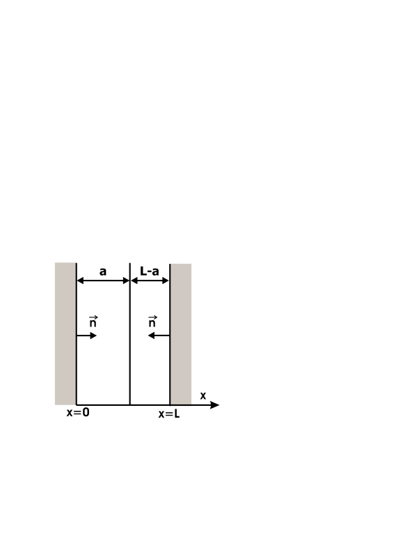
Figure 1: The Casimir piston in $x$ dimension

After the simple Majorana fermion piston, we shall examine the Majorana-fermion and vector-boson chamber and piston. The connection with supersymmetry shall be examined. In the case of Majorana-fermion and vector-boson (in the following fermion refers to Majorana fermion and boson to vector boson unless stated differently) piston we shall study three different cases, namely, fermion in one chamber ($a$-chamber) and boson in the other chamber ($L-a$-chamber), boson in the $a$-chamber and fermion in the $L-a$-chamber, and finally boson-fermion in the $a$-chamber and boson-fermion in the $L-a$-chamber (with different fermion flavors).

The motivation to use a piston with one chamber filled with a fermion and the other with boson, is even stronger. This comes from the fact that the Casimir energy density is regularized, and when the $L$ parameter is send to infinity, the Casimir energy yields the vector boson or Majorana fermion Casimir energy, of course without singularity. Thus this could be another regularization use of the piston with the new feature of using Majorana fermions and vector bosons. This could be particularly interesting since we can use a fermion just to regularize the vector boson field (photon) Casimir energy and then forget it. The new result within these considerations is that Casimir energy density (and therefore the Casimir energy) is regularized and not just the force. The motivation to study fermion boson chamber is the automatic cancelation of the singularities when the number of fermions and bosons follow the vector superfield rules dictated by supersymmetry. Of course supersymmetry is broken due to boundary conditions but a remnant of supersymmetry can be really useful.

We shall extend the boson fermion chambers and pistons in the case where the fermion obeys chiral boundary conditions on the plates. In that case the minimization of the energy as a function of the chiral parameter $\phi$ is examined. Also the sign of the Casimir force as a function of $\phi$ is also studied. Our next step will be to introduce two real scalar bosons, obeying Robin boundary conditions, and a massive Dirac fermion obeying bag boundary conditions. Although the number of the fields are determined by the supersymmetric chiral superfield rules, supersymmetry is broken due to boundary conditions. In that case the total Casimir energy can be zero in some cases

Finally we shall examine the massive scalar bosons Casimir effect between parallel plates in the case that mixed boundary conditions are imposed. The connection of this case with the rest of the present study is that the singularities cancel also. Indeed if one uses a boson, satisfying Dirichlet-Neumann boundary conditions on the plates, together with a scalar boson, satisfying Dirichlet-Dirichlet boundary conditions, the singularities of the Casimir energies for each case cancel each other.

Finally, we present the conclusions and we discuss some applications of the above study.

1 Majorana Fermions in a Slab and Bag Boundary
Conditions

Consider Majorana fermion fields in 3 space dimensions while one dimension is considered finite by two parallel plates at $x=0$ and $x=L$. We shall also assume that fermions are not allowed to exist outside the parallel plate system. This is actually the MIT bag boundary conditions which are expressed as

$$in^{\mu}\gamma_{\mu}\psi=\psi$$ (1)

or in Lorentz covariant form

$$n^{\mu}\bar{\psi}\gamma_{\mu}\psi=0$$ (2)

which $n^{\mu}=(0,\vec{n})$ and $\vec{n}$ the vector normal to the surface of the plates and directed to the interior of the slab configuration. The above two equations show that there is no fermion current flowing outwards of the parallel plates.

In most of the calculations we shall perform in this article we shall use the cutoff method [3, 7] in order to compute the Casimir energy, since we want to see explicitly the singularities that the Casimir energy has. The eigenvalues of the massless Dirac equation obeying bag boundary conditions are

$$\omega_{n}=\sqrt{k_{T}^{2}+\frac{\pi^{2}(n+\frac{1}{2})^{2}}{L^{2}}}$$ (3)

where $k_{T}$ refer to the transverse components of the momentum. Using the cutoff method the Casimir energy density per unit area reads [7],

$$\frac{\mathcal{E}_{f}}{L}=-\frac{1}{2L}2\sum_{n=0}^{\infty}\int\frac{\mathrm{d}^{2}k_{T}}{(2\pi)^{2}}{\,}\omega_{n}{\,}e^{-\tau\omega_{n}}$$ (4)

where $\mathcal{E}_{f}$ is the total Casimir energy per unit area between the plates and we have introduced an exponential regulator in terms of the cutoff $\tau$. The factor 2 for the Majorana fermion comes from the spin and the degrees of freedom in four spacetime dimensions. Using

$$\omega e^{-\omega\tau}=\big{(}\frac{\partial}{\partial\tau}\big{)}^{2}\big{(}\frac{1}{\omega}e^{-\omega\tau}\big{)}$$ (5)

and carrying out the integration we obtain

$$\frac{\mathcal{E}_{f}}{L}=-\frac{2}{L}\big{(}\frac{\partial}{\partial\tau}\big{)}^{2}\frac{1}{2\pi\tau}\Big{(}\frac{e^{-\frac{\pi\tau}{2L}}}{1-e^{-\frac{\pi\tau}{L}}}\Big{)}$$ (6)

In the limit $\tau\rightarrow 0$ we obtain

$$\frac{\mathcal{E}_{f}}{L}=-\frac{7}{8}\frac{\pi^{2}}{720{\,}L^{4}}-\frac{3}{\pi^{2}\tau^{4}}$$ (7)

where we can see explicitly the singularity in terms of the cutoff $\tau$. Note that the series over $\tau$ contains only even powers of $\tau$. This is a characteristic of fermions and vector bosons. Consistent boundary conditions for massless vector bosons are the so-called perfect conductor boundary conditions on the plates, namely

$$n_{\mu}F_{a}^{\mu{\,}\nu}=0$$ (8)

Working in the same way as in the fermion case, the Casimir energy density per unit area of a vector field satisfying perfect conductor boundary conditions on the plates reads

$$\frac{\mathcal{E}_{b}}{L}=\frac{1}{2L}\Big{(}2\sum_{n=1}^{\infty}\int\frac{\mathrm{d}^{2}k_{T}}{(2\pi)^{2}}{\,}\omega_{nb}{\,}e^{-\tau\omega_{nb}}+\int\frac{\mathrm{d}^{2}k_{T}}{(2\pi)^{2}}{\,}|k_{T}|{\,}e^{-\tau|k_{T}|}\Big{)}$$ (9)

where $\omega_{nb}=\sqrt{k_{T}^{2}+\frac{\pi^{2}n^{2}}{L^{2}}}$. Upon integration we obtain

$$\frac{\mathcal{E}_{b}}{L}=-\frac{1}{L}\big{(}\frac{\partial}{\partial\tau}\big{)}^{2}\frac{1}{2\pi\tau}\Big{(}\frac{1+e^{-\frac{\pi\tau}{L}}}{1-e^{-\frac{\pi\tau}{L}}}\Big{)}$$ (10)

and in the limit $\tau\rightarrow 0$ we obtain

$$\frac{\mathcal{E}_{b}}{L}=\frac{3}{\pi^{2}\tau^{4}}-\frac{1}{720}\frac{\pi^{2}}{L^{4}}$$ (11)

where $\mathcal{E}_{b}$ is the total Casimir energy per unit area of the boson between plates. We shall make extensive use of the above well known expressions in the rest of the paper (for a similar analysis see [25]). Note again that the series over $\tau$ contains even powers only, just as in the fermion case. For completeness we shall present briefly the scalar boson case. The scalar boson Casimir energy density reads

$$\frac{\mathcal{E}_{\mathrm{scalar}}}{L}=\frac{1}{2L}\sum_{n=1}^{\infty}\int\frac{\mathrm{d}^{2}k_{T}}{(2\pi)^{2}}{\,}\omega_{nb}{\,}e^{-\tau\omega_{nb}}$$ (12)

and after integrating, we obtain

$$\frac{\mathcal{E}_{\mathrm{scalar}}}{L}=\frac{1}{L}\big{(}\frac{\partial}{\partial\tau}\big{)}^{2}\frac{1}{\pi\tau}\Big{(}\frac{1}{-1+e^{\frac{\pi\tau}{L}}}\Big{)}$$ (13)

In the limit $\tau\rightarrow 0$, the Casimir energy density for the scalar field reads

$$\frac{\mathcal{E}_{\mathrm{scalar}}}{L}=\frac{6}{\pi^{2}\tau^{4}}-\frac{1}{L\pi\tau^{3}}-\frac{1}{720}\frac{\pi^{2}}{L^{4}}$$ (14)

It is obvious, contrary to the fermion and vector boson case, the scalar boson energy density contains even and odd powers of $\tau$.

2 Different Flavor Fermionic Casimir Piston

Let us see how the piston configuration that we mentioned in the introduction helps in the cancellation of the singularities. Consider a piston with two chambers that are constructed by three parallel plates at $x=0$, $x=a$ and $x=L$. The total Casimir energy per unit area of a Majorana fermion is equal to,

$$\mathcal{E}_{piston}=\mathcal{E}_{f}(a)+\mathcal{E}_{f}(L-a)$$ (15)

and relation (7) gives

$$\mathcal{E}_{piston}=-\frac{3a}{\pi^{2}\tau^{4}}-\frac{1}{720}\frac{\pi^{2}}{8{\,}a^{3}}-\frac{3(L-a)}{\pi^{2}\tau^{4}}-\frac{1}{720}\frac{\pi^{2}}{8{\,}(L-a)^{3}}$$ (16)

Taking the derivative of the total Casimir energy per unit area we obtain the Casimir force per unit area

$$F_{c}=-\frac{\partial\mathcal{E}_{piston}}{\partial a}$$ (17)

which is equal to

$$F_{c}=-\frac{3}{\pi^{2}\tau^{4}}-\frac{3}{720}\frac{\pi^{2}}{8{\,}a^{4}}+\frac{3}{\pi^{2}\tau^{4}}+\frac{3}{720}\frac{\pi^{2}}{8{\,}(L-a)^{4}}$$ (18)

In the above relation it is clear that the total Casimir force per unit area is finite.

Relation (18) is the Casimir force on a piston plate in the case the chambers are filled with different flavors of fermions (in order bag conditions are consistently fulfilled). Vacuum fluctuations of massless fermions between two parallel and confining plates give rise to an attractive Casimir force. Thus both vector bosons and fermions lead to a negative Casimir force, contrary to what would be expected from fermions due to Fermi-Dirac statistics. The Casimir force behaves exactly as in the bosonic case. In detail the force is attractive when $a$ is small and repulsive when $L-a$ is small (see also [9, 10, 11, 12, 13, 14, 15, 16, 17, 18, 19, 20]). Finally, it is obvious that in the limit $L\rightarrow\infty$ we obtain the usual Majorana fermionic Casimir force between plates (see [23, 24]).

3 Majorana Fermion-Vector Boson Chambers and Piston Configurations

Consider massless, non interacting vector bosons and Majorana fermions, described by the Lagrangian,

$$\mathcal{L}=-\frac{1}{4}F_{\mu{\,}\nu}F^{\mu{\,}\nu}+i\overline{\Psi}\gamma^{\mu}\partial_{\mu}\Psi,$$ (19)

We shall assume that the vector boson field and the Majorana fermion co-exist between two parallel plates located at $x=0$ and $x=L$. Thus we construct a chamber filled with bosons and fermions in a “supersymmetric” way. Indeed Lagrangian (19) looks like the $N=1$, $d=4$ vector supersymmetric Lagrangian describing photons and the supersymmetric partner, the photino. We should clarify at this point that supersymmetry is broken when the bag boundary conditions for fermions and perfect conductor boundary conditions are used for bosons on the plates. Thus in this physical system, supersymmetry is explicitly broken. A similar effect happens when physical systems are studied at finite temperature, where supersymmetry breaks due to different boundary conditions applied to bosons and fermions. However in the slab case there exists a remnant of supersymmetry. In fact we shall use the above Lagrangian in order to determine formally the appropriate number of fermions and bosons fields we should use for singularity cancellation.

3.1 Massless Vector Boson-Majorana Fermion Chamber

Consider one vector boson and one Majorana fermion field described by the Lagrangian (19). We assume that the fields are confined between two parallel plates on which fermions satisfy bag boundary conditions and bosons satisfy perfect conductor, that is

$$n^{\mu}\bar{\Psi}(x=0)\gamma_{\mu}\Psi(x=0)=0,\qquad\qquad{\,}n^{\mu}\bar{\Psi}(x=L)\gamma_{\mu}\Psi(x=L)=0$$ (20)

for fermions and

$$n_{\mu}F_{a}^{\mu{\,}\nu}=0$$ (21)

for vector bosons. The total Casimir energy per unit area of the slab system reads (Casimir slab chamber)

$$\mathcal{E}_{\mathrm{total}}=-\frac{1}{720}\frac{\pi^{2}}{L^{3}}+\frac{3L}{\pi^{2}\tau^{4}}-\frac{7}{720}\frac{\pi^{2}}{8L^{3}}-\frac{3L}{\pi^{2}\tau^{4}}$$ (22)

It is obvious that the Casimir energy per unit area for the plate chamber is singularity free, since the singularity of the fermion energy is canceled by the corresponding ones of the two bosons. This is a very valuable result and it is due to the supersymmetry remnant that the system possesses. The total Casimir force per unit area between the plates is

$$F_{\mathrm{total}}=-\frac{21}{720}\frac{\pi^{2}}{8L^{4}}-\frac{3}{720}\frac{\pi^{2}}{L^{4}}$$ (23)

which, as we can see, is attractive. Thus, when we consider the fermion boson chamber, the force between the plates is even more attractive compared to the single boson (fermion) case. It is not difficult to extend the chamber to a piston configuration, just to see how the force behaves. Of course each chamber is singularity free. Thus adding the contributions from the two chambers, $a$ and $L-a$, we obtain, the total Casimir energy (it is assumed that each chamber contains different fermion flavor)

$$\mathcal{E}_{\mathrm{total}}=-\frac{1}{720}\frac{\pi^{2}}{\alpha^{3}}-\frac{7}{720}\frac{\pi^{2}}{8\alpha^{3}}-\frac{1}{720}\frac{\pi^{2}}{(L-\alpha)^{3}}-\frac{7}{720}\frac{\pi^{2}}{8(L-\alpha)^{3}}$$ (24)

and the total Casimir force per unit area is given by

$$F_{\mathrm{total}}=-\frac{21}{720}\frac{\pi^{2}}{8\alpha^{4}}-\frac{3}{720}\frac{\pi^{2}}{\alpha^{4}}+\frac{21}{720}\frac{\pi^{2}}{8(L-\alpha)^{4}}+\frac{3}{720}\frac{\pi^{2}}{(L-\alpha)^{4}}$$ (25)

Notice that in the limit $L\rightarrow\infty$ relation (25) becomes identical to relation (23). Thus we recover the initial system, as is expected in every piston configuration.

4 Massless Boson-Fermion Piston.
A Regularization Method of the Casimir Energy Density per Unit Area Using the Piston

As we mentioned in the introduction, the most theoretically attractive feature of the piston is that it renders the Casimir force of a bosonic (and fermionic) system finite. However the Casimir energy density (and therefore the total Casimir energy) for the aforementioned fields, even for the piston configuration, contain singularities. We shall demonstrate a use that the Casimir piston offers to the regularization of the Casimir energy density. We will make use of the Casimir piston configuration but we shall fill the two chambers with different statistics fields. To be specific, consider that the $a$ chamber is filled with a Majorana fermion with bag boundary conditions on the boundaries while the $L-a$ chamber is filled with a vector boson satisfying perfect conductor boundary conditions on the two plates. Notice that the system as a whole is determined by the Lagrangian (19), so there is a remnant supersymmetry, which is however broken since the fields are confined in different places in space, and of course the boundary conditions are different. The fermionic Casimir energy energy density per unit area is equal to

$$\mathcal{U}_{f}(\alpha)=-\frac{7}{720}\frac{\pi^{2}}{8\alpha^{4}}-\frac{3}{\pi^{2}\tau^{4}}$$ (26)

while the vector boson has Casimir energy density

$$\mathcal{U}_{b}(L-a)=\frac{3}{\pi^{2}\tau^{4}}-\frac{1}{720}\frac{\pi^{2}}{(L-\alpha)^{4}}$$ (27)

The total Casimir energy density for the piston system is $\mathcal{U}_{total}=\mathcal{U}_{f}(a)+\mathcal{U}_{b}(L-a)$. Adding the above two contributions notice that the total Casimir energy density is finite, and equal to

$$\mathcal{U}_{total}=-\frac{1}{720}\frac{\pi^{2}}{(L-\alpha)^{4}}-\frac{7}{720}\frac{\pi^{2}}{8\alpha^{4}}$$ (28)

In the above relation, the total Casimir energy density behaves as follows,

$$\mathcal{U}_{total}=\bigg{\{}\begin{array}[]{c}\mathcal{\bar{U}}_{f}\quad\textrm{for}\quad 0\leq x\leq a\\ \mathcal{\bar{U}}_{b}\quad\textrm{for}\quad a\leq x\leq L\\ \end{array}$$ (29)

where $\bar{\mathcal{U}}_{f}$ is the regularized Majorana fermion energy density and $\bar{\mathcal{U}}_{b}$ is the corresponding one for the vector boson. Therefore, the energy density in each chamber is made regular and, of course, the total energy density is regular. The total fermionic Casimir energy density per unit area is equal to [28],

$$E_{f}(a)=\int_{0}^{a}\bar{\mathcal{U}}_{f}(a)\mathrm{d}x=-\frac{7}{720}\frac{\pi^{2}}{8\alpha^{3}}$$ (30)

since the fermionic energy density is regularized and independent of $x$. In the same way the vector boson total Casimir energy density per unit area is,

$$E_{b}(L-a)=\int_{a}^{L}\bar{\mathcal{U}}_{b}(a)\mathrm{d}x=-\frac{1}{720}\frac{\pi^{2}}{(L-\alpha)^{3}}$$ (31)

Adding the two bosons and fermion contributions we obtain the total Casimir energy of the piston

$$\mathcal{E}_{\mathrm{total}}=-\frac{1}{720}\frac{\pi^{2}}{(L-\alpha)^{3}}-\frac{7}{720}\frac{\pi^{2}}{8\alpha^{3}}$$ (32)

We can clearly see that the total Casimir energy is free of singularities since we regularized the Casimir energy density. By taking the limit $L\rightarrow\infty$ the total Casimir energy becomes equal to the single Majorana fermion Casimir energy. Thus the piston offers a regularization method for the fermion Casimir energy (and more importantly for the vector boson). This was the motivation to study such configurations. Of course the total Casimir force on the piston plate is regularized and free of singularities. Indeed, since $F=-\frac{\partial E}{\partial a}$, taking the derivative of (32) with respect to $a$, we obtain,

$$F_{\mathrm{total}}=\frac{3}{720}\frac{\pi^{2}}{(L-\alpha)^{4}}-\frac{21}{720}\frac{\pi^{2}}{8\alpha^{4}}$$ (33)

Again in limit $L\rightarrow\infty$ we render the usual fermionic Casimir force between plates with bag boundary conditions, divided by 2 due to the Majorana degrees of freedom [23, 24, 26, 27].

The most important case comes when in the above piston setup the fields are confined in the chambers with inverse order, that is, vector boson in the $a$ chamber and Majorana fermions in the $L-a$ chamber. Following the same procedure as in the previous, we obtain the total Casimir energy

$$\mathcal{E}_{\mathrm{total}}=-\frac{1}{720}\frac{\pi^{2}}{\alpha^{3}}-\frac{7}{720}\frac{\pi^{2}}{8(L-\alpha)^{3}}$$ (34)

and the total Casimir force,

$$F_{\mathrm{total}}=\frac{21}{720}\frac{\pi^{2}}{8(L-\alpha)^{4}}-\frac{3}{720}\frac{\pi^{2}}{\alpha^{4}}$$ (35)

It is obvious that the total Casimir energy is again singularity free, as was in the previous case. The difference of the two cases is that in the limit $L\rightarrow\infty$, the total Casimir energy becomes the Casimir energy of a massless vector boson field confined between two plates. Thus the inverse piston configuration serves as a regularization technique for the vector boson Casimir energy. Of course the force is finite, as we can see (35). The new regularization that the piston offers within the setup we presented is that the total energy is finite and not just the force.

In conclusion, the piston can offer a regularization method for the vector boson and Majorana fermion Casimir energy when we make use of a “supersymmetric” system in which fermions and bosons are put in different chambers. Although supersymmetry is broken due to boundary conditions, the singularities cancel in a supersymmetric way, and the Casimir energy is singularity free. In the limit $L\rightarrow\infty$ we render the known results. The new result in this use of piston is that the Casimir energy is regularized explicitly and not just the force.

5 Fermions-Bosons with Chiral Boundary Conditions

Apart from the bag boundary conditions on the plates that can be used for fermions, in the massless case we can use the so-called chiral boundary conditions. This stems from the invariance of the massless Dirac equation

$$\mathcal{L}=\mathrm{i}\bar{\psi}\gamma^{\mu}\partial_{\mu}\psi$$ (36)

under the transformation,

$$\psi^{\prime}=\exp(\mathrm{i}\gamma_{5}\beta)\psi$$ (37)

where $\beta$ is an arbitrary phase. The bag boundary conditions

$$\mathrm{i}n^{\mu}\gamma_{\mu}\psi=\psi$$ (38)

make the fermion current vanish outside the surface of the plates

$$n^{\mu}\bar{\psi}\gamma_{\mu}\psi=0$$ (39)

Although relation (39) is chirally invariant, the boundary condition (38) is not [27]. The restoration of the chiral symmetry in the boundary conditions can be achieved through the so called chiral boundary conditions,

$$\mathrm{i}n^{\mu}\gamma_{\mu}\psi=\exp(\mathrm{i}\gamma_{5}\phi)\psi$$ (40)

These conditions are invariant under the transformation (37) with $\phi$, being promoted to a dynamical variable, transforming as $\phi\rightarrow\phi-2\beta$.

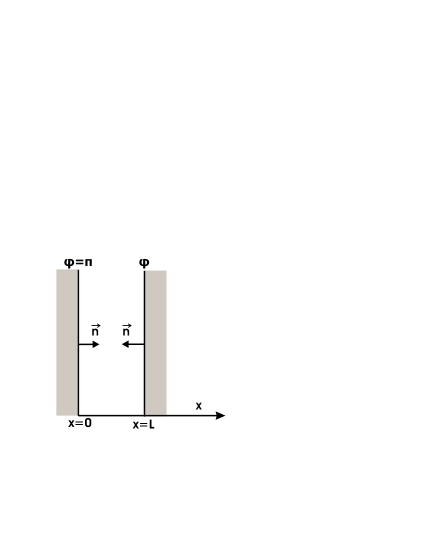
Figure 2: The chiral boundary conditions

Consider a chamber made from two parallel plates containing one vector boson gauge field satisfying perfect conductor boundary conditions on the plate and one Majorana fermion satisfying chiral boundary conditions on the plates. Regarding the chiral boundary conditions the $\phi$ parameter is considered to be $\phi=\pi$ on the plate located at $x=0$ and a general value $\phi$ on the other plate on $x=\alpha$ (with $0\leq\phi\leq 2\pi$). The reason to consider this setup is to examine the behavior of the Casimir energy and of the Casimir force as a function of the chiral parameter $\phi$. Moreover we want to examine the minimum of the energy as a function of $\phi$. It is known from reference [27], that the minimum energy for a fermion with chiral boundaries is obtained for $\phi=\pi$. We want to see how this result changes when we consider bosons and fermions together, in a “supersymmetric” way. (keeping in mind that chiral boundaries break supersymmetry. The motivation using bosons and fermions is as before, the cancellation of the singularities in the Casimir energy and consequently in the Casimir force, without the introduction of counter-terms to cancel the singularities.

The vector boson contribution to the total Casimir energy per unit area in the chamber is,

$$\mathcal{E}_{b}(\alpha)=-\frac{\pi^{2}}{720\alpha^{3}}+\frac{3a}{\pi^{2}\tau^{4}}$$ (41)

The fermionic Casimir energy per unit area with chiral boundaries reads,

$$\mathcal{E}_{f}(\alpha)=\frac{\pi^{2}}{720\alpha^{3}}-\frac{\phi^{2}}{384\pi^{2}\alpha^{3}}(\phi-2\pi)^{2}-\frac{3a}{\pi^{2}\tau^{4}}$$ (42)

Adding the two bosons and one fermion contributions we obtain the total Casimir energy in the chamber,

$$\mathcal{E}_{\mathrm{total}}=-\frac{\phi^{2}}{384\pi^{2}\alpha^{3}}(\phi-2\pi)^{2}$$ (43)

which is regular since the singularities of the two cancel each other. From the above we easily obtain the Casimir force between the plates,

$$F_{\mathrm{total}}=-\frac{\phi^{2}}{64\pi^{2}\alpha^{4}}(\phi-2\pi)^{2}$$ (44)

Thus we see that in the Casimir chamber with chiral boundaries the total Casimir energy is regularized.

5.1 Casimir Piston with Chiral Boundaries

To complete the study of the chiral boundaries Majorana fermion-vector boson chamber, we shall consider a piston using the above combination of fields and boundary conditions. Particularly suppose that we have a piston filled in the left chamber with a Majorana fermion obeying chiral boundary conditions on $x=0$ and $x=a$ (with $\phi=\pi$ on $x=0$ and general $\phi$ on $x=a$) and with a vector boson in the other chamber with perfect conductor boundary conditions at $x=a$ and $x=L$. Using the same procedure as in the piston configuration of section 4, we obtain the total Casimir energy, which is finite (free of singularities) and is equal to,

$$\mathcal{E}_{\mathrm{total}}=-\frac{\pi^{2}}{720(L-\alpha)^{3}}+\frac{\pi^{2}}{720\alpha^{3}}-\frac{\phi^{2}}{384\pi^{2}\alpha^{3}}(\phi-2\pi)^{2}$$ (45)

while the force on the plate at $x=a$ is given by

$$F_{\mathrm{total}}=\frac{\pi^{2}}{480\alpha^{4}}+\frac{\pi^{2}}{120(L-\alpha)^{4}}-\frac{\phi^{2}}{128\pi^{2}\alpha^{4}}(\phi-2\pi)^{2}$$ (46)

Notice that in the limit $L\rightarrow\infty$ the energy and the force become equal to that of a single Majorana fermion between plates with chiral boundary conditions.

A similar analysis holds for the case the boson and fermion are put into opposite chambers. In that case the energy is again finite of course and so is the force, which is equal to

$$F_{\mathrm{total}}=-\frac{\pi^{2}}{120\alpha^{4}}-\frac{\pi^{2}}{480(L-\alpha)^{4}}+\frac{\phi^{2}}{128\pi^{2}(L-\alpha)^{4}}(\phi-2\pi)^{2}$$ (47)

As before, the limit $L\rightarrow\infty$ renders the known result of vector boson force between two plates. Let us note that, as in the previous section, the regularization in the piston case occurs at the energy density per unit area.

6 Fermions with Bag Boundaries and Bosons with Robin Boundary Conditions

We discussed in the previous sections the case having massless Majorana fermions and vector bosons exist between parallel plates. The number of the fields we used was determined by the way they should appear in a vector supermultiplet of a $N=1$ supersymmetry. Of course supersymmetry was broken by the boundary conditions satisfied by fermions and bosons (bag or chiral for fermions and perfect conductor for bosons). Although supersymmetry was broken, the effect of using a vector boson and one Majorana fermion was that the singularities in the total Casimir energy per unit area (for the chamber) or in the Casimir energy density per unit area (for the piston case) where cancelled. In this section we shall consider a similar interplay between the number of fermions and bosons using two equal mass scalar bosons and a massive Dirac fermion. The boundary conditions will be bag for fermions and specific Robin boundary conditions for the scalar bosons.

To start with, consider a fermion between two parallel plates located at $x_{d}=0$ and $x_{d}=L$ embedded in a flat $d$-dimensional spacetime. The Casimir energy for the fermion equals to [7, 24]

$$\mathcal{E}_{f}=-C(d)\int\sum_{n}\frac{\mathrm{d}p^{d-2}}{(2\pi)^{d-2}}\sqrt{p^{2}+z_{n}^{2}+m_{f}^{2}}$$ (48)

with $C(d)=2^{(d-1)/2}$ for $d$ odd and $C(d)=2^{(d-2)/2}$ for $d$ even. When the fermion obeys bag boundary conditions in the two plates, the $z_{n}$ appearing above are solutions of the equation

$$F(z)=0$$ (49)

with

$$F(z)=mL\sin(z)+z\cos(z)$$ (50)

The roots of the above equation solve the eigenvalue problem for the massive slab bag fermion [7, 24].

Now consider a boson between two parallel plates located at $x_{d}=0$ and $x_{d}=L$ obeying robin boundary conditions [10, 33] of the form

$$(1+\beta_{1}\partial_{x})\phi(x,t)=0$$ (51)

on the first plate (at $x=0$) and

$$(1-\beta_{2}\partial_{x})\phi(x,t)=0$$ (52)

on the second plate ($\beta_{1,2}$ are arbitrary constants). Robin boundary conditions are known to provide conformal invariance for field theories between parallel plates [33] and are frequently used in the calculation of the Casimir energy (see [33, 10] and references therein). The interest in Robin boundary conditions comes from the fact that there is a region in the parameter space for which the Casimir forces are repulsive for small distances and attractive for large distances. Thus stabilization of the distance between the plates can be achieved.

We shall use Robin boundaries for the two massive scalar bosons between two parallel plates in a $d$ dimensional spacetime (the same setup as that of the fermion case). The Casimir energy for the system with these boundary conditions is obtained by solving the equation

$$F(y)=(1-b_{1}b_{2}y^{2})\sin y-(b_{1}+b_{2})y\cos y=0$$ (53)

with $b_{i}=\beta_{i}/L$. The above equation gives solution to the spectral problem under Robin boundary conditions [10, 33]. We shall use Dirichlet boundary conditions in the $x=0$ boundary (this means that $b_{1}=0$) and Robin boundary conditions on the $x=L$ boundary specified by,

$$b_{2}=-\frac{1}{mL}$$ (54)

Thus equation (53) reads

$$F(y)=mL\sin y+y\cos y=0$$ (55)

The solutions of this equation, namely the roots $y_{n}$, solves the spectral problem of the boson field between plates with boundary conditions (51) and (52). The bosonic Casimir energy of a massive boson reads

$$\mathcal{E}_{b}=\int\sum_{n}\frac{\mathrm{d}p^{d-2}}{(2\pi)^{d-2}}\sqrt{p^{2}+y_{n}^{2}+m_{b}^{2}}$$ (56)

Notice that equations (55) and (50) are identical. Thus the total Casimir energy for the two bosons and one fermion field equals to

$$\mathcal{E}_{tot}=2\mathcal{E}_{b}+\mathcal{E}_{f}=2\int\sum_{n}\frac{\mathrm{d}p^{d-2}}{(2\pi)^{d-2}}\sqrt{p^{2}+y_{n}^{2}+m_{b}^{2}}-C(d)\int\sum_{n}\frac{\mathrm{d}p^{d-2}}{(2\pi)^{d-2}}\sqrt{p^{2}+z_{n}^{2}+m_{f}^{2}}$$ (57)

The motivation to consider this fermion-boson “supersymmetric” configuration ($N=1$ chiral supermultiplet) is the observation that for $d=4$ and for $d=3$ the total Casimir energy vanishes when the fermion and bosons have the same mass, that is when $m_{f}=m_{b}$. This result holds only for these two $d$ values. Indeed, for $d=4$, the parameter $C(d)=2^{(d-2)/2}$ which holds for $d=$ even becomes $C(4)=2$. The same occurs for $d=3$ on the other relation. Thus although supersymmetry is broken on the boundaries, the total Casimir energy vanishes. This result is particularly interesting because it occurs only for $d=4$ when $d=$ even and $d=3$ when $d=$ odd. This effect is known to occur only in supersymmetric theories (see for example reference [40]).

7 Scalar Boson Piston with Neumann-Dirichlet-Dirichlet
Boundary Conditions

In this section we shall study a chamber filled with two scalar fields having the same mass. Although this differs only slightly from the case studied in the previous section, the motivation is to show another way to cancel the singularities from scalar bosons Casimir energies between two parallel plates. In order to see this, consider two scalar bosons in the space between two parallel plates located at $x=0$ and $x=L$. One of them is assumed to satisfy Dirichlet boundary conditions on both plates, while the other one satisfies Neumann at $x=0$ and Dirichlet on the other plate. Within the dimensional regularization method, the Casimir energy between the two plates of the Neumann-Dirichlet boson is equal to (in the end we shall put $d=4$ and $s=-1/2$)

$$\mathcal{E}_{ND}=\frac{1}{(2\pi)^{d-2}}\pi^{\frac{d-2}{2}}\frac{\Gamma(s-\frac{d-2}{2})}{\Gamma(s)}\sum_{n=0}^{\infty}\Big{[}\frac{\pi^{2}}{L^{2}}(n+\frac{1}{2})^{2}+m^{2}\Big{]}^{\frac{d-2}{2}-s}.$$ (58)

We shall use zeta-function regularization in order to compute the above. Making use of the following relation [4]

$$\sum_{n=0}^{\infty}\Big{(}a(n+\frac{1}{2})^{2}+q\Big{)}^{-s}=$$ (59)

$$-\sqrt{\frac{\pi}{a}}{\,}\frac{\Gamma(s-\frac{1}{2})}{\Gamma(s)}\frac{q^{-s+1/2}}{2}+\frac{2\pi^{s}q^{-s/2+1/4}a^{-s/2-1/4}}{\Gamma(s)}\sum_{n=1}^{\infty}(-1)^{n}n^{s-1/2}K_{s-1/2}(2\pi n\sqrt{\frac{q}{a}}).$$

the Casimir energy for the Neumann-Dirichlet scalar boson is

$$\mathcal{E}_{ND}=-\frac{1}{2^{d-1}\pi^{(d-1)/2}}\frac{\Gamma(s-\frac{d-1}{2})}{\Gamma(s)}(m^{2})^{-s+\frac{1}{2}+\frac{d-2}{2}}L$$ (60)

$$+\frac{2\pi^{s-(d-2)}}{\Gamma(s)}m^{\frac{1}{2}-(s-\frac{d-2}{2})}(\frac{\pi^{2}}{L^{2}})^{\frac{1}{4}-\frac{1}{2}(s-\frac{d-2}{2})}$$

$$\times(2mL)^{-s+\frac{d-1}{2}}\sum_{n=1}^{\infty}(-1)^{n}(2mLn)^{s-\frac{d-1}{2}}K_{s-\frac{d-1}{2}}(2mnL)$$

with

$$\sum_{n=1}^{\infty}(-1)^{n}(2mLn)^{s-\frac{d-1}{2}}K_{s-\frac{d-1}{2}}(2mnL)=$$ (61)

$$\sum_{n=1}^{\infty}(4mLn)^{s-\frac{d-1}{2}}K_{s-\frac{d-1}{2}}(4mnL)-\sum_{n=1}^{\infty}(2mLn)^{s-\frac{d-1}{2}}K_{s-\frac{d-1}{2}}(2mnL)$$

In the above, the following relation was used.

$$\sum_{q=1}^{\infty}(-1)^{q}f(r)=2\sum_{q=1}^{\infty}f(2r)-\sum_{q=1}^{\infty}f(r)$$ (62)

In the same way we obtain the Casimir energy of the Dirichlet-Dirichlet boson which is equal to

$$\mathcal{E}_{DD}=-\frac{1}{2^{d-1}\pi^{(d-2)/2}}\frac{\Gamma(s-\frac{d-2}{2})}{\Gamma(s)}m^{2}$$ (63)

$$+\frac{1}{2^{d-1}\pi^{(d-1)/2}}\frac{\Gamma(s-\frac{d-1}{2})}{\Gamma(s)}(m^{2})^{-s+\frac{1}{2}+\frac{d-2}{2}}L$$

$$+\frac{1}{2^{d-3}}\frac{\pi^{s-(d-2)}}{\Gamma(s)}m^{\frac{1}{2}-(s-\frac{d-2}{2})}(\frac{L^{2}}{\pi^{2}})^{\frac{1}{4}+\frac{1}{2}(s-\frac{d-2}{2})}$$

$$\times\sum_{n=1}^{\infty}n^{s-\frac{d-1}{2}}K_{s-\frac{d-1}{2}}(2mnL)$$

where we have made use of the following analytic continuation [4]

$$\zeta_{EH}(s;p)=-\frac{p^{-s}}{2}+\frac{\sqrt{\pi}{\,}{\,}\Gamma(s-1/2)}{2\Gamma(s)}p^{-s+1/2}+\frac{2\pi^{s}p^{-s/2+1/4}}{\Gamma(s)}\sum_{n=1}^{\infty}n^{s-1/2}K_{s-1/2}(2\pi n\sqrt{p}).$$ (64)

Thus the total Casimir energy between the plates is $\mathcal{E}_{tot}=\mathcal{E_{DD}}+\mathcal{E_{ND}}$. As can be easily seen, relations (63) and (60) contain singularities due to the Gamma function $\Gamma(s-\frac{d-1}{2})$ for $d=4$ and $s=-1/2$ (first line of (60) and second line of (63)). It is obvious that the two singular terms cancel each other, thus the final result of the total Casimir energy is finite. The final expression is equal to,

$$\mathcal{E}_{tot}=\frac{2\pi^{s-(d-2)}}{\Gamma(s)}m^{\frac{1}{2}-(s-\frac{d-2}{2})}(\frac{\pi^{2}}{L^{2}})^{\frac{1}{4}-\frac{1}{2}(s-\frac{d-2}{2})}$$ (65)

$$\times\Big{(}\sum_{n=1}^{\infty}(4mLn)^{s-\frac{d-1}{2}}K_{s-\frac{d-1}{2}}(4mnL)-\sum_{n=1}^{\infty}(2mLn)^{s-\frac{d-1}{2}}K_{s-\frac{d-1}{2}}(2mnL)\Big{)}$$

$$-\frac{1}{2^{d-1}\pi^{(d-2)/2}}\frac{\Gamma(s-\frac{d-2}{2})}{\Gamma(s)}m^{2}$$

$$+\frac{1}{2^{d-3}}\frac{\pi^{s-(d-2)}}{\Gamma(s)}m^{\frac{1}{2}-(s-\frac{d-2}{2})}(\frac{L^{2}}{\pi^{2}})^{\frac{1}{4}+\frac{1}{2}(s-\frac{d-2}{2})}$$

$$\times\sum_{n=1}^{\infty}n^{s-\frac{d-1}{2}}K_{s-\frac{d-1}{2}}(2mnL)$$

We shall not pursuit this further since we just wanted to show how the cancellation of singularities within this setup occurs in four dimensions.

8 Conclusions

We have studied the Casimir effect of a massless Majorana fermion field and of a massless vector boson field confined between parallel plates. Particularly we considered the vector boson and the fermion field contained in a chamber and in a piston. We used various configurations which we now briefly discuss. The way the fields where chosen was according to a $N=1$ supersymmetric Lagrangian that was actually broken due to the boundary conditions obeyed by the fields on the parallel plates. The fermion field was supposed to obey bag or chiral bag boundary conditions on the plates while the vector boson field obeyed perfect conductor boundary conditions.

We saw that when we use both massless Majorana fermions and vector bosons in a chamber, both the total Casimir energy density and the Casimir energy density per unit area is singularity free. We used the cutoff method in order to explicitly see this cancellation. Thus although supersymmetry was explicitly broken on the boundary of the parallel plate chamber, a remnant of supersymmetry was responsible for the cancellation of the singularities.

Another interesting configuration we used in this article was the piston, which consists of three parallel plates placed at $x=0$, $x=a$ and $x=L$. We have started by putting in the $a$ chamber the massless Majorana fermion and in the $L-a$ chamber the massless vector boson obeying bag and perfect conductor boundary conditions respectively. We concluded that the energy density per unit area of the system is regularized when we add the energy density contributions from the two chambers of the piston. Then integrating on the finite dimension we obtain the total energy per unit area for the piston. The limit $L\rightarrow\infty$ yields the fermionic Casimir energy density for a Majorana fermion. The Casimir force was calculated and in the limit $L\rightarrow\infty$ turns to be identical with the fermion Casimir force between two plates at a distance $a$.

Equally interesting is the case for which the vector boson is put in the $a$ chamber and the Majorana fermion on the $L-a$ chamber. We concluded that the energy density per unit area is regularized. As before we calculated the total Casimir energy and force which we found it to be finite. The limit $L\rightarrow\infty$ yield the Casimir force and Casimir energy for a vector boson between two parallel plates. We should mention that this method yields a regularized result at the energy density level and not just in the force level.

The interest in calculating massless vector boson Casimir energies is obvious, since the photon belongs to that category. Thus the confinement of the electromagnetic field in a slab leads to a quantum effect, a vacuum energy density. We regularized the vacuum energy density using a massless Majorana fermion in the other chamber. That Majorana particle could be the photino.

The calculation of Majorana fermion Casimir energy densities is well motivated. Majorana fermions occur quite frequently in various research areas of physics. For example in some models of universal extra dimensions, a WIMP candidate (Weakly Interacting Massive Particle) is the Kaluza-Klein neutrino (the universal extra dimensions Kaluza-Klein excitation) which is a Majorana fermion [41]. Actually the Dirac neutrino is experimentally ruled out since the Z-induced neutron coherent contribution would be too large, which does not happen in the Majorana case. Another interesting appearance of Majorana fermion states comes from the physics of superconductors and superfluids. Particularly a Majorana bound state is theoretically predicted in rotating superfluid ${}^{3}\mathrm{He-A}$ between parallel plates. In the parallel plate geometry, the gap is about $10\mu$m and a Magnetic field is applied along the plates. The Majorana vortex bound state is associated with a singular vortex in chiral p-wave superfluid [42]. Similar studies show that a Majorana bound state exists in triplet superconductors (see [43]).

Concluding on the Majorana-vector boson case, the chamber and the piston setups where extended to the case of a fermion field obeying chiral bag boundary conditions and we have found that similar results hold.

Following the same supersymmetric recipe, regarding the number of fields (of course supersymmetry is broken on the boundaries), we studied a massive Dirac fermion and two massive scalar bosons between two parallel plates. The spacetime dimensions is $d$ and the fermions obey bag boundary conditions on the plates, while the scalar bosons obey specific Robin boundary conditions. We found that for $d=4$ (for $d=$ even) and for $d=3$ (for $d=$ odd) when the fermions and bosons have the same mass, the total Casimir energy vanishes. It is interesting to note that this occurs only for $d=3,4$.

Finally we presented another case in which the singularities of the Casimir energy cancel. It is Casimir chamber filled with two massive scalar bosons obeying Neumann and Dirichlet boundary conditions at the plates. We found that under these circumstances the Casimir energy of the system is singularity free.

Regarding the Majorana-vector boson case, it would be interesting to include finite temperature corrections or constant magnetic field in the calculation of the Casimir energy. This is of particular importance since these situations occur in nano-devices and in other technological applications where Majorana fermions appear [42].

References

- [1] H. Casimir, Proc. Kon. Nederl. Akad. Wet. 51 793 (1948)
- [2] T.H. Boyer, Phys. Rev. 174 (1968) 1764.
- [3] M. Bordag, U. Mohideen, V. M. Mostepanenko, Phys. Rep. 353, 1 (2001); E. Elizalde, J. Phys. A41, 304040 (2008); E. Elizalde, J. Phys. A39, 6299 (2006); E. Elizalde, A. Romeo, J. Math. Phys. 30, 1133 (1989); Michael Bordag, E. Elizalde, K. Kirsten, S. Leseduarte, Phys. Rev. D56, 4896 (1997); S. D. Odintsov, I. L. Buchbinder, Fortsch. Phys. 37, 225 (1989); K. Milton, Phys. Rev. D22, 1444 (1980); K. Milton, Phys. Rev. D22, 1441 (1980)
- [4] E. Elizalde, ”Ten physical applications of spectral zeta functions”, Springer (1995); E. Elizalde, S. D. Odintsov, A. Romeo, A. A. Bytsenko, S. Zerbini, ”Zeta regularization techniques and applications”, World Scientific (1994)
- [5] J. Ambjorn and S. Wolfram, Ann. Phys. 147, 1 (1983)
- [6] A. Chodos, R. L. Jaffe, K. Johnson, C. B. Thorn, V. F. Weisskopf, Phys. Rev. D9, 3471 (1974)
- [7] K. Johnson, Act. Phys. Polonica, B6, 865 (1975)
- [8] R. M. Cavalcanti, Phys. Rev. D69, 065015 (2004)
- [9] K. Kirsten, S. A. Fulling, Phys. Rev. D79, 065019 (2009)
- [10] E. Elizalde, S. D. Odintsov, A. A. Saharian, Phys. Rev. D79, 065023 (2009)
- [11] S. A. Fulling, K. Kirsten, Phys. Lett. B. 671, 179 (2009)
- [12] S. A. Fulling, J. H. Wilson, quant-ph/0608122
- [13] H. Cheng, Phys. Lett. B. 668, 72 (2008)
- [14] A. Edery, Phys. Rev. D75, 105012 (2007)
- [15] A. Edery, J. Phys. A39, 685 (2006)
- [16] A. Edery, V. Marachevsky, Phys. Rev. D78, 025021 (2008)
- [17] A. Edery, I. MacDonald, JHEP 09, 005 (2007)
- [18] L. P. Teo, Phys. Lett. B672, 190 (2009)
- [19] L. P. Teo, Nucl. Phys. B819, 431 (2009)
- [20] S. C. Lim, L. P. Teo, Eur. Phys. J. C60, 323 (2009)
- [21] V. K. Oikonomou, Mod. Phys. Lett. A24, 2405 (2009)
- [22] N. Graham, R. Jaffe, V. Khemani, M. Quandt, O. Schroeder, H. Weigel, Nucl. Phys. B677, 379 (2004)
- [23] R. D. M. Paola, R. B. Rodrigues, N. F. Svaiter, Mod. Phys. Lett. A14, 2353 (1999)
- [24] E. Elizalde, F. C. Santos, A. C. Tort, Int. J. Mod. Phys. A18, 1761 (2003)
- [25] H. Abe, J. Hashida, T. Muta, A. Purwanto, Mod. Phys. Lett. A14, 1033 (1999)
- [26] S. A. Gundersen, F. Ravndal, Ann. Phys. 182, 90 (1988)
- [27] C. A. Lutken, F. Ravndal, J. Phys. G. 10, 123 (1984)
- [28] S. A. Fulling, Aspects of quantum field theory in curved space-time CUP (1989)
- [29] S. C. Lim, L. P. Teo, arXiv:0807.3631
- [30] Xiang-Huazhai, Yan-Yanzhang, Xin-Zhouli, Mod. Phys. Lett. A24:, 393 (2009)
- [31] X.-H. Zhai, X.-Z. Li, Phys. Rev. D76, 047704 (2007)
- [32] V. Marachevsky, Phys. Rev. D75, 085019 (2007)
- [33] A. Romeo, A. A. Saharian, J. Phys. A35, 1297 (2002)
- [34] S. Bellucci, A. A. Saharian, Phys. Rev. D80, 105003 (2009)
- [35] K. Kirsten, J. Math. Phys. 35, 459-470 (1994)
- [36] E. Elizalde, A. Romeo, Phys. Rev. D40, 436 (1989); Michael Bordag, E. Elizalde, K. Kirsten, S. Leseduarte, Phys. Rev. D56, 4896 (1997); E. Elizalde, A. Romeo, J. Math. Phys. 30, 1133 (1989); Michael Bordag, E. Elizalde, K. Kirsten, J. Math. Phys. 37, 895 (1996); E. Elizalde, Michael Bordag, K. Kirsten, J. Phys. A31, 1743 (1998)
- [37] K. Kirsten, J. Math. Phys. 32, 3008-3014 (1991)
- [38] A.A. Bytsenko, E. Elizalde, S. Zerbini, Phys. Rev. D64, 105024 (2001); E. Elizalde, Commun. Math. Phys. 198, 83 (1998); E. Elizalde, J. Phys. A34, 3025 (2001)
- [39] I.S. Gradshteyn and I.M. Ryzhik, Table of Integrals Series and Products (Academic Press, 1965)
- [40] Y. Igarashi, Phys. Rev. D30, 1812 (1984)
- [41] V. K. Oikonomou, J. D. Vergados, Ch. Moustakidis, Nucl. Phys. B773, 19 (2007)
- [42] Y. Tsutsumi, T. Kawakami, T. Mizushima, M. Ichioka, K. Machida, Phys. Rev. Lett. 101, 135302 (2008)
- [43] H. Y. Keep, A. Raghavan, K. Maki, arXiv:0711.0929