Heavy quark effects on parton distribution functions in the unpolarized virtual photon up to the next-to-leading order in QCD

Abstract

We investigate the heavy quark mass effects on the parton distribution functions in the unpolarized virtual photon up to the next-to-leading order in QCD. Our formalism is based on the QCD-improved parton model described by the DGLAP evolution equation as well as on the operator product expansion supplemented by the mass-independent renormalization group method. We evaluate the various components of the parton distributions inside the virtual photon with the massive quark effects, which are included through the initial condition for the heavy quark distributions, or equivalently from the matrix element of the heavy quark operators. We discuss some features of our results for the heavy quark effects and their factorization-scheme dependence.

I Introduction

The CERN Large Hadron Collider (LHC) has restarted LHC and discoveries of signals for the new physics beyond the standard model (SM) are much anticipated. In order to fully complement the discoveries at LHC, we need more precise measurements which will be provided by the International Linear Collider (ILC), a proposed $e^{+}e^{-}$ collider machine ILC . In analyzing the signals for the new physics, it is still important for us to have a detailed knowledge of the SM predictions at high energies based on QCD.

In $e^{+}e^{-}$ collision experiments at high energies, the cross section of the two-photon processes $e^{+}e^{-}\rightarrow e^{+}e^{-}+{\rm hadrons}$ dominates over other processes such as the annihilation processes $e^{+}e^{-}\rightarrow\gamma^{*}\rightarrow{\rm hadrons}$. The two-photon processes provide a suitable testing ground for studying the QCD predictions at high energies. We consider here the two-photon processes in the double-tag events, where both the outgoing $e^{+}$ and $e^{-}$ are detected. In particular, we investigate the case in which one of the virtual photon is far off-shell (large $Q^{2}\equiv-q^{2}$), while the other is close to the mass-shell (small $P^{2}=-p^{2}$). Then the process can be viewed as a deep-inelastic scattering where the target is a photon rather than a nucleon twophoton (see Fig. 1). In this deep-inelastic scattering off photon targets, we can investigate the photon structure functions, which are the analogues of the nucleon structure functions. The study of the photon structure functions has long been an active field of research both theoretically and experimentally Review .

Figure 1: Deep inelastic scattering on a virtual photon in the $e^{+}~{}e^{-}$ collider experiments.

A unique and interesting feature of the photon structure functions is that, in contrast with the nucleon case, the target mass squared $P^{2}$ is not fixed but can take various values and that the structure functions show different behaviors depending on the values of $P^{2}$.

The unpolarized (spin-averaged) photon structure functions $F_{2}^{\gamma}(x,Q^{2})$ and $F_{L}^{\gamma}(x,Q^{2})$ of the real photon ($P^{2}=0$) were studied in the parton model QPM , in perturbative QCD (pQCD) by using the operator product expansion (OPE) CHM supplemented by the renormalization group (RG) method Witten ; BB and also by using the QCD improved PM Altarelli powered by the parton evolution equation Dewitt ; GR1983 ; MVV2002 ; MVV2004NNLOpart3 . The polarized photon structure function $g_{1}^{\gamma}(x,Q^{2})$ of the real photon was analyzed in pQCD polg1LO ; polg1NLO1 ; GRS2001 . The QCD analysis has been made for $F_{2}^{\gamma}(x,Q^{2})$ up to the next-to-next-to-leading order (NNLO) MVV2002 and for $g_{1}^{\gamma}(x,Q^{2})$ up to the next-to-leading order (NLO) polg1NLO1 ; GRS2001 .

For a virtual photon target ($P^{2}\neq 0$), we obtain the virtual photon structure functions $F_{2}^{\gamma}(x,Q^{2},P^{2})$ and $F_{L}^{\gamma}(x,Q^{2},P^{2})$. In fact, these structure functions were analyzed in pQCD for the kinematical region,

$$\Lambda^{2}\ll P^{2}\ll Q^{2}~{},$$ (1)

where $\Lambda$ is the QCD scale parameter UW1 ; UW2 ; Rossi ; BorzumatiSchuler ; Chyla . The advantage of studying a virtual photon target in this kinematical region (1) is that we can calculate the whole structure function, its shape and magnitude, by the perturbative method. This is contrasted with the case of the real photon target where in the NLO and beyond there appear nonperturbative pieces. With the recently calculated results of the three-loop anomalous dimensions of quark and gluon operators MVV2004NNLOpart1 ; MVV2004NNLOpart2 and also of the three-loop photon-quark and photon-gluon splitting functions MVV2004NNLOpart3 the virtual photon structure function $F_{2}^{\gamma}$ ($F_{L}^{\gamma}$) was investigated up to the NNLO (to the NLO) in pQCD USU2007 ; KSUU2008 . In the same kinematical region (1), the polarized virtual photon structure function $g_{1}^{\gamma}(x,Q^{2},P^{2})$ was studied in pQCD SU1999 ; GRS2001 ; BSU2002 ; SUU2006 .

In parton picture, structure functions are expressed as convolutions of coefficient functions and parton distribution functions (PDFs) in the target. The knowledge of these parton distributions is important since they will be used for predicting the cross sections of other inclusive processes. When the target is a virtual photon with $P^{2}$ being in the kinematical region (1), then a definite prediction can be made for its parton distributions in pQCD. The parton contents of the unpolarized and polarized virtual photon for this case were studied in Refs. Rossi ; DG ; GRStratmann ; Fontannaz ; SU2000 . Recently the QCD analysis of the parton distributions in the unpolarized virtual photon target was performed up to the NNLO USU2009 .

Although the photon structure functions and photonic parton distributions were studied in pQCD up to the NNLO MVV2002 ; USU2007 ; USU2009 , in these analyses all the contributing quarks were assumed to be massless. The production channel of a heavy flavor (with mass $m$) opens when $(p+q)^{2}\geq 4m^{2}$ and its mass effects should be taken into account unless $Q^{2}\gg m^{2}$. In fact the study of heavy quark mass effects for the two-photon processes and photon structure functions has appeared in the literature GR1983 ; GRV1992b ; GRStratmann ; Fontannaz ; GRS2001 ; AFG ; GRSch1999 ; SSU2002 ; CJKL2003 ; CJK2004 . Quite recently the present authors analyzed the heavy quark mass effects on $F_{2}^{\gamma}$ for the kinematical region (1) up to the NLO KSUU2009 using a different approach from the ones before. The analysis was made in the framework based on the QCD improved PM and the mass-independent RG equations, in which the RG equation parameters, i.e., $\beta$ and $\gamma$ functions, are the same as those for the massless quark case.

In this paper we examine the heavy quark mass effects on the parton distribution functions in the unpolarized virtual photon up to the NLO in pQCD. We use the same framework as the one in Ref. KSUU2009 , the QCD improved PM combined with the mass-independent RG equations. We consider the system which consists of $n_{f}-1$ light (i.e., massless) quarks and one heavy quark together with gluons and photons. Then, the heavy quark mass effects are included in the RG equation inputs; the coefficient functions and the operator matrix elements. In the case of the nucleon target, the heavy quark mass effects were studied by a method based on the OPE in Ref. Buza-etal1999 , where the heavy quark was treated such that it was radiatively generated and absent in the intrinsic quark components of the nucleon. This picture does not hold for the case of the photon, since the heavy quark is also generated from the photon target together with light quarks at high energies. We should consider both the heavy and light quarks equally as the partonic components inside the virtual photon.

In the next section, we derive the evolution equations for the parton distribution functions for the case where $n_{f}-1$ light quarks and one heavy quark are present. Then solving these equations, we give the explicit expressions up to the NLO for the moments of the light flavor singlet (nonsinglet) quark, heavy quark and gluon distributions. The parton distributions are dependent on the scheme which is employed to factorize structure functions into coefficient functions and parton distributions. We investigate the photonic parton distributions in two factorization schemes, namely $\overline{\rm MS}$ BBDM and ${\rm DIS}_{\gamma}$ GRV1992a schemes. In Sec. III, we enumerate all the necessary QCD parameters to evaluate the photonic parton distributions up to the NLO in $\overline{\text{MS}}$ scheme. The parton distributions in $\text{DIS}_{\gamma}$ scheme are considered in Sec. IV. The numerical analysis of the parton distributions predicted by $\overline{\rm MS}$ and ${\rm DIS}_{\gamma}$ schemes will be given in Sec. V. The final section is devoted to the conclusions. In Appendix A we consider the parton distributions in the virtual photon for the case when all $n_{f}$ quarks are light.

II Parton distributions in the virtual photon with a heavy quark flavor

We investigate the parton distributions in the virtual photon for the case when one heavy flavor quark appears together with $n_{f}-1$ light (i.e., massless) quarks. The analysis is made in the framework of the QCD improved parton model Altarelli powered by the DGLAP parton evolution equations. A part of the analysis was reported in Ref. KSUU2009 . Let

$$q^{i}_{L}(x,Q^{2},P^{2}),\qquad q^{\gamma}_{H}(x,Q^{2},P^{2}),\qquad G^{\gamma}(x,Q^{2},P^{2}),\qquad\Gamma^{\gamma}(x,Q^{2},P^{2}),$$ (2)

be light quark (with $i$-flavor and $i=1,\cdots,n_{f}-1$), heavy quark, gluon and photon distribution functions in the virtual photon with mass $-P^{2}$. Since the parton distributions in the photon are defined in the lowest order of the electromagnetic coupling constant, $\alpha=e^{2}/4\pi$, $\Gamma^{\gamma}$ does not evolve with $Q^{2}$ and is set to be $\Gamma^{\gamma}(x,Q^{2},P^{2})=\delta(1-x)$. In the light quark sector, it is more advantageous to treat, instead of using $q_{L}^{i}$, the “flavor singlet” and “nonsinglet” combinations $q^{\gamma}_{Ls}$ and $q^{\gamma}_{Lns}$ defined as follows:

$$q^{\gamma}_{Ls}\equiv\sum_{i=1}^{n_{f}-1}q^{i}_{L}~{},\qquad q^{\gamma}_{Lns}\equiv\sum_{i=1}^{n_{f}-1}e^{2}_{i}\Bigl{(}q^{i}_{L}-\frac{1}{n_{f}-1}q^{\gamma}_{Ls}\Bigr{)},$$ (3)

where $e_{i}$ is the electromagnetic charge of the $i$-flavor quark in the unit of proton charge.

Now introducing a row vector

$$\mbox{\boldmath$q$}^{\gamma}=\left(q^{\gamma}_{Ls},q^{\gamma}_{H},G^{\gamma},q^{\gamma}_{Lns}\right),$$ (4)

the parton distributions $\mbox{\boldmath$q$}^{\gamma}(x,Q^{2},P^{2})$ in the virtual photon satisfy the inhomogeneous DGLAP evolution equation Dewitt ; GR1983 ; MVV2002

$$\frac{d\mbox{\boldmath$q$}^{\gamma}(x,Q^{2},P^{2})}{d\ln Q^{2}}=\mbox{\boldmath$k$}(x,Q^{2})+\int_{x}^{1}\frac{dy}{y}\mbox{\boldmath$q$}^{\gamma}(y,Q^{2},P^{2})\hat{\mbox{\boldmath$P$}}\left(\frac{x}{y},Q^{2}\right),$$ (5)

where the elements of a row vector $\mbox{\boldmath$k$}=\left(k_{Ls},k_{H},k_{G},k_{Lns}\right)$ refer to the splitting functions of $\gamma$ to the light flavor-singlet quark combination, to heavy quark, to gluon and to light flavor-nonsinglet combination, respectively. The $4\times 4$ matrix $\hat{\mbox{\boldmath$P$}}\left(z,Q^{2}\right)$ is expressed as

$$\hat{\mbox{\boldmath$P$}}(z,Q^{2}) = \begin{pmatrix}P^{S}_{LL}(z,Q^{2})&P_{HL}(z,Q^{2})&P_{GL}(z,Q^{2})&0\\ P_{LH}(z,Q^{2})&P_{HH}(z,Q^{2})&P_{GH}(z,Q^{2})&0\\ P_{LG}(z,Q^{2})&P_{HG}(z,Q^{2})&P_{GG}(z,Q^{2})&0\\ 0&0&0&P^{NS}_{LL}(z,Q^{2})\\ \end{pmatrix},$$ (6)

where $P_{AB}$ is a splitting function of $B$-parton to $A$-parton.

The method to solve the above inhomogeneous DGLAP Eq. (5) is well known GR1983 . We sketch out the procedures. First we take the Mellin moments,

$$\frac{d\mbox{\boldmath$q$}^{\gamma}(n,Q^{2},P^{2})}{d\ln Q^{2}} = \mbox{\boldmath$k$}(n,Q^{2})+\mbox{\boldmath$q$}^{\gamma}(n,Q^{2},P^{2})\hat{\mbox{\boldmath$P$}}(n,Q^{2}),$$ (7)

where we have defined the moments of an arbitrary function $f(x)$ as $f(n)\equiv\int_{0}^{1}dxx^{n-1}f(x)$. Hereafter we omit the obvious $n$ dependence for simplicity. Then expansions are made for the splitting functions $\mbox{\boldmath$k$}(Q^{2})$ and $\hat{\mbox{\boldmath$P$}}(Q^{2})$ in powers of the QCD and QED coupling constants as

$$\mbox{\boldmath$k$}(Q^{2}) = \frac{\alpha}{2\pi}\mbox{\boldmath$k$}^{(0)}+\frac{\alpha\alpha_{s}(Q^{2})}{(2\pi)^{2}}\mbox{\boldmath$k$}^{(1)}+\cdots,$$ (8)

$$\hat{\mbox{\boldmath$P$}}(Q^{2}) = \frac{\alpha_{s}(Q^{2})}{2\pi}\hat{\mbox{\boldmath$P$}}^{(0)}+\left[\frac{\alpha_{s}(Q^{2})}{2\pi}\right]^{2}\hat{\mbox{\boldmath$P$}}^{(1)}+\cdots,$$ (9)

and a new variable $t$ is introduced as the evolution variable instead of $Q^{2}$ FP1 ,

$$t\equiv\frac{2}{\beta_{0}}\ln\frac{\alpha_{s}(P^{2})}{\alpha_{s}(Q^{2})}~{}.$$ (10)

The solution $\mbox{\boldmath$q$}^{\gamma}(t)(=\mbox{\boldmath$q$}^{\gamma}(n,Q^{2},P^{2}))$ of (7) is decomposed in the following form:

$$\mbox{\boldmath$q$}^{\gamma}(t)=\mbox{\boldmath$q$}^{\gamma(0)}(t)+\mbox{\boldmath$q$}^{\gamma(1)}(t)~{},$$ (11)

where the first and second terms represent the solution in the LO and NLO, respectively. Then they satisfy the following two differential equations:

$$\frac{d{\mbox{\boldmath$q$}}^{\gamma(0)}(t)}{dt} = \frac{\alpha}{\alpha_{s}(t)}{\mbox{\boldmath$k$}}^{(0)}+{\mbox{\boldmath$q$}}^{\gamma(0)}(t)P^{(0)}~{},$$ (12)

$$\frac{d{\mbox{\boldmath$q$}}^{\gamma(1)}(t)}{dt} = \frac{\alpha}{2\pi}\Bigl{[}{\bf k}^{(1)}-\frac{\beta_{1}}{2\beta_{0}}{\bf k}^{(0)}\Bigr{]}+\frac{\alpha_{s}(t)}{2\pi}{\mbox{\boldmath$q$}}^{\gamma(0)}(t)\Bigl{[}P^{(1)}-\frac{\beta_{1}}{2\beta_{0}}P^{(0)}\Bigr{]}+{\mbox{\boldmath$q$}}^{\gamma(1)}(t)P^{(0)}~{},$$ (13)

where we have used the fact the QCD effective coupling constant $\alpha_{s}(Q^{2})$ satisfies

$$\frac{d\alpha_{s}(Q^{2})}{d{\rm ln}Q^{2}}=-\beta_{0}\frac{\alpha_{s}(Q^{2})^{2}}{4\pi}-\beta_{1}\frac{\alpha_{s}(Q^{2})^{3}}{(4\pi)^{2}}+\cdots~{},$$ (14)

with $\beta_{0}=(11-\frac{2}{3}n_{f})$ and $\beta_{1}=(102-\frac{38}{3}n_{f})$. Note that the $P^{2}$ dependence of $\mbox{\boldmath$q$}^{\gamma}$ solely comes from the initial condition (or boundary condition) as we will see below.

The initial conditions for $\mbox{\boldmath$q$}^{\gamma(0)}$ and $\mbox{\boldmath$q$}^{\gamma(1)}$ are obtained as follows: for $-p^{2}=P^{2}\gg\Lambda^{2}$ the photon matrix elements of the hadronic operators $O^{n}_{i}$ ($i=q_{L},H,G,Lns$) can be calculated perturbatively. (These hadronic operators $O^{n}_{i}$ are explained in Sec. III.1). Renormalizing at $\mu^{2}=P^{2}$, we obtain at one-loop level

$$\langle\gamma(p)\mid O^{n}_{i}(\mu)\mid\gamma(p)\rangle|_{\mu^{2}=P^{2}}=\frac{\alpha}{4\pi}{\widetilde{A}}_{n}^{i(1)}~{},\qquad i=q_{L},H,G,Lns~{}.$$ (15)

The ${\widetilde{A}}_{n}^{i(1)}$ terms represent the operator mixing between the hadronic operators and photon operators in the NLO and the operator mixing implies that there exist parton distributions in the photon. Thus we have, at $\mu^{2}=P^{2}$ (or at $t=0$),

$${\mbox{\boldmath$q$}}^{\gamma(0)}(0)=0,\qquad\quad{\mbox{\boldmath$q$}}^{\gamma(1)}(0)=\frac{\alpha}{4\pi}{\widetilde{\mbox{\boldmath$A$}}}_{n}^{(1)}~{},$$ (16)

with

$${\widetilde{\mbox{\boldmath$A$}}}_{n}^{(1)}=\Bigl{(}{\widetilde{A}}_{n}^{q_{L}(1)},{\widetilde{A}}_{n}^{H(1)},~{}0,~{}{\widetilde{A}}_{n}^{Lns(1)}\Bigr{)},$$ (17)

which state that the initial quark distributions emerge not in the LO (the order $\alpha/\alpha_{s}$) but in the NLO (the order $\alpha$), and initial gluon distribution starts to emerge in the NNLO (the order $\alpha\alpha_{s}$). Despite of the initial condition ${\mbox{\boldmath$q$}}^{\gamma(0)}(0)=0$, the LO quark distributions, both light and heavy, are generated from the photon distribution $\Gamma^{\gamma}(x,Q^{2},P^{2})=\delta(1-x)$ (see Eq. (2)) through the pointlike coupling of the photon to quarks. The heavy quark parton appears in the LO as a massless quark, while, as we see in Sec. III.2, the heavy quark mass effects arise from the initial condition ${\mbox{\boldmath$q$}}^{\gamma(1)}(0)$ (more closely, ${\widetilde{A}}_{n}^{H(1)}$ in Eq. (17)) in the NLO.

With these initial conditions (16), the solutions ${\mbox{\boldmath$q$}}^{\gamma(0)}(t)$ and ${\mbox{\boldmath$q$}}^{\gamma(1)}(t)$ are given by

$${\mbox{\boldmath$q$}}^{\gamma(0)}(t) = \frac{4\pi}{\alpha_{s}(t)}~{}{\bf a}~{}\Biggl{\{}1-\biggl{[}\frac{\alpha_{s}(t)}{\alpha_{s}(0)}\biggr{]}^{1-\frac{2P^{(0)}}{\beta_{0}}}\Biggr{\}},$$ (18)

$${\mbox{\boldmath$q$}}^{\gamma(1)}(t) = -2~{}{\bf a}~{}\Biggl{\{}\int^{t}_{0}d\tau e^{(P^{(0)}-\frac{\beta_{0}}{2})\tau}~{}\Bigl{[}P^{(1)}-\frac{\beta_{1}}{2\beta_{0}}P^{(0)}\Bigr{]}~{}e^{-P^{(0)}\tau}\Biggr{\}}~{}e^{P^{(0)}t}$$ (19)

$$+{\bf b}~{}\Biggl{\{}1-\biggl{[}\frac{\alpha_{s}(t)}{\alpha_{s}(0)}\biggr{]}^{-\frac{2P^{(0)}}{\beta_{0}}}\Biggr{\}}+{\mbox{\boldmath$q$}}^{\gamma(1)}(0)\biggl{[}\frac{\alpha_{s}(t)}{\alpha_{s}(0)}\biggr{]}^{-\frac{2P^{(0)}}{\beta_{0}}},$$

where

$${\bf a} = \frac{\alpha}{2\pi\beta_{0}}{\bf k}^{(0)}\frac{1}{1-\frac{2P^{(0)}}{\beta_{0}}},$$ (20)

$${\bf b} = \Biggl{\{}\frac{\alpha}{2\pi}\Bigl{[}{\bf k}^{(1)}-\frac{\beta_{1}}{2\beta_{0}}{\bf k}^{(0)}\Bigr{]}+2~{}{\bf a}~{}\Bigl{[}P^{(1)}-\frac{\beta_{1}}{2\beta_{0}}P^{(0)}\Bigr{]}\Biggr{\}}\frac{-1}{P^{(0)}}.$$ (21)

The moments of the splitting functions are related to the anomalous dimensions of operators as follows:

$$P^{(0)} = -\frac{1}{4}\widehat{\gamma}^{(0)}_{n}~{},\qquad\qquad P^{(1)}=-\frac{1}{8}\widehat{\gamma}^{(1)}_{n}~{},$$ (22)

$${\mbox{\boldmath$k$}}^{(0)} = \frac{1}{4}{\mbox{\boldmath$K$}}^{(0)}_{n},\qquad\qquad\ \ {\mbox{\boldmath$k$}}^{(1)}=\frac{1}{8}{\mbox{\boldmath$K$}}^{(1)}_{n}~{},$$ (23)

where $\widehat{\gamma}^{(0)}_{n}$ and $\widehat{\gamma}^{(1)}_{n}$ are the $4\times 4$ one-loop and two-loop anomalous dimension matrices in the hadronic sector, respectively, and ${\mbox{\boldmath$K$}}^{(0)}_{n}$ and ${\mbox{\boldmath$K$}}^{(1)}_{n}$ are the four-component row vectors which represent the mixing in one-loop and two-loop level, respectively, between the photon operator and the four hadronic operators. The details are explained in the next section.

The evaluation of ${\mbox{\boldmath$q$}}^{\gamma(0)}(t)$ and ${\mbox{\boldmath$q$}}^{\gamma(1)}(t)$ in Eqs. (18) and (19) can be easily done by introducing the projection operators $P^{n}_{i}$ such as

$$P^{(0)} = -\frac{1}{4}\widehat{\gamma}^{0}_{n}=-\frac{1}{4}\sum_{i=\psi,+,-,Lns}\lambda^{n}_{i}~{}P^{n}_{i},\qquad i=\psi,+,-,Lns,$$ (24)

$$P^{n}_{i}~{}P^{n}_{j} = \begin{cases}0&i\neq j,\\ P^{n}_{i}&i=j\end{cases},\qquad\sum_{i=\psi,+,-,Lns}P^{n}_{i}={\bf 1},$$ (25)

where $\lambda^{n}_{i}$ are the four eigenvalues of the matrix $\widehat{\gamma}^{0}_{n}$. Then, rewriting $\alpha_{s}(0)$ and $\alpha_{s}(t)$ as $\alpha_{s}(P^{2})$ and $\alpha_{s}(Q^{2})$, respectively, we obtain

$${\mbox{\boldmath$q$}}^{\gamma(0)}(t)/\Bigl{[}\frac{\alpha}{8\pi\beta_{0}}\Bigr{]} = \frac{4\pi}{\alpha_{s}(Q^{2})}~{}{\mbox{\boldmath$K$}}^{(0)}_{n}~{}\sum_{i}P^{n}_{i}~{}\frac{1}{1+d_{i}^{n}}\Biggl{\{}1-\biggl{[}\frac{\alpha_{s}(Q^{2})}{\alpha_{s}(P^{2})}\biggr{]}^{1+d_{i}^{n}}\Biggr{\}}~{},$$ (26)

$${\mbox{\boldmath$q$}}^{\gamma(1)}(t)/\Bigl{[}\frac{\alpha}{8\pi\beta_{0}}\Bigr{]} = \Biggl{\{}{\mbox{\boldmath$K$}}^{(1)}_{n}~{}\sum_{i}P^{n}_{i}~{}\frac{1}{d_{i}^{n}}+\frac{\beta_{1}}{\beta_{0}}{\mbox{\boldmath$K$}}^{(0)}_{n}~{}\sum_{i}P^{n}_{i}~{}\Bigl{(}1-\frac{1}{d_{i}^{n}}\Bigr{)}$$ (27)

$$- {\mbox{\boldmath$K$}}^{(0)}_{n}\sum_{j,i}\frac{P^{n}_{j}~{}\widehat{\gamma}^{(1)}_{n}~{}P^{n}_{i}}{2\beta_{0}+\lambda^{n}_{j}-\lambda^{n}_{i}}~{}\frac{1}{d_{i}^{n}}~{}-2\beta_{0}{\widetilde{\mbox{\boldmath$A$}}}_{n}^{(1)}~{}\sum_{i}P^{n}_{i}\Biggr{\}}$$

$$\qquad\qquad\qquad\qquad\qquad\qquad\qquad\times\Biggl{\{}1-\biggl{[}\frac{\alpha_{s}(Q^{2})}{\alpha_{s}(P^{2})}\biggr{]}^{d_{i}^{n}}\Biggr{\}}$$

$$+ \Biggl{\{}{\mbox{\boldmath$K$}}^{(0)}_{n}\sum_{i,j}~{}\frac{P^{n}_{i}~{}\widehat{\gamma}^{(1)}_{n}~{}P^{n}_{j}}{2\beta_{0}+\lambda^{n}_{i}-\lambda_{j}^{n}}~{}\frac{1}{1+d_{i}^{n}}-\frac{\beta_{1}}{\beta_{0}}{\mbox{\boldmath$K$}}^{(0)}_{n}~{}\sum_{i}~{}P^{n}_{i}~{}\frac{d_{i}^{n}}{1+d_{i}^{n}}\Biggr{\}}$$

$$\qquad\qquad\qquad\qquad\qquad\qquad\qquad\times\Biggl{\{}1-\biggl{[}\frac{\alpha_{s}(Q^{2})}{\alpha_{s}(P^{2})}\biggr{]}^{1+d_{i}^{n}}\Biggr{\}}$$

$$+ 2\beta_{0}{\widetilde{\mbox{\boldmath$A$}}}_{n}^{(1)},$$

where $d_{i}^{n}\equiv\frac{\lambda_{i}^{n}}{2\beta_{0}}$  and $i,j=\psi,+,-,Lns$.

Finally, since $\mbox{\boldmath$q$}^{\gamma}(t)=\mbox{\boldmath$q$}^{\gamma(0)}(t)+\mbox{\boldmath$q$}^{\gamma(1)}(t)$, and from (4), the moments for the parton distributions of the “flavor-singlet” light quark, heavy quark, gluon and “flavor-nonsinglet” light quark are given, respectively, by

$$q_{Ls}^{\gamma}(n,Q^{2},P^{2})=(1,1)\ {\rm component\ of\ the\ row\ vector\ }\mbox{\boldmath$q$}^{\gamma}(t)~{},$$ (28)

$$q_{H}^{\gamma}(n,Q^{2},P^{2})=(1,2)\ {\rm component\ of\ the\ row\ vector\ }\mbox{\boldmath$q$}^{\gamma}(t)~{},$$ (29)

$$G^{\gamma}(n,Q^{2},P^{2})=(1,3)\ {\rm component\ of\ the\ row\ vector\ }\mbox{\boldmath$q$}^{\gamma}(t)~{},$$ (30)

$$q_{Lns}^{\gamma}(n,Q^{2},P^{2})=(1,4)\ {\rm component\ of\ the\ row\ vector\ }\mbox{\boldmath$q$}^{\gamma}(t)~{}.$$ (31)

III Parameters in ${\mbox{\boldmath$q$}}^{\gamma(0)}(t)$ and ${\mbox{\boldmath$q$}}^{\gamma(1)}(t)$

We give here the information on the parameters which appear in ${\mbox{\boldmath$q$}}^{\gamma(0)}(t)$ and ${\mbox{\boldmath$q$}}^{\gamma(1)}(t)$ in (26)-(27). They are calculated in $\rm{\overline{MS}}$ scheme BBDM . We introduce the following quark-charge factors in the massless quark sector:

$$\langle e^{2}\rangle_{L}\equiv\frac{1}{n_{f}-1}\sum_{i=1}^{n_{f}-1}e_{i}^{2}~{},\qquad\langle e^{4}\rangle_{L}\equiv\frac{1}{n_{f}-1}\sum_{i=1}^{n_{f}-1}e_{i}^{4}~{}.$$ (32)

III.1 Anomalous dimensions

Corresponding to the splitting functions given in Eq. (6), the anomalous dimensions in the hadronic sector are expressed in the form of $4\times 4$ matrix as

$${\widehat{\gamma}}_{n}(g)=\left(\begin{array}[]{cccc}\gamma_{q_{L}q_{L}}^{n}(g)&\gamma_{Hq_{L}}^{n}(g)&\gamma_{Gq_{L}}^{n}(g)&0\\ \gamma_{q_{L}H}^{n}(g)&\gamma_{HH}^{n}(g)&\gamma_{GH}^{n}(g)&0\\ \gamma_{q_{L}G}^{n}(g)&\gamma_{HG}^{n}(g)&\gamma_{GG}^{n}(g)&0\\ 0&0&0&\gamma_{Lns}^{n}(g)\end{array}\right)~{}.$$ (33)

The four-component row vector

$${\mbox{\boldmath$K$}}_{n}(g,\alpha)=\left(K^{n}_{q_{L}}(g,\alpha),\ K^{n}_{H}(g,\alpha),\ K^{n}_{G}(g,\alpha),\ K^{n}_{Lns}(g,\alpha)\right),$$ (34)

represents the mixing between photon and four hadronic operators. Here an importance of inclusion of the heavy quark operator should be stressed. We treat the heavy quark in the same way as the light quarks and assume that both heavy and light quarks are radiatively generated from the photon target. In contrast, in the case of the nucleon target, heavy quarks are treated as radiatively generated from the gluon and light quarks.

Since the elements $\gamma_{q_{L}H}^{n}$ and $\gamma_{Hq_{L}}^{n}$ start at the order of $\alpha_{s}^{2}$ and $\gamma_{q_{L}G}^{n}$ has a factor $(n_{f}-1)$, the one-loop anomalous dimension matrix ${\widehat{\gamma}}^{(0)}_{n}$ is expressed as

$${\widehat{\gamma}}^{(0)}_{n}=\left(\begin{array}[]{ccc|c}\gamma_{\psi\psi}^{(0),n}&0&\gamma_{G\psi}^{(0),n}&0\\ 0&\gamma_{\psi\psi}^{(0),n}&\gamma_{G\psi}^{(0),n}&0\\ \frac{n_{f}-1}{n_{f}}\gamma_{\psi G}^{(0),n}&\frac{1}{n_{f}}\gamma_{\psi G}^{(0),n}&\gamma_{GG}^{(0),n}&0\\ \hline\cr 0&0&0&\gamma_{\psi\psi}^{(0),n}\end{array}\right)~{},$$ (35)

where $\gamma_{\psi\psi}^{(0),n}$, $\gamma_{\psi G}^{(0),n}$, $\gamma_{G\psi}^{(0),n}$ and $\gamma_{GG}^{(0),n}$ are well-known one-loop anomalous dimensions for the hadronic sector which appear when all $n_{f}$ flavor quarks are massless, and are given, for example, in Eqs. (4.1), (4.2), (4.3) and (4.4) of Ref. BB . The four eigenvalues of ${\widehat{\gamma}}^{(0)}_{n}$ are

$$\lambda_{\psi}^{n} = \gamma_{\psi\psi}^{(0),n},$$ (36)

$$\lambda_{\pm}^{n} = \frac{1}{2}\left\{\gamma_{\psi\psi}^{(0),n}+\gamma_{GG}^{(0),n}\pm\sqrt{(\gamma_{\psi\psi}^{(0),n}-\gamma_{GG}^{(0),n})^{2}+4\gamma_{\psi G}^{(0),n}\gamma_{G\psi}^{(0),n}}\right\}~{},$$ (37)

$$\lambda_{Lns}^{n} = \gamma_{\psi\psi}^{(0),n}~{}.$$ (38)

The one-loop anomalous dimension matrix ${\widehat{\gamma}}^{(0)}_{n}$ can be expressed in terms of its eigenvalues $\lambda^{n}_{i}~{}(i=\psi,+,-,Lns)$ and corresponding projection operators as

$${\widehat{\gamma}}^{(0)}_{n}=\sum_{i=\psi,+,-,Lns}\lambda^{n}_{i}~{}P^{n}_{i},$$ (39)

with

$$P_{\psi}^{n}=\left(\begin{array}[]{ccc|c}\frac{1}{n_{f}}&-\frac{1}{n_{f}}&0&0\\ -\frac{n_{f}-1}{n_{f}}&\frac{n_{f}-1}{n_{f}}&0&0\\ 0&0&0&0\\ \hline\cr 0&0&0&0\end{array}\right)~{},$$ (44)

$$P_{\pm}^{n}=\frac{1}{\lambda_{\pm}^{n}-\lambda_{\mp}^{n}}\left(\begin{array}[]{ccc|c}\frac{n_{f}-1}{n_{f}}(\gamma_{\psi\psi}^{(0),n}-\lambda_{\mp}^{n})&\frac{1}{n_{f}}(\gamma_{\psi\psi}^{(0),n}-\lambda_{\mp}^{n})&\gamma_{G\psi}^{(0),n}&0\\ \frac{n_{f}-1}{n_{f}}(\gamma_{\psi\psi}^{(0),n}-\lambda_{\mp}^{n})&\frac{1}{n_{f}}(\gamma_{\psi\psi}^{(0),n}-\lambda_{\mp}^{n})&\gamma_{G\psi}^{(0),n}&0\\ \frac{n_{f}-1}{n_{f}}\gamma_{\psi G}^{(0),n}&\frac{1}{n_{f}}\gamma_{\psi G}^{(0),n}&\gamma_{GG}^{(0),n}-\lambda_{\mp}^{n}&0\\ \hline\cr 0&0&0&0\end{array}\right)~{},$$ (49)

$$P_{Lns}^{n}=\left(\begin{array}[]{ccc|c}0&0&0&0\\ 0&0&0&0\\ 0&0&0&0\\ \hline\cr 0&0&0&1\end{array}\right)~{}.$$ (54)

The elements of the one-loop anomalous dimension row vector $\mbox{\boldmath$K$}_{n}^{(0)}=\left(K_{q_{L}}^{(0),n},K_{H}^{(0),n},K_{G}^{(0),n},K_{Lns}^{(0),n}\right)$ are given by

$$K_{q_{L}}^{(0),n} = 24(n_{f}\!-\!1)\langle e^{2}\rangle_{L}~{}k_{n}^{0},$$ (55)

$$K_{H}^{(0),n} = 24e_{H}^{2}~{}k_{n}^{0},$$ (56)

$$K_{G}^{(0),n} = 0,$$ (57)

$$K_{Lns}^{(0),n} = 24(n_{f}\!-\!1)\left(\langle e^{4}\rangle_{L}-(\langle e^{2}\rangle_{L})^{2}\right)~{}k_{n}^{0},$$ (58)

with

$$k_{n}^{0}=\frac{n^{2}+n+2}{n(n+1)(n+2)}.$$ (59)

The two-loop anomalous dimensions for hadronic sector with a heavy quark are inferred from those for the case when all $n_{f}$-flavor quarks are massless FRS . Minor changes of group factors arise from quark loops:

$$\gamma^{(1),n}_{Lns} = \gamma^{(1),n}_{NS}~{},$$ (60)

$$\gamma^{(1),n}_{q_{L}q_{L}} = \gamma^{(1),n}_{NS}+C_{F}\Bigl{(}\frac{n_{f}-1}{2}\Bigr{)}D^{n}_{PS,\psi\psi}~{},$$ (61)

$$\gamma^{(1),n}_{q_{L}H} = C_{F}\Bigl{(}\frac{n_{f}-1}{2}\Bigr{)}D^{n}_{PS,\psi\psi}~{},$$ (62)

$$\gamma^{(1),n}_{q_{L}G} = 8C_{F}\Bigl{(}\frac{n_{f}-1}{2}\Bigr{)}~{}D^{n}_{\psi G}+8C_{A}\Bigl{(}\frac{n_{f}-1}{2}\Bigr{)}~{}E^{n}_{\psi G}~{},$$ (63)

$$\gamma^{(1),n}_{Hq_{L}} = C_{F}\Bigl{(}\frac{1}{2}\Bigr{)}D^{n}_{PS,\psi\psi}~{},$$ (64)

$$\gamma^{(1),n}_{HH} = \gamma^{(1),n}_{NS}+C_{F}\Bigl{(}\frac{1}{2}\Bigr{)}D^{n}_{PS,\psi\psi}~{},$$ (65)

$$\gamma^{(1),n}_{HG} = 8C_{F}\Bigl{(}\frac{1}{2}\Bigr{)}~{}D^{n}_{\psi G}+8C_{A}\Bigl{(}\frac{1}{2}\Bigr{)}~{}E^{n}_{\psi G}~{},$$ (66)

$$\gamma^{(1),n}_{Gq_{L}} = \gamma^{(1),n}_{G\psi}~{},$$ (67)

$$\gamma^{(1),n}_{GH} = \gamma^{(1),n}_{G\psi}~{},$$ (68)

where $C_{A}=3$ and $C_{F}=\frac{4}{3}$ in QCD. The anomalous dimensions $\gamma^{(1),n}_{NS}$ and $\gamma^{(1),n}_{G\psi}$ for the case of $n_{f}$ massless quarks are given, for example, in Eq. (3.5) of Ref. MVV2004NNLOpart1 and Eq. (3.8) of Ref. MVV2004NNLOpart2 , respectively (see also Ref. USU2007 ). The expression of the “pure singlet” contribution $D^{n}_{PS,\psi\psi}$ and those of $D^{n}_{\psi G}$ and $E_{\psi G}^{n}$ (which appear in the two-loop anomalous dimension $\gamma^{(1),n}_{\psi G}$ in the case of $n_{f}$ massless quarks) are given in Eqs. (3.6) and (3.7) of Ref. MVV2004NNLOpart2 , respectively. The anomalous dimension $\gamma^{(1),n}_{GG}$ for the case with a heavy quark is the same with the case of $n_{f}$ massless quarks and is given in (3.9) of Ref. MVV2004NNLOpart2 .

The elements of the two-loop anomalous dimension row vector $\mbox{\boldmath$K$}_{n}^{(1)}=\left(K_{q_{L}}^{(1),n},K_{H}^{(1),n},K_{G}^{(1),n},K_{Lns}^{(1),n}\right)$ are given by

$$K_{q_{L}}^{(1),n} = -3(n_{f}-1)\langle e^{2}\rangle_{L}C_{F}~{}8D^{n}_{\psi G},$$ (69)

$$K_{H}^{(1),n} = -3~{}e_{H}^{2}~{}C_{F}~{}8D^{n}_{\psi G},$$ (70)

$$K_{G}^{(1),n} = -3~{}\Bigl{(}(n_{f}-1)\langle e^{2}\rangle_{L}+e_{H}^{2}\Bigr{)}C_{F}~{}8(D_{GG}^{n}-1),$$ (71)

$$K_{Lns}^{(1),n} = -3(n_{f}-1)\left(\langle e^{4}\rangle_{L}-(\langle e^{2}\rangle_{L})^{2}\right)~{}C_{F}~{}8D^{n}_{\psi G},$$ (72)

where $D_{GG}^{n}$ is obtained from $\gamma^{(1),n}_{GG}$ by replacing $C_{A}\rightarrow 0$ and $C_{F}n_{f}\rightarrow\frac{1}{4}$.

III.2 The one-loop photon matrix elements

The elements of the row vector ${\widetilde{\mbox{\boldmath$A$}}}_{n}^{(1)}$ in Eq. (17) are given by

$${\widetilde{A}}_{n}^{q_{L}(1)} = 3(n_{f}\!-\!1)\langle e^{2}\rangle_{L}H_{q}^{(1)}(n),$$ (73)

$${\widetilde{A}}_{n}^{H(1)} \equiv 3~{}e_{H}^{2}H_{q}^{(1)}(n)+\Delta{\widetilde{A}}^{n}_{H},$$ (74)

$${\widetilde{A}}_{n}^{Lns(1)} = 3(n_{f}\!-\!1)\Bigl{(}\langle e^{4}\rangle_{L}-(\langle e^{2}\rangle_{L})^{2}\Bigr{)}H_{q}^{(1)}(n),$$ (75)

where

$$H_{q}^{(1)}(n) = 4\biggl{[}\frac{n^{2}+n+2}{n(n+1)(n+2)}S_{1}(n)+\frac{4}{(n+2)^{2}}-\frac{4}{(n+1)^{2}}+\frac{1}{n^{2}}-\frac{1}{n}\biggr{]}~{},$$ (76)

$$\Delta\tilde{A}_{H}^{n} = 3e_{H}^{2}\cdot 4\left[-\frac{n^{2}+n+2}{n(n+1)(n+2)}\ln\frac{m^{2}}{P^{2}}+\frac{1}{n}-\frac{1}{n^{2}}+\frac{4}{(n+1)^{2}}-\frac{4}{(n+2)^{2}}-\frac{n^{2}+n+2}{n(n+1)(n+2)}S_{1}(n)\right]~{},$$ (77)

with $S_{1}(n)=\sum_{j=1}^{n}\frac{1}{j}$, and ${\widetilde{A}}_{n}^{H(1)}$ is obtained by evaluating the diagrams in Fig. 2 in the limit $\Lambda^{2}\ll P^{2}\ll m^{2}$. The heavy quark mass effects reside in the term $\Delta\tilde{A}_{H}^{n}$.

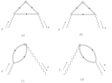
Figure 2: The diagrams for ${\widetilde{A}}_{n}^{H(1)}$. The double lines express the heavy quark.

IV The NLO PDFs in DIS_γ Scheme

The structure functions of the photon (nucleon) are expressed as convolutions of coefficient functions and parton distributions of the target photon (nucleon). But it is well known that these coefficient functions and parton distributions are by themselves factorization-scheme dependent. The relevant quantities given in Sec. III were calculated in $\rm{\overline{MS}}$ scheme. When we insert them into the formulae given by (26) and (27), we obtain the parton distributions predicted by $\rm{\overline{MS}}$ scheme. Meanwhile, an interesting and also useful factorization scheme called DIS_γ was introduced in the analysis of the photon structure function $F_{2}^{\gamma}$ GRV1992a . In this scheme, the photonic coefficient function $C_{2}^{\gamma}$, i.e., the direct photon contribution to $F_{2}^{\gamma}$, is absorbed into the photonic quark distributions.

The Mellin moments of the virtual photon structure function $\frac{1}{x}F_{2}^{\gamma}(x,Q^{2},P^{2})$ is expressed as

$$\int_{0}^{1}dxx^{n-1}\frac{1}{x}~{}F_{2}^{\gamma}(x,Q^{2},P^{2}) \equiv F_{2}^{\gamma}(n,Q^{2},P^{2})$$ (78)

$$= \bm{q}^{\gamma}(n,Q^{2},P^{2})\cdot\bm{C}_{2}(n,Q^{2})+C_{2}^{\gamma}(n,Q^{2})~{},$$

where $\bm{q}^{\gamma}(n,Q^{2},P^{2})$ is the four-component row vector given in (4). The column vector $\bm{C}_{2}(n,Q^{2})$ is made up of four hadronic coefficient functions,

$$\bm{C}_{2}(n,Q^{2}) \equiv (C_{2}^{Ls}(n,Q^{2}),~{}C_{2}^{H}(n,Q^{2}),~{}C_{2}^{G}(n,Q^{2}),~{}C_{2}^{Lns}(n,Q^{2}))^{\rm T},$$ (79)

where $C_{2}^{Ls},C_{2}^{H},C_{2}^{G}$ and $C_{2}^{Lns}$ are coefficient functions corresponding to the light “flavor-singlet” quark, heavy quark, gluon and light “flavor-nonsinglet” quark, respectively. The last term $C_{2}^{\gamma}(n,Q^{2})$ in (78) is the photonic coefficient function. The moments of the parton distributions in ${\rm DIS}_{\gamma}$ scheme are obtained as follows GRV1992a ; MVV2002 . In this scheme, the hadronic coefficient functions are the same as their counterparts in ${\overline{\rm MS}}$ scheme, but the photonic coefficient function is absorbed into the quark distributions and thus set to zero,

$${\bm{C}}_{2}(n,Q^{2})|_{{\rm DIS}_{\gamma}}={\bm{C}}_{2}(n,Q^{2})|_{\overline{\rm MS}}~{},\qquad C_{2}^{\gamma}(n,Q^{2})|_{{\rm DIS}_{\gamma}}=0.$$ (80)

Then Eq. (78) gives

$$F_{2}^{\gamma}(n,Q^{2},P^{2}) = \bm{q}^{\gamma}(n,Q^{2},P^{2})|_{{\rm DIS}_{\gamma}}\cdot\bm{C}_{2}(n,Q^{2})|_{{\rm DIS}_{\gamma}}$$ (81)

$$= \bm{q}^{\gamma}(n,Q^{2},P^{2})|_{{\rm DIS}_{\gamma}}\cdot\bm{C}_{2}(n,Q^{2})|_{\overline{\rm MS}}~{}.$$

On the other hand, $F_{2}^{\gamma}(n,Q^{2},P^{2})$ is expressed in ${\overline{\rm MS}}$ scheme as

$$F_{2}^{\gamma}(n,Q^{2},P^{2})=\bm{q}^{\gamma}(n,Q^{2},P^{2})|_{\overline{\rm MS}}\cdot\bm{C}_{2}(n,Q^{2})|_{\overline{\rm MS}}+C_{2}^{\gamma}(n,Q^{2})|_{\overline{\rm MS}}~{}.$$ (82)

We expand $\mbox{\boldmath$q$}^{\gamma}(n,Q^{2},P^{2})|_{{\rm DIS}_{\gamma}}$ in terms of the LO and NLO distributions and $\mbox{\boldmath$C$}_{2}(n,Q^{2})|_{\overline{\rm MS}}$ in powers of $\alpha_{s}(Q^{2})$ up to the NLO as follows:

$$\mbox{\boldmath$q$}^{\gamma}(n,Q^{2},P^{2})|_{{\rm DIS}_{\gamma}} = \mbox{\boldmath$q$}_{n}^{\gamma(0)}+\mbox{\boldmath$q$}_{n}^{\gamma(1)}|_{{\rm DIS}_{\gamma}}+\cdots~{},$$ (83)

$$\mbox{\boldmath$C$}_{2}(n,Q^{2})|_{\overline{\rm MS}} = \mbox{\boldmath$C$}_{2,n}^{(0)}+\frac{\alpha_{s}(Q^{2})}{4\pi}\mbox{\boldmath$C$}_{2,n}^{(1)}|_{\overline{\rm MS}}+\cdots~{},$$ (84)

where the LO $\mbox{\boldmath$q$}_{n}^{\gamma(0)}$ and $\mbox{\boldmath$C$}_{2,n}^{(0)}$ are both factorization-scheme independent. Denoting the difference of $\mbox{\boldmath$q$}_{n}^{\gamma(1)}|_{{\rm DIS}_{\gamma}}$ from ${\overline{\rm MS}}$ scheme prediction as $\delta{\mbox{\boldmath$q$}}_{n}^{\gamma(1)}|_{{\rm DIS}_{\gamma}}$, we write

$${\mbox{\boldmath$q$}}_{n}^{\gamma(1)}|_{{\rm DIS}_{\gamma}}\equiv{\mbox{\boldmath$q$}}_{n}^{\gamma(1)}|_{\overline{\rm MS}}+\delta{\mbox{\boldmath$q$}}_{n}^{\gamma(1)}|_{{\rm DIS}_{\gamma}}~{}.$$ (85)

Putting (83)-(85) into the r.h.s. of (81) and comparing the result with (82), we find

$$C_{2}^{\gamma}(n,Q^{2})|_{\overline{\rm MS}}=\delta\mbox{\boldmath$q$}_{n}^{\gamma(1)}|_{{\rm DIS}_{\gamma}}\cdot\mbox{\boldmath$C$}_{2,n}^{(0)}+\cdots~{}.$$ (86)

Since

$$\mbox{\boldmath$C$}_{2,n}^{(0)}=\left(\langle e^{2}\rangle_{L},e_{H}^{2},0,1\right)^{\rm T}~{},$$ (87)

the r.h.s. of Eq. (86) is rewritten as

$$\delta\mbox{\boldmath$q$}_{n}^{\gamma(1)}|_{{\rm DIS}_{\gamma}}\cdot\mbox{\boldmath$C$}_{2,n}^{(0)} = \langle e^{2}\rangle_{L}~{}\delta q_{Ls,n}^{\gamma(1)}|_{{\rm DIS}_{\gamma}}+e_{H}^{2}\delta q_{H,n}^{\gamma(1)}|_{{\rm DIS}_{\gamma}}+\delta q_{Lns,n}^{\gamma(1)}|_{{\rm DIS}_{\gamma}}~{}.$$ (88)

The moment of the photonic coefficient function $C_{2}^{\gamma}(n,Q^{2})|_{\overline{\rm MS}}$ is written up to the one-loop level as

$$C_{2}^{\gamma}(n,Q^{2})|_{\overline{\rm MS}}=\frac{\alpha}{4\pi}3\Bigl{\{}(n_{f}-1)\langle e^{4}\rangle_{L}B_{\gamma}^{L,n}+e_{H}^{4}B_{\gamma}^{H,n}\Bigr{\}}+\cdots~{}.$$ (89)

Now dividing the light quark-charge factor $\langle e^{4}\rangle_{L}$ into two parts, the light flavor-singlet and nonsinglet parts, as

$$\langle e^{4}\rangle_{L}=\langle e^{2}\rangle_{L}\langle e^{2}\rangle_{L}+\left(\langle e^{4}\rangle_{L}-(\langle e^{2}\rangle_{L})^{2}\right)~{},$$ (90)

and from Eqs. (88) and (89) we find at the NLO

$$\delta q^{\gamma(1)}_{Ls,n}|_{{\rm DIS}_{\gamma}} = \frac{\alpha}{4\pi}3(n_{f}-1)\langle e^{2}\rangle_{L}~{}B_{\gamma}^{L,n}~{},$$ (91)

$$\delta q^{\gamma(1)}_{H,n}|_{{\rm DIS}_{\gamma}} = \frac{\alpha}{4\pi}3~{}e_{H}^{2}~{}B_{\gamma}^{H,n}~{},$$ (92)

$$\delta q^{\gamma(1)}_{Lns,n}|_{{\rm DIS}_{\gamma}} = \frac{\alpha}{4\pi}3(n_{f}-1)\left(\langle e^{4}\rangle_{L}-(\langle e^{2}\rangle_{L})^{2}\right)B_{\gamma}^{L,n}~{}~{}.$$ (93)

The coefficient $B_{\gamma}^{L,n}$ is related to the one-loop gluon coefficient ${\overline{B}}_{G}^{n}$ by $B_{\gamma}^{L,n}=\frac{2}{n_{f}}{\overline{B}}_{G}^{n}$ BB , and given by

$$B_{\gamma}^{L,n}=4\left[-\frac{n^{2}+n+2}{n(n+1)(n+2)}\left(1+S_{1}(n)\right)+\frac{4}{(n+1)}-\frac{4}{(n+2)}+\frac{1}{n^{2}}\right],$$ (94)

while $B_{\gamma}^{H,n}$ is calculated in the heavy quark mass limit ($\Lambda^{2}\ll P^{2}\ll m^{2}$) and we find

$$B_{\gamma}^{H,n}=B_{\gamma}^{L,n}~{}.$$ (95)

Finally in ${\rm DIS}_{\gamma}$ scheme we set in all orders

$$G^{\gamma}(n,Q^{2},P^{2})|_{{\rm DIS}_{\gamma}}=G^{\gamma}(n,Q^{2},P^{2})|_{\overline{\rm MS}}~{}.$$ (96)

V Numerical analysis for PDFs with heavy quark effects

The parton distributions are recovered from their moments by the inverse Mellin transformation. Using the formulae given in Eqs. (26)-(31) and parameters enumerated in Sec. III, we obtain the parton distribution functions in the virtual photon in $\overline{\text{MS}}$ scheme up to the NLO . We have considered the following two cases:

1. $Q^{2}=5\text{GeV}^{2}$ and $P^{2}=0.35\text{GeV}^{2}$,

2. $Q^{2}=30\text{GeV}^{2}$ and $P^{2}=0.35\text{GeV}^{2}$.

In both cases we take $n_{f}=4$, and choose $c$ as a heavy quark and assume that the other $u$, $d$ and $s$-quarks are massless. We take $m_{c}=1.3\text{GeV}$ as an input for the charm quark mass and put $\Lambda=0.2\text{GeV}$ for the QCD scale parameter.

The values of $Q^{2}$ and $P^{2}$ for the case (i) correspond to those of the PLUTO experiment PLUTO . We plot the parton distribution functions in $\overline{\text{MS}}$ scheme in Fig. 3 for the case (i) and in Fig. 4 for the case (ii): (a) the light “flavor-singlet” quark distribution $xq^{\gamma}_{Ls}(x,Q^{2},P^{2})|_{\overline{\text{MS}}}$, (b) the heavy (charm) quark distribution $xq^{\gamma}_{H}(x,Q^{2},P^{2})|_{\overline{\text{MS}}}$, (c) the gluon distribution $xG^{\gamma}(x,Q^{2},P^{2})|_{\overline{\text{MS}}}$ and (d) the light “flavor-nonsinglet” quark distribution $xq^{\gamma}_{Lns}(x,Q^{2},P^{2})|_{\overline{\text{MS}}}$. In order to see the heavy quark effects, we plot, in addition, the parton distributions $xq^{\gamma}_{Ls}|_{\text{light},\overline{\text{MS}}}$, $xq^{\gamma}_{H}|_{\text{light},\overline{\text{MS}}}$ and $xG^{\gamma}|_{\text{light},\overline{\text{MS}}}$ which are obtained when $c$-quark is also set to be massless. Actually, we get these distributions by setting $\Delta{\widetilde{A}}^{n}_{H}\to 0$ in Eq. (74) and by inserting the “new” row vector ${\widetilde{\mbox{\boldmath$A$}}}_{n}^{(1)}$ into the expression of Eq. (27). See also Appendix A. Since the light “flavor-nonsinglet” quark decouples to the other partons, we have $xq^{\gamma}_{Lns}|_{\text{light}}=xq^{\gamma}_{Lns}$.

We observe from Fig. 3 (a)-(c) and Fig. 4 (a)-(c) that the $c$-quark mass has rather large effects on the $c$-quark distribution $xq^{\gamma}_{H}|_{\overline{\text{MS}}}$ and the gluon distribution $xG^{\gamma}|_{\overline{\text{MS}}}$, while it has negligible effects on the light “flavor-singlet” quark distribution $xq^{\gamma}_{Ls}|_{\overline{\text{MS}}}$. The difference between $xq^{\gamma}_{Ls}|_{\overline{\text{MS}}}$ and $xq^{\gamma}_{Ls}|_{\text{light},\overline{\text{MS}}}$ (and also between $xq^{\gamma}_{H}|_{\overline{\text{MS}}}$ and $xq^{\gamma}_{H}|_{\text{light},\overline{\text{MS}}}$ and between $xG^{\gamma}|_{\overline{\text{MS}}}$ and $xG^{\gamma}|_{\text{light},\overline{\text{MS}}}$) is due to the appearance of $\Delta{\widetilde{A}}^{n}_{H}$ in Eq. (74), which is negative and larger in magnitude for smaller $n$. The negative $\Delta{\widetilde{A}}^{n}_{H}$ means that once $c$-quark has mass, the $c$-partons are less produced from the target photon. Actually it has the same effect as reducing the evolution of $c$-quark distribution to the range of $m^{2}$ to $Q^{2}$ instead of $P^{2}$ to $Q^{2}$. Indeed we find from Eq. (27),

$$\left(q^{\gamma}_{Ls,n}-q^{\gamma}_{Ls,n}|_{\text{light}}\right)/\left(\frac{\alpha}{8\pi\beta_{0}}\right) = \left(1-\frac{1}{n_{f}}\right)2\beta_{0}\Delta{\widetilde{A}}^{n}_{H}\bigg{\{}-(r)^{d_{\psi}^{n}}+\frac{\gamma_{\psi\psi}^{(0),n}-\lambda_{-}^{n}}{\lambda_{+}^{n}-\lambda_{-}^{n}}(r)^{d_{+}^{n}}+\frac{\gamma_{\psi\psi}^{(0),n}-\lambda_{+}^{n}}{\lambda_{-}^{n}-\lambda_{+}^{n}}(r)^{d_{-}^{n}}\biggr{\}}~{},$$ (97)

$$\left(q^{\gamma}_{H,n}-q^{\gamma}_{H,n}|_{\text{light}}\right)/\left(\frac{\alpha}{8\pi\beta_{0}}\right) = 2\beta_{0}\Delta{\widetilde{A}}^{n}_{H}\biggl{\{}\left(1-\frac{1}{n_{f}}\right)(r)^{d_{\psi}^{n}}+\frac{1}{n_{f}}\frac{\gamma_{\psi\psi}^{(0),n}-\lambda_{-}^{n}}{\lambda_{+}^{n}-\lambda_{-}^{n}}(r)^{d_{+}^{n}}+\frac{1}{n_{f}}\frac{\gamma_{\psi\psi}^{(0),n}-\lambda_{+}^{n}}{\lambda_{-}^{n}-\lambda_{+}^{n}}(r)^{d_{-}^{n}}\biggr{\}}~{},$$

where $r=\frac{\alpha_{s}(Q^{2})}{\alpha_{s}(P^{2})}$. Unless $n$ is a small integer, we see $\gamma_{\psi\psi}^{(0),n}\approx\lambda_{-}^{n}$ and $d_{\psi}^{n}\approx d_{-}^{n}$. Therefore the sum in the curly brackets of Eq. (97) diminishes, which means that the effects of heavy quark on $xq^{\gamma}_{Ls}$ are extremely small. See Fig. 3 (a) and Fig. 4 (a). On the other hand, the sum in the curly brackets of Eq. (LABEL:DeltaqH) is expressed approximately as $(r)^{d_{\psi}^{n}}$ for $n$ not being a small integer. The ratio of $(q^{\gamma}_{H,n}-q^{\gamma}_{H,n}|_{\text{light}})$ to the leading order $q^{\gamma(0)}_{H,n}$ is proportional to the product of $\alpha_{s}(Q^{2})$ and $(r)^{d_{\psi}^{n}}$. The values of $r$ and $\alpha_{s}(Q^{2})$ are 0.463 and 0.237, respectively, for the case (i) and 0.351 and 0.180 for the case (ii). The ratio is not small and Fig. 3 (b) and Fig. 4 (b) show the large reduction of $xq^{\gamma}_{H}|_{\overline{\text{MS}}}$ from $xq^{\gamma}_{H}|_{\text{light},\overline{\text{MS}}}$, especially, for the case (i).

The gluons do not couple to the photon directly and they are produced from the target photon through quarks. Therefore, the leading contribution to the gluon distribution $xG^{\gamma}|_{\overline{\text{MS}}}$ is essentially of order $\alpha$ and it is very small in absolute value except in the small $x$ region. The $c$-quark mass effects appear in $xG^{\gamma}|_{\overline{\text{MS}}}$ in the NLO (the order $\alpha$) and are enhanced by the charge factor $e_{H}=2/3$ (see Figs. 3 (c) and 4 (c)). The departure of $xq^{\gamma}_{Ls}|_{\overline{\text{MS}}}$ from $xq^{\gamma}_{Ls}|_{\text{light},\overline{\text{MS}}}$ at small $x$ is related to the behaviors of the gluon distributions $xG^{\gamma}|_{\overline{\text{MS}}}$ and $xG^{\gamma}|_{\text{light},\overline{\text{MS}}}$. As $x\to 0$, the both gluon distributions grow while their difference becomes larger.

Figs. 3 (d) and 4 (d) show the light “flavor-nonsinglet” quark distribution $xq^{\gamma}_{Lns}|_{\overline{\text{MS}}}$. Comparing with the graphs of $xq^{\gamma}_{Ls}|_{\overline{\text{MS}}}$, it is very small in absolute value. This is due to the fact that $xq^{\gamma}_{Lns}|_{\overline{\text{MS}}}$ has the charge factor $(\langle e^{4}\rangle_{L}-(\langle e^{2}\rangle_{L})^{2})$ which is a very small number (2/81 for $n_{f}=4$). An examination of Fig. 3 (b), (c) and Fig. 4 (b), (c) show that with larger $Q^{2}$, the $c$-quark mass effects become smaller. When $Q^{2}$ gets still larger, we may need to consider the $b$-quark mass effects with taking $n_{f}=5$, but $b$-quark has milder effects than $c$-quark because of its charge factor.

We see from Fig. 3 (a), (b), (d) and Fig. 4 (a), (b), (d) that the quark distributions $xq^{\gamma}_{Ls}|_{\overline{\text{MS}}}$, $xq^{\gamma}_{H}|_{\overline{\text{MS}}}$ and $xq^{\gamma}_{Lns}|_{\overline{\text{MS}}}$ diverge as $x\rightarrow 1$. This is due to the NLO contributions to the quark parton distributions in ${\overline{\text{MS}}}$ scheme. The behaviors of parton distributions near $x=1$ are governed by the large-$n$ limit of those moments. In the leading order, parton distributions are factorization-scheme independent. For large $n$, the moments of the LO quark distributions, $q^{\gamma(0)}_{Ls}$, $q^{\gamma(0)}_{H}$ and $q^{\gamma(0)}_{Lns}$, behave as $1/(n\,\ln n)$. Thus, in $x$ space, these LO quark distributions vanish for $x\rightarrow 1$ as $[-1/\ln(1-x)]$. On the other hand, the moments of the NLO quark distributions in $\overline{\rm MS}$ scheme, $q^{\gamma(1)}_{Ls}|_{\overline{\rm MS}}$, $q^{\gamma(1)}_{H}|_{\overline{\rm MS}}$ and $q^{\gamma(1)}_{Lns}|_{\overline{\rm MS}}$, behave in large-$n$ limit as $(\ln n)/n$. Therefore, in $x$ space, the (LO+NLO) quark distributions in ${\overline{\rm MS}}$ scheme positively diverge as $[-\ln(1-x)]$ for $x\rightarrow 1$. The moments of the LO and NLO gluon distributions, $G_{n}^{\gamma(0)}$ and $G_{n}^{\gamma(1)}$, behave for large $n$ as $1/(n\,\ln n)^{2}$ and $1/n^{2}$, respectively, and thus, in $x$ space, the (LO + NLO) curve of the gluon distribution (both $G^{\gamma}|_{\overline{\text{MS}}}$ and $G^{\gamma}|_{\text{light},\overline{\text{MS}}}$) vanishes as $(-\ln x)$ for $x\rightarrow 1$.

In $\text{DIS}_{\gamma}$ scheme the photonic coefficient $C_{2}^{\gamma}$ is absorbed into the quark distributions. In consequence, the (LO+NLO) quark distributions show different behaviors at large $x$ from those in $\overline{\text{MS}}$ scheme. Since $B_{\gamma}^{L,n}(=B_{\gamma}^{H,n})$ in Eq. (89) behaves as $(-4\ln n)/n$ for large $n$, the (LO+NLO) curves in $x$ space for $q^{\gamma}_{Ls}|_{\text{DIS}_{\gamma}}$, $q^{\gamma}_{H}|_{\text{DIS}_{\gamma}}$ and $q^{\gamma}_{Lns}|_{\text{DIS}_{\gamma}}$ negatively diverge as $\ln(1-x)$ for $x\rightarrow 1$. In fact, using Eqs. (91)-(96) and inverting the moments, we obtain parton distributions in $\text{DIS}_{\gamma}$ scheme up to the NLO, which are plotted in Fig. 5 and Fig. 6. Again we have considered the two cases: (i) $Q^{2}=5\text{GeV}^{2}$, $P^{2}=0.35\text{GeV}^{2}$ and (ii) $Q^{2}=30\text{GeV}^{2}$, $P^{2}=0.35\text{GeV}^{2}$. The other parameters are the same as before and $c$-quark is taken to be heavy. We see from Fig. 5 (a), (b), (c) and Fig. 6 (a), (b), (c) that the quark distributions $xq^{\gamma}_{Ls}|_{\text{DIS}_{\gamma}}$, $xq^{\gamma}_{H}|_{\text{DIS}_{\gamma}}$ and $xq^{\gamma}_{Lns}|_{\text{DIS}_{\gamma}}$ become negative at large $x$. We observe again that the mass of $c$-quark has negligible effects on the light “flavor-singlet” quark distribution  $xq^{\gamma}_{Ls}|_{\text{DIS}_{\gamma}}$ but large effects on the $c$-quark distribution $xq^{\gamma}_{H}|_{\text{DIS}_{\gamma}}$. When $Q^{2}$ gets larger, the heavy quark mass effects become smaller. It is noted that if we take into account the charge factors, the following three “renormalized” distributions, $x{\widetilde{q}}^{\gamma}_{Ls}|_{\text{light},\text{DIS}_{\gamma}}\equiv xq^{\gamma}_{Ls}|_{\text{light},{\text{DIS}_{\gamma}}}/\langle e^{2}\rangle_{L}$, $x{\widetilde{q}}^{\gamma}_{H}|_{\text{light},{\text{DIS}_{\gamma}}}\equiv xq^{\gamma}_{H}|_{\text{light},\text{DIS}_{\gamma}}/e_{H}^{2}$ and $x{\widetilde{q}}^{\gamma}_{Lns}|_{\text{DIS}_{\gamma}}\equiv xq^{\gamma}_{Lns}|_{\text{DIS}_{\gamma}}/\left(\langle e^{4}\rangle_{L}-(\langle e^{2}\rangle_{L})^{2}\right)$ overlap for almost the whole $x$ region except near $x=0$ (see Fig. 5 (a), (b) and (c) and Fig. 6 (a), (b) and (c) ).

Finally the gluon distribution $xG^{\gamma}|_{\text{DIS}_{\gamma}}$ is the same as $xG^{\gamma}|_{\overline{\text{MS}}}$.

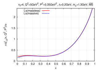
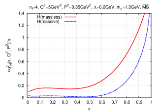
(a)	(b)
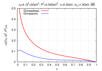
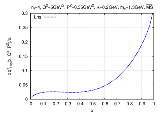
(c)	(d)

Figure 3: Parton distributions in the photon in $\overline{\rm MS}$ scheme for $n_{f}=4$, $Q^{2}=5$GeV², $P^{2}=0.35$GeV² with $m_{c}=1.3$GeV and $\Lambda=0.2$GeV: (a) $xq_{Ls}^{\gamma}(x,Q^{2},P^{2})|_{\overline{\rm MS}}$ and $xq_{Ls}^{\gamma}(x,Q^{2},P^{2})|_{\text{light,}\overline{\rm MS}}$; (b) $xq_{H}^{\gamma}(x,Q^{2},P^{2})|_{\overline{\rm MS}}$ and $xq_{H}^{\gamma}(x,Q^{2},P^{2})|_{\text{light,}\overline{\rm MS}}$; (c) $xG^{\gamma}(x,Q^{2},P^{2})|_{\overline{\rm MS}}$ and $xG^{\gamma}(x,Q^{2},P^{2})|_{\text{light,}\overline{\rm MS}}$; (d) $xq_{Lns}^{\gamma}(x,Q^{2},P^{2})|_{\overline{\rm MS}}$.

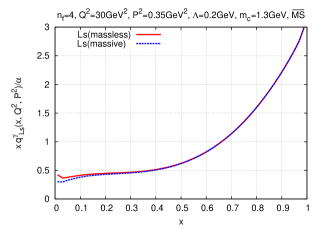
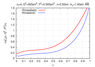
(a)	(b)
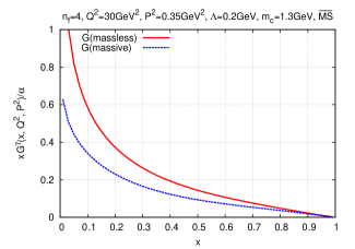
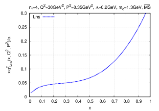
(c)	(d)

Figure 4: Parton distributions in the photon in $\overline{\rm MS}$ scheme for $Q^{2}=30$GeV². The other parameters are the same as in Fig. 3.

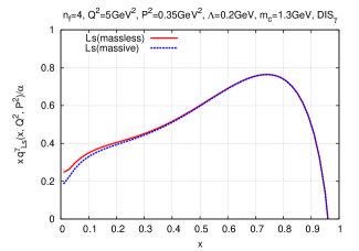
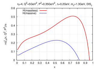
(a)	(b)
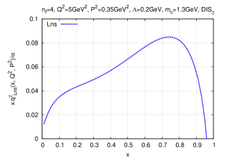
(c)

Figure 5: Parton distributions in the photon in DIS_γ scheme for $n_{f}=4$, $Q^{2}=5$GeV², $P^{2}=0.35$GeV² with $m_{c}=1.3$GeV and $\Lambda=0.2$GeV: (a) $xq_{Ls}^{\gamma}(x,Q^{2},P^{2})|_{\text{DIS}_{\gamma}}$ and $xq_{Ls}^{\gamma}(x,Q^{2},P^{2})|_{\text{light,DIS}_{\gamma}}$; (b) $xq_{H}^{\gamma}(x,Q^{2},P^{2})|_{\text{DIS}_{\gamma}}$ and $xq_{H}^{\gamma}(x,Q^{2},P^{2})|_{\text{light,DIS}_{\gamma}}$; (c) $xq_{Lns}^{\gamma}(x,Q^{2},P^{2})|_{\text{DIS}_{\gamma}}$.

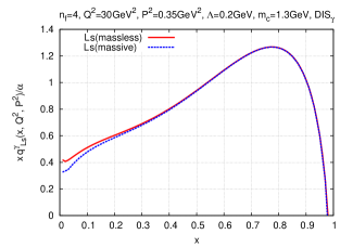
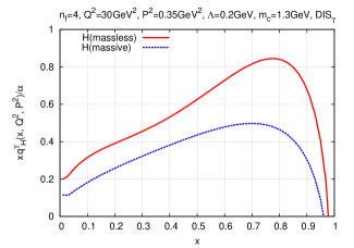
(a)	(b)
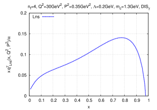
(c)

Figure 6: Parton distributions in the photon in DIS_γ scheme for $Q^{2}=30$GeV². The other parameters are the same as in Fig. 5.

VI Conclusions

We have studied the heavy quark mass effects on the parton (light singlet, heavy quark, gluon, light nonsinglet) distribution functions in the virtual photon up to the NLO in perturbative QCD. Our calculation is based on DGLAP equation as well as on the OPE formalism within the framework of the mass-independent renormalization group. The heavy quark effect is included through the operator matrix element for heavy quark operator and is evaluated by the heavy quark mass limit ($\Lambda^{2}\ll P^{2}\ll m^{2}$). In the language of the parton picture, the heavy quark effects are arising from the initial condition for the heavy quark distribution. In fact, the leading-logarithimic term of our initial condition (77) can be reproduced by solving the boundary condition, $q_{H}^{\gamma}(x,Q^{2}=m^{2})=0$ Fontannaz ; AFG , in the leading order approximation.

The heavy quark mass effects tend to reduce the values of parton distribution functions for the light-singlet, the heavy-quark and the gluon distributions except for the light nonsinglet distribution. Especially the suppression for the heavy parton distribution for the up-type quark is enhanced by the dependence of the charge factor $e_{i}=2/3$. These behaviors are consistent with our previous work on the virtual photon structure functions with the heavy quark mass effects KSUU2009 . These results could be explained by the suppression of the evolution range due to the mass of the heavy quark. We have also studied the factorization-scheme dependence of our parton distributions with heavy quark mass effects, especially for two factorization schemes, $\overline{\rm MS}$ and DIS_γ.

In our formalism where we treat the contribution from the twist-2 operators to the parton distributions, we have not taken into account the kinematical threshold effects which manifest as the presence of the maximal values of the Bjorken variable. We need some improvement in which the threshold effects are included. We should also investigate the general kinematical region where $P^{2}$ and $m^{2}$ are of the same order. We also note that the general-mass variable-flavor-number scheme (GM-VFNS), which has now become a popular framework for the global analyses of parton distributions, should be implemented in the present analysis which is under investigation.

Such improvements would help us to predict the photonic parton distribution functions which could be measured at the future linear collider ILC. Especially, the application of our results to the up-type quark parton distribution functions like the charm quark, the top quark in the unpolarized virtual photon will be important phenomenologically. The application of our formalism to the polarized photonic parton distribution functions can be carried out and would turn out to be relevant for the measurement of the polarized photonic PDFs at ILC.

Appendix A PDFs for the case of massless quarks

In this paper we have considered the parton distributions in the virtual photon for the case when the $n_{f}$-th flavor quark is heavy and the rest of $n_{f}-1$ flavor quarks are light (i.e., massless) and we have derived the formulae for the moments of the parton distributions, $q^{\gamma}_{Ls}(n,Q^{2},P^{2})$, $q^{\gamma}_{H}(n,Q^{2},P^{2})$, $G^{\gamma}(n,Q^{2},P^{2})$ and $q^{\gamma}_{Lns}(n,Q^{2},P^{2})$ up to NLO, which are given in Eqs. (28)-(31). If the $n_{f}$-th flavor quark is also light, in other words, all the $n_{f}$ flavor quarks are light, we obtain, instead, the parton distributions of $q^{\gamma}_{Ls}(n,Q^{2},P^{2})|_{\mbox{\scriptsize light}}$, $q^{\gamma}_{H}(n,Q^{2},P^{2})|_{\mbox{\scriptsize light}}$ and $G^{\gamma}(n,Q^{2},P^{2})|_{\mbox{\scriptsize light}}$ and $q^{\gamma}_{Lns}(n,Q^{2},P^{2})|_{\mbox{\scriptsize light}}$. Here it is noted that since the light “flavor nonsinglet” quark does not couple to the heavy flavor, we see $q^{\gamma}_{Lns}(n,Q^{2},P^{2})|_{\mbox{\scriptsize light}}=q^{\gamma}_{Lns}(n,Q^{2},P^{2})$. When all the flavor quarks are light, we usually treat the quark sector which consists of the flavor-singlet and nonsinglet combinations defined as follows:

$$q_{S}^{\gamma}\equiv\sum_{i=1}^{n_{f}}q^{i}~{},\qquad q^{\gamma}_{NS}\equiv\sum_{i=1}^{n_{f}}e^{2}_{i}\Bigl{(}q^{i}-\frac{q^{\gamma}_{S}}{n_{f}}\Bigr{)}.$$ (99)

Also we introduce the following quark-charge factors:

$$\langle e^{2}\rangle=\frac{1}{n_{f}}\sum_{i=1}^{n_{f}}e_{i}^{2}~{},\qquad\langle e^{4}\rangle=\frac{1}{n_{f}}\sum_{i=1}^{n_{f}}e_{i}^{4}~{}.$$ (100)

These parton distributions, $q_{S}^{\gamma}$, $q^{\gamma}_{NS}$ and $G^{\gamma}|_{\mbox{\scriptsize light}}$, have been investigated in Refs. GRV1992a ; MVV2002 ; USU2009 . The quark parton distributions $q^{\gamma}_{Ls}|_{\mbox{\scriptsize light}}$, $q^{\gamma}_{H}|_{\mbox{\scriptsize light}}$ and $q^{\gamma}_{Lns}$ are related to $q_{S}^{\gamma}$ and $q^{\gamma}_{NS}$. Indeed they are expressed in terms of $q_{S}^{\gamma}$ and $q^{\gamma}_{NS}$ as follows:

$$q^{\gamma}_{Ls}(n,Q^{2},P^{2})\big{|}_{\mbox{\scriptsize light}} = q^{\gamma}_{S}(n,Q^{2},P^{2})-q^{\gamma}_{H}(n,Q^{2},P^{2})\big{|}_{\mbox{\scriptsize light}},$$ (101)

$$q^{\gamma}_{H}(n,Q^{2},P^{2})\big{|}_{\mbox{\scriptsize light}} = \frac{1}{n_{f}}\left[q^{\gamma}_{S}(n,Q^{2},P^{2})+\frac{e_{H}^{2}-\langle e^{2}\rangle}{\langle e^{4}\rangle-\langle e^{2}\rangle^{2}}~{}q^{\gamma}_{NS}(n,Q^{2},P^{2})\right],$$ (102)

$$q^{\gamma}_{Lns}(n,Q^{2},P^{2}) = \frac{n_{f}-1}{n_{f}}\frac{\langle e^{4}\rangle_{L}-\langle e^{2}\rangle^{2}_{L}}{\langle e^{4}\rangle-\langle e^{2}\rangle^{2}}~{}q^{\gamma}_{NS}(n,Q^{2},P^{2}),$$ (103)

where the NLO expressions of $q^{\gamma}_{S}(n,Q^{2},P^{2})$ and $q^{\gamma}_{NS}(n,Q^{2},P^{2})$ are given in Eqs. (2.33), (2.35) and (2.37) of Ref. USU2009 . The transformation rule for $q^{\gamma}_{S}$ and $q^{\gamma}_{NS}$ from the $\rm{\overline{MS}}$ scheme to the ${\rm DIS}_{\gamma}$ scheme are given in Eqs. (3.33) and (3.34), respectively, of the same reference.

References

(1)
http://lhc.web.cern.ch/lhc.
(2)
http://www.linearcollider.org/cms.
(3)
T. F. Walsh,
Phys. Lett. 36 B, 121 (1971);
S. J. Brodsky, T. Kinoshita and H. Terazawa,
Phys. Rev. Lett. 27, 280 (1971).
(4)
M. Krawczyk, A. Zembrzuski and M. Staszel,
Phys. Rept. 345, 265 (2001);
R. Nisius,
Phys. Rept. 332, 165 (2000);
M. Klasen,
Rev. Mod. Phys. 74, 1221 (2002);
I. Schienbein,
Ann. Phys. 301, 128 (2002);
R. M. Godbole,
Nucl. Phys. Proc. Suppl. 126, 414 (2004).
(5)
T. F. Walsh and P. M. Zerwas,
Phys. Lett. 44 B, 195 (1973);
R. L. Kingsley,
Nucl. Phys. B 60, 45 (1973).
(6)
N. Christ, B. Hasslacher and A. H. Mueller,
Phys. Rev. D 6, 3543 (1972).
(7)
E. Witten,
Nucl. Phys. B 120, 189 (1977).
(8)
W. A. Bardeen and A. J. Buras,
Phys. Rev. D 20, 166 (1979);
21, 2041(E) (1980).
(9)
G. Altarelli,
Phys. Rep. 81, 1 (1982).
(10)
R. J. DeWitt, L. M. Jones, J. D. Sullivan, D. E. Willen and H. W. Wyld, Jr.,
Phys. Rev. D 19, 2046 (1979);
D 20, 1751(E) (1979).
(11)
M. Glück and E. Reya,
Phys. Rev. D 28, 2749 (1983).
(12)
S. Moch, J. A. M. Vermaseren and A. Vogt,
Nucl. Phys. B 621, 413 (2002).
(13)
A. Vogt, S. Moch and J. Vermaseren,
Acta. Phys. Polon. B 37, 683 (2004).
(14)
K. Sasaki,
Phys. Rev. D 22, 2143 (1980);
Prog. Theor. Phys. Suppl. 77, 197 (1983).
(15)
M. Stratmann and W. Vogelsang,
Phys. Lett. B 386, 370 (1996).
(16)
M. Glück, E. Reya and C. Sieg,
Phys. Lett. B 503, 285 (2001);
Eur. Phys. J. C 20, 271 (2001).
(17)
T. Uematsu and T. F. Walsh,
Phys. Lett. 101 B, 263 (1981).
(18)
T. Uematsu and T. F. Walsh,
Nucl. Phys. B 199, 93 (1982).
(19)
G. Rossi,
Phys. Rev. D 29, 852 (1984).
(20)
F. M. Borzumati and G. A. Schuler,
Z. Phys. C 58, 139 (1993).
(21)
J. Chýla,
Phys. Lett. B 488, 289 (2000).
(22)
S. Moch, J. A. M. Vermaseren and A. Vogt,
Nucl. Phys. B 688, 101 (2004).
(23)
A. Vogt, S. Moch and J. A. M. Vermaseren,
Nucl. Phys. B 691, 129 (2004).
(24)
T. Ueda, K. Sasaki and T. Uematsu,
Phys. Rev. D 75, 114009 (2007).
(25)
Y. Kitadono, K. Sasaki, T. Ueda and T. Uematsu,
Phys. Rev. D 77, 054019 (2008).
(26)
K. Sasaki and T. Uematsu,
Phys. Rev. D 59, 114011 (1999).
(27)
H. Baba, K. Sasaki and T. Uematsu,
Phys. Rev. D 65, 114018 (2002).
(28)
K. Sasaki, T. Ueda and T. Uematsu,
Phys. Rev. D 73, 094024 (2006).
(29)
M. Drees and R. M. Godbole,
Phys. Rev. D 50, 3124 (1994).
(30)
M. Glück, E. Reya and M. Stratmann,
Phys. Rev. D 51, 3220 (1995);
Phys. Rev. D 54, 5515 (1996).
(31)
M. Fontannaz,
Eur. Phys. J. C 38, 297 (2004).
(32)
K. Sasaki and T. Uematsu,
Phys. Lett. B 473, 309 (2000);
Eur. Phys. J. C 20, 283 (2001).
(33)
T. Ueda, K. Sasaki and T. Uematsu,
Eur. Phys. J. C 62, 467 (2009).
(34)
M. Glück, E. Reya and A. Vogt,
Phys. Rev. D 46, 1973 (1992).
(35)
P. Aurenche, M. Fontannaz and J. Ph. Guillet,
Z. Phys. C 64, 621 (1994);
Eur. Phys. J. C 44, 395 (2005).
(36)
M. Glück, E. Reya and I. Schienbein,
Phys. Rev. D 60, 054019 (1999);
D 62, 019902(E) (2000);
Phys. Rev. D 63, 074008 (2001).
(37)
K. Sasaki, J. Soffer and T. Uematsu,
Phys. Rev. D 66, 034014 (2002).
(38)
F. Cornet, P. Jankowski, M. Krawczyk and A. Lorca,
Phys. Rev. D 68, 014010 (2003).
(39)
F. Cornet, P. Jankowski and M. Krawczyk,
Phys. Rev. D 70, 093004 (2004).
(40)
Y. Kitadono, K. Sasaki, T. Ueda and T. Uematsu,
Prog. Theor. Phys. 121, 495 (2009).
(41)
M. Buza, Y. Matiounine, J. Smith, R. Migneron and W. L. van Neerven,
Nucl. Phys. B 472, 611 (1996).
(42)
W. A. Bardeen, A. J. Buras, D. W. Duke and T. Muta,
Phys. Rev. D 18, 3998 (1978).
(43)
M. Glück, E. Reya and A. Vogt,
Phys. Rev. D 45, 3986 (1992).
(44)
W. Furmanski and R. Petronzio,
Z. Phys. C 11, 293 (1982).
(45)
E. G. Floratos, D. A. Ross and C. T. Sachrajda,
Nucl. Phys. B 129, 66 (1977);
B 139, 545(E) (1978);
B 152, 493 (1979).
(46)
Ch. Berger et al. (PLUTO Collaboration),
Phys. Lett. B 142, 119 (1984).