Geometric phase of a moving three-level atom

Abstract

In this paper, we investigate the geometric phase of the field interacting with $\Xi$-type moving three-level atom. The results show that the atomic motion and the field-mode structure play important roles in the evolution of the system dynamics and geometric phase. We test this observation with experimentally accessible parameters and some new aspects are obtained.

I Introduction

In recent years much attention has been paid to the quantum phases such as the Pancharatnam phase which was introduced in 1956 by Pancharatnam P56 in his studies of interference effects of polarized light waves. The geometric phase which was realized, in 1984 B84 , is a generic feature of quantum mechanics and depends on the chosen path in the space spanned by all the likely quantum states for the system. Also, it has been shown that such matrix element in quantum physics was proposed in path integral approach to quantum mechanics saw22 . This approach studies the multitude of quantum trajectories which connect two points in the Hilbert space: $\psi(q^{j}(0))$ and $\psi(q^{j}(t))$, where $q^{j}$ are generalized quantum coordinates. The definition of phase change for partial cycles was obtained by Jordan J88 and ideas of Pancharatnam were used SB88 ; BM87 to show that for the appearance of Pancharatnam’s phase the system needs to be neither unitary nor cyclic WB90 ; WL88 , and may interpreted by quantum measurements. In this regard, one should noticed that the geometric phase is different from other phase effects in cavity quantum electrodynamics. For example tangent and cotangent states slo89 are connected with the phase of atomic population in two level system and the same phase effects are proposed in three-level system ors92 .

Presently the models of quantum computation in which a state is an operator of density matrix are developed T02 . It is shown EEHI00 that the geometric phase shift can be used for generation fault-tolerance phase shift gates in quantum computation. Many generalizations have been proposed to the original definition VM00 ; A03 ; AAO00 ; Law99 . The quantum phase, including the total phase as well as its dynamical and geometric parts, of Pancharatnam type are derived for a general spin system in a time-dependent magnetic field based on the quantum invariant theory wag95 . Another approach that provides a unified way to discuss geometric phases in both photon (massless) and other massive particle systems was developed by Lu in Ref. lu99 . Also, an expression for the Pancharatnam phase for the entangled state of a two-1evel atom interacting with a single mode in an ideal cavity with the atom undergoing a two-photon transition was studied Law99 . To bring the two-photon processes closer to the experimental realization, the effect of the dynamic Stark shift in the evolution of the Pancharatnam phase has been presented AAO00 . More recently, a method for analyzing the geometric phase for $N$ two-level system of superconducting charge qubits interacting with a microwave field is proposed aty09 and through a simple but universal system (two-level atom) a possibility to control the Pancharatnam phase of a quantum system on a much more sensitive scale than the population dynamics has been reported bou09 . In Ref. P03 experiments are proposed for the observation of the nonlinearity of the Pancharatnam phase with a Michelson interferometer.

In this paper we extend these investigations to study the dynamics of a moving three-level atom interacting with a coherent field. An exact solution of a three-level atom in interaction with cavity field has been obtained chu82 and developed for arbitrary configuration of the levels li87 . We investigate the effect of different parameters of the system on the geometric phase. This paper is arranged as follows: In Sec. 2, we introduce the model and its solution by using the unitary transformations method. In Sec. 3, we investigate the geometric phase and the dynamical properties for different regimes. Numerical results for the geometric phase are discussed in Sec. 4. Finally conclusions are presented.

II The system

In this section, we discuss the model of a moving three-level atom with energy levels denoted by $|1\rangle,|2\rangle$ and $|3\rangle,$ where $|3\rangle$ is the ground level, $|2\rangle$ is the middle level and $|1\rangle$ is the upper level. The interaction Hamiltonian of the system in the rotating-wave approximation can written as yoo85

$$H_{I}=g\lambda(t)\left(a\sigma_{23}e^{i\Delta t}+a\sigma_{12}e^{-i\Delta t}+h.c.\frac{{}}{{}}\right),$$ (1)

where $a(a^{\dagger})$ are the annihilation (creation) operator of the field mode, $\sigma_{ij}=|i\rangle\langle j|$ are the atomic operators, $\Delta$ is the detuning of the field mode from the atomic middle level 2 $(\Delta=\omega-(\omega_{2}-\omega_{1})=\omega-(\omega_{2}-\omega_{3}))$ and $g$ is the atom–field coupling constant. We deal with the one-dimensional case of atomic motion along the cavity axis and denote by $\lambda(t)$ the shape function of the cavity field mode sar74 ; li87 ; ena08 ; sch89 . A realization of particular interest in which the atomic center-of-mass motion is classical can be written as $\lambda(t)=\sin(p\pi\upsilon t/L),$ where $\upsilon$ denotes the atomic motion velocity, $p$ stands for the number of half wavelengths of the mode in the cavity and $L$ is the cavity length in $z-$direction. The classical consideration of the atomic center-of-mass motion is very well obeyed under the ordinary experimental conditions eng94 . However under extreme circumstances the quantum nature of the center-of-mass motion may become important eng91 ; har91 . In Ref. eng94 it has been mentioned that in the time dependent evolution the integral of $\lambda(t)$ must be approximate with $\overline{\lambda}t$, where $\overline{\lambda}$ describes the mean value of the interaction constant between the atom and cavity mode.

In this paper we assume that, the initial state is given by $|\psi(0)\rangle$ $=|\psi_{A}(0)\rangle\otimes|\psi_{F}(0)\rangle,$ where $|\psi_{A}(0)\rangle$ is the initial state of the atom and $|\psi_{F}(0)\rangle$ is the initial state of the field. The combined atom-field system can be written as rei09

$$|\psi(0)\rangle=\sum_{l=0,1}\cos\left(\theta+\frac{l\pi}{2}\right)\left(\sum_{n=-l}^{\infty}\frac{q_{n+l}(1+r(-1)^{n+l})}{\sqrt{B}}|n+l\text{ }\rangle_{F}\right)|3-l\text{ }\rangle_{A},$$ (2)

where $B=(1+r^{2}+re^{-2n})$, $r$ is an arbitrary constant. In this case, $r=0,1,$ and $-1,$ corresponds to coherent state, even coherent and odd coherent state, respectively. While $q_{n}$ is the number-state expansion coefficient, $q_{n}=\langle n|\psi_{F}(0)\rangle,$ for coherent state $q_{n}=e^{-\bar{n}/2}\alpha^{n}/\sqrt{n!},$ and $\bar{n}=|\alpha|^{2}$ is the average photon number of the field.

III Geometric phase

For the quantum system evolving from an initial wavefunction to a final wavefunction, if the final wavefunction cannot be obtained from the initial wavefunction by a multiplication with a complex number, the initial and final states are distinct and the evolution is noncyclic. Suppose state $\left|\psi(0)\right\rangle$ evolves to a state $\left|\psi(t)\right\rangle$ after a certain time $t$. If the scalar product aha00

$$\left\langle\psi(0)\right|\exp\left[\frac{i}{\hbar}\int_{0}^{t}H(t^{\prime})dt^{\prime}\right]\left|\psi(0)\right\rangle,$$ (3)

can be written as $\Gamma\exp(i\gamma),$ where $\Gamma$ is a real number, then the noncyclic phase due to the evolution from $\left|\psi(0)\right\rangle$ to $\left|\psi(t)\right\rangle$ is the angle $\gamma.$ This noncyclic phase generalizes the cyclic geometric phase since the latter can be regarded as a special case of the former in which $\Gamma=1$. Determination of the phase between the two states for such an evolution is nontrivial. Pancharatnam prescribed the phase acquired during an arbitrary evolution of a wavefunction from the vector $\left|\psi(0)\right\rangle$ to $\left|\psi(t)\right\rangle$ as

$$\phi_{g}=\mathrm{arg}\left\langle\psi(0)\right|\left.\psi(t)\right\rangle.$$ (4)

Subtracting the dynamical phase from the Pancharatnam phase, we obtain the geometric phase. Here, for the time-dependent interaction and considering the resonant case, an exact expression of the geometric phase can be obtained as

$$\phi_{g}(t)=-\sin^{-1}\left\{\frac{y(t)}{\sqrt{x^{2}(t)+y^{2}(t)}}\right\},$$ (5)

where

$$x(t) = \sum_{n=0}^{\infty}\frac{q_{n}^{2}\cos^{2}\theta}{B(2n+3)}[1+r(-1)^{n}]^{2}[n+2+(n+1)\cos(\lambda_{1}(t)\sqrt{2n+3})]$$ (6)

$$+\sum_{n=0}^{\infty}\frac{q_{n+1}^{2}\sin^{2}\theta}{B}[1-r(-1)^{n}]^{2}\cos\left[\lambda_{1}(t)\sqrt{2n+3}\right],$$

$$y(t) = \sum_{n=0}^{\infty}\frac{q_{n}q_{n+1}\sin 2\theta}{B}\sqrt{\frac{n+1}{2n+3}}[1-r^{2}]\sin\left[\lambda_{1}(t)\sqrt{2n+3}\right],$$ (7)

$$\lambda_{1}(t) = \frac{L}{p\pi\upsilon}(1-\cos\left(p\pi\upsilon t/L\right)).\$$

More specifically, if we consider the atomic motion velocity as $\upsilon=gL/\pi$, then $\lambda_{1}(t)=\frac{1}{pg}(1-\cos\left(pgt\right)),\$while $\ \lambda_{1}(t)=gt,$ if the atomic motion is neglected.

For the off-resonant case, the numerical results will be used. In the time-independent case, characterized by the transformation matrix $\hat{U}(t),$ the geometric phase is defined through $|\psi(t)\rangle=\hat{U}(t)|\psi(0)\rangle$ and $\hat{U}(t)$ is given by

$$\hat{U}(t)=\sum_{j=1}^{3}\exp\left(-iE_{j}t\right)|\varphi_{j}\left(t\right)\rangle\langle\varphi_{j}\left(t\right)|,$$ (8)

where $|\varphi_{j}\left(t\right)\rangle$ and $E_{j\text{ }}\left(t\right)$ are eigenvectors and corresponding eigenvalues of the Hamiltonian $H_{I}.$

III.1 Numerical results

It is of rather more use to exhibit the numerical results explicitly for particular initial conditions of relevance to the experiments. With this in mind we will assume that the initial state is prepared according to Eq. (2) to be a particular coherent state, even coherent or odd coherent state, with the atom prepared in a superposition state. In the experiments done so far, it is possible to probe directly which electronic state the atom occupies. It was reported that bru96 the cavity can have a photon storage time of $T=1$ ms (corresponding to $Q=3\times 10^{8}$ ). The radiative time of the Rydberg atoms with the principle quantum numbers $49$, $50$ and $51$ is about $2\times 10^{-4}s$. In order to realize such a scheme in laboratory experiment within a microwave region, we may consider slow $Rb$ atoms in higher Rydberg states which have life time of the order of few milliseconds dav94 . The interaction times of atom with the cavity modes come out to be of the order of few tens of microseconds which is far less than the cavity life time. The high-Q cavities of life time of the order of millisecond are being used in experiments rau which opened interesting perspectives for quantum information manipulation and fundamental tests of quantum theory.

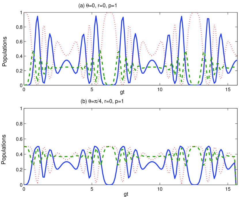
Figure 1: Time evolution of the populations $\rho_{11}$ (solid line), $\rho_{22}$ (dashed line), $\rho_{33}$ (dotted line) for $\alpha=5$, $\Delta=0$, $r=0,p=1$ and different values of $\theta,$ where (a) $\theta=0$ and (b) $\theta=\pi/4$.

It is clear that the geometric phase has zero value when $\theta=0$, this means physically that there is no phase in photon transition that make the photon transition is in a straight line and populations have values of oscillations between $0$ and $1.$ As a result of the numerical calculations, the oscillations will dephase and next will collapse after some times $t$ . In figure 1, we present a plot in which a comparison between the general behavior of atomic dynamic when $\theta=0$ and $\theta=\pi/4$ is presented. It is shown that for $\theta=0,$ the oscillations of the probability amplitudes are repeated periodically, the oscillations have peaks and bottoms where populations are vanished every time periodically at $t=\frac{2\pi}{p},p=1$. On the other hand, when $\theta=\pi/4,$ we observe that the amplitude of the oscillations is decreased and the maximum value of the populations does not exceed $0.5$.

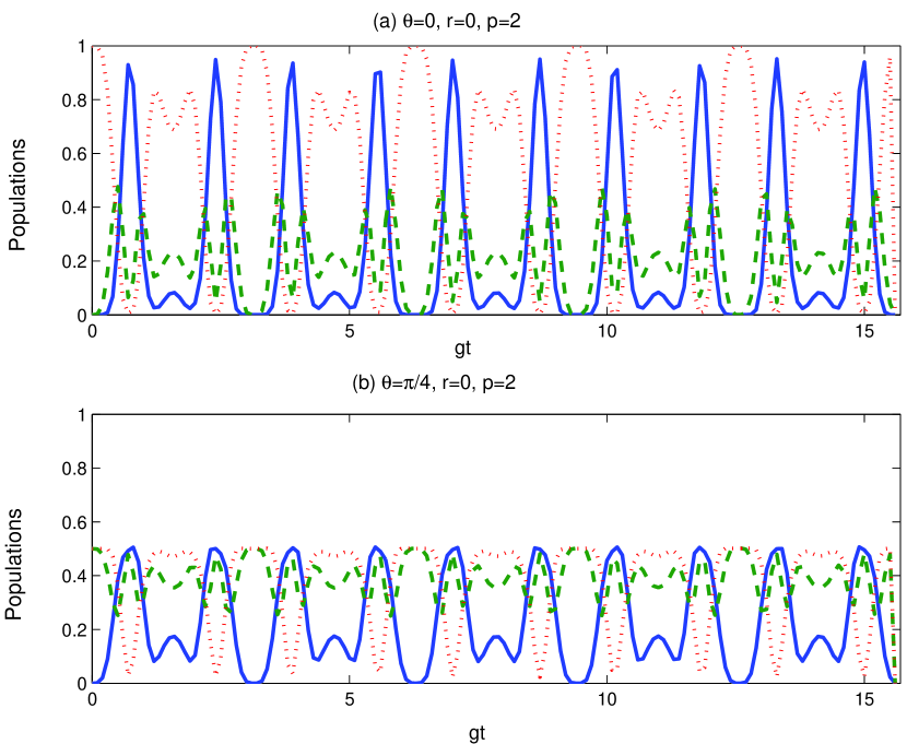
Figure 2: The same as figure 1 but $p=2.$

In figure 2 we compare the populations when $\theta=0$ and with that when $\theta=\pi/4$ in the same period of time (see figure 1). For $\theta=0,$ we still have the periodicity of the dynamics but in this case the vanishing time of the populations is given by $t=\frac{2\pi}{p},\left(p=2\right)$. Similar to the previous case for $\theta=\pi/4,$ the amplitude of the oscillations is decreased and the maximum value of the populations does not exceed $0.6$.

In Fig. 3a we have plotted the geometric phase $\phi_{t}$ as a function of the scaled time, $gt,$ where $r=0$ and $p=1.$ When $\theta=0$ we find that the geometric phase is vanished but for $\theta=\pi/4$ the geometric phase shows similar behavior to the periodic collapse-revival phenomenon of Rabi oscillation but with a period of ($t=\frac{2\pi}{p},p=1$). In Fig. 3b we have plotted the geometric phase, $\phi_{t\text{ }},$ as a function of the scaled time, $gt,$  where $r=0$ and $p=2.$ In this case, it is shown that the geometric phase has the same behavior of Fig. 3a but with a period of ($t=\frac{2\pi}{p},p=2$). In the off-resonant case, the geometric phase shows oscillatory behavior only during the first stage of the interaction (say $0\leq\lambda t\leq 10),$ followed by zero phase.

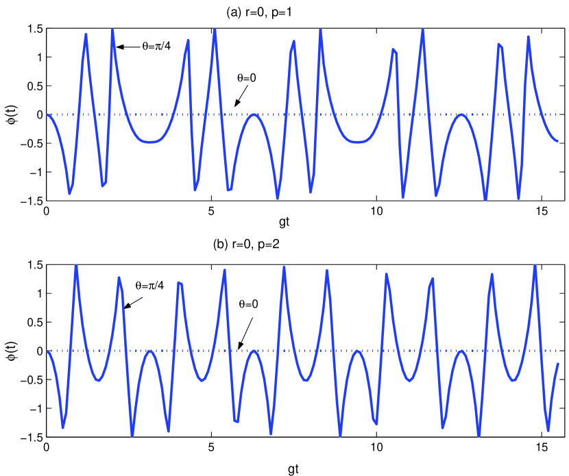
Figure 3: The geometric phase, $\phi\left(t\right),$ as a function of the scaled time $gt$. The other parameters are $\alpha=5$, $\Delta=0,$ $r=0$ and different values of $p$ and $\theta$ where (a) $p=1$ and (b) $p=2$ with $\theta=0$ (dotted curve) and $\theta=\pi/4$ (solid curve)

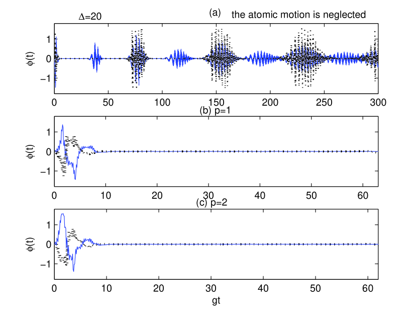
Figure 4: Time evolution of the geometric phase $\phi\left(t\right)$ for $\alpha=5$, $\Delta=20$, $\theta=\pi/4$ where (a) the atomic motion is neglected, (b) $p=1$, (c) $p=2$ with $r=1$ (dotted line) and $r=0$ (solid line).

In Fig. 4, we have plotted the geometric phase when we consider the influence of the detuning, $\Delta=20,$ and for different values of the parameter $r$ , where $r=0$ (solid line) and $r=1$ (dotted line ). In Fig. 4a the atomic motion is neglected $p=0.$ It is important to note that the geometric phase has a collapse-revival but the amplitude of the oscillations as well as the revival time become smaller and we have more revivals at the same period of time time and the two values of revival geometric phase which are corresponding to $r=0$ and $r=1$ repeating with the time development. In Fig. 4b, we consider $p=1$, keeping the same value of the parameter $r=1$ as in Fig. 4a. It is shown that the geometric phase has oscillations only at the initial stage of the interaction time.  As time goes on ($gt>8$), a disappearance of the geometric phase is observed and there is no more dependence on the interaction time.

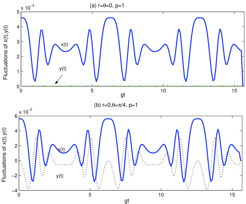
Figure 5: Time evolution of $x(t)$ (soled curve) and $y(t)$ (dotted curve), where $\langle\psi(0)|\psi(t)\rangle=x(t)+iy(t).$ The parameters are $\alpha=5$, $\Delta=0,$ $r=0,p=1$ and different values $\theta$ where (a) $\theta=0$ and (b) $\theta=\pi/4.$

It is rather interesting to mention to the fact that: in the Feynman approach to quantum mechanics it is important not only the modulus and argument of complex number, but the quantum fluctuations of this variables too. In such a representation, the deviation of quantum trajectories from the classical trajectories are described by the quantum fluctuations elu09 . Therefore we have further investigated the fluctuations of the real and imaginary parts of $\left\langle\psi(0)\right|\left.\psi(t)\right\rangle=x(t)+iy(t)$ for two different values of $\theta,$ where $\theta=0$ or $\theta=\pi/4$ (see Fig. 5). Fig. 5a gives a clear physical picture in this case for the disappearance of the geometric phase when $\theta=0,$ since $x(t)$ shows oscillations only while $y(t)=0$ everywhere. However, if the influence of the geometric phase on the parameter $\theta$ is to be included, e.g., $\theta=\pi/4$ (see Fig. 5b), oscillations are clearly observed for both $x(t)$ and $y(t)$ and hence the geometric phase exists in this case (see Fig. 3).

IV conclusion

In this paper we have investigated the quantum dynamics and geometric phase of the interaction between a moving three-level atom and a coherent field. We have used the unitary transformation method to obtain an exact expression of the geometric phase and numerical treatment has been used for the off-resonant case. The results point to a number of interesting features, which arise from the variation of the parameters of the system, namely, the atomic motion, and atomic superposition parameter. This result comes down to say that every parameter has an effect on the geometric phase. If the atom starts from an upper state, we find that there is no value of the geometric phase which means physically that the photon transition will occurs without any phase. Meanwhile, if the atom starts from a superposition case, the geometric phase will oscillates periodically depending on the value of atomic motion parameter $p.$

Acknowledgement

The authors would like to thank the referees for their objective comments that improved the text in many points.

References

- (1) S. Pancharatnam, Proc. Indian Acad. Sci. A 44, 247 (1956).
- (2) M.V. Berry, Proc. R. Soc. London Ser. A 392, 45 (1984).
- (3) M. S. Swanson, ”Path Integrals and Quantum Processes” (section 2.2, Academic Press Boston-San Diego-New York, 1992)
- (4) T.F. Jordan, Phys. Rev. A 38,1590 (1988).
- (5) J. Samuel, R. Bhandari, Phys. Rev. Lett. 60, 2339 (1988).
- (6) M.V. Berry, J.Mod. Opt. 34, 1401 (1987).
- (7) H. Weinfurter, G.Banudrek, Phys. Rev. Lett. 64, 1318 (1990).
- (8) Y.-S. Wu, H.-Z. Li, Phys. Rev. B 38, 11907 (1988).
- (9) J. J. Slosser and P. Meystre, Phys. Rev. Lett. 63, 934 (1989).
- (10) M. Orszag, J. C. Retamal and C. Saavedra, Phys. Rev. A 45, 2118 (1992); G. S. Agarwal, Phys. Rev. Lett. 71, 1351 (1993); N. A. Enakiand and N.Ciobanu, Opt. Comm. 282, 1825 (2009).
- (11) V.E. Tarasov, J. Phys. A 35, 5207 (2002).
- (12) E. Sjöqvist, A. K. Pati, A. K. Ekert, J. S. Anandan, M. Ericsson, D. K. L. Oi and V. Vedral, Phys. Rev. Lett. 85, 2845 (2000).
- (13) A. K. Ekert, M. Ericsson, P. Hayden, H. Inamori, J. A. Jones, D. K. L. Oi, and V. Vedral, J. Mod. Opt. 47, 2501 (2000).
- (14) M. Abdel-Aty, J. Opt. B 5, 349 (2003).
- (15) M. Abdel-Aty, S. Abdel-Khalek, A.-S.F. Obada, Opt. Rev. 7, 499 (2000).
- (16) Q. V. Lawande, S.V. Lawande, A. Joshi, Phys. Lett. A. 251, 164 (1999).
- (17) G. Wagh and V. C. Rakhecha: Phys. Lett. A Phys. Lett. A 197, I12 (1995).
- (18) J. Lu: Eur. Phys. J. D 5, 307 (1999).
- (19) M. Abdel-Aty, Phys. Lett. A 373, 3572 (2009).
- (20) M. A. Bouchene and M. Abdel-Aty, Phys. Rev. A 79, 055402 (2009).
- (21) A. Pati, Int. J. Quant. Inf. 1, 135 (2003).
- (22) S.-Y. Chu and D.-C. Su, Phys. Rev. A 25, 3169 (1982); N. N. Bogolubov, Jr., F. L. Kien and A. S. Shumovsky, Phys. Lett. 101A, 201 (1984); M. Abdel-Aty, A. McGurn, Phys. Lett. A 373, 2420 (2009).
- (23) X-S. Li, D. L. Lin, and C.-D. Gong, Phys. Rev. A 36, 5209 (1987).
- (24) H.-I. Yoo and J. H. Eberly, Phys. Rep. 118, 239 (1985); R. R. Puri, J. Mod. Opt. 46, 1465 (1999).
- (25) M. Sargent III, M.O. Scully, and W.E. Lamb, Jr., Laser physics (Addison-Wesley, Reading/Mass., 1974).
- (26) N. A. Enaki and N. Ciobanu J. Mod. Opt. 55, 1557 (2008).
- (27) R. R. Schlicher, Opt. Commun. 70, 97 (1989).
- (28) B.-G. Englert, quant-ph/0203052 (1994); H. J. Carmichael and B. C. Sanders, Phys. Rev. A 60, 2497 (1999); C. J. Hood, M. S. Chapman, T. W. Lynn, and H. J. Kimble , Phys. Rev. Lett. 80, 4157 (1998).
- (29) B.-G. Englert, J. Schwinger, A. O. Barut and M. O. Scully, Europhys. Lett. 14, 25 (1991).
- (30) W. P. Reinhardt, C. A. Stanich and C. D. Schillaci, Appl. Math. Inf. Sci. 3, 273 (2009).
- (31) S. Haroche, M. Brune and J. M. Raimond, Europhys. Lett. 14, 19 (1991).
- (32) Y. Aharonov and J. S. Anandan, Phys. Rev. Lett. 58, 1593 (1987); E. Sjöqvist, A. K. Pati, A. Ekert, J. S. Anandan, M. Ericsson, D. K. L. Oi, and V. Vedral, Phys. Rev. Lett. 85, 2845 (2000).
- (33) Ö. E. Müstecaphoğlu, Phys. Rev. A 68, 023811 (2003).
- (34) M. Brune, E. Hagley, J. Dreyer, X. Maitre, A. Maali, C. Wunderlich, J. M. Raimond and S. Haroche, Phys. Rev. Lett. 77, 4887 (1996).
- (35) L. Davidovich, N. Zagury, M. Brune, J. M. Raimond and S. Haroche, Phys. Rev. A 50, R895 (1994).
- (36) A. Rauschenbeutel, P. Bertet, S. Osnaghi, G. Nogues, M. Brune, J. M. Raimond and S. Haroche, Phys. Rev. A 64, 050301 (2001).
- (37) H. Eleuch, Appl. Math. Inf. Sci. 3, 185 (2009).