Y-system, TBA and Quasi-Classical Strings in $AdS_{4}\times{\mathbb{C}\mathbb{P}}^{3}$

Nikolay Gromov
Mathematics Department, King’s College London,
The Strand, London WC2R 2LS, UK &
DESY Theory, Notkestr. 85 22603 Hamburg, Germany &
II. Institut für Theoretische Physik Universität Hamburg, Luruper Chaussee 149 22761 Hamburg Germany &
St.Petersburg INP, Gatchina, 188 300, St.Petersburg, Russia
E-mail
nikgromov$∙$gmail.com
   Fedor Levkovich-Maslyuk
Physics Department, Moscow State University, 119991, Moscow, Russia
E-mail
fedor.levkovich$∙$gmail.com
Abstract:

We study the exact spectrum of the ${\rm AdS}_{4}/{\rm CFT}_{3}$ duality put forward by Aharony, Bergman, Jafferis and Maldacena (ABJM). We derive thermodynamic Bethe ansatz (TBA) equations for the planar ABJM theory, starting from “mirror” asymptotic Bethe equations which we conjecture. We also propose generalization of the TBA equations for excited states. The recently proposed Y-system is completely consistent with the TBA equations for a large subsector of the theory, but should be modified in general. We find the general asymptotic infinite length solution of the Y-system, and also several solutions to all wrapping orders in the strong coupling scaling limit. To make a comparison with results obtained from string theory, we assume that the all-loop Bethe ansatz of N.G. and P. Vieira is the valid worldsheet theory description in the asymptotic regime. In this case we find complete agreement, to all orders in wrappings, between the solution of our Y-system and generic quasi-classical string spectrum in ${\rm AdS}_{3}\times{\rm S}^{1}$.

AdS/CFT, Integrability

1 Introduction

The AdS/CFT correspondence [1] continues to be a source of exciting new results in gauge and string theories. The best-studied example of the duality is the correspondence between four-dimensional ${\cal N}=4$ super Yang-Mills (SYM) theory and Type IIB superstring theory on ${\rm AdS}_{5}\times{\rm S}^{5}$. Another example is the recently found duality between Type IIA string theory on ${\rm AdS}_{4}\times{\mathbb{CP}}^{3}$ and three-dimensional ${\cal N}=6$ super Chern-Simons (SCS) theory [2].

Remarkably, evidence for integrability has been found both in the gauge theory [3, 4] and in the string theory [5, 6] in the planar limit of large number of colors. In SYM further intensive development [7, 8] has led to complete description of anomalous dimensions of infinitely long operators by means of the Asymptotic Bethe Ansatz (ABA) equations [9, 10]. Similar equations were found in [12, 13] for SCS. Very recently the integrability approach was also extended to ${\rm AdS}_{3}/{\rm CFT}_{2}$ dual pairs [14].

For complete solution of the planar AdS/CFT spectral problem one should be able to solve the integrable two dimensional worldsheet theory in finite volume. The program of applying the methods of relativistic integrable field theories for finite size spectrum of AdS/CFT was started in [15]. In [16] a generalization of the Lüscher type formula was proposed for the first finite volume correction to the asymptotic spectrum generated by ABA. This information, as well as experience with relativistic integrable theories [18], led to the Y-system proposed in [19] for exact solution of both ${\rm AdS}_{5}\times{\rm S}^{5}$ and ${\rm AdS}_{4}\times{\mathbb{CP}^{3}}$ theories. As we show in this work, the proposal of [19] for ABJM theory is only valid in a certain large subsector of the theory, and should be modified to describe the general case.

Refer to caption Refer to caption
${{\rm AdS}_{5}\times{\rm S}^{5}}$ ${{\rm AdS}_{4}\times{\mathbb{CP}}^{3}}$
Figure 1: Graphical representation of the Y-systems [19]. Circles correspond to Y-functions. Black nodes are the “massive” nodes which are suppressed for asymptotically large length $L$. For gray circles in the corners the equation cannot be written “locally” in terms of Y’s.

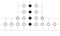
A graphical representation of the Y-systems of [19] is given in Fig. 1 where the Y-functions are represented by circles. Each value of the index $A$, which labels the Y-functions (functions of the spectral parameter $u$), corresponds to a node of this diagram. For each node $A$, except the gray ones, the Y-system equation has the form

$$Y_{A}^{+}Y_{A}^{-}=\frac{\prod_{B}(1+Y_{B})}{\prod_{C}(1+1/Y_{C})},$$ (1.1)

where $Y_{A}^{\pm}=Y_{A}(u\pm i/2)$ and the index $B$ (resp. $C$) labels the nodes connected to the $A$ node by horizontal (resp. vertical) lines.111For the gray node the equations cannot be written as functional equations in terms of $Y$’s. In many cases it is convenient to parameterize the Y-functions in terms of T-functions, which satisfy the Hirota functional equation. The “non-local” equation for the gray nodes is replaced (see for example [19]) by a “local” one in terms of T-functions.

In this paper we argue that in the AdS4/CFT3 case equation (1.1) for black nodes (Fig. 1, on the right) should be replaced by rather unusual equations

Ya+Yasuperscriptsubscript𝑌subscript𝑎superscriptsubscript𝑌subscript𝑎\displaystyle Y_{{\scalebox{0.67}{\begin{picture}(5.21,0.0)\put(-1.5,1.2){$\blacktriangleright$}\end{picture}}}_{a}}^{+}Y_{{\scalebox{0.67}{\begin{picture}(5.21,0.0)\put(-1.5,1.2){$\blacktriangleleft$}\end{picture}}}_{a}}^{-} =\displaystyle= 1+Ya(1+1/Ya+1)(1+1/Ya1),a>1,1subscript𝑌subscript𝑎11subscript𝑌subscript𝑎111subscript𝑌subscript𝑎1𝑎1\displaystyle\frac{1+Y_{\scalebox{0.6}[0.7]{\begin{picture}(7.24,0.2)\put(-1.5,0.5){$\bigtriangleup$}\end{picture}}_{a}}}{(1+1/Y_{\scalebox{0.67}{\begin{picture}(5.21,0.0)\put(-1.5,1.2){$\blacktriangleleft$}\end{picture}}_{a+1}})(1+1/Y_{\scalebox{0.67}{\begin{picture}(5.21,0.0)\put(-1.5,1.2){$\blacktriangleright$}\end{picture}}_{a-1}})}\,\,,\,\,a>1, (1.2)
Ya+Yasuperscriptsubscript𝑌subscript𝑎superscriptsubscript𝑌subscript𝑎\displaystyle{Y_{{\scalebox{0.67}{\begin{picture}(5.21,0.0)\put(-1.5,1.2){$\blacktriangleleft$}\end{picture}}}_{a}}^{+}Y_{{\scalebox{0.67}{\begin{picture}(5.21,0.0)\put(-1.5,1.2){$\blacktriangleright$}\end{picture}}}_{a}}^{-}} =\displaystyle= 1+Ya(1+1/Ya+1)(1+1/Ya1),a>1,1subscript𝑌subscript𝑎11subscript𝑌subscript𝑎111subscript𝑌subscript𝑎1𝑎1\displaystyle\frac{1+Y_{\scalebox{0.6}[0.7]{\begin{picture}(7.24,0.2)\put(-1.5,0.5){$\bigtriangleup$}\end{picture}}_{a}}}{(1+1/Y_{\scalebox{0.67}{\begin{picture}(5.21,0.0)\put(-1.5,1.2){$\blacktriangleright$}\end{picture}}_{a+1}})(1+1/Y_{\scalebox{0.67}{\begin{picture}(5.21,0.0)\put(-1.5,1.2){$\blacktriangleleft$}\end{picture}}_{a-1}})}\,\,,\,\,a>1, (1.3)
Y1+Y1=1+Y(1+1/Y2),Y1+Y1=1+Y(1+1/Y2),formulae-sequencesuperscriptsubscript𝑌subscript1superscriptsubscript𝑌subscript11subscript𝑌11subscript𝑌subscript2superscriptsubscript𝑌subscript1superscriptsubscript𝑌subscript11subscript𝑌11subscript𝑌subscript2Y_{{\scalebox{0.67}{\begin{picture}(5.21,0.0)\put(-1.5,1.2){$\blacktriangleright$}\end{picture}}}_{1}}^{+}Y_{{\scalebox{0.67}{\begin{picture}(5.21,0.0)\put(-1.5,1.2){$\blacktriangleleft$}\end{picture}}}_{1}}^{-}=\frac{1+Y_{\scalebox{0.67}{\begin{picture}(5.21,0.0)\put(-1.5,1.2){$\otimes$}\end{picture}}}}{(1+1/Y_{\scalebox{0.67}{\begin{picture}(5.21,0.0)\put(-1.5,1.2){$\blacktriangleleft$}\end{picture}}_{2}})}\,\,,\;\;{Y_{{\scalebox{0.67}{\begin{picture}(5.21,0.0)\put(-1.5,1.2){$\blacktriangleleft$}\end{picture}}}_{1}}^{+}Y_{{\scalebox{0.67}{\begin{picture}(5.21,0.0)\put(-1.5,1.2){$\blacktriangleright$}\end{picture}}}_{1}}^{-}}=\frac{1+Y_{\scalebox{0.67}{\begin{picture}(5.21,0.0)\put(-1.5,1.2){$\otimes$}\end{picture}}}}{(1+1/Y_{\scalebox{0.67}{\begin{picture}(5.21,0.0)\put(-1.5,1.2){$\blacktriangleright$}\end{picture}}_{2}})}\,\,, (1.4)

while all the other Y-system equations of [19] need not be changed.222 With the following identification between Y-functions of [19] and new Y-functions: Ya,04=Ya,Ya,04¯=Yaformulae-sequencesubscriptsuperscript𝑌4𝑎0subscript𝑌subscript𝑎subscriptsuperscript𝑌¯4𝑎0subscript𝑌subscript𝑎Y^{4}_{a,0}=Y_{{\scalebox{0.67}{\begin{picture}(5.21,0.0)\put(-1.5,1.2){$\blacktriangleleft$}\end{picture}}}_{a}},Y^{\bar{4}}_{a,0}=Y_{{\scalebox{0.67}{\begin{picture}(5.21,0.0)\put(-1.5,1.2){$\blacktriangleright$}\end{picture}}}_{a}} Notice that for the case Ya=Yasubscript𝑌subscript𝑎subscript𝑌subscript𝑎Y_{{\scalebox{0.67}{\begin{picture}(5.21,0.0)\put(-1.5,1.2){$\blacktriangleright$}\end{picture}}}_{a}}=Y_{{\scalebox{0.67}{\begin{picture}(5.21,0.0)\put(-1.5,1.2){$\blacktriangleleft$}\end{picture}}}_{a}} the new equations (1.2)–(1.4) coincide with the ones originally proposed in [19].

Once the Y-functions are found the energy of the state can be computed from

E=du2πiϵamir(u)ulog(1+Yamir)(1+Yamir)+j=1K4ϵph(u4,j)+j=1K4¯ϵph(u4¯,j),𝐸superscriptsubscript𝑑𝑢2𝜋𝑖superscriptsubscriptitalic-ϵ𝑎mir𝑢𝑢1subscriptsuperscript𝑌mirsubscript𝑎1subscriptsuperscript𝑌mirsubscript𝑎superscriptsubscript𝑗1subscript𝐾4superscriptitalic-ϵphsubscript𝑢4𝑗superscriptsubscript𝑗1subscript𝐾¯4superscriptitalic-ϵphsubscript𝑢¯4𝑗E=\sum\int_{-\infty}^{\infty}\frac{du}{2\pi i}\frac{\partial\epsilon_{a}^{\rm mir}(u)}{\partial u}\log(1+Y^{{\rm mir}}_{\scalebox{0.67}{\begin{picture}(5.21,0.0)\put(-1.5,1.2){$\blacktriangleright$}\end{picture}}_{a}})(1+Y^{{\rm mir}}_{\scalebox{0.67}{\begin{picture}(5.21,0.0)\put(-1.5,1.2){$\blacktriangleleft$}\end{picture}}_{a}})+\sum_{j=1}^{K_{4}}\epsilon^{\rm ph}(u_{4,j})+\sum_{j=1}^{K_{\bar{4}}}\epsilon^{\rm ph}(u_{\bar{4},j})\;, (1.5)

where $u_{j}$ are the exact Bethe roots given by

Y1ph(u4,j)=1,Y1ph(u4¯,j)=1,formulae-sequencesubscriptsuperscript𝑌phsubscript1subscript𝑢4𝑗1subscriptsuperscript𝑌phsubscript1subscript𝑢¯4𝑗1Y^{{\rm ph}}_{\scalebox{0.67}{\begin{picture}(5.21,0.0)\put(-1.5,1.2){$\blacktriangleleft$}\end{picture}}_{1}}(u_{4,j})=-1\;\;,\;\;Y^{{\rm ph}}_{\scalebox{0.67}{\begin{picture}(5.21,0.0)\put(-1.5,1.2){$\blacktriangleright$}\end{picture}}_{1}}(u_{\bar{4},j})=-1\;, (1.6)

and $\epsilon$ is the single magnon dispersion introduced in (2.6) (see section 3.3 for more details).

In the ${\rm AdS}_{5}$ case the Y-system passes some nontrivial tests – in [19] the $4$-loop perturbative result [20] was reproduced333Technically the derivation of [19] is very similar to [17], where the 4-loop perturbative results were reproduced for the first time., and more recently a comparison was made at $5$ loops in [22]. In [23, 24, 26] the Y-system was also shown to be consistent with the thermodynamic Bethe ansatz (TBA) approach444 In [26] the Y-system was only obtained in the interval $-2g<u<2g$. At the same time the authors of [26] failed to get the Y-system of [19] for $|u|>2g$ and the discrepancy was stated. The reason of this misunderstanding is that some of the Y-functions have branch points at $u=\pm 2g\pm\tfrac{i}{2}$ with branch cuts going to $\pm\infty\pm\tfrac{i}{2}$, parallel to the real axis. Thus for real $u$ the quantity $Y(u+\tfrac{i}{2})Y(u-\tfrac{i}{2})$ can be understood for instance as $Y(u+\tfrac{i}{2}-i0)Y(u-\tfrac{i}{2}+i0)$ or $Y(u+\tfrac{i}{2}+i0)Y(u-\tfrac{i}{2}+i0)$. The first prescription (chosen in [26]) leads to the discrepancy whereas the second does not. Note that the problem is only present for real $u$ i.e. for measure zero subset of the complex plane. Any prescription which preserves continuity leads to agreement with [19]. In [27] (after private communication with P.Vieira) the issue was resolved. .

The TBA equations, describing the ground state energy, do not lead to any nontrivial dependence of that energy on the coupling since the ground state is protected by super-symmetries. In [24] an extension of these equations was proposed to describe the excited states. These equations were solved numerically in [29] for the first non-trivial Konishi operator [30], giving for the first time the anomalous dimension of a non-protected operator in a wide range of values of the ’t Hooft coupling $\lambda$ for a 4D gauge theory in the planar limit. The numerical results also indicate agreement with the string prediction [31]555 Much later the equations of [29] were rederived by another group [58]. The authors of [58] confirmed the validity of the equations at least in the range of the coupling $0<\lambda<700$ where a numerical solution was obtained. The perturbation theory for the world-sheet sigma model in the formulations of [37] is naturally organized in powers of $1/\sqrt{\lambda}$ and thus the value $\lambda\sim 700$ should already give the asymptotic of $E(\lambda)$ with a good precision especially when an appropriate extrapolation procedure is applied. This holds assuming the analyticity of $E(\lambda)$ for real positive values of $\lambda$ which is however doubted in [58]. . The results of [29] disagree in the sub-leading $1/\lambda^{1/4}$ order with two string computations [34] and [33] which also disagree with each other and are based on rather strong assumptions. In [33] a truncated model is considered whereas [34] assumes the applicability of the quasiclassics in the small charge limit. We hope that a first principles calculation can be done using Berkoviz’s pure spinor formalism [37].

Another very recent test of the Y-system of [19] for ${\rm AdS}_{5}/{\rm CFT}_{4}$ was done at strong coupling [32]. An analytical solution of the Y-system was found for generic classical string motion inside ${\rm AdS}_{3}\times{\rm S}$. It was shown to agree with the quasi-classical one-loop spectrum to all orders in wrapping providing thus a deep structural test of the Y-system in the regime where the ABA fails completely.

In this paper we apply the technique of TBA for the ${\rm AdS}_{4}\times{\mathbb{CP}^{3}}$ theory to test the Y-system we propose. We also present the general asymptotic infinite length solution of the Y-system. The asymptotic solution is very important since it allows to establish a correspondence between the exact solution of the Y-system and the physical states of the theory. It can be also used at weak coupling where it is a good approximation to study the leading wrapping effects. In addition, we find strong coupling solutions of the Y-system in two cases and compare results with the quasi-classical string spectrum thus testing deeply the structure of the Y-system to all orders in wrapping.

2 Asymptotic large $L$ solution of Y-system

The asymptotic spectrum of the theory can be found using asymptotic Bethe ansatz (ABA) techniques. In this section we describe the ABA equations of [12] and link them with the Y-system formalism by presenting the general asymptotic solution of the Y-system. That solution extends the one of [19].

In the asymptotic regime the counting of the states is very clear and well established. One can analytically continue the solution of the Y-system from the asymptotic regime, where the solution is explicit, to finite volume. Usually this continuations is unique (see for example [38]) and allows to fix the solution of Y-system. Technically at the moment it is not known how to perform this procedure for the general excited state in AdS/CFT. We show how to apply this general method [38] for the “${\mathfrak{sl}(2)}$” subsector and also at strong coupling.

2.1 Asymptotic Bethe ansatz equations for physical ${\rm AdS}_{4}/{\rm CFT}_{3}$

Here we present the asymptotic Bethe equations for the ${\rm AdS}_{4}/{\rm CFT}_{3}$ theory, which were for the first time obtained in [12]. We will also introduce some notation useful for the sequel.

First we define the Zhukowski variable $x(u)$:

$$x+\frac{1}{x}=\frac{u}{h(\lambda)},$$ (2.1)

where $h(\lambda)$ is some unknown function of the ’t Hooft coupling $\lambda$. It should have the following asymptotics at weak coupling and strong coupling:

$$h(\lambda)=\lambda+h_{3}\lambda^{3}+{\cal O}\left(\lambda^{5}\right)=\sqrt{\lambda/2}+h^{0}+{\cal O}\left(\frac{1}{\sqrt{\lambda}}\right)\;.$$ (2.2)

Recently the coefficient $h_{3}=-8+2\zeta_{2}$ was computed directly from the Super–Chern–Simons perturbation theory [4]. At strong coupling the situation is less clear: in [36] and [39] the coefficient $h^{0}$ was argued to be 00 whereas in [62] some evidence was given in favor of a different value $-\frac{\log 2}{2\pi}$ (see also [35]). Hopefully this issue could be analyzed from world-sheet sigma model first principles calculation like in [40].

Equation (2.1) admits two solutions, and we define two branches of the function $x(u)$, which are called “mirror” and “physical”:

$$x^{{\rm ph}}(u)=\frac{1}{2}\left(\frac{u}{h}+\sqrt{\frac{u}{h}-2}\;\sqrt{\frac{u}{h}+2}\right)\;\;,\;\;x^{{\rm mir}}(u)=\frac{1}{2}\left(\frac{u}{h}+i\sqrt{4-\frac{u^{2}}{h^{2}}}\right)\,.$$ (2.3)

Here, by $\sqrt{u}$ we denote the principal branch of the square root. This definition of mirror and physical branches is the same as in the ${\rm AdS}_{5}/{\rm CFT}_{4}$ case [21, 24], with the ${\rm AdS}_{5}/{\rm CFT}_{4}$ coupling $g$ replaced by $h(\lambda)$. Above the real axis, the mirror and physical branches coincide. $x^{{\rm ph}}(u)$ is obtained by analytical continuation from the upper half plane to the plane with the cut $(-2h,2h)$, and $x^{{\rm mir}}(u)$ – by continuation to the plane with the cut $(-\infty,-2h)\cup(2h,+\infty)$. The ${\rm AdS}_{4}/{\rm CFT}_{3}$ Bethe equations [12] for the original (physical) theory are written in terms of $x^{\rm ph}(u)$, while the mirror Bethe equations we conjecture include $x^{\rm mir}(u)$, in analogy with the ${\rm AdS}_{5}/{\rm CFT}_{4}$ case [21] (see section 3). In sections 4 and 5 we use the mirror branch of $x$ if its argument is a free variable, and the physical branch for $x(u_{j})$, with $u_{j}$ being the Bethe roots.

In the physical ABA equations of [12] there are five types of Bethe roots: $u_{1},u_{2},u_{3},u_{4}$ and $u_{\bar{4}}$. Conserved local charges (the heights Hamiltonians) in ${\rm AdS}_{4}/{\rm CFT}_{3}$ are expressed in terms of the momentum-carrying roots $u_{4}$ and $u_{\bar{4}}$:

$${\cal Q}_{n}=\sum_{j=1}^{K_{4}}\textbf{q}_{n}(u_{4,j})+\sum_{j=1}^{K_{\bar{4}}}\textbf{q}_{n}(u_{\bar{4},j})\,\,\,,\,\,\,\textbf{q}_{n}=\frac{i}{n-1}\left(\frac{1}{(x^{+})^{n-1}}-\frac{1}{(x^{-})^{n-1}}\right),$$ (2.4)

where we have used general notation

$$f^{\pm}(u)\equiv f(u\pm i/2),\ \ \ f^{[+a]}\equiv f(u+ia/2).$$ (2.5)

In particular, string state energies in $AdS_{4}\times{\mathbb{C}\mathbb{P}}^{3}$ or operator anomalous dimensions in the dual gauge theory are obtained from $E=h(\lambda){\cal Q}_{2}$.

The momentum and energy which correspond to a single Bethe root $u_{4}$ or $u_{\bar{4}}$ are given by

$$p=\frac{1}{i}\log\frac{x^{+}}{x^{-}},\ \ \ \epsilon=\frac{1}{2}+h(\lambda)\left(\frac{i}{x^{+}}-\frac{i}{x^{-}}\right),$$ (2.6)

and the charge $\mathcal{Q}_{1}$ is the sum of all momenta:

$$\mathcal{Q}_{1}=\sum_{j=1}^{K_{4}}p(u_{4,j})+\sum_{j=1}^{K_{\bar{4}}}p(u_{\bar{4},j}).$$ (2.7)

To write the Bethe equations in compact form, we introduce the following notation:

$$R_{l}^{(\pm)}=\prod_{j=1}^{K_{l}}\frac{x(u)-x_{l,j}^{\mp}}{(x_{l,j}^{\mp})^{1/2}}\;\;,\;\;R_{l}=\prod_{j=1}^{K_{l}}({x(u)-x_{l,j}})\;\;,\;\;$$ (2.8)
$$B_{l}^{(\pm)}=\prod_{j=1}^{K_{l}}\frac{1/x(u)-x_{l,j}^{\mp}}{(x_{l,j}^{\mp})^{1/2}}\;\;,\;\;B_{l}=\prod_{j=1}^{K_{l}}(1/x(u)-x_{l,j})\;\;,\;\;$$ (2.9)
$$Q_{l}(u)\equiv\prod_{j=1}^{K_{l}}(u-u_{l,j}),\ \ \ S_{l}(u)\equiv\prod_{j=1}^{K_{l}}\sigma_{\rm BES}(x(u),x_{l,j})$$ (2.10)

where $\sigma_{\rm BES}$ is the Beisert-Eden-Staudacher dressing kernel [12]. The Bethe equations of [12] in $\mathfrak{sl}_{2}$ favored grading have the form666Here, as well as when constructing the asymptotic solution of Y-system, one should be careful with the sign ambiguity in the square root factors inside ${\rm e}^{\frac{1}{2}i\mathcal{Q}_{1}}$ and $B_{l},R_{l}$.

$\displaystyle+1$ $\displaystyle=$ $\displaystyle{\rm e}^{-\frac{1}{2}i\mathcal{Q}_{1}}\left.\frac{Q_{2}^{+}B_{4}^{(-)}B_{\bar{4}}^{(-)}}{Q_{2}^{-}B_{4}^{(+)}B_{\bar{4}}^{(+)}}\right|_{u_{1,k}}\;,$
$\displaystyle-1$ $\displaystyle=$ $\displaystyle\left.\frac{Q_{2}^{--}Q_{1}^{+}Q_{3}^{+}}{Q_{2}^{++}Q_{1}^{-}Q_{3}^{-}}\right|_{u_{2,k}}\;,$
$\displaystyle+1$ $\displaystyle=$ $\displaystyle{\rm e}^{\frac{1}{2}i\mathcal{Q}_{1}}\left.\frac{Q_{2}^{+}R_{4}^{(-)}R_{\bar{4}}^{(-)}}{Q_{2}^{-}R_{4}^{(+)}R_{\bar{4}}^{(+)}}\right|_{u_{3,k}}\;,$ (2.11)
$\displaystyle+1$ $\displaystyle=$ $\displaystyle{\rm e}^{\frac{1}{2}i\mathcal{Q}_{1}}{\rm e}^{-Lip(u_{4,k})}\left.\frac{B_{1}^{+}R_{3}^{+}Q_{4}^{++}R_{4}^{-(-)}R_{\bar{4}}^{-(-)}}{B_{1}^{-}R_{3}^{-}Q_{4}^{--}R_{4}^{+(+)}R_{\bar{4}}^{+(+)}}S_{4}S_{\bar{4}}\right|_{u_{4,k}}\;,$
$\displaystyle+1$ $\displaystyle=$ $\displaystyle{\rm e}^{\frac{1}{2}i\mathcal{Q}_{1}}{\rm e}^{-Lip(u_{\bar{4},k})}\left.\frac{B_{1}^{+}R_{3}^{+}Q_{\bar{4}}^{++}R_{4}^{-(-)}R_{\bar{4}}^{-(-)}}{B_{1}^{-}R_{3}^{-}Q_{\bar{4}}^{--}R_{4}^{+(+)}R_{\bar{4}}^{+(+)}}S_{4}S_{\bar{4}}\right|_{u_{\bar{4},k}}\;,$

where $L$ is the length of the effective spin chain, and corresponds to the string momentum or length of the operator in the CS theory. The above equations describe the spectrum correctly in the limit $L\to\infty$. We stress again that in those equations the physical branch $x^{{\rm ph}}$ of the function $x$ should be used in all places, e.g. inside expressions  (2.8), (2.9), (2.10) for $B_{l}$, $R_{l}$ and $S_{l}$.

The Bethe roots are additionally constrained by the zero momentum condition

$\displaystyle 1=\prod_{j=1}^{K_{4}}\frac{x^{+}_{4,j}}{x^{-}_{4,j}}\prod_{j=1}^{K_{\bar{4}}}\frac{x^{+}_{\bar{4},j}}{x^{-}_{\bar{4},j}}\Leftrightarrow\mathcal{Q}_{1}=2\pi m.$ (2.12)

2.2 General asymptotic solution

As we mentioned in the beginning of this section the asymptotic (large $L$) solution of the Y-system plays an important role in the whole Y-system construction. It allows to link a particular solution of the Y-system with an actual state of the theory. The asymptotic solutions are in one-to-one correspondence with the solutions of ABA equations.

In many cases one can analytically continue a solution from asymptotically large volume to finite volume. In [32] another way to inject information about the state of the theory was proposed: demanding that the exact functions Yassubscript𝑌𝑎𝑠Y_{as} approach the formal asymptotic solution for infinite a𝑎a or s𝑠s777 This should give the same result as analytical continuation in L𝐿L. Usually, variations of Y’s in L𝐿L vanish at large a𝑎a and s𝑠s. The values of the Bethe roots inside the asymptotic solution should be equal to their exact values e.g. Y1ph(u4,j)=1subscriptsuperscript𝑌phsubscript1subscript𝑢4𝑗1Y^{{\rm ph}}_{\scalebox{0.67}{\begin{picture}(5.21,0.0)\put(-1.5,1.2){$\blacktriangleleft$}\end{picture}}_{1}}(u_{4,j})=-1. One should study this point in more detail.. Then one can still use the same counting of the states as in the ABA even for finite volumes888One cannot exclude completely that this procedure fails for some particular small volumes.. This prescription was shown to work especially successfully in the strong coupling scaling limit [32], which we describe below.

In view of its importance we will review the construction of [19] for the asymptotic large L𝐿L solution of the Y-system in this section and extend it to the case YYsubscript𝑌subscript𝑌Y_{\scalebox{0.67}{\begin{picture}(5.21,0.0)\put(-1.5,1.2){$\blacktriangleleft$}\end{picture}}}\neq Y_{\scalebox{0.67}{\begin{picture}(5.21,0.0)\put(-1.5,1.2){$\blacktriangleright$}\end{picture}}}. To distinguish the asymptotic Y functions from the exact ones we use the bold font:

𝐘a=𝐓a,1+𝐓a,1𝐓a+1,1𝐓a1,11,  1/𝐘s=𝐓1,s+𝐓1,s𝐓1,s+1𝐓1,s11formulae-sequencesubscript𝐘subscript𝑎subscriptsuperscript𝐓𝑎1subscriptsuperscript𝐓𝑎1subscript𝐓𝑎11subscript𝐓𝑎1111subscript𝐘subscript𝑠subscriptsuperscript𝐓1𝑠subscriptsuperscript𝐓1𝑠subscript𝐓1𝑠1subscript𝐓1𝑠11{\bf Y}_{\scalebox{0.6}[0.7]{\begin{picture}(7.24,0.2)\put(-1.5,0.5){$\bigtriangleup$}\end{picture}}_{a}}=\frac{{\bf T}^{+}_{a,1}{\bf T}^{-}_{a,1}}{{\bf T}_{a+1,1}{\bf T}_{a-1,1}}-1\;\;,\;\;1/{\bf Y}_{\scalebox{0.5}{\begin{picture}(7.27,0.3)\put(-1.7,2.65){$\bigcirc$}\end{picture}}_{s}}=\frac{{\bf T}^{+}_{1,s}{\bf T}^{-}_{1,s}}{{\bf T}_{1,s+1}{\bf T}_{1,s-1}}-1 (2.13)
𝐘a(x[a]x[+a])L𝐓a,1n=a12a12Φ4θnaE(u+in)Φ4¯θnaO(u+in),similar-to-or-equalssubscript𝐘subscript𝑎superscriptsuperscript𝑥delimited-[]𝑎superscript𝑥delimited-[]𝑎𝐿subscript𝐓𝑎1superscriptsubscriptproduct𝑛𝑎12𝑎12superscriptsubscriptΦ4subscriptsuperscript𝜃E𝑛𝑎𝑢𝑖𝑛superscriptsubscriptΦ¯4subscriptsuperscript𝜃O𝑛𝑎𝑢𝑖𝑛\displaystyle{\bf Y}_{\scalebox{0.67}{\begin{picture}(5.21,0.0)\put(-1.5,1.2){$\blacktriangleleft$}\end{picture}}_{a}}\simeq\left(\frac{x^{[-a]}}{x^{[+a]}}\right)^{L}{\bf T}_{a,1}\prod_{n=-\frac{a-1}{2}}^{\frac{a-1}{2}}\Phi_{4}^{\theta^{\rm E}_{na}}(u+in)\Phi_{\bar{4}}^{\theta^{\rm O}_{na}}(u+in)\;\;,\;\; (2.14)
𝐘a(x[a]x[+a])L𝐓a,1n=a12a12Φ4θnaO(u+in)Φ4¯θnaE(u+in)similar-to-or-equalssubscript𝐘subscript𝑎superscriptsuperscript𝑥delimited-[]𝑎superscript𝑥delimited-[]𝑎𝐿subscript𝐓𝑎1superscriptsubscriptproduct𝑛𝑎12𝑎12superscriptsubscriptΦ4subscriptsuperscript𝜃O𝑛𝑎𝑢𝑖𝑛superscriptsubscriptΦ¯4subscriptsuperscript𝜃E𝑛𝑎𝑢𝑖𝑛\displaystyle{\bf Y}_{\scalebox{0.67}{\begin{picture}(5.21,0.0)\put(-1.5,1.2){$\blacktriangleright$}\end{picture}}_{a}}\simeq\left(\frac{x^{[-a]}}{x^{[+a]}}\right)^{L}{\bf T}_{a,1}\prod_{n=-\frac{a-1}{2}}^{\frac{a-1}{2}}\Phi_{4}^{\theta^{\rm O}_{na}}(u+in)\Phi_{\bar{4}}^{\theta^{\rm E}_{na}}(u+in) (2.15)

where $\theta^{\rm E}_{na}$ is 00 for even and $1$ for odd terms in the product:

$$\theta^{\rm E}_{na}\equiv\left\{\begin{array}[]{ll}1,&n+\frac{a-1}{2}{\rm\ is\ even}\\ 0,&n+\frac{a-1}{2}{\rm\ is\ odd}\end{array}\right.$$ (2.16)

and θnaO1θnaEsubscriptsuperscript𝜃O𝑛𝑎1subscriptsuperscript𝜃E𝑛𝑎\theta^{\rm O}_{na}\equiv 1-\theta^{\rm E}_{na}. The factors Φ4(u)subscriptΦ4𝑢\Phi_{4}(u) and Φ4¯(u)subscriptΦ¯4𝑢\Phi_{\bar{4}}(u) are constructed in such a way that the ABA equations (2.11) for the momentum carrying nodes are given by 𝐘1ph(u4,j)=1superscriptsubscript𝐘subscript1phsubscript𝑢4𝑗1{\bf Y}_{\scalebox{0.67}{\begin{picture}(5.21,0.0)\put(-1.5,1.2){$\blacktriangleleft$}\end{picture}}_{1}}^{{\rm ph}}(u_{4,j})=-1 and 𝐘1ph(u4¯,j)=1superscriptsubscript𝐘subscript1phsubscript𝑢¯4𝑗1{\bf Y}_{\scalebox{0.67}{\begin{picture}(5.21,0.0)\put(-1.5,1.2){$\blacktriangleright$}\end{picture}}_{1}}^{{\rm ph}}(u_{\bar{4},j})=-1. This leads to (using that 𝐓1,1(u4,j)=Q3+/Q3subscript𝐓11subscript𝑢4𝑗superscriptsubscript𝑄3superscriptsubscript𝑄3{\bf T}_{1,1}(u_{4,j})=-Q_{3}^{+}/Q_{3}^{-})

$$\Phi_{4}(u)=S_{4}S_{\bar{4}}\frac{B_{4}^{(+)+}R_{\bar{4}}^{(-)-}B_{1}^{+}B_{3}^{-}}{B_{4}^{(-)-}R_{\bar{4}}^{(+)+}B_{1}^{-}B_{3}^{+}}e^{-i{\cal Q}_{1}/2}\;\;,\;\;\Phi_{\bar{4}}(u)=S_{4}S_{\bar{4}}\frac{B_{\bar{4}}^{(+)+}R_{4}^{(-)-}B_{1}^{+}B_{3}^{-}}{B_{\bar{4}}^{(-)-}R_{4}^{(+)+}B_{1}^{-}B_{3}^{+}}e^{+i{\cal Q}_{1}/2}\;.$$ (2.17)

The ${\bf T}_{a,s}$ functions which enter the definitions of ${\bf Y}_{a,s}$ can be computed from the generating functional [42, 43]

$${\cal W}=\left[1-\frac{Q_{1}^{-}B^{(+)+}R^{(+)-}}{Q_{1}^{+}B^{(-)+}R^{(-)-}}D\right]\!\frac{1}{\left[1-\frac{Q_{3}^{+}Q_{2}^{--}R^{(+)-}}{{\rm e}^{\frac{1}{2}i\mathcal{Q}_{1}}Q_{3}^{-}Q_{2}R^{(-)-}}D\right]\left[1-\frac{Q_{1}^{-}Q_{2}^{++}R^{(+)-}}{{\rm e}^{\frac{1}{2}i\mathcal{Q}_{1}}Q_{1}^{+}Q_{2}R^{(-)-}}D\right]}\!\left[1-\frac{Q_{3}^{+}}{Q_{3}^{-}}D\right]$$ (2.18)

where $D=e^{-i\partial_{u}}$ is the shift operator and $R=R_{4}R_{\bar{4}},\;B=B_{4}B_{\bar{4}}$. Expansion of this generating functional yields eigenvalues of the ${\mathfrak{su}}(2|2)$ transfer matrices:

$${\cal W}=\sum_{s=0}^{\infty}{\bf T}_{1,s}(u+i\tfrac{1-s}{2})D^{s}\;\;,\;\;{\cal W}^{-1}=\sum_{a=0}^{\infty}(-1)^{a}{\bf T}_{a,1}(u+i\tfrac{1-a}{2})D^{a}\;.$$ (2.19)

In Appendix B we also present the expressions for the asymptotic solution after the duality transformation, which exchanges the $sl(2)$ and $su(2)$ sectors. One can see from those formulas that for $u_{4,j}=u_{\bar{4},j}$ the asymptotic solution exactly conicides with the one proposed in [19].

In the next subsection we expand the asymptotic solution in the scaling strong coupling limit.

2.3 Asymptotic solution in scaling limit

The scaling limit is the strong coupling limit $\lambda\to\infty$ where the number of Bethe roots $M$ and the operator length $L$ go to infinity as $\sqrt{\lambda}$. The Bethe roots $x_{j}$ are distributed along cuts ${\cal C}$ on the complex plane $x$ in this limit [41]. These cuts can be understood as branch cuts of a $10$-sheet Riemann surface which corresponds to a certain function. One can interpret them as the eigenvalues of the classical monodromy matrix, which are usually written as $\lambda_{a}=e^{-iq_{a}}$, with $q_{a}$ being the so called quasi-momenta. Similarly to [12] for the $\eta=-1$ grading we get

$\displaystyle\begin{array}[]{lll}q_{2}=&\frac{Lx/h+{\cal Q}_{2}x}{x^{2}-1}&+H_{1}-{\bar{H}}_{4}-{\bar{H}}_{\bar{4}}+{\bar{H}}_{3}\\ q_{3}=&\frac{Lx/h-{\cal Q}_{1}}{x^{2}-1}&-H_{2}+{H}_{1}+{\bar{H}}_{3}-{\bar{H}}_{2}\\ q_{4}=&\frac{Lx/h-{\cal Q}_{1}}{x^{2}-1}&-H_{3}+{H}_{2}+{\bar{H}}_{2}-{\bar{H}}_{1}\\ q_{1}=&\frac{Lx/h+{\cal Q}_{2}x}{x^{2}-1}&+H_{4}+{H}_{\bar{4}}-{H}_{3}-{\bar{H}}_{1}\\ q_{5}=&&+H_{4}-{H}_{\bar{4}}+{\bar{H}}_{4}-{\bar{H}}_{\bar{4}}\\ q_{a}=&-q_{11-a}\;\;,&a=6,\dots,10\;,\end{array}$ (2.26)

where the resolvents $H_{a}$ have the form

$\displaystyle H_{a}(x)=\sum_{j}\frac{x^{2}}{x^{2}-1}\frac{1}{x-x_{a,j}}\;\;,\;\;\bar{H}_{a}(x)=H_{a}(1/x)\;.$

In these terms the Bethe equations (2.11) are equivalent to the condition that the two eigenvalues of the monodromy matrix are equal along the branch cut

$$q_{i}(x+i0)-q_{j}(x-i0)=2\pi n\;\;,\;\;x\in{\cal C}\;.$$ (2.27)

We can now simplify (2.18) for strong coupling. First of all we notice that the shift operator $D$ becomes a formal expansion parameter. Then we use

$\displaystyle\frac{Q_{1}^{-}B^{(+)+}R^{(+)-}}{Q_{1}^{+}B^{(-)+}R^{(-)-}}$ $\displaystyle\simeq$ $\displaystyle\exp\left[-i\left(H_{1}-H_{4}-H_{\bar{4}}+\bar{H}_{1}+\bar{H}_{4}+\bar{H}_{\bar{4}}\right)\right]$
$\displaystyle\frac{Q_{3}^{+}Q_{2}^{--}R^{(+)-}}{e^{\frac{1}{2}i\mathcal{Q}_{1}}Q_{3}^{-}Q_{2}R^{(-)-}}$ $\displaystyle\simeq$ $\displaystyle\exp\left[-i\left(\frac{{\cal Q}_{1}+x{\cal Q}_{2}}{x^{2}-1}+H_{2}-H_{3}-\bar{H}_{3}+\bar{H}_{2}-H_{4}-H_{\bar{4}}\right)\right]$
$\displaystyle\frac{Q_{1}^{+}Q_{2}^{--}R^{(+)-}}{e^{\frac{1}{2}i\mathcal{Q}_{1}}Q_{1}^{-}Q_{2}R^{(-)-}}$ $\displaystyle\simeq$ $\displaystyle\exp\left[-i\left(\frac{{\cal Q}_{1}+x{\cal Q}_{2}}{x^{2}-1}+H_{2}-H_{1}-\bar{H}_{1}+\bar{H}_{2}-H_{4}-H_{\bar{4}}\right)\right]$
$\displaystyle\frac{Q_{3}^{+}}{Q_{3}^{-}}$ $\displaystyle\simeq$ $\displaystyle\exp\left[+i\left(H_{3}+\bar{H}_{3}\right)\right]\;.$ (2.28)

The generating functional (2.18) becomes

$${\cal W}=\frac{(1-\lambda_{1}d)(1-\lambda_{2}d)}{(1-\lambda_{3}d)(1-\lambda_{4}d)}\;,$$ (2.29)

where we have redefined the formal expansion parameter in the following way

$$d=\exp\left[i\left(\frac{Lx/h+x{\cal Q}_{2}}{x^{2}-1}+H_{4}+H_{\bar{4}}-\bar{H}_{1}+\bar{H}_{3}\right)\right]D\;.$$ (2.30)

Expanding the generating function (2.29) we get

$\displaystyle T_{1,s}$ $\displaystyle=$ $\displaystyle\frac{{\lambda_{4}}^{s-1}({\lambda_{4}}-{\lambda_{1}})({\lambda_{4}}-{\lambda_{2}})-{\lambda_{3}}^{s-1}({\lambda_{3}}-{\lambda_{1}})({\lambda_{3}}-{\lambda_{2}})}{{\lambda_{4}}-{\lambda_{3}}}\left(\frac{d}{D}\right)^{s}$ (2.31)
$\displaystyle T_{a,1}$ $\displaystyle=$ $\displaystyle(-1)^{a}\frac{{\lambda_{1}}^{a-1}({\lambda_{1}}-{\lambda_{3}})({\lambda_{1}}-{\lambda_{4}})-{\lambda_{2}}^{a-1}({\lambda_{2}}-{\lambda_{3}})({\lambda_{2}}-{\lambda_{4}})}{{\lambda_{1}}-{\lambda_{2}}}\left(\frac{d}{D}\right)^{a}\;.$

It is now straightforward to compute 𝐘asubscript𝐘subscript𝑎{\bf Y}_{\scalebox{0.6}[0.7]{\begin{picture}(7.24,0.2)\put(-1.5,0.5){$\bigtriangleup$}\end{picture}}_{a}} and 𝐘ssubscript𝐘subscript𝑠{\bf Y}_{\scalebox{0.5}{\begin{picture}(7.27,0.3)\put(-1.7,2.65){$\bigcirc$}\end{picture}}_{s}} from (2.13). Note that the factors (dD)ssuperscript𝑑𝐷𝑠\left(\frac{d}{D}\right)^{s} and (dD)asuperscript𝑑𝐷𝑎\left(\frac{d}{D}\right)^{a} are irrelevant here and thus 𝐘asubscript𝐘subscript𝑎{\bf Y}_{\scalebox{0.6}[0.7]{\begin{picture}(7.24,0.2)\put(-1.5,0.5){$\bigtriangleup$}\end{picture}}_{a}} are rational functions of λasubscript𝜆𝑎\lambda_{a} only!

Moreover, using the relation

$\displaystyle\left(\frac{x^{-}}{x^{+}}\right)^{L}\Phi_{4}(u)$ $\displaystyle\simeq$ $\displaystyle\exp\left[-i\left(\frac{xL/h+x{\cal Q}_{2}}{x^{2}-1}+2H_{\bar{4}}-\bar{H}_{4}+\bar{H}_{\bar{4}}-\bar{H}_{1}+\bar{H}_{3}\right)\right]\;,$ (2.32)

and the same relation with $4$ and $\bar{4}$ exchanged, we obtain expressions for the massive nodes:

Yasubscript𝑌subscript𝑎\displaystyle Y_{\scalebox{0.67}{\begin{picture}(5.21,0.0)\put(-1.5,1.2){$\blacktriangleleft$}\end{picture}}_{a}} =\displaystyle= (λ5)ωaλ1a1(λ1λ3)(λ1λ4)λ2a1(λ2λ3)(λ2λ4)λ1λ2,superscriptsubscript𝜆5subscript𝜔𝑎superscriptsubscript𝜆1𝑎1subscript𝜆1subscript𝜆3subscript𝜆1subscript𝜆4superscriptsubscript𝜆2𝑎1subscript𝜆2subscript𝜆3subscript𝜆2subscript𝜆4subscript𝜆1subscript𝜆2\displaystyle\left(-\lambda_{5}\right)^{-\omega_{a}}\frac{{\lambda_{1}}^{a-1}({\lambda_{1}}-{\lambda_{3}})({\lambda_{1}}-{\lambda_{4}})-{\lambda_{2}}^{a-1}({\lambda_{2}}-{\lambda_{3}})({\lambda_{2}}-{\lambda_{4}})}{{\lambda_{1}}-{\lambda_{2}}}\;,
Yasubscript𝑌subscript𝑎\displaystyle Y_{\scalebox{0.67}{\begin{picture}(5.21,0.0)\put(-1.5,1.2){$\blacktriangleright$}\end{picture}}_{a}} =\displaystyle= (λ5)+ωaλ1a1(λ1λ3)(λ1λ4)λ2a1(λ2λ3)(λ2λ4)λ1λ2,superscriptsubscript𝜆5subscript𝜔𝑎superscriptsubscript𝜆1𝑎1subscript𝜆1subscript𝜆3subscript𝜆1subscript𝜆4superscriptsubscript𝜆2𝑎1subscript𝜆2subscript𝜆3subscript𝜆2subscript𝜆4subscript𝜆1subscript𝜆2\displaystyle\left(-\lambda_{5}\right)^{+\omega_{a}}\frac{{\lambda_{1}}^{a-1}({\lambda_{1}}-{\lambda_{3}})({\lambda_{1}}-{\lambda_{4}})-{\lambda_{2}}^{a-1}({\lambda_{2}}-{\lambda_{3}})({\lambda_{2}}-{\lambda_{4}})}{{\lambda_{1}}-{\lambda_{2}}}\;, (2.33)

which are again written solely in terms of the eigenvalues of the classical monodromy matrix! Here, we have introduced $\omega_{a}$, which is defined to be 1 for odd $a$ and zero for even $a$.

3 TBA equations for ${\rm AdS}_{4}/{\rm CFT}_{3}$

In this section we derive the Thermodynamic Bethe ansatz equations for ${\rm AdS}_{4}/{\rm CFT}_{3}$. Let us first describe the general form of the TBA method [57] (see a nice introductory paper [21]). We start with an integrable quantum field theory in 1+1 dimensions, on a circle of circumference $L$. The partition function of this theory at temperature $1/R$ is

$$Z(L,R)=\sum_{k}{\rm e}^{-RE_{k}(L)},$$ (3.1)

and in the limit $R\to\infty,\ R\gg L$ we have

$$Z(L,R)\sim{\rm e}^{-RE_{0}(L)},$$ (3.2)

where $E_{0}(L)$ is the ground state energy. Denoting by $\phi$ and $\psi$ the bosonic and fermionic fields, respectively, we can write the partition function as a functional integral

$$Z(L,R)=\int\mathcal{D}\phi\mathcal{D}\psi{\rm e}^{-S_{E}}$$ (3.3)

where $S_{E}$ is the theory’s Euclidean action. In this integral, fermionic fields are periodic (resp. antiperiodic) in space (resp. time), while bosonic fields are periodic in both space and time:

$$\begin{array}[]{rclrcl}\psi(x+L,t)&=&\psi(x,t),\ \psi(x,t+R)&=&-\psi(x,t)\\ \phi(x+L,t)&=&\phi(x,t),\ \phi(x,t+R)&=&\phi(x,t).\\ \end{array}$$ (3.4)

Using this representation of the partition function, one can relate it to the Witten index of the “mirror” theory in volume $R$:

$$W(R,L)=\sum_{k}(-1)^{F}{\rm e}^{-LE^{{\rm mir}}_{k}(R)}=\sum_{k}{\rm e}^{-RE_{k}(L)}=Z(L,R)\;.$$ (3.5)

The mirror theory is obtained from the original one by a double Wick rotation, and $F$ in (3.5) is 1 for fermionic states and 0 otherwise. Introducing the mirror bulk free energy $\mathcal{F}^{\rm mir}(L)$, defined by the mirror theory’s Witten index at temperature $1/L$,

$$-RL\mathcal{F}^{\rm mir}(L)=\ln W(R,L),$$ (3.6)

we see that the finite volume ground state energy is related to the infinite volume mirror free energy:

$$E_{0}(L)=L\mathcal{F}^{\rm mir}(L).$$ (3.7)

The mirror theory’s infinite volume spectrum is described by the ABA equations, which allow one to find $\mathcal{F}^{\rm mir}(L)$ and then the original theory’s ground state energy.

To compute $\mathcal{F}^{\rm mir}$ it is essential to know the structure of the solutions of infinite volume mirror ABA equations. For numerous theories (see [18]), so-called string hypotheses have been formulated, which describe the complexes Bethe roots form in the infinite volume limit (simplest of those complexes are strings of roots). We will use indices $A,B,...$ to label the complexes, and denote the energy and momentum of a complex by, respectively, $ip_{A}^{*}$ and $i{\epsilon}^{*}_{A}$, to underline that the mirror theory is obtained from the physical one by a double Wick rotation.

Multiplying the Bethe equations for all roots in a complex, one obtains equations for the density $\rho_{A}(u)$ of complexes, with $u\in\mathbb{R}$ being the center of the complex. Those equations have the form

$$\bar{\rho}_{A}(u)+\rho_{A}(u)=\frac{i}{2\pi}\frac{d{\epsilon}^{*}_{A}(u)}{du}-K_{BA}(v,u)*\rho_{B}(v)\,\,$$ (3.8)

where $\bar{\rho}$ is the density of holes, $K(v,u)*f(v)\equiv\int^{+\infty}_{-\infty}dvK(v,u)f(v)$ and summation over $B$ is assumed. Also, we use the normalization

$$\int\limits_{-\infty}^{\infty}du\rho_{A}(u)=\frac{\text{total number of complexes of type }A}{R}.$$ (3.9)

The free energy is given by the minimal value of a functional of the densities

$$\mathcal{F}^{\rm mir}(L)=\min\,\,\,\sum_{A}\int_{-\infty}^{\infty}\,du\left((Lip_{A}^{*}+h_{A})\rho_{A}-\left[\rho_{A}\log\left(1+\frac{\bar{\rho}_{A}}{\rho_{A}}\right)+\bar{\rho}_{A}\log\left(1+\frac{\rho_{A}}{\bar{\rho}_{A}}\right)\right]\right),$$ (3.10)

with constraints (3.8) on the densities. Here, $h_{A}\equiv\log[(-1)^{N_{A}}]$ , where $N_{A}$ is the number of fermionic Bethe roots in the complex $A$. Minimization of this functional gives the TBA equations

$\displaystyle\log{\cal Y}_{A}(u)$ $\displaystyle=$ $\displaystyle K_{AB}(u,v)*\log[1+1/{\cal Y}_{B}(v)]+iLp_{A}^{*}+h_{A},$ (3.11)

where $\mathcal{Y}_{A}\equiv\frac{\bar{\rho}_{A}}{\rho_{A}}$ and $K(u,v)*f(v)\equiv\int dvK(u,v)f(v)$. Lastly, the free energy can be expressed in terms of a solution of TBA equations:

$$\mathcal{F}^{\rm mir}(L)=\sum_{A}\int\frac{du}{2\pi i}\frac{d{\epsilon}^{*}_{A}}{du}\,\log\left(1+1/\mathcal{Y}_{A}(u)\right),$$ (3.12)

From the free energy, one can compute the ground state energy of the physical theory via (3.7). In addition, the TBA equations can be modified in such a way that their solutions provide also energies of certain excited states in finite volume.

3.1 Ground state TBA equations for ${\rm AdS}_{4}/{\rm CFT}_{3}$.

We first present, as a conjecture, the ABA equations for the mirror of ${\rm AdS}_{4}/{\rm CFT}_{3}$ theory. Like the physical Bethe equations [12], those equations involve Bethe roots $u_{1},u_{2},u_{3},u_{4},u_{\bar{4}}$, with all roots except $u_{2}$ being fermionic. The only roots which carry energy or momentum are $u_{4}$ and $u_{\bar{4}}$. For a single root, we denote energy by $ip_{1}^{*}$, and momentum by $i{\epsilon}_{1}^{*}$, where

$$p_{1}^{*}=\frac{1}{i}\log\frac{x^{+}}{x^{-}},\ \ \ \epsilon_{1}^{*}=\frac{1}{2}+h(\lambda)\left(\frac{i}{x^{+}}-\frac{i}{x^{-}}\right).$$ (3.13)

Here, and everywhere in section 3 unless otherwise stated, we use the mirror branch of the function $x(u)$. Note that $p_{1}^{*}$ (resp. ${\epsilon}_{1}^{*}$), evaluated in physical instead of mirror kinematics, coincides with the momentum (resp. energy) of a single Bethe root in the physical theory [12]. This is in accordance with the fact that the mirror theory is obtained from the physical one by a double Wick rotation. The momentum/energy in mirror and physical ${\rm AdS}_{5}/{\rm CFT}_{4}$ are related in a similar way.

The mirror Bethe equations we propose are written in terms of the functions $B_{l},R_{l},S_{l},Q_{l}$, which were introduced in section 2 (note that $x$ in them should now be understood as $x^{{\rm mir}}$). The equations for $u_{1},u_{2}$ and $u_{3}$ are:

$$1=\left.\frac{Q^{+}_{2}B_{4}^{(-)}B_{\bar{4}}^{(-)}}{Q^{-}_{2}B_{4}^{(+)}B_{\bar{4}}^{(+)}}\right|_{u_{1,k}},\ \ -1=\left.\frac{Q^{--}_{2}Q^{+}_{1}Q^{+}_{3}}{Q^{++}_{2}Q^{-}_{1}Q^{-}_{3}}\right|_{u_{2,k}},\ \ 1=\left.\frac{Q^{+}_{2}R_{4}^{(-)}R_{\bar{4}}^{(-)}}{Q^{-}_{2}R_{4}^{(+)}R_{\bar{4}}^{(+)}}\right|_{u_{3,k}}$$ (3.14)

The r.h.s. of the equations for u1subscript𝑢1u_{1} and u3subscript𝑢3u_{3} is not always unimodular, because Bl(±)(u)subscriptsuperscript𝐵plus-or-minus𝑙𝑢B^{(\pm)}_{l}(u) and Rl(±)(u)subscriptsuperscript𝑅plus-or-minus𝑙𝑢R^{(\pm)}_{l}(u) have cuts on the real axis. However, in the thermodynamic limit (see below) the single fermion roots u1,u3subscript𝑢1subscript𝑢3u_{1},u_{3} are distributed [26] within the interval 2h<u1<2h2subscript𝑢12-2h<u_{1}<2h, 2h<u3<2h2subscript𝑢32-2h<u_{3}<2h, and unimodularity of the r.h.s then follows. Note that no conditions have to be imposed on the u1,u3subscript𝑢1subscript𝑢3u_{1},u_{3} roots which are parts of pyramid complexes nsubscript𝑛\scalebox{0.6}[0.7]{\begin{picture}(7.24,0.2)\put(-1.5,0.5){$\bigtriangleup$}\end{picture}}_{n}, as the terms containing cuts cancel during fusion of Bethe equations. This can be seen from the fact that the kernels 𝒦(u,v)𝒦𝑢𝑣\mathcal{K}(u,v) in TBA equations (see below) for interactions involving pyramids are real for real u,v𝑢𝑣u,v and have no cuts on the real axis.

The equations for momentum-carrying roots are:

$$-1={\rm e}^{R{\epsilon}^{*}_{1}(u_{4,k})}\left(\frac{B^{+}_{1}R^{+}_{3}Q^{++}_{4}R^{-(-)}_{4}R^{-(-)}_{\bar{4}}}{B^{-}_{1}R^{-}_{3}Q^{--}_{4}R^{+(+)}_{4}R^{+(+)}_{\bar{4}}}\right)S_{4}S_{\bar{4}}\left(\frac{x_{4,k}^{+}}{x_{4,k}^{-}}\right)^{\frac{K_{1}-K_{3}}{2}}\prod_{j=1}^{K_{4}}\sqrt{\frac{x_{4,j}^{+}}{x_{4,j}^{-}}}\prod_{j=1}^{K_{\bar{4}}}\sqrt{\frac{x_{\bar{4},j}^{+}}{x_{\bar{4},j}^{-}}}$$ (3.15)

for $u=u_{4,k}$, and for $u=u_{\bar{4},k}$ we have

$$-1={\rm e}^{R{\epsilon}^{*}_{1}(u_{\bar{4},k})}\left(\frac{B^{+}_{1}R^{+}_{3}Q^{++}_{\bar{4}}R^{-(-)}_{\bar{4}}R^{-(-)}_{4}}{B^{-}_{1}R^{-}_{3}Q^{--}_{\bar{4}}R^{+(+)}_{\bar{4}}R^{+(+)}_{4}}\right)S_{\bar{4}}S_{4}\left(\frac{x_{\bar{4},k}^{+}}{x_{\bar{4},k}^{-}}\right)^{\frac{K_{1}-K_{3}}{2}}\prod_{j=1}^{K_{4}}\sqrt{\frac{x_{4,j}^{+}}{x_{4,j}^{-}}}\prod_{j=1}^{K_{\bar{4}}}\sqrt{\frac{x_{\bar{4},j}^{+}}{x_{\bar{4},j}^{-}}}.$$ (3.16)

Note that the combination

$$S^{{\rm mir}}_{l}(u)\equiv\prod_{j=1}^{K_{l}}\sigma^{{\rm mir}}(x(u),x_{l,j})=\prod_{j=1}^{K_{l}}\sqrt{\frac{x_{l,j}^{+}x^{-}}{x_{l,j}^{-}x^{+}}}\sigma_{BES}(x(u),x_{l,j})=S_{l}(u)\prod_{j=1}^{K_{l}}\sqrt{\frac{x_{l,j}^{+}x^{-}}{x_{l,j}^{-}x^{+}}}$$ (3.17)

is a unimodular function (see [24], [25]). By $\sigma_{BES}(x(u),x_{l,j})$ we denote the usual Beisert-Eden-Staudacher dressing kernel analytically continued from ${\rm Im}\,u>i/2$ between the branch points $u=\pm 2h+i/2$.999“Physical” choice of the branch corresponds to analytical continuation to the plane with the cut $[-2h+i/2,2h+i/2]$. In the “mirror” kinematics all cuts should go through infinity. The above equations are similar to the Bethe equations for physical ABA (2.11). The difference is in the choice of the mirror branch of $x(u)$, interchange of the energy and momentum (with multiplication by $i$) and various factors of $\sqrt{x^{+}/x^{-}}$, tuned in such a way that the right-hand sides are unimodular functions. This prescription is based on the corresponding conjecture in the ${\rm AdS}_{5}/{\rm CFT}_{4}$ case [21].

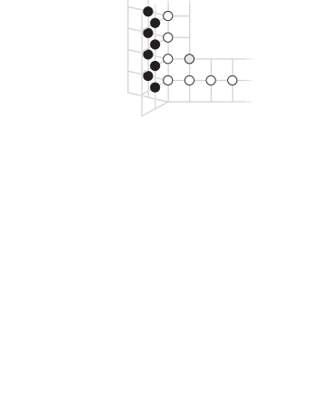
In the thermodynamic limit, solutions of the above ABA are described by complexes of Bethe roots. Among those complexes are n,n,,subscript𝑛subscript𝑛\scalebox{0.5}{\begin{picture}(7.27,0.3)\put(-1.7,2.65){$\bigcirc$}\end{picture}}_{n},\scalebox{0.6}[0.7]{\begin{picture}(7.24,0.2)\put(-1.5,0.5){$\bigtriangleup$}\end{picture}}_{n},\scalebox{0.67}{\begin{picture}(5.21,0.0)\put(-1.5,1.2){$\oplus$}\end{picture}},\scalebox{0.67}{\begin{picture}(5.21,0.0)\put(-1.5,1.2){$\otimes$}\end{picture}}, which are the same complexes as in the mirror AdS5/CFT4subscriptAdS5subscriptCFT4{\rm AdS}_{5}/{\rm CFT}_{4} (see [28]). In addition, the momentum-carrying roots u4subscript𝑢4u_{4} and u4¯subscript𝑢¯4u_{\bar{4}} form two new types of complexes, which we call Odd-Even and Even-Odd. They were recently considered in [44]. Those complexes are real-centered strings of alternating u4subscript𝑢4u_{4} and u4¯subscript𝑢¯4u_{\bar{4}} roots, adjacent roots being spaced by i𝑖i. In the Odd-Even complex, the lowest root of the string on the complex plane is u4subscript𝑢4u_{4}, while in the Even-Odd complex, the lowest root is u4¯subscript𝑢¯4u_{\bar{4}} (see Fig. 2). The list of all complexes is given in the table below.

n:string of roots:u2=u+ij,j=n22,,n22::u3=u+ij,j=n12,,n12n:pyramid:u2=u+ij,j=n22,,n22::u1=u+ij,j=n32,,n32:single fermion root:u1=u:single fermion root:u3=un:Odd-Even complex:u4=u+ijwhenθjnE=1,j=n12,,n12::u4¯=u+ijwhenθjnO=1n:Even-Odd complex:u4=u+ijwhenθjnO=1,j=n12,,n12::u4¯=u+ijwhenθjnE=1missing-subexpressionmissing-subexpressionmissing-subexpressionmissing-subexpressionmissing-subexpressionmissing-subexpression:subscript𝑛absentstring of roots:subscript𝑢2𝑢𝑖𝑗𝑗𝑛22𝑛22missing-subexpressionmissing-subexpressionmissing-subexpressionmissing-subexpressionmissing-subexpressionmissing-subexpressionmissing-subexpression:missing-subexpression:subscript𝑢3𝑢𝑖𝑗𝑗𝑛12𝑛12missing-subexpression:subscript𝑛absentpyramid:subscript𝑢2𝑢𝑖𝑗𝑗𝑛22𝑛22missing-subexpression:missing-subexpression:subscript𝑢1𝑢𝑖𝑗𝑗𝑛32𝑛32missing-subexpressionmissing-subexpressionmissing-subexpressionmissing-subexpressionmissing-subexpressionmissing-subexpressionmissing-subexpression:absentsingle fermion root:subscript𝑢1𝑢missing-subexpressionmissing-subexpressionmissing-subexpressionmissing-subexpressionmissing-subexpressionmissing-subexpressionmissing-subexpressionmissing-subexpression:absentsingle fermion root:subscript𝑢3𝑢missing-subexpressionmissing-subexpressionmissing-subexpressionmissing-subexpressionmissing-subexpressionmissing-subexpressionmissing-subexpressionmissing-subexpression:subscript𝑛absentOdd-Even complex:formulae-sequencesubscript𝑢4𝑢𝑖𝑗whensubscriptsuperscript𝜃𝐸𝑗𝑛1𝑗𝑛12𝑛12missing-subexpression:missing-subexpression:formulae-sequencesubscript𝑢¯4𝑢𝑖𝑗whensubscriptsuperscript𝜃𝑂𝑗𝑛1missing-subexpressionmissing-subexpressionmissing-subexpressionmissing-subexpressionmissing-subexpressionmissing-subexpressionmissing-subexpressionmissing-subexpression:subscript𝑛absentEven-Odd complex:formulae-sequencesubscript𝑢4𝑢𝑖𝑗whensubscriptsuperscript𝜃𝑂𝑗𝑛1𝑗𝑛12𝑛12missing-subexpression:missing-subexpression:formulae-sequencesubscript𝑢¯4𝑢𝑖𝑗whensubscriptsuperscript𝜃𝐸𝑗𝑛1missing-subexpressionmissing-subexpression\begin{array}[]{rccccc}\hline\cr\scalebox{0.5}{\begin{picture}(7.27,0.3)\put(-1.7,2.65){$\bigcirc$}\end{picture}}_{n}:&\text{string of roots}&:&u_{2}=u+ij,&j=-\frac{n-2}{2},\dots,\frac{n-2}{2}\\ \hline\cr:&&:&u_{3}=u+ij,&j=-\frac{n-1}{2},\dots,\frac{n-1}{2}\\ \scalebox{0.6}[0.7]{\begin{picture}(7.24,0.2)\put(-1.5,0.5){$\bigtriangleup$}\end{picture}}_{n}:&\text{pyramid}&:&u_{2}=u+ij,&j=-\frac{n-2}{2},\dots,\frac{n-2}{2}\\ :&&:&u_{1}=u+ij,&j=-\frac{n-3}{2},\dots,\frac{n-3}{2}\\ \hline\cr\scalebox{0.67}{\begin{picture}(5.21,0.0)\put(-1.5,1.2){$\oplus$}\end{picture}}:&\text{single fermion root}&:&u_{1}=u\\ \hline\cr\scalebox{0.67}{\begin{picture}(5.21,0.0)\put(-1.5,1.2){$\otimes$}\end{picture}}:&\text{single fermion root}&:&u_{3}=u\\ \hline\cr\scalebox{0.67}{\begin{picture}(5.21,0.0)\put(-1.5,1.2){$\blacktriangleleft$}\end{picture}}_{n}:&\text{Odd-Even complex}&:&u_{4}=u+ij\ \ \text{when}\ \ \theta^{E}_{jn}=1,&j=-\frac{n-1}{2},\dots,\frac{n-1}{2}\par\\ :&&:&u_{\bar{4}}=u+ij\ \ \text{when}\ \ \theta^{O}_{jn}=1&\\ \hline\cr\scalebox{0.67}{\begin{picture}(5.21,0.0)\put(-1.5,1.2){$\blacktriangleright$}\end{picture}}_{n}:&\text{Even-Odd complex}&:&u_{4}=u+ij\ \ \text{when}\ \ \theta^{O}_{jn}=1,&j=-\frac{n-1}{2},\dots,\frac{n-1}{2}\par\\ :&&:&u_{\bar{4}}=u+ij\ \ \text{when}\ \ \theta^{E}_{jn}=1&\\ \hline\cr\end{array}
Refer to caption Refer to caption
Odd-Even complexes 5subscript5\scalebox{0.67}{\begin{picture}(5.21,0.0)\put(-1.5,1.2){$\blacktriangleleft$}\end{picture}}_{5} and 4subscript4\scalebox{0.67}{\begin{picture}(5.21,0.0)\put(-1.5,1.2){$\blacktriangleleft$}\end{picture}}_{4} Even-Odd complexes 5subscript5\scalebox{0.67}{\begin{picture}(5.21,0.0)\put(-1.5,1.2){$\blacktriangleright$}\end{picture}}_{5} and 4subscript4\scalebox{0.67}{\begin{picture}(5.21,0.0)\put(-1.5,1.2){$\blacktriangleright$}\end{picture}}_{4}
Figure 2: Strings of alternating roots on the $\{{\rm Re}\,u,{\rm Im}\,u\}$ plane. Black circles denote $u_{4}$ roots, gray circles denote $u_{\bar{4}}$ roots. Vertical spacing between roots is $i$.

Here, $u\in\mathbb{R}$ denotes the center of a complex, notation $j=-\frac{n-1}{2},\dots,\frac{n-1}{2}$ means that $j$ takes the values $-\frac{n-1}{2},-\frac{n-3}{2},\dots,\frac{n-3}{2},\frac{n-1}{2}$, and $\theta$’s were defined in (2.16).

The energy (in our notation ipA𝑖subscriptsuperscript𝑝𝐴ip^{*}_{A}, with index A𝐴A taking the values {n,,,n,n,n}subscript𝑛subscript𝑛subscript𝑛subscript𝑛\{\scalebox{0.5}{\begin{picture}(7.27,0.3)\put(-1.7,2.65){$\bigcirc$}\end{picture}}_{n},\scalebox{0.67}{\begin{picture}(5.21,0.0)\put(-1.5,1.2){$\oplus$}\end{picture}},\scalebox{0.67}{\begin{picture}(5.21,0.0)\put(-1.5,1.2){$\otimes$}\end{picture}},\scalebox{0.6}[0.7]{\begin{picture}(7.24,0.2)\put(-1.5,0.5){$\bigtriangleup$}\end{picture}}_{n},\scalebox{0.67}{\begin{picture}(5.21,0.0)\put(-1.5,1.2){$\blacktriangleleft$}\end{picture}}_{n},\scalebox{0.67}{\begin{picture}(5.21,0.0)\put(-1.5,1.2){$\blacktriangleright$}\end{picture}}_{n}\}) which corresponds to a complex is the sum of energies of the roots in a complex, and the same is true for momentum. We have pn=pn=pnsubscriptsuperscript𝑝subscript𝑛subscriptsuperscript𝑝subscript𝑛subscriptsuperscript𝑝𝑛p^{*}_{\scalebox{0.67}{\begin{picture}(5.21,0.0)\put(-1.5,1.2){$\blacktriangleleft$}\end{picture}}_{n}}=p^{*}_{\scalebox{0.67}{\begin{picture}(5.21,0.0)\put(-1.5,1.2){$\blacktriangleright$}\end{picture}}_{n}}=p^{*}_{n}, ϵn=ϵn=ϵnsubscriptsuperscriptitalic-ϵsubscript𝑛subscriptsuperscriptitalic-ϵsubscript𝑛subscriptsuperscriptitalic-ϵ𝑛\epsilon^{*}_{\scalebox{0.67}{\begin{picture}(5.21,0.0)\put(-1.5,1.2){$\blacktriangleleft$}\end{picture}}_{n}}=\epsilon^{*}_{\scalebox{0.67}{\begin{picture}(5.21,0.0)\put(-1.5,1.2){$\blacktriangleright$}\end{picture}}_{n}}={\epsilon}^{*}_{n}, where

$$p^{*}_{n}(u)\equiv\frac{1}{i}\log\frac{x^{[+n]}}{x^{[-n]}},\ \ {\epsilon}^{*}_{n}(u)\equiv\frac{n}{2}+h(\lambda)\left(\frac{i}{x^{[+n]}}-\frac{i}{x^{[-n]}}\right),$$ (3.18)

while for other complexes, pAsubscriptsuperscript𝑝𝐴p^{*}_{A} and ϵAsubscriptsuperscriptitalic-ϵ𝐴\epsilon^{*}_{A} are zero. Note also that the only complexes with odd number of fermion roots are those denoted by ,{\scalebox{0.67}{\begin{picture}(5.21,0.0)\put(-1.5,1.2){$\oplus$}\end{picture}}},\;{\scalebox{0.67}{\begin{picture}(5.21,0.0)\put(-1.5,1.2){$\otimes$}\end{picture}}}, 2n1subscript2𝑛1{\scalebox{0.67}{\begin{picture}(5.21,0.0)\put(-1.5,1.2){$\blacktriangleleft$}\end{picture}}_{2n-1}} and 2n1subscript2𝑛1{\scalebox{0.67}{\begin{picture}(5.21,0.0)\put(-1.5,1.2){$\blacktriangleright$}\end{picture}}_{2n-1}}. Hence in our case the quantity hAsubscript𝐴h_{A} in  (3.11) has to be log(1)1\log(-1) for these complexes and log(+1)1\log(+1) otherwise.

Applying the fusion procedure to the mirror ABA equations101010an important assumption here is monotonicity, we find that in our case, kernels $K_{AB}$ entering (3.11) are given by the table below.

A\Bmmmmn+Kn1,m1Kn1+Kn1000Km100+Km11m(01)1m(01)Km100+Km11m(01)1m(01)n0Kn1+Kn1+Kn1,m1nm(01)n2,m(01)nm(01)n2,m(01)n0n1(10)n1(10)nm(10)n,m2(10)𝒯nm𝒯nmn0n1(10)n1(10)nm(10)n,m2(10)𝒯nm𝒯nmmissing-subexpressionmissing-subexpressionmissing-subexpressionmissing-subexpressionmissing-subexpressionmissing-subexpressionmissing-subexpression\𝐴𝐵subscript𝑚subscript𝑚subscript𝑚subscript𝑚missing-subexpressionmissing-subexpressionmissing-subexpressionmissing-subexpressionmissing-subexpressionmissing-subexpressionmissing-subexpressionmissing-subexpressionmissing-subexpressionmissing-subexpressionmissing-subexpressionmissing-subexpressionmissing-subexpressionmissing-subexpressionsubscript𝑛subscript𝐾𝑛1𝑚1subscript𝐾𝑛1subscript𝐾𝑛1000missing-subexpressionmissing-subexpressionmissing-subexpressionmissing-subexpressionmissing-subexpressionmissing-subexpressionmissing-subexpressionsubscript𝐾𝑚100subscript𝐾𝑚1subscriptsuperscript011𝑚subscriptsuperscript011𝑚missing-subexpressionmissing-subexpressionmissing-subexpressionmissing-subexpressionmissing-subexpressionmissing-subexpressionmissing-subexpressionsubscript𝐾𝑚100subscript𝐾𝑚1subscriptsuperscript011𝑚subscriptsuperscript011𝑚missing-subexpressionmissing-subexpressionmissing-subexpressionmissing-subexpressionmissing-subexpressionmissing-subexpressionmissing-subexpressionsubscript𝑛0subscript𝐾𝑛1subscript𝐾𝑛1subscript𝐾𝑛1𝑚1subscriptsuperscript01𝑛𝑚subscriptsuperscript01𝑛2𝑚subscriptsuperscript01𝑛𝑚subscriptsuperscript01𝑛2𝑚missing-subexpressionmissing-subexpressionmissing-subexpressionmissing-subexpressionmissing-subexpressionmissing-subexpressionmissing-subexpressionsubscript𝑛0subscriptsuperscript10𝑛1subscriptsuperscript10𝑛1subscriptsuperscript10𝑛𝑚subscriptsuperscript10𝑛𝑚2subscriptsuperscript𝒯𝑛𝑚superscriptsubscript𝒯𝑛𝑚bottommissing-subexpressionmissing-subexpressionmissing-subexpressionmissing-subexpressionmissing-subexpressionmissing-subexpressionmissing-subexpressionsubscript𝑛0subscriptsuperscript10𝑛1subscriptsuperscript10𝑛1subscriptsuperscript10𝑛𝑚subscriptsuperscript10𝑛𝑚2superscriptsubscript𝒯𝑛𝑚bottomsuperscriptsubscript𝒯𝑛𝑚\displaystyle{\footnotesize\begin{array}[]{|l@{}||l@{}|l|l|l|l|l|}\hline\cr A\backslash B&\scalebox{0.5}{\begin{picture}(7.27,0.3)\put(-1.7,2.65){$\bigcirc$}\end{picture}}_{m}&\scalebox{0.67}{\begin{picture}(5.21,0.0)\put(-1.5,1.2){$\oplus$}\end{picture}}&\scalebox{0.67}{\begin{picture}(5.21,0.0)\put(-1.5,1.2){$\otimes$}\end{picture}}&\scalebox{0.6}[0.7]{\begin{picture}(7.24,0.2)\put(-1.5,0.5){$\bigtriangleup$}\end{picture}}_{m}&\scalebox{0.67}{\begin{picture}(5.21,0.0)\put(-1.5,1.2){$\blacktriangleleft$}\end{picture}}_{m}&\scalebox{0.67}{\begin{picture}(5.21,0.0)\put(-1.5,1.2){$\blacktriangleright$}\end{picture}}_{m}\\ \hline\cr\hline\cr\scalebox{0.5}{\begin{picture}(7.27,0.3)\put(-1.7,2.65){$\bigcirc$}\end{picture}}_{n}&+K_{n-1,m-1}&-K_{n-1}&+K_{n-1}&0&0&0\\ \hline\cr\scalebox{0.67}{\begin{picture}(5.21,0.0)\put(-1.5,1.2){$\oplus$}\end{picture}}&-K_{m-1}&0&0&+K_{m-1}&-\mathcal{B}^{(01)}_{1m}&-\mathcal{B}^{(01)}_{1m}\\ \hline\cr\scalebox{0.67}{\begin{picture}(5.21,0.0)\put(-1.5,1.2){$\otimes$}\end{picture}}&-K_{m-1}&0&0&+K_{m-1}&-\mathcal{R}^{(01)}_{1m}&-\mathcal{R}^{(01)}_{1m}\\ \hline\cr\scalebox{0.6}[0.7]{\begin{picture}(7.24,0.2)\put(-1.5,0.5){$\bigtriangleup$}\end{picture}}_{n}&0&-K_{n-1}&+K_{n-1}&+K_{n-1,m-1}&-\mathcal{R}^{(01)}_{nm}-\mathcal{B}^{(01)}_{n-2,m}&-\mathcal{R}^{(01)}_{nm}-\mathcal{B}^{(01)}_{n-2,m}\\ \hline\cr\scalebox{0.67}{\begin{picture}(5.21,0.0)\put(-1.5,1.2){$\blacktriangleleft$}\end{picture}}_{n}&0&\mathcal{B}^{(10)}_{n1}&-\mathcal{R}^{(10)}_{n1}&-\mathcal{R}^{(10)}_{nm}-\mathcal{B}^{(10)}_{n,m-2}&\begin{array}[]{l}-{\cal T}^{\|}_{nm}\end{array}&\begin{array}[]{l}-{\cal T}_{nm}^{\bot}\end{array}\\ \hline\cr\scalebox{0.67}{\begin{picture}(5.21,0.0)\put(-1.5,1.2){$\blacktriangleright$}\end{picture}}_{n}&0&\mathcal{B}^{(10)}_{n1}&-\mathcal{R}^{(10)}_{n1}&-\mathcal{R}^{(10)}_{nm}-\mathcal{B}^{(10)}_{n,m-2}&\begin{array}[]{l}-{\cal T}_{nm}^{\bot}\end{array}&\begin{array}[]{l}-{\cal T}_{nm}^{\|}\end{array}\\ \hline\cr\end{array}} (3.30)

Some of those kernels are the same as in the ${\rm AdS}_{5}/{\rm CFT}_{4}$ case [24], and we list them in Appendix A. The new kernels are

$\displaystyle{\cal T}_{nm}^{\|}$ $\displaystyle\equiv$ $\displaystyle\mathcal{B}^{(11)}_{nm}+\tilde{\cal S}_{nm}-K_{nm}^{\|},$ (3.31)
$\displaystyle{\cal T}_{nm}^{\bot}$ $\displaystyle\equiv$ $\displaystyle\mathcal{B}^{(11)}_{nm}+\tilde{\cal S}_{nm}-K_{nm}^{\bot},$ (3.32)

where

$\displaystyle K^{\|}_{nm}(u,v)$ $\displaystyle\equiv$ $\displaystyle\sum_{l=-\frac{n-1}{2}}^{\frac{n-1}{2}}\sum_{k=-\frac{m-1}{2}}^{\frac{m-1}{2}}K_{2}(u-v+i(l-k))\left(\theta^{\rm E}_{ln}\theta^{\rm O}_{km}+\theta^{\rm O}_{ln}\theta^{\rm E}_{km}\right),$ (3.33)
$\displaystyle K^{\bot}_{nm}(u,v)$ $\displaystyle\equiv$ $\displaystyle\sum_{l=-\frac{n-1}{2}}^{\frac{n-1}{2}}\sum_{k=-\frac{m-1}{2}}^{\frac{m-1}{2}}K_{2}(u-v+i(l-k))\left(\theta^{\rm E}_{ln}\theta^{\rm E}_{km}+\theta^{\rm O}_{ln}\theta^{\rm O}_{km}\right).$ (3.34)

Let us also introduce the functions $Y_{A}$, which will turn out to be the functions which enter the Y-system:

{Yn,Y,1Y,1Yn,1Yn,1Yn}subscript𝑌subscript𝑛subscript𝑌1subscript𝑌1subscript𝑌subscript𝑛1subscript𝑌subscript𝑛1subscript𝑌subscript𝑛\displaystyle\left\{{Y}_{\scalebox{0.5}{\begin{picture}(7.27,0.3)\put(-1.7,2.65){$\bigcirc$}\end{picture}}_{n}},Y_{\scalebox{0.67}{\begin{picture}(5.21,0.0)\put(-1.5,1.2){$\oplus$}\end{picture}}},\frac{1}{Y_{\scalebox{0.67}{\begin{picture}(5.21,0.0)\put(-1.5,1.2){$\otimes$}\end{picture}}}},\frac{1}{Y_{\scalebox{0.6}[0.7]{\begin{picture}(7.24,0.2)\put(-1.5,0.5){$\bigtriangleup$}\end{picture}}_{n}}},\frac{1}{Y_{\scalebox{0.67}{\begin{picture}(5.21,0.0)\put(-1.5,1.2){$\blacktriangleleft$}\end{picture}}_{n}}},\frac{1}{Y_{\scalebox{0.67}{\begin{picture}(5.21,0.0)\put(-1.5,1.2){$\blacktriangleright$}\end{picture}}_{n}}}\right\} \displaystyle\equiv {𝒴n,𝒴,𝒴,𝒴n,𝒴n,𝒴n}subscript𝒴subscript𝑛subscript𝒴subscript𝒴subscript𝒴subscript𝑛subscript𝒴subscript𝑛subscript𝒴subscript𝑛\displaystyle\left\{\mathcal{Y}_{\scalebox{0.5}{\begin{picture}(7.27,0.3)\put(-1.7,2.65){$\bigcirc$}\end{picture}}_{n}},\mathcal{Y}_{\scalebox{0.67}{\begin{picture}(5.21,0.0)\put(-1.5,1.2){$\oplus$}\end{picture}}},\mathcal{Y}_{\scalebox{0.67}{\begin{picture}(5.21,0.0)\put(-1.5,1.2){$\otimes$}\end{picture}}},\mathcal{Y}_{\scalebox{0.6}[0.7]{\begin{picture}(7.24,0.2)\put(-1.5,0.5){$\bigtriangleup$}\end{picture}}_{n}},\mathcal{Y}_{\scalebox{0.67}{\begin{picture}(5.21,0.0)\put(-1.5,1.2){$\blacktriangleleft$}\end{picture}}_{n}},\mathcal{Y}_{\scalebox{0.67}{\begin{picture}(5.21,0.0)\put(-1.5,1.2){$\blacktriangleright$}\end{picture}}_{n}}\right\} (3.35)

(We recall that $\mathcal{Y}_{A}\equiv\frac{\bar{\rho}_{A}}{\rho_{A}}$.)


We can write the TBA equations for the ground state in the following way:

logYsubscript𝑌\displaystyle\log Y_{\scalebox{0.67}{\begin{picture}(5.21,0.0)\put(-1.5,1.2){$\otimes$}\end{picture}}} =\displaystyle= +Km1log1+1/Ym1+Ym+1m(01)log(1+Ym)(1+Ym)+iπsubscript𝐾𝑚111subscript𝑌subscript𝑚1subscript𝑌subscript𝑚superscriptsubscript1𝑚011subscript𝑌subscript𝑚1subscript𝑌subscript𝑚𝑖𝜋\displaystyle+K_{m-1}*\log\frac{1+1/Y_{\scalebox{0.5}{\begin{picture}(7.27,0.3)\put(-1.7,2.65){$\bigcirc$}\end{picture}}_{m}}}{1+Y_{\scalebox{0.6}[0.7]{\begin{picture}(7.24,0.2)\put(-1.5,0.5){$\bigtriangleup$}\end{picture}}_{m}}}+\mathcal{{R}}_{1m}^{(01)}*\log(1+Y_{\scalebox{0.67}{\begin{picture}(5.21,0.0)\put(-1.5,1.2){$\blacktriangleleft$}\end{picture}}_{m}})(1+Y_{\scalebox{0.67}{\begin{picture}(5.21,0.0)\put(-1.5,1.2){$\blacktriangleright$}\end{picture}}_{m}})+i\pi (3.36)
logYsubscript𝑌\displaystyle\log Y_{\scalebox{0.67}{\begin{picture}(5.21,0.0)\put(-1.5,1.2){$\oplus$}\end{picture}}} =\displaystyle= Km1log1+1/Ym1+Ym1m(01)log(1+Ym)(1+Ym)iπsubscript𝐾𝑚111subscript𝑌subscript𝑚1subscript𝑌subscript𝑚superscriptsubscript1𝑚011subscript𝑌subscript𝑚1subscript𝑌subscript𝑚𝑖𝜋\displaystyle-K_{m-1}*\log\frac{1+1/Y_{\scalebox{0.5}{\begin{picture}(7.27,0.3)\put(-1.7,2.65){$\bigcirc$}\end{picture}}_{m}}}{1+Y_{\scalebox{0.6}[0.7]{\begin{picture}(7.24,0.2)\put(-1.5,0.5){$\bigtriangleup$}\end{picture}}_{m}}}-\mathcal{{B}}_{1m}^{(01)}*\log(1+Y_{\scalebox{0.67}{\begin{picture}(5.21,0.0)\put(-1.5,1.2){$\blacktriangleleft$}\end{picture}}_{m}})(1+Y_{\scalebox{0.67}{\begin{picture}(5.21,0.0)\put(-1.5,1.2){$\blacktriangleright$}\end{picture}}_{m}})-i\pi (3.37)
logYnsubscript𝑌subscript𝑛\displaystyle\log Y_{{\scalebox{0.6}[0.7]{\begin{picture}(7.24,0.2)\put(-1.5,0.5){$\bigtriangleup$}\end{picture}}}_{n}} =\displaystyle= Kn1,m1log(1+Ym)Kn1log(1+Y)\displaystyle-K_{n-1,m-1}*\log(1+Y_{{\scalebox{0.6}[0.7]{\begin{picture}(7.24,0.2)\put(-1.5,0.5){$\bigtriangleup$}\end{picture}}}_{m}})-K_{n-1}{\circlearrowright*\hskip 0.56905pt}\log({1+Y_{\scalebox{0.67}{\begin{picture}(5.21,0.0)\put(-1.5,1.2){$\otimes$}\end{picture}}}})
+\displaystyle+ (nm(01)+n2,m(01))log(1+Ym)(1+Ym)subscriptsuperscript01𝑛𝑚subscriptsuperscript01𝑛2𝑚1subscript𝑌subscript𝑚1subscript𝑌subscript𝑚\displaystyle\left({\cal{R}}^{(01)}_{nm}+{\cal{B}}^{(01)}_{n-2,m}\right)*\log(1+Y_{\scalebox{0.67}{\begin{picture}(5.21,0.0)\put(-1.5,1.2){$\blacktriangleleft$}\end{picture}}_{m}})(1+Y_{\scalebox{0.67}{\begin{picture}(5.21,0.0)\put(-1.5,1.2){$\blacktriangleright$}\end{picture}}_{m}})
logYnsubscript𝑌subscript𝑛\displaystyle\log Y_{{\scalebox{0.5}{\begin{picture}(7.27,0.3)\put(-1.7,2.65){$\bigcirc$}\end{picture}}}_{n}} =\displaystyle= Kn1,m1log(1+1/Ym)+Kn1log(1+Y)\displaystyle K_{n-1,m-1}*\log(1+1/Y_{{\scalebox{0.5}{\begin{picture}(7.27,0.3)\put(-1.7,2.65){$\bigcirc$}\end{picture}}}_{m}})+K_{n-1}{\circlearrowright*\hskip 0.56905pt}\log({1+Y_{\scalebox{0.67}{\begin{picture}(5.21,0.0)\put(-1.5,1.2){$\otimes$}\end{picture}}}}) (3.39)
logYnsubscript𝑌subscript𝑛\displaystyle\log Y_{{\scalebox{0.67}{\begin{picture}(5.21,0.0)\put(-1.5,1.2){$\blacktriangleleft$}\end{picture}}}_{n}} =\displaystyle= iLpn+𝒯nmlog(1+Ym)+𝒯nmlog(1+Ym)+iπn𝑖𝐿subscriptsuperscript𝑝𝑛superscriptsubscript𝒯𝑛𝑚1subscript𝑌subscript𝑚superscriptsubscript𝒯𝑛𝑚bottom1subscript𝑌subscript𝑚𝑖𝜋𝑛\displaystyle-iLp^{*}_{n}+{\cal T}_{nm}^{\|}*\log(1+Y_{\scalebox{0.67}{\begin{picture}(5.21,0.0)\put(-1.5,1.2){$\blacktriangleleft$}\end{picture}}_{m}})+{\cal T}_{nm}^{\bot}*\log(1+Y_{\scalebox{0.67}{\begin{picture}(5.21,0.0)\put(-1.5,1.2){$\blacktriangleright$}\end{picture}}_{m}})+i\pi n
+\displaystyle+ n1(10)log(1+Y)+(nm(10)+n,m2(10))log(1+Ym)\displaystyle{\cal{R}}_{n1}^{(10)}{\circlearrowright*\hskip 0.56905pt}\log(1+Y_{\scalebox{0.67}{\begin{picture}(5.21,0.0)\put(-1.5,1.2){$\otimes$}\end{picture}}})+\left({\cal{R}}_{nm}^{(10)}+{\cal{B}}_{n,m-2}^{(10)}\right)*\log(1+Y_{\scalebox{0.6}[0.7]{\begin{picture}(7.24,0.2)\put(-1.5,0.5){$\bigtriangleup$}\end{picture}}_{m}})
logYnsubscript𝑌subscript𝑛\displaystyle\log Y_{{\scalebox{0.67}{\begin{picture}(5.21,0.0)\put(-1.5,1.2){$\blacktriangleright$}\end{picture}}}_{n}} =\displaystyle= iLpn+𝒯nmlog(1+Ym)+𝒯nmlog(1+Ym)+iπn𝑖𝐿subscriptsuperscript𝑝𝑛superscriptsubscript𝒯𝑛𝑚1subscript𝑌subscript𝑚superscriptsubscript𝒯𝑛𝑚bottom1subscript𝑌subscript𝑚𝑖𝜋𝑛\displaystyle-iLp^{*}_{n}+{\cal T}_{nm}^{\|}*\log(1+Y_{\scalebox{0.67}{\begin{picture}(5.21,0.0)\put(-1.5,1.2){$\blacktriangleright$}\end{picture}}_{m}})+{\cal T}_{nm}^{\bot}*\log(1+Y_{\scalebox{0.67}{\begin{picture}(5.21,0.0)\put(-1.5,1.2){$\blacktriangleleft$}\end{picture}}_{m}})+i\pi n
+\displaystyle+ n1(10)log(1+Y)+(nm(10)+n,m2(10))log(1+Ym)\displaystyle{\cal{R}}_{n1}^{(10)}{\circlearrowright*\hskip 0.56905pt}\log(1+Y_{\scalebox{0.67}{\begin{picture}(5.21,0.0)\put(-1.5,1.2){$\otimes$}\end{picture}}})+\left({\cal{R}}_{nm}^{(10)}+{\cal{B}}_{n,m-2}^{(10)}\right)*\log(1+Y_{\scalebox{0.6}[0.7]{\begin{picture}(7.24,0.2)\put(-1.5,0.5){$\bigtriangleup$}\end{picture}}_{m}})

where * denotes integration over the second variable, as in (3.11). Summation over the repeated index m𝑚m is assumed with m2𝑚2m\geq 2 for msubscript𝑚\scalebox{0.6}[0.7]{\begin{picture}(7.24,0.2)\put(-1.5,0.5){$\bigtriangleup$}\end{picture}}_{m} and msubscript𝑚\scalebox{0.5}{\begin{picture}(7.27,0.3)\put(-1.7,2.65){$\bigcirc$}\end{picture}}_{m}, and m1𝑚1m\geq 1 for m,msubscript𝑚subscript𝑚\scalebox{0.67}{\begin{picture}(5.21,0.0)\put(-1.5,1.2){$\blacktriangleleft$}\end{picture}}_{m},\scalebox{0.67}{\begin{picture}(5.21,0.0)\put(-1.5,1.2){$\blacktriangleright$}\end{picture}}_{m}.

Range of integration for fermions is limited to 2h<u<2h2𝑢2-2h<u<2h. Notice that from (3.36) and (3.37) we can see that 1Y1subscript𝑌\frac{1}{Y_{\scalebox{0.67}{\begin{picture}(5.21,0.0)\put(-1.5,1.2){$\oplus$}\end{picture}}}} is the analytical continuation of Ysubscript𝑌Y_{\scalebox{0.67}{\begin{picture}(5.21,0.0)\put(-1.5,1.2){$\otimes$}\end{picture}}} across the cut u(,2h)(2h,+)𝑢22u\in(-\infty,-2h)\cup(2h,+\infty). For the convolutions with fermions we introduce the convolutions absent{\circlearrowright*\hskip 0.56905pt} which should be understood in the sense of a B-cycle (see [24]), e.g.

Kn1log(1+Y)2h2hdvKn1log1+Y1+1/Y,\displaystyle K_{n-1}{\circlearrowright*\hskip 0.56905pt}\log({1+Y_{\scalebox{0.67}{\begin{picture}(5.21,0.0)\put(-1.5,1.2){$\otimes$}\end{picture}}}})\equiv\int_{-2h}^{2h}dvK_{n-1}\log\frac{1+Y_{\scalebox{0.67}{\begin{picture}(5.21,0.0)\put(-1.5,1.2){$\otimes$}\end{picture}}}}{1+1/Y_{\scalebox{0.67}{\begin{picture}(5.21,0.0)\put(-1.5,1.2){$\oplus$}\end{picture}}}}\;, (3.42)
(n0)log(1+Y)2h2hdv[(n0)log(1+Y)(n0)log(1+1/Y)].\displaystyle{\cal R}^{(n0)}{\circlearrowright*\hskip 0.56905pt}\log(1+Y_{\scalebox{0.67}{\begin{picture}(5.21,0.0)\put(-1.5,1.2){$\otimes$}\end{picture}}})\equiv\int_{-2h}^{2h}dv\left[{\cal R}^{(n0)}\log(1+Y_{\scalebox{0.67}{\begin{picture}(5.21,0.0)\put(-1.5,1.2){$\otimes$}\end{picture}}})-{\cal B}^{(n0)}\log(1+1/Y_{\scalebox{0.67}{\begin{picture}(5.21,0.0)\put(-1.5,1.2){$\oplus$}\end{picture}}})\right]\;.

Remarkably, the combination $\mathcal{B}^{(11)}_{nm}+\tilde{\cal S}_{nm}$, which is part of the kernels ${\cal T}_{nm}^{\bot}$ and ${\cal T}_{nm}^{\|}$, has only two branch cuts for each of the variables $u$ and $v$. This follows from the integral representation

$\displaystyle{\cal\tilde{S}}_{nm}(u,v)+{\cal B}_{nm}^{(11)}(u,v)=$ (3.43)
$\displaystyle-\sum_{a=1}^{\infty}\int\left[{\cal B}^{(10)}_{n1}\left(u,w+ia/2\right){\cal B}_{1m}^{(01)}\left(w-ia/2,v\right)+{\cal B}^{(10)}_{n1}\left(u,w-ia/2\right){\cal B}_{1m}^{(01)}\left(w+ia/2,v\right)\right]dw,$

which can be derived using the results obtained in [24, 25] (see Appendix A). As a consequence, the functions Yn(u)subscript𝑌subscript𝑛𝑢Y_{\scalebox{0.67}{\begin{picture}(5.21,0.0)\put(-1.5,1.2){$\blacktriangleleft$}\end{picture}}_{n}}(u) and Yn(u)subscript𝑌subscript𝑛𝑢Y_{\scalebox{0.67}{\begin{picture}(5.21,0.0)\put(-1.5,1.2){$\blacktriangleright$}\end{picture}}_{n}}(u) (see (3.1), (3.1)) should not have branch cuts for in/2<Imu<in/2𝑖𝑛2Im𝑢𝑖𝑛2-in/2<{\rm Im}\,u<in/2.

In the next section we will establish a relation between the above equations and the ${\rm AdS}_{4}/{\rm CFT}_{3}$ Y-system.

3.2 Y-system from TBA equations

In this section we show that solutions of ground state TBA equations satisfy the ${\rm AdS}_{4}/{\rm CFT}_{3}$ Y-system (1.2)–(1.4) described in the introduction. This derivation of the Y-system is similar to the ${\rm AdS}_{5}/{\rm CFT}_{4}$ case [24]. First, we identify the $Y_{A}$ functions in TBA equations with the Y-system functions $Y_{a,s}$. We set

{Yn,Y,Y,Yn}={Y1,n,Y2,2,Y1,1,Yn,1}.subscript𝑌subscript𝑛subscript𝑌subscript𝑌subscript𝑌subscript𝑛subscript𝑌1𝑛subscript𝑌22subscript𝑌11subscript𝑌𝑛1\left\{Y_{\scalebox{0.5}{\begin{picture}(7.27,0.3)\put(-1.7,2.65){$\bigcirc$}\end{picture}}_{n}},Y_{\scalebox{0.67}{\begin{picture}(5.21,0.0)\put(-1.5,1.2){$\oplus$}\end{picture}}},Y_{\scalebox{0.67}{\begin{picture}(5.21,0.0)\put(-1.5,1.2){$\otimes$}\end{picture}}},Y_{\scalebox{0.6}[0.7]{\begin{picture}(7.24,0.2)\put(-1.5,0.5){$\bigtriangleup$}\end{picture}}_{n}}\right\}=\left\{Y_{1,n},Y_{2,2},Y_{1,1},Y_{n,1}\right\}. (3.44)

Let us introduce the discrete Laplacian operator

$$\Delta K_{n}(u)\equiv K_{n}(u+i/2-i0)+K_{n}(u-i/2+i0)-K_{n+1}(u)-K_{n-1}(u).$$

Following [24], we apply this operator to the l.h.s. of the TBA equations, acting on the free index $n$ and the free variable $u$. The action of this Laplacian on some of our kernels has been computed in [24]:

$\displaystyle\Delta K_{n}(u)$ $\displaystyle=$ $\displaystyle\delta_{n,1}\delta(u)$ (3.45)
$\displaystyle\Delta K_{nm}(v-u)$ $\displaystyle=$ $\displaystyle\Delta{\cal R}^{(11)}_{nm}(v,u)=\delta_{n,m+1}\delta(v-u)+\delta_{n,m-1}\delta(v-u)$ (3.46)
$\displaystyle\Delta{\cal R}^{(01)}_{nm}(v,u)$ $\displaystyle=$ $\displaystyle\Delta{\cal R}^{(10)}_{nm}(v,u)=\delta_{n,m}\delta(v-u)$ (3.47)
$\displaystyle\Delta{\cal B}_{nm}$ $\displaystyle=$ $\displaystyle 0,\ \ \ \Delta\tilde{\cal S}_{nm}=0\;.$ (3.48)

The new kernels ${\cal T}_{nm}^{\|}$ and ${\cal T}_{nm}^{\bot}$ satisfy relations of a new type, which are not written in terms of the Laplacian:

$\displaystyle{\cal T}_{nm}^{\bot}(u\!+\!\tfrac{i-i0}{2},v)\!+\!{\cal T}_{nm}^{\|}(u\!-\!\tfrac{i-i0}{2},v)\!-\!{\cal T}_{n+1,m}^{\|}(u,v)\!-\!{\cal T}_{n-1,m}^{\bot}(u,v)\!=\!-\delta_{n,m-1}\delta(u\!-\!v)$ (3.49)
$\displaystyle{\cal T}_{nm}^{\|}(u\!+\!\tfrac{i-i0}{2},v)\!+\!{\cal T}_{nm}^{\bot}(u\!-\!\tfrac{i-i0}{2},v)\!-\!{\cal T}_{n+1,m}^{\bot}(u,v)\!-\!{\cal T}_{n-1,m}^{\|}(u,v)\!=\!-\delta_{n-1,m}\delta(u\!-\!v)\;.$

Using those identities, we obtain from the TBA equations a set of simpler equations for the functions $Y_{A}$. This closely follows [24]. For example, applying the Laplacian to the l.h.s of (3.39), we get

logYn+YnYn+1Yn1=log(1+1/Yn+1)(1+1/Yn1),n>2formulae-sequencesuperscriptsubscript𝑌subscript𝑛superscriptsubscript𝑌subscript𝑛subscript𝑌subscript𝑛1subscript𝑌subscript𝑛111subscript𝑌subscript𝑛111subscript𝑌subscript𝑛1𝑛2\log\frac{Y_{{\scalebox{0.5}{\begin{picture}(7.27,0.3)\put(-1.7,2.65){$\bigcirc$}\end{picture}}}_{n}}^{+}Y_{{\scalebox{0.5}{\begin{picture}(7.27,0.3)\put(-1.7,2.65){$\bigcirc$}\end{picture}}}_{n}}^{-}}{Y_{\scalebox{0.5}{\begin{picture}(7.27,0.3)\put(-1.7,2.65){$\bigcirc$}\end{picture}}_{n}+1}Y_{\scalebox{0.5}{\begin{picture}(7.27,0.3)\put(-1.7,2.65){$\bigcirc$}\end{picture}}_{n}-1}}=\log(1+1/Y_{{\scalebox{0.5}{\begin{picture}(7.27,0.3)\put(-1.7,2.65){$\bigcirc$}\end{picture}}}_{n+1}})(1+1/Y_{{\scalebox{0.5}{\begin{picture}(7.27,0.3)\put(-1.7,2.65){$\bigcirc$}\end{picture}}}_{n-1}})\,\,,\,\,n>2 (3.50)

or, equivalently,

logYn+Yn=log(1+Yn+1)(1+Yn1),n>2.formulae-sequencesuperscriptsubscript𝑌subscript𝑛superscriptsubscript𝑌subscript𝑛1subscript𝑌subscript𝑛11subscript𝑌subscript𝑛1𝑛2\log{Y_{{\scalebox{0.5}{\begin{picture}(7.27,0.3)\put(-1.7,2.65){$\bigcirc$}\end{picture}}}_{n}}^{+}Y_{{\scalebox{0.5}{\begin{picture}(7.27,0.3)\put(-1.7,2.65){$\bigcirc$}\end{picture}}}_{n}}^{-}}=\log(1+Y_{{\scalebox{0.5}{\begin{picture}(7.27,0.3)\put(-1.7,2.65){$\bigcirc$}\end{picture}}}_{n+1}})(1+Y_{{\scalebox{0.5}{\begin{picture}(7.27,0.3)\put(-1.7,2.65){$\bigcirc$}\end{picture}}}_{n-1}})\,\,,\,\,n>2. (3.51)

For $n=2$ we obtain

logY2+Y2=log(1+Y)(1+Y3)1+1/Y.superscriptsubscript𝑌subscript2superscriptsubscript𝑌subscript21subscript𝑌1subscript𝑌subscript311subscript𝑌\log{Y_{{\scalebox{0.5}{\begin{picture}(7.27,0.3)\put(-1.7,2.65){$\bigcirc$}\end{picture}}}_{2}}^{+}Y_{{\scalebox{0.5}{\begin{picture}(7.27,0.3)\put(-1.7,2.65){$\bigcirc$}\end{picture}}}_{2}}^{-}}=\log\frac{(1+Y_{\scalebox{0.67}{\begin{picture}(5.21,0.0)\put(-1.5,1.2){$\otimes$}\end{picture}}})(1+Y_{{\scalebox{0.5}{\begin{picture}(7.27,0.3)\put(-1.7,2.65){$\bigcirc$}\end{picture}}}_{3}})}{1+1/Y_{\scalebox{0.67}{\begin{picture}(5.21,0.0)\put(-1.5,1.2){$\oplus$}\end{picture}}}}. (3.52)

Equations (3.36) and (3.1) can be treated in a similar way. We get an equation for Ysubscript𝑌Y_{\scalebox{0.67}{\begin{picture}(5.21,0.0)\put(-1.5,1.2){$\otimes$}\end{picture}}}

logY+Y=log(1+Y2)(1+Y1)(1+Y1)1+1/Y2,superscriptsubscript𝑌superscriptsubscript𝑌1subscript𝑌subscript21subscript𝑌subscript11subscript𝑌subscript111subscript𝑌subscript2\log{Y_{\scalebox{0.67}{\begin{picture}(5.21,0.0)\put(-1.5,1.2){$\otimes$}\end{picture}}}^{+}Y_{\scalebox{0.67}{\begin{picture}(5.21,0.0)\put(-1.5,1.2){$\otimes$}\end{picture}}}^{-}}=\log\frac{(1+Y_{\scalebox{0.5}{\begin{picture}(7.27,0.3)\put(-1.7,2.65){$\bigcirc$}\end{picture}}_{2}})(1+Y_{\scalebox{0.67}{\begin{picture}(5.21,0.0)\put(-1.5,1.2){$\blacktriangleleft$}\end{picture}}_{1}})(1+Y_{\scalebox{0.67}{\begin{picture}(5.21,0.0)\put(-1.5,1.2){$\blacktriangleright$}\end{picture}}_{1}})}{1+1/Y_{\scalebox{0.6}[0.7]{\begin{picture}(7.24,0.2)\put(-1.5,0.5){$\bigtriangleup$}\end{picture}}_{2}}}, (3.53)

and also equations for Ynsubscript𝑌subscript𝑛Y_{{\scalebox{0.6}[0.7]{\begin{picture}(7.24,0.2)\put(-1.5,0.5){$\bigtriangleup$}\end{picture}}}_{n}}:

logYn+YnYn+1Yn1=log(1+Yn)(1+Yn)(1+Yn+1)(1+Yn1),n>2formulae-sequencesuperscriptsubscript𝑌subscript𝑛superscriptsubscript𝑌subscript𝑛subscript𝑌subscript𝑛1subscript𝑌subscript𝑛11subscript𝑌subscript𝑛1subscript𝑌subscript𝑛1subscript𝑌subscript𝑛11subscript𝑌subscript𝑛1𝑛2\log\frac{Y_{{\scalebox{0.6}[0.7]{\begin{picture}(7.24,0.2)\put(-1.5,0.5){$\bigtriangleup$}\end{picture}}}_{n}}^{+}Y_{{\scalebox{0.6}[0.7]{\begin{picture}(7.24,0.2)\put(-1.5,0.5){$\bigtriangleup$}\end{picture}}}_{n}}^{-}}{Y_{{\scalebox{0.6}[0.7]{\begin{picture}(7.24,0.2)\put(-1.5,0.5){$\bigtriangleup$}\end{picture}}}_{n+1}}Y_{{\scalebox{0.6}[0.7]{\begin{picture}(7.24,0.2)\put(-1.5,0.5){$\bigtriangleup$}\end{picture}}}_{n-1}}}=\log\frac{(1+Y_{\scalebox{0.67}{\begin{picture}(5.21,0.0)\put(-1.5,1.2){$\blacktriangleleft$}\end{picture}}_{n}})(1+Y_{\scalebox{0.67}{\begin{picture}(5.21,0.0)\put(-1.5,1.2){$\blacktriangleright$}\end{picture}}_{n}})}{(1+Y_{{\scalebox{0.6}[0.7]{\begin{picture}(7.24,0.2)\put(-1.5,0.5){$\bigtriangleup$}\end{picture}}}_{n+1}})(1+Y_{{\scalebox{0.6}[0.7]{\begin{picture}(7.24,0.2)\put(-1.5,0.5){$\bigtriangleup$}\end{picture}}}_{n-1}})}\,\,,\,\,n>2 (3.54)
logY2+Y2Y3superscriptsubscript𝑌subscript2superscriptsubscript𝑌subscript2subscript𝑌subscript3\displaystyle\log\frac{Y_{\scalebox{0.6}[0.7]{\begin{picture}(7.24,0.2)\put(-1.5,0.5){$\bigtriangleup$}\end{picture}}_{2}}^{+}Y_{\scalebox{0.6}[0.7]{\begin{picture}(7.24,0.2)\put(-1.5,0.5){$\bigtriangleup$}\end{picture}}_{2}}^{-}}{Y_{\scalebox{0.6}[0.7]{\begin{picture}(7.24,0.2)\put(-1.5,0.5){$\bigtriangleup$}\end{picture}}_{3}}} =\displaystyle= log(1+Y)(1+Y2)(1+Y2)Y(1+Y3)(1+Y)1subscript𝑌1subscript𝑌subscript21subscript𝑌subscript2subscript𝑌1subscript𝑌subscript31subscript𝑌\displaystyle\log\frac{(1+Y_{\scalebox{0.67}{\begin{picture}(5.21,0.0)\put(-1.5,1.2){$\oplus$}\end{picture}}})(1+Y_{\scalebox{0.67}{\begin{picture}(5.21,0.0)\put(-1.5,1.2){$\blacktriangleleft$}\end{picture}}_{2}})(1+Y_{\scalebox{0.67}{\begin{picture}(5.21,0.0)\put(-1.5,1.2){$\blacktriangleright$}\end{picture}}_{2}})Y_{\scalebox{0.67}{\begin{picture}(5.21,0.0)\put(-1.5,1.2){$\otimes$}\end{picture}}}}{(1+Y_{\scalebox{0.6}[0.7]{\begin{picture}(7.24,0.2)\put(-1.5,0.5){$\bigtriangleup$}\end{picture}}_{3}})(1+Y_{\scalebox{0.67}{\begin{picture}(5.21,0.0)\put(-1.5,1.2){$\otimes$}\end{picture}}})}
\displaystyle- logYY+m(1m(01)1m(01))log(1+Ym)(1+Ym)subscript𝑌subscript𝑌subscript𝑚subscriptsuperscript011𝑚subscriptsuperscript011𝑚1subscript𝑌subscript𝑚1subscript𝑌subscript𝑚\displaystyle\log Y_{\scalebox{0.67}{\begin{picture}(5.21,0.0)\put(-1.5,1.2){$\otimes$}\end{picture}}}Y_{\scalebox{0.67}{\begin{picture}(5.21,0.0)\put(-1.5,1.2){$\oplus$}\end{picture}}}+\sum_{m}(\mathcal{{R}}^{(01)}_{1m}-\mathcal{{B}}^{(01)}_{1m})*\log(1+Y_{\scalebox{0.67}{\begin{picture}(5.21,0.0)\put(-1.5,1.2){$\blacktriangleleft$}\end{picture}}_{m}})(1+Y_{\scalebox{0.67}{\begin{picture}(5.21,0.0)\put(-1.5,1.2){$\blacktriangleright$}\end{picture}}_{m}})

Moreover, adding up Eqs. (3.36), (3.37) we find that

logYY=m(1m(01)1m(01))log(1+Ym)(1+Ym).subscript𝑌subscript𝑌subscript𝑚subscriptsuperscript011𝑚subscriptsuperscript011𝑚1subscript𝑌subscript𝑚1subscript𝑌subscript𝑚\log Y_{\scalebox{0.67}{\begin{picture}(5.21,0.0)\put(-1.5,1.2){$\otimes$}\end{picture}}}Y_{\scalebox{0.67}{\begin{picture}(5.21,0.0)\put(-1.5,1.2){$\oplus$}\end{picture}}}=\sum_{m}(\mathcal{{R}}^{(01)}_{1m}-\mathcal{{B}}^{(01)}_{1m})*\log(1+Y_{\scalebox{0.67}{\begin{picture}(5.21,0.0)\put(-1.5,1.2){$\blacktriangleleft$}\end{picture}}_{m}})(1+Y_{\scalebox{0.67}{\begin{picture}(5.21,0.0)\put(-1.5,1.2){$\blacktriangleright$}\end{picture}}_{m}}). (3.56)

Therefore, in Eq. (3.2) all summands except the first one cancel, and that equation takes the compact form

logY2+Y2=log(1+Y)(1+Y2)(1+Y2)(1+1/Y3)(1+1/Y).superscriptsubscript𝑌subscript2superscriptsubscript𝑌subscript21subscript𝑌1subscript𝑌subscript21subscript𝑌subscript211subscript𝑌subscript311subscript𝑌\log{Y_{\scalebox{0.6}[0.7]{\begin{picture}(7.24,0.2)\put(-1.5,0.5){$\bigtriangleup$}\end{picture}}_{2}}^{+}Y_{\scalebox{0.6}[0.7]{\begin{picture}(7.24,0.2)\put(-1.5,0.5){$\bigtriangleup$}\end{picture}}_{2}}^{-}}=\log\frac{(1+Y_{\scalebox{0.67}{\begin{picture}(5.21,0.0)\put(-1.5,1.2){$\oplus$}\end{picture}}})(1+Y_{\scalebox{0.67}{\begin{picture}(5.21,0.0)\put(-1.5,1.2){$\blacktriangleleft$}\end{picture}}_{2}})(1+Y_{\scalebox{0.67}{\begin{picture}(5.21,0.0)\put(-1.5,1.2){$\blacktriangleright$}\end{picture}}_{2}})}{(1+1/Y_{\scalebox{0.6}[0.7]{\begin{picture}(7.24,0.2)\put(-1.5,0.5){$\bigtriangleup$}\end{picture}}_{3}})(1+1/Y_{\scalebox{0.67}{\begin{picture}(5.21,0.0)\put(-1.5,1.2){$\otimes$}\end{picture}}})}. (3.57)

Equations for Ynsubscript𝑌subscript𝑛Y_{{\scalebox{0.67}{\begin{picture}(5.21,0.0)\put(-1.5,1.2){$\blacktriangleleft$}\end{picture}}}_{n}}, Ynsubscript𝑌subscript𝑛Y_{{\scalebox{0.67}{\begin{picture}(5.21,0.0)\put(-1.5,1.2){$\blacktriangleright$}\end{picture}}}_{n}} are obtained from (3.1), (3.1) in a similar way with the use of new identities (3.49), and they are precisely equations (1.2)–(1.4) which were given in the introduction:

logYn+Ynsuperscriptsubscript𝑌subscript𝑛superscriptsubscript𝑌subscript𝑛\displaystyle\log Y_{{\scalebox{0.67}{\begin{picture}(5.21,0.0)\put(-1.5,1.2){$\blacktriangleright$}\end{picture}}}_{n}}^{+}Y_{{\scalebox{0.67}{\begin{picture}(5.21,0.0)\put(-1.5,1.2){$\blacktriangleleft$}\end{picture}}}_{n}}^{-} =\displaystyle= log1+Yn(1+1/Yn+1)(1+1/Yn1),n>11subscript𝑌subscript𝑛11subscript𝑌subscript𝑛111subscript𝑌subscript𝑛1𝑛1\displaystyle\log\frac{1+Y_{\scalebox{0.6}[0.7]{\begin{picture}(7.24,0.2)\put(-1.5,0.5){$\bigtriangleup$}\end{picture}}_{n}}}{(1+1/Y_{\scalebox{0.67}{\begin{picture}(5.21,0.0)\put(-1.5,1.2){$\blacktriangleleft$}\end{picture}}_{n+1}})(1+1/Y_{\scalebox{0.67}{\begin{picture}(5.21,0.0)\put(-1.5,1.2){$\blacktriangleright$}\end{picture}}_{n-1}})}\,\,,\,\,n>1 (3.58)
logYn+Ynsuperscriptsubscript𝑌subscript𝑛superscriptsubscript𝑌subscript𝑛\displaystyle\log{Y_{{\scalebox{0.67}{\begin{picture}(5.21,0.0)\put(-1.5,1.2){$\blacktriangleleft$}\end{picture}}}_{n}}^{+}Y_{{\scalebox{0.67}{\begin{picture}(5.21,0.0)\put(-1.5,1.2){$\blacktriangleright$}\end{picture}}}_{n}}^{-}} =\displaystyle= log1+Yn(1+1/Yn+1)(1+1/Yn1),n>1,1subscript𝑌subscript𝑛11subscript𝑌subscript𝑛111subscript𝑌subscript𝑛1𝑛1\displaystyle\log\frac{1+Y_{\scalebox{0.6}[0.7]{\begin{picture}(7.24,0.2)\put(-1.5,0.5){$\bigtriangleup$}\end{picture}}_{n}}}{(1+1/Y_{\scalebox{0.67}{\begin{picture}(5.21,0.0)\put(-1.5,1.2){$\blacktriangleright$}\end{picture}}_{n+1}})(1+1/Y_{\scalebox{0.67}{\begin{picture}(5.21,0.0)\put(-1.5,1.2){$\blacktriangleleft$}\end{picture}}_{n-1}})}\,\,,\,\,n>1, (3.59)

while for $n=1$

logY1+Y1=log1+Y(1+1/Y2),logY1+Y1=log1+Y(1+1/Y2).formulae-sequencesuperscriptsubscript𝑌subscript1superscriptsubscript𝑌subscript11subscript𝑌11subscript𝑌subscript2superscriptsubscript𝑌subscript1superscriptsubscript𝑌subscript11subscript𝑌11subscript𝑌subscript2\log Y_{{\scalebox{0.67}{\begin{picture}(5.21,0.0)\put(-1.5,1.2){$\blacktriangleright$}\end{picture}}}_{1}}^{+}Y_{{\scalebox{0.67}{\begin{picture}(5.21,0.0)\put(-1.5,1.2){$\blacktriangleleft$}\end{picture}}}_{1}}^{-}=\log\frac{1+Y_{\scalebox{0.67}{\begin{picture}(5.21,0.0)\put(-1.5,1.2){$\otimes$}\end{picture}}}}{(1+1/Y_{\scalebox{0.67}{\begin{picture}(5.21,0.0)\put(-1.5,1.2){$\blacktriangleleft$}\end{picture}}_{2}})}\,\,,\;\;\log{Y_{{\scalebox{0.67}{\begin{picture}(5.21,0.0)\put(-1.5,1.2){$\blacktriangleleft$}\end{picture}}}_{1}}^{+}Y_{{\scalebox{0.67}{\begin{picture}(5.21,0.0)\put(-1.5,1.2){$\blacktriangleright$}\end{picture}}}_{1}}^{-}}=\log\frac{1+Y_{\scalebox{0.67}{\begin{picture}(5.21,0.0)\put(-1.5,1.2){$\otimes$}\end{picture}}}}{(1+1/Y_{\scalebox{0.67}{\begin{picture}(5.21,0.0)\put(-1.5,1.2){$\blacktriangleright$}\end{picture}}_{2}})}\,\,. (3.60)

3.3 Integral equations for excited states

As we have shown above the equations (3.36)-(3.1) contain important structural information about the Y-system. However, those equations do not make much sense when understood literally since they describe the ground state which is protected by super-symmetry, and the Y-functions are degenerate in this case. There is a way to extend these equations to excited states, with the Y-functions becoming very nontrivial. For the case Ya=Ya=Yasubscript𝑌subscript𝑎subscript𝑌subscript𝑎subscript𝑌subscript𝑎Y_{{\scalebox{0.67}{\begin{picture}(5.21,0.0)\put(-1.5,1.2){$\blacktriangleleft$}\end{picture}}}_{a}}=Y_{{\scalebox{0.67}{\begin{picture}(5.21,0.0)\put(-1.5,1.2){$\blacktriangleright$}\end{picture}}}_{a}}=Y_{{\scalebox{1.15}{\begin{picture}(2.8,0.0)\put(-1.2,-0.33){$\bullet$}\end{picture}}}_{a}}, u4,j=u4¯,jsubscript𝑢4𝑗subscript𝑢¯4𝑗u_{4,j}=u_{\bar{4},j} similarly to [24] we propose, as a conjecture, the following set of equations:

logYsubscript𝑌\displaystyle\log Y_{\scalebox{0.67}{\begin{picture}(5.21,0.0)\put(-1.5,1.2){$\otimes$}\end{picture}}} =\displaystyle= +Km1log1+1/Ym1+Ym+21m(01)log(1+Ym)+2[logR4(+)R4()]+iπsubscript𝐾𝑚111subscript𝑌subscript𝑚1subscript𝑌subscript𝑚2superscriptsubscript1𝑚011subscript𝑌subscript𝑚2delimited-[]superscriptsubscript𝑅4superscriptsubscript𝑅4𝑖𝜋\displaystyle+K_{m-1}*\log\frac{1+1/Y_{\scalebox{0.5}{\begin{picture}(7.27,0.3)\put(-1.7,2.65){$\bigcirc$}\end{picture}}_{m}}}{1+Y_{\scalebox{0.6}[0.7]{\begin{picture}(7.24,0.2)\put(-1.5,0.5){$\bigtriangleup$}\end{picture}}_{m}}}+2\mathcal{R}_{1m}^{(01)}*\log(1+Y_{\scalebox{1.15}{\begin{picture}(2.8,0.0)\put(-1.2,-0.33){$\bullet$}\end{picture}}_{m}})+2\left[\log\frac{R_{4}^{(+)}}{{R_{4}^{(-)}}}\right]+i\pi (3.61)
logYsubscript𝑌\displaystyle\log Y_{\scalebox{0.67}{\begin{picture}(5.21,0.0)\put(-1.5,1.2){$\oplus$}\end{picture}}} =\displaystyle= Km1log1+1/Ym1+Ym21m(01)log(1+Ym)2[logB4(+)B4()]iπsubscript𝐾𝑚111subscript𝑌subscript𝑚1subscript𝑌subscript𝑚2superscriptsubscript1𝑚011subscript𝑌subscript𝑚2delimited-[]superscriptsubscript𝐵4superscriptsubscript𝐵4𝑖𝜋\displaystyle-K_{m-1}*\log\frac{1+1/Y_{\scalebox{0.5}{\begin{picture}(7.27,0.3)\put(-1.7,2.65){$\bigcirc$}\end{picture}}_{m}}}{1+Y_{\scalebox{0.6}[0.7]{\begin{picture}(7.24,0.2)\put(-1.5,0.5){$\bigtriangleup$}\end{picture}}_{m}}}-2\mathcal{B}_{1m}^{(01)}*\log(1+Y_{\scalebox{1.15}{\begin{picture}(2.8,0.0)\put(-1.2,-0.33){$\bullet$}\end{picture}}_{m}})-2\left[\log\frac{B_{4}^{(+)}}{{B_{4}^{(-)}}}\right]-i\pi (3.62)
logYnsubscript𝑌subscript𝑛\displaystyle\log Y_{{\scalebox{0.6}[0.7]{\begin{picture}(7.24,0.2)\put(-1.5,0.5){$\bigtriangleup$}\end{picture}}}_{n}} =\displaystyle= Kn1,m1log(1+Ym)Kn1log1+Y1+1/Ysubscript𝐾𝑛1𝑚11subscript𝑌subscript𝑚subscript𝐾𝑛11subscript𝑌11subscript𝑌\displaystyle-K_{n-1,m-1}*\log(1+Y_{{\scalebox{0.6}[0.7]{\begin{picture}(7.24,0.2)\put(-1.5,0.5){$\bigtriangleup$}\end{picture}}}_{m}})-K_{n-1}*\log\frac{1+Y_{\scalebox{0.67}{\begin{picture}(5.21,0.0)\put(-1.5,1.2){$\otimes$}\end{picture}}}}{1+1/Y_{\scalebox{0.67}{\begin{picture}(5.21,0.0)\put(-1.5,1.2){$\oplus$}\end{picture}}}}
+\displaystyle+ 2(nm(01)+n2,m(01))log(1+Ym)2subscriptsuperscript01𝑛𝑚subscriptsuperscript01𝑛2𝑚1subscript𝑌subscript𝑚\displaystyle 2\left({\cal R}^{(01)}_{nm}+{\cal B}^{(01)}_{n-2,m}\right)*\log(1+Y_{\scalebox{1.15}{\begin{picture}(2.8,0.0)\put(-1.2,-0.33){$\bullet$}\end{picture}}_{m}})
$\displaystyle+$ $\displaystyle 2\left[\sum\limits_{k=-\frac{n-1}{2}}^{\frac{n-1}{2}}\log\frac{R_{4}^{(+)}(u+ik)}{{R_{4}^{(-)}(u+ik)}}\right]+2\left[\sum\limits_{k=-\frac{n-3}{2}}^{\frac{n-3}{2}}\log\frac{B_{4}^{(+)}(u+ik)}{{B_{4}^{(-)}(u+ik)}}\right]$
logYnsubscript𝑌subscript𝑛\displaystyle\log Y_{{\scalebox{0.5}{\begin{picture}(7.27,0.3)\put(-1.7,2.65){$\bigcirc$}\end{picture}}}_{n}} =\displaystyle= Kn1,m1log(1+1/Ym)+Kn1log1+Y1+1/Ysubscript𝐾𝑛1𝑚111subscript𝑌subscript𝑚subscript𝐾𝑛11subscript𝑌11subscript𝑌\displaystyle K_{n-1,m-1}*\log(1+1/Y_{{\scalebox{0.5}{\begin{picture}(7.27,0.3)\put(-1.7,2.65){$\bigcirc$}\end{picture}}}_{m}})+K_{n-1}*\log\frac{1+Y_{\scalebox{0.67}{\begin{picture}(5.21,0.0)\put(-1.5,1.2){$\otimes$}\end{picture}}}}{1+1/Y_{\scalebox{0.67}{\begin{picture}(5.21,0.0)\put(-1.5,1.2){$\oplus$}\end{picture}}}} (3.64)
logYnsubscript𝑌subscript𝑛\displaystyle\log Y_{{\scalebox{1.15}{\begin{picture}(2.8,0.0)\put(-1.2,-0.33){$\bullet$}\end{picture}}}_{n}} =\displaystyle= Jlogx[n]x[+n]n1(10)log(1+1/Y)+n1(10)log(1+Y)𝐽superscript𝑥delimited-[]𝑛superscript𝑥delimited-[]𝑛superscriptsubscript𝑛11011subscript𝑌superscriptsubscript𝑛1101subscript𝑌\displaystyle J\log\frac{x^{[-n]}}{x^{[+n]}}-{\cal B}_{n1}^{(10)}*\log(1+1/Y_{\scalebox{0.67}{\begin{picture}(5.21,0.0)\put(-1.5,1.2){$\oplus$}\end{picture}}})+{\cal R}_{n1}^{(10)}*\log(1+Y_{\scalebox{0.67}{\begin{picture}(5.21,0.0)\put(-1.5,1.2){$\otimes$}\end{picture}}})
+\displaystyle+ (nm(10)+n,m2(10))log(1+Ym)superscriptsubscript𝑛𝑚10superscriptsubscript𝑛𝑚2101subscript𝑌subscript𝑚\displaystyle\left({\cal R}_{nm}^{(10)}+{\cal B}_{n,m-2}^{(10)}\right)*\log(1+Y_{\scalebox{0.6}[0.7]{\begin{picture}(7.24,0.2)\put(-1.5,0.5){$\bigtriangleup$}\end{picture}}_{m}})
+\displaystyle+ (2𝒮~nmnm(11)+nm(11))log(1+Ym)+[k=n12n12logΦ4(u+ik)]+iπn2subscript~𝒮𝑛𝑚superscriptsubscript𝑛𝑚11superscriptsubscript𝑛𝑚111subscript𝑌subscript𝑚delimited-[]superscriptsubscript𝑘𝑛12𝑛12subscriptΦ4𝑢𝑖𝑘𝑖𝜋𝑛\displaystyle\left(2\tilde{\cal S}_{nm}-{\cal R}_{nm}^{(11)}+{\cal B}_{nm}^{(11)}\right)*\log(1+Y_{\scalebox{1.15}{\begin{picture}(2.8,0.0)\put(-1.2,-0.33){$\bullet$}\end{picture}}_{m}})+\left[\sum_{k=-\frac{n-1}{2}}^{\frac{n-1}{2}}\log\Phi_{4}(u+ik)\right]+i\pi n

where $J=L+K_{4}$, $\Phi_{4}$ is given by (2.17) (with $B^{\pm}_{1},B^{\pm}_{3}$ in that expression replaced by unity) and the exact positions of the Bethe roots are determined by

Y1ph(u4,j)=1,j=1,,K4.formulae-sequencesubscriptsuperscript𝑌phsubscript1subscript𝑢4𝑗1𝑗1subscript𝐾4Y^{{\rm ph}}_{\scalebox{1.15}{\begin{picture}(2.8,0.0)\put(-1.2,-0.33){$\bullet$}\end{picture}}_{1}}(u_{4,j})=-1,\ \ j=1,\dots,K_{4}\;. (3.66)

The label “phph{\rm ph}” here means that one should analytically continue the equation for Y1subscript𝑌subscript1Y_{\scalebox{1.15}{\begin{picture}(2.8,0.0)\put(-1.2,-0.33){$\bullet$}\end{picture}}_{1}} to the physical sheet, like it was done for the first time in [29]. The Bethe roots are additionally constrained by a condition imposed on total momentum (the trace cyclicity condition). We can write this constraint in a form similar to (1.5):

a=1du2πipamir(u)ulog(1+Yamir)(1+Yamir)+j=1K4pph(u4,j)+j=1K4¯pph(u4¯,j)=2πm,mformulae-sequencesuperscriptsubscript𝑎1superscriptsubscript𝑑𝑢2𝜋𝑖superscriptsubscript𝑝𝑎mir𝑢𝑢1subscriptsuperscript𝑌mirsubscript𝑎1subscriptsuperscript𝑌mirsubscript𝑎superscriptsubscript𝑗1subscript𝐾4superscript𝑝phsubscript𝑢4𝑗superscriptsubscript𝑗1subscript𝐾¯4superscript𝑝phsubscript𝑢¯4𝑗2𝜋𝑚𝑚\sum_{a=1}^{\infty}\int_{-\infty}^{\infty}\frac{du}{2\pi i}\frac{\partial p_{a}^{\rm mir}(u)}{\partial u}\log(1+Y^{\rm mir}_{\scalebox{0.67}{\begin{picture}(5.21,0.0)\put(-1.5,1.2){$\blacktriangleleft$}\end{picture}}_{a}})(1+Y^{\rm mir}_{\scalebox{0.67}{\begin{picture}(5.21,0.0)\put(-1.5,1.2){$\blacktriangleright$}\end{picture}}_{a}})+\sum_{j=1}^{K_{4}}p^{\rm ph}(u_{4,j})+\sum_{j=1}^{K_{\bar{4}}}p^{\rm ph}(u_{\bar{4},j})=2\pi m,\ m\in\mathbb{Z} (3.67)

(recall that the momentum p(u)𝑝𝑢p(u) was introduced in (3.13)). This expression can be simplified in our case, as Ya=Ya=Yasubscript𝑌subscript𝑎subscript𝑌subscript𝑎subscript𝑌subscript𝑎Y_{{\scalebox{0.67}{\begin{picture}(5.21,0.0)\put(-1.5,1.2){$\blacktriangleleft$}\end{picture}}}_{a}}=Y_{{\scalebox{0.67}{\begin{picture}(5.21,0.0)\put(-1.5,1.2){$\blacktriangleright$}\end{picture}}}_{a}}=Y_{{\scalebox{1.15}{\begin{picture}(2.8,0.0)\put(-1.2,-0.33){$\bullet$}\end{picture}}}_{a}} and u4,j=u4¯,jsubscript𝑢4𝑗subscript𝑢¯4𝑗u_{4,j}=u_{\bar{4},j}.

Note that in equations for excited states, in the terms without convolutions the branch $x^{{\rm ph}}$ should be used for $x(u_{4,j})$ and $x^{{\rm mir}}$ should be used for $x(u)$ with $u$ being the free variable.

Strictly speaking these equations are only valid for some particular values of $\lambda$ and configurations of roots. In other cases the equations may require some modification. This question is usually subjected to case-by-case study (see e.g. [55, 54, 53]).

In general the procedure is the following - one can start from a sufficiently large L𝐿L or small λ𝜆\lambda where the terms with log(1+Yn)1subscript𝑌subscript𝑛\log(1+Y_{\scalebox{0.67}{\begin{picture}(5.21,0.0)\put(-1.5,1.2){$\blacktriangleleft$}\end{picture}}_{n}}) are irrelevant and the asymptotic solution of [19] should be a good approximation. The condition (3.66) can be discarded for a while, and one should find such a configuration of the roots u4,jsubscript𝑢4𝑗u_{4,j} (usually they are sufficiently close to the origin in this case) that the asymptotic solution satisfies the equations for excited states we proposed above. After that the equations should be analytically continued in L,λ𝐿𝜆L,\lambda and u4,jsubscript𝑢4𝑗u_{4,j}.

This procedure in general is rather complicated, however our experience with the Konishi operator in ${\rm AdS}_{5}/{\rm CFT}_{4}$ [29] tells us that one can probably use the equations above as they are from $\lambda=0$ to very large $\lambda$’s. At the same time the Y-system functional equations are not affected by these modifications and they are more suitable for the strong coupling analysis [32]. Moreover, they are not restricted to the “${\mathfrak{s}l}(2)$” subsector.

The possibility that some singularities could collide with the integration contours and modify the equations when some parameters (such as the coupling) are changed was studied in detail in [55, 54, 53]. For AdS/CFT, this issue was mentioned in [29], and following that proposal, such a possibility was explored in [58] for ${\rm AdS}_{5}/{\rm CFT}_{4}$.111111In [58] an attempt was also made to estimate the “critical” values of the ’t Hooft coupling - values for which the equations for excited states should be modified by extra terms. The result from [58] is $\lambda_{\rm critical}\simeq 774$. The method used in that work is based on the asymptotic solution [19] of the Y-system. The asymptotic solution works perfectly for very small and very large values of the coupling, however it very badly approximates the exact Y-functions for $\lambda\sim 700$. Thus the only reasonable estimate at the moment for the critical value is $\lambda>700$, from the results of [29], where no singularity was found in numerical studies of the TBA equations in the range $0<\lambda<700$.

4 Solution of the Y-system in the scaling limit

In this section we obtain a solution of the ${\rm AdS}_{4}/{\rm CFT}_{3}$ Y-system in the strong coupling scaling limit, considering the $sl(2)$ subsector. In this case, the Y-functions which correspond to the momentum-carrying roots are equal. We show that the spectrum obtained from the Y-system is in complete agreement with the results from quasiclassical string theory.

4.1 Y-system equations in the scaling limit

In the scaling limit the Y-system simplifies in several important ways. In this section and section 5 we use rescaled rapidities z=u2h(λ)𝑧𝑢2𝜆z=\frac{u}{2h(\lambda)} (similarly to [32]), and since h(λ)𝜆h(\lambda)\to\infty, we can neglect shifts in the arguments in the l.h.s. of the Y-system equations121212This simplification of the Y-system involves certain subtleties, as the shifts in the argument of the Y-functions cannot be neglected close to the branch cuts. This issue can be treated in our case in the same way as in [32].. Hence with 1/h21superscript21/h^{2} precision the Y-system becomes a set of algebraic, instead of functional, equations. Moreover, for the sl(2)𝑠𝑙2sl(2) subsector Ya=Yasubscript𝑌subscript𝑎subscript𝑌subscript𝑎Y_{\scalebox{0.67}{\begin{picture}(5.21,0.0)\put(-1.5,1.2){$\blacktriangleleft$}\end{picture}}_{a}}=Y_{\scalebox{0.67}{\begin{picture}(5.21,0.0)\put(-1.5,1.2){$\blacktriangleright$}\end{picture}}_{a}}. Also, only z4,ksubscript𝑧4𝑘z_{4,k} and z4¯,ksubscript𝑧¯4𝑘z_{\bar{4},k} Bethe roots are introduced (see (1.6)), and they coincide pairwise: z4,k=z4¯,ksubscript𝑧4𝑘subscript𝑧¯4𝑘z_{4,k}=z_{\bar{4},k}. Denoting YaYasubscript𝑌subscript𝑎subscript𝑌subscript𝑎Y_{\scalebox{1.15}{\begin{picture}(2.8,0.0)\put(-1.2,-0.33){$\bullet$}\end{picture}}_{a}}\equiv Y_{\scalebox{0.67}{\begin{picture}(5.21,0.0)\put(-1.5,1.2){$\blacktriangleleft$}\end{picture}}_{a}} we get three infinite series of equations

Ys2superscriptsubscript𝑌subscript𝑠2\displaystyle Y_{\scalebox{0.5}{\begin{picture}(7.27,0.3)\put(-1.7,2.65){$\bigcirc$}\end{picture}}_{s}}^{2} =\displaystyle= (1+Ys+1)(1+Ys1),s=3,4,,formulae-sequence1subscript𝑌subscript𝑠11subscript𝑌subscript𝑠1𝑠34\displaystyle(1+Y_{\scalebox{0.5}{\begin{picture}(7.27,0.3)\put(-1.7,2.65){$\bigcirc$}\end{picture}}_{s+1}})(1+Y_{\scalebox{0.5}{\begin{picture}(7.27,0.3)\put(-1.7,2.65){$\bigcirc$}\end{picture}}_{s-1}})\;\;,\;\;s=3,4,\dots\;, (4.1)
Ya2superscriptsubscript𝑌subscript𝑎2\displaystyle Y_{\scalebox{0.6}[0.7]{\begin{picture}(7.24,0.2)\put(-1.5,0.5){$\bigtriangleup$}\end{picture}}_{a}}^{2} =\displaystyle= (1+Ya)2(1+1/Ya+1)(1+1/Ya1),a=3,4,,formulae-sequencesuperscript1subscript𝑌subscript𝑎211subscript𝑌subscript𝑎111subscript𝑌subscript𝑎1𝑎34\displaystyle\frac{(1+Y_{\scalebox{1.15}{\begin{picture}(2.8,0.0)\put(-1.2,-0.33){$\bullet$}\end{picture}}_{a}})^{2}}{(1+1/Y_{\scalebox{0.6}[0.7]{\begin{picture}(7.24,0.2)\put(-1.5,0.5){$\bigtriangleup$}\end{picture}}_{a+1}})(1+1/Y_{\scalebox{0.6}[0.7]{\begin{picture}(7.24,0.2)\put(-1.5,0.5){$\bigtriangleup$}\end{picture}}_{a-1}})}\;\;,\;\;a=3,4,\dots\;, (4.2)
Ya2superscriptsubscript𝑌subscript𝑎2\displaystyle Y_{\scalebox{1.15}{\begin{picture}(2.8,0.0)\put(-1.2,-0.33){$\bullet$}\end{picture}}_{a}}^{2} =\displaystyle= (1+Ya)(1+1/Ya+1)(1+1/Ya1),a=2,3,,formulae-sequence1subscript𝑌subscript𝑎11subscript𝑌subscript𝑎111subscript𝑌subscript𝑎1𝑎23\displaystyle\frac{(1+Y_{\scalebox{0.6}[0.7]{\begin{picture}(7.24,0.2)\put(-1.5,0.5){$\bigtriangleup$}\end{picture}}_{a}})}{(1+1/Y_{\scalebox{1.15}{\begin{picture}(2.8,0.0)\put(-1.2,-0.33){$\bullet$}\end{picture}}_{a+1}})(1+1/Y_{\scalebox{1.15}{\begin{picture}(2.8,0.0)\put(-1.2,-0.33){$\bullet$}\end{picture}}_{a-1}})}\;\;,\;\;a=2,3,\dots\;, (4.3)

plus four more equations

Y22superscriptsubscript𝑌subscript22\displaystyle Y_{\scalebox{0.6}[0.7]{\begin{picture}(7.24,0.2)\put(-1.5,0.5){$\bigtriangleup$}\end{picture}}_{2}}^{2} =\displaystyle= (1+Y)(1+Y2)2(1+1/Y3)(1+1/Y),1subscript𝑌superscript1subscript𝑌subscript2211subscript𝑌subscript311subscript𝑌\displaystyle\frac{(1+Y_{\scalebox{0.67}{\begin{picture}(5.21,0.0)\put(-1.5,1.2){$\oplus$}\end{picture}}})(1+Y_{\scalebox{1.15}{\begin{picture}(2.8,0.0)\put(-1.2,-0.33){$\bullet$}\end{picture}}_{2}})^{2}}{(1+1/Y_{\scalebox{0.6}[0.7]{\begin{picture}(7.24,0.2)\put(-1.5,0.5){$\bigtriangleup$}\end{picture}}_{3}})(1+1/Y_{\scalebox{0.67}{\begin{picture}(5.21,0.0)\put(-1.5,1.2){$\otimes$}\end{picture}}})}\;,\ \ (4.4)
Y22superscriptsubscript𝑌subscript22\displaystyle Y_{\scalebox{0.5}{\begin{picture}(7.27,0.3)\put(-1.7,2.65){$\bigcirc$}\end{picture}}_{2}}^{2} =\displaystyle= (1+Y3)(1+Y)(1+1/Y),1subscript𝑌subscript31subscript𝑌11subscript𝑌\displaystyle\frac{(1+Y_{\scalebox{0.5}{\begin{picture}(7.27,0.3)\put(-1.7,2.65){$\bigcirc$}\end{picture}}_{3}})(1+Y_{\scalebox{0.67}{\begin{picture}(5.21,0.0)\put(-1.5,1.2){$\otimes$}\end{picture}}})}{(1+1/Y_{\scalebox{0.67}{\begin{picture}(5.21,0.0)\put(-1.5,1.2){$\oplus$}\end{picture}}})}\;, (4.5)
Y2superscriptsubscript𝑌2\displaystyle Y_{\scalebox{0.67}{\begin{picture}(5.21,0.0)\put(-1.5,1.2){$\otimes$}\end{picture}}}^{2} =\displaystyle= (1+Y2)(1+Y1)2(1+1/Y2),1subscript𝑌subscript2superscript1subscript𝑌subscript1211subscript𝑌subscript2\displaystyle\frac{(1+Y_{\scalebox{0.5}{\begin{picture}(7.27,0.3)\put(-1.7,2.65){$\bigcirc$}\end{picture}}_{2}})(1+Y_{\scalebox{1.15}{\begin{picture}(2.8,0.0)\put(-1.2,-0.33){$\bullet$}\end{picture}}_{1}})^{2}}{(1+1/Y_{\scalebox{0.6}[0.7]{\begin{picture}(7.24,0.2)\put(-1.5,0.5){$\bigtriangleup$}\end{picture}}_{2}})}\;,\ \ (4.6)
Y12superscriptsubscript𝑌subscript12\displaystyle Y_{\scalebox{1.15}{\begin{picture}(2.8,0.0)\put(-1.2,-0.33){$\bullet$}\end{picture}}_{1}}^{2} =\displaystyle= (1+Y)(1+1/Y2).1subscript𝑌11subscript𝑌subscript2\displaystyle\frac{(1+Y_{\scalebox{0.67}{\begin{picture}(5.21,0.0)\put(-1.5,1.2){$\otimes$}\end{picture}}})}{(1+1/Y_{\scalebox{1.15}{\begin{picture}(2.8,0.0)\put(-1.2,-0.33){$\bullet$}\end{picture}}_{2}})}\;. (4.7)

Together with the Y-system, we have to solve the non-local equation

logYY=2m=1(1m(01)1m(01))log(1+Ym)+2logR4(+)B4()R4()B4(+),subscript𝑌subscript𝑌2superscriptsubscript𝑚1superscriptsubscript1𝑚01superscriptsubscript1𝑚011subscript𝑌subscript𝑚2superscriptsubscript𝑅4superscriptsubscript𝐵4superscriptsubscript𝑅4superscriptsubscript𝐵4\log Y_{\scalebox{0.67}{\begin{picture}(5.21,0.0)\put(-1.5,1.2){$\otimes$}\end{picture}}}Y_{\scalebox{0.67}{\begin{picture}(5.21,0.0)\put(-1.5,1.2){$\oplus$}\end{picture}}}=2\sum_{m=1}^{\infty}(\mathcal{R}_{1m}^{(01)}-\mathcal{B}_{1m}^{(01)})*\log(1+Y_{\scalebox{1.15}{\begin{picture}(2.8,0.0)\put(-1.2,-0.33){$\bullet$}\end{picture}}_{m}})+2\log\frac{R_{4}^{(+)}B_{4}^{(-)}}{{R_{4}^{(-)}}B_{4}^{(+)}}, (4.8)

which can be obtained by adding up (3.62) and (3.61) (it corresponds to the gray node in Fig. 1, right). Introducing the following notation

$$G_{k}(x)=\frac{1}{h}\sum_{j}^{M_{k}}\frac{1}{x-x_{k,j}}\frac{x_{k,j}^{2}}{x_{k,j}^{2}-1},\;\ \ k=4,\bar{4}$$ (4.9)
$$f_{k}(z)=\exp\Big{(}-iG_{k}\big{(}x(z)\big{)}\Big{)}\;\;,\;\;\bar{f}_{k}(z)=\exp\Big{(}+iG_{k}\big{(}1/x(z)\big{)}\Big{)}\;,$$ (4.10)

where the mirror branch of $x$ is used for $x(z)$ and the physical branch for $x_{k,j}$ (this choice of branches is used by default in sections 4 and 5), following [32] we can write the non-local equation in the form

F=1ff¯n=1(1+Yn)2𝐹1𝑓¯𝑓superscriptsubscriptproduct𝑛1superscript1subscript𝑌subscript𝑛2F=\frac{1}{f\bar{f}}\prod_{n=1}^{\infty}(1+Y_{\scalebox{1.15}{\begin{picture}(2.8,0.0)\put(-1.2,-0.33){$\bullet$}\end{picture}}_{n}})^{2} (4.11)

where

FYY,f(z)=f42(z),f¯(z)=f¯42(z).formulae-sequence𝐹subscript𝑌subscript𝑌formulae-sequence𝑓𝑧subscriptsuperscript𝑓24𝑧¯𝑓𝑧subscriptsuperscript¯𝑓24𝑧F\equiv Y_{\scalebox{0.67}{\begin{picture}(5.21,0.0)\put(-1.5,1.2){$\oplus$}\end{picture}}}Y_{\scalebox{0.67}{\begin{picture}(5.21,0.0)\put(-1.5,1.2){$\otimes$}\end{picture}}},\ \ f(z)=f^{2}_{4}(z),\ \ \bar{f}(z)=\bar{f}^{2}_{4}(z). (4.12)

Note that, similarly to [32], the Bethe roots have to satisfy the constraint

$$\mathcal{Q}_{1}=2\pi m+{\cal O}(1/h),\ \ m\in{\mathbb{Z}}\;,$$ (4.13)

where

$\displaystyle\mathcal{Q}_{1}$ $\displaystyle=$ $\displaystyle\sum_{j=1}^{M_{4}}\frac{1}{i}\log\frac{x_{4,j}^{+}}{x_{4,j}^{-}}+\sum_{j=1}^{M_{\bar{4}}}\frac{1}{i}\log\frac{x_{\bar{4},j}^{+}}{x_{\bar{4},j}^{-}}\simeq\sum_{j=1}^{M_{4}}\frac{x_{4,j}}{h(x_{4,j}^{2}-1)}+\sum_{j=1}^{M_{\bar{4}}}\frac{x_{\bar{4},j}}{h(x_{\bar{4},j}^{2}-1)}.$ (4.14)

This condition reflects the cyclicity symmetry of single trace operators. Its consistency with the other equations remains to be checked, and we assume that equation to be satisfied.

4.2 Asymptotics of Y-functions

The Y-system equations should be supplemented by boundary conditions on the functions Ya,ssubscript𝑌𝑎𝑠Y_{a,s}, i.e. by their large a,s𝑎𝑠a,s asymptotics. In our case, similarly to AdS5/CFT4subscriptAdS5subscriptCFT4{\rm AdS}_{5}/{\rm CFT}_{4} (see [32]), we demand that Yasubscript𝑌subscript𝑎Y_{\scalebox{0.6}[0.7]{\begin{picture}(7.24,0.2)\put(-1.5,0.5){$\bigtriangleup$}\end{picture}}_{a}} and Yasubscript𝑌subscript𝑎Y_{\scalebox{1.15}{\begin{picture}(2.8,0.0)\put(-1.2,-0.33){$\bullet$}\end{picture}}_{a}} have the same asymptotics as the L𝐿L\to\infty solution, which was constructed in section 2. As for the functions Yssubscript𝑌subscript𝑠Y_{\scalebox{0.5}{\begin{picture}(7.27,0.3)\put(-1.7,2.65){$\bigcirc$}\end{picture}}_{s}}, we demand that their large s𝑠s asymptotics is polynomial in s𝑠s, which is true for the L𝐿L\to\infty solution as well.

It is straightforward to show that the expressions for Y-functions from section 2 can be recast in the following form:

𝐘a=(1)aΔaf(f¯1)2f¯af¯(f1)2faff¯(f¯f)subscript𝐘subscript𝑎superscript1𝑎superscriptΔ𝑎𝑓superscript¯𝑓12superscript¯𝑓𝑎¯𝑓superscript𝑓12superscript𝑓𝑎𝑓¯𝑓¯𝑓𝑓{\bf Y}_{\scalebox{1.15}{\begin{picture}(2.8,0.0)\put(-1.2,-0.33){$\bullet$}\end{picture}}_{a}}=(-1)^{a}\Delta^{a}\frac{f(\bar{f}-1)^{2}\bar{f}^{a}-\bar{f}(f-1)^{2}f^{a}}{f\bar{f}(\bar{f}-f)} (4.15)
𝐘s(z)=(sA)21,𝐘a=(T1)2STa1(STa+11)(STa11),formulae-sequencesubscript𝐘subscript𝑠𝑧superscript𝑠𝐴21subscript𝐘subscript𝑎superscript𝑇12𝑆superscript𝑇𝑎1𝑆superscript𝑇𝑎11𝑆superscript𝑇𝑎11{\bf Y}_{\scalebox{0.5}{\begin{picture}(7.27,0.3)\put(-1.7,2.65){$\bigcirc$}\end{picture}}_{s}}(z)=\left(s-A\right)^{2}-1\;\;,\;\;{\bf Y}_{\scalebox{0.6}[0.7]{\begin{picture}(7.24,0.2)\put(-1.5,0.5){$\bigtriangleup$}\end{picture}}_{a}}=\frac{(T-1)^{2}ST^{a-1}}{(ST^{a+1}-1)(ST^{a-1}-1)}\;, (4.16)

where

$$A=\frac{1}{\bar{f}-1}+\frac{f}{f-1}\;\;,\;\;S=\frac{\bar{f}(f-1)^{2}}{f(\bar{f}-1)^{2}}\;\;,\;\;T=\frac{f}{\bar{f}}\;,$$ (4.17)
$$\Delta=\exp\left(-i\frac{Lx/h-{\cal Q}_{1}}{x^{2}-1}\right)$$ (4.18)

while $f,\bar{f}$ are given by (4.12). As for real $z$ the quantity ${f(z)}/{\bar{f}(z)}$ is a pure phase, to investigate the large $a,s$ limit we consider Y-functions of shifted argument $z-i0$. We have then $\left|{f(z-i0)}/{\bar{f}(z-i0)}\right|>1$ and we get

limalog𝐘a(zi0)a=logf¯f.subscript𝑎subscript𝐘subscript𝑎𝑧𝑖0𝑎¯𝑓𝑓\lim_{a\to\infty}\frac{\log{\bf Y}_{\scalebox{0.6}[0.7]{\begin{picture}(7.24,0.2)\put(-1.5,0.5){$\bigtriangleup$}\end{picture}}_{a}}(z-i0)}{a}=\log\frac{\bar{f}}{f}\;. (4.19)

Similarly,

limalog𝐘a(zi0)a=log(Δf).subscript𝑎subscript𝐘subscript𝑎𝑧𝑖0𝑎Δ𝑓\lim_{a\to\infty}\frac{\log{\bf Y}_{\scalebox{1.15}{\begin{picture}(2.8,0.0)\put(-1.2,-0.33){$\bullet$}\end{picture}}_{a}}(z-i0)}{a}=\log\left(-\Delta f\right)\;. (4.20)

Conditions (4.19), (4.20) are the boundary conditions which we impose on the functions Ya,Yasubscript𝑌subscript𝑎subscript𝑌subscript𝑎Y_{\scalebox{0.6}[0.7]{\begin{picture}(7.24,0.2)\put(-1.5,0.5){$\bigtriangleup$}\end{picture}}_{a}},Y_{\scalebox{1.15}{\begin{picture}(2.8,0.0)\put(-1.2,-0.33){$\bullet$}\end{picture}}_{a}} for finite L𝐿L at strong coupling.

4.3 Solution in upper and right wings

In this section, we solve the Y-system partially, expressing the upper wing functions Yasubscript𝑌subscript𝑎Y_{\scalebox{0.6}[0.7]{\begin{picture}(7.24,0.2)\put(-1.5,0.5){$\bigtriangleup$}\end{picture}}_{a}}, Yasubscript𝑌subscript𝑎Y_{\scalebox{1.15}{\begin{picture}(2.8,0.0)\put(-1.2,-0.33){$\bullet$}\end{picture}}_{a}} and the right wing functions Yssubscript𝑌subscript𝑠Y_{\scalebox{0.5}{\begin{picture}(7.27,0.3)\put(-1.7,2.65){$\bigcirc$}\end{picture}}_{s}} in terms of only three yet unknown functions.

Using the analogy between our Y-system and the one considered in [32], it can be shown that the functions Ya,Yasubscript𝑌subscript𝑎subscript𝑌subscript𝑎Y_{\scalebox{0.6}[0.7]{\begin{picture}(7.24,0.2)\put(-1.5,0.5){$\bigtriangleup$}\end{picture}}_{a}},Y_{\scalebox{1.15}{\begin{picture}(2.8,0.0)\put(-1.2,-0.33){$\bullet$}\end{picture}}_{a}} can be constructed in the following way:

1+Ya=Ta,02Ta+1,0Ta1,0, 1+Ya=Ta,12Ta+1,1Ta1,1,formulae-sequence1subscript𝑌subscript𝑎subscriptsuperscript𝑇2𝑎0subscript𝑇𝑎10subscript𝑇𝑎101subscript𝑌subscript𝑎subscriptsuperscript𝑇2𝑎1subscript𝑇𝑎11subscript𝑇𝑎111+Y_{\scalebox{0.6}[0.7]{\begin{picture}(7.24,0.2)\put(-1.5,0.5){$\bigtriangleup$}\end{picture}}_{a}}=\frac{T^{2}_{a,0}}{T_{a+1,0}T_{a-1,0}},\ 1+Y_{\scalebox{1.15}{\begin{picture}(2.8,0.0)\put(-1.2,-0.33){$\bullet$}\end{picture}}_{a}}=\frac{T^{2}_{a,1}}{T_{a+1,1}T_{a-1,1}}, (4.21)

where the set of functions $T_{a,s}$, which is the general solution of the Hirota equation in the vertical strip, was found in [32]. Those functions are:

$\displaystyle T_{a,2}$ $\displaystyle=$ $\displaystyle 1$ (4.22)
$\displaystyle T_{a,1}$ $\displaystyle=$ $\displaystyle\frac{y_{1}y_{2}}{(y_{1}-y_{2})(y_{1}y_{2}-1)}\left(\frac{y_{1}}{y_{1}^{2}-1}\left(S_{1}y_{1}^{a}+\frac{1}{S_{1}y_{1}^{a}}\right)-\frac{y_{2}}{y_{2}^{2}-1}\left(S_{2}y_{2}^{a}+\frac{1}{S_{2}y_{2}^{a}}\right)\right)$ (4.23)
$\displaystyle T_{a,0}$ $\displaystyle=$ $\displaystyle(T^{2}_{a,1}-T_{a+1,1}T_{a-1,1})/T_{a,2}.$ (4.24)

with y1,y2,S1subscript𝑦1subscript𝑦2subscript𝑆1y_{1},y_{2},S_{1} and S2subscript𝑆2S_{2} being arbitrary parameters. The functions Ya,Yasubscript𝑌subscript𝑎subscript𝑌subscript𝑎Y_{\scalebox{1.15}{\begin{picture}(2.8,0.0)\put(-1.2,-0.33){$\bullet$}\end{picture}}_{a}},Y_{\scalebox{0.6}[0.7]{\begin{picture}(7.24,0.2)\put(-1.5,0.5){$\bigtriangleup$}\end{picture}}_{a}}, given by (4.21), satisfy the Y-system equations (4.2) and (4.3) for arbitrary y1(z),y2(z),S1(z)subscript𝑦1𝑧subscript𝑦2𝑧subscript𝑆1𝑧y_{1}(z),y_{2}(z),S_{1}(z) and S2(z)subscript𝑆2𝑧S_{2}(z). The asymptotic conditions (4.19),(4.20) fix y1subscript𝑦1y_{1} and y2subscript𝑦2y_{2}:

$$y_{1}=-\frac{f_{4}}{\bar{f}_{4}}\;\;,\;\;y_{2}=\Delta f_{4}\bar{f}_{4}\;\;.$$ (4.25)

The general solution of (4.1) with polynomial large $s$ asymptotics is (see [32])

Ys(z)=(sA(z))21,subscript𝑌subscript𝑠𝑧superscript𝑠𝐴𝑧21Y_{\scalebox{0.5}{\begin{picture}(7.27,0.3)\put(-1.7,2.65){$\bigcirc$}\end{picture}}_{s}}(z)=\left(s-A(z)\right)^{2}-1\;\;,\;\; (4.26)

with arbitrary $A(z)$. Thus, the solution of our Y-system in the upper and right wings is expressed in terms of three unknown functions $S_{1}(z),S_{2}(z)$ and $A(z)$.

4.4 Matching wings

By now, we have constructed Yn,Ynsubscript𝑌subscript𝑛subscript𝑌subscript𝑛Y_{\scalebox{0.5}{\begin{picture}(7.27,0.3)\put(-1.7,2.65){$\bigcirc$}\end{picture}}_{n}},Y_{\scalebox{0.6}[0.7]{\begin{picture}(7.24,0.2)\put(-1.5,0.5){$\bigtriangleup$}\end{picture}}_{n}} and Ynsubscript𝑌subscript𝑛Y_{\scalebox{1.15}{\begin{picture}(2.8,0.0)\put(-1.2,-0.33){$\bullet$}\end{picture}}_{n}} for all n𝑛n in terms of A(z),S1(z)𝐴𝑧subscript𝑆1𝑧A(z),S_{1}(z) and S2(z)subscript𝑆2𝑧S_{2}(z). To find those three functions, as well as Ysubscript𝑌Y_{\scalebox{0.67}{\begin{picture}(5.21,0.0)\put(-1.5,1.2){$\oplus$}\end{picture}}} and Ysubscript𝑌Y_{\scalebox{0.67}{\begin{picture}(5.21,0.0)\put(-1.5,1.2){$\otimes$}\end{picture}}}, we have to solve the five remaining equations (4.4),(4.5),(4.6),(4.7),(4.11). Excluding Ysubscript𝑌Y_{\scalebox{0.67}{\begin{picture}(5.21,0.0)\put(-1.5,1.2){$\oplus$}\end{picture}}} and Ysubscript𝑌Y_{\scalebox{0.67}{\begin{picture}(5.21,0.0)\put(-1.5,1.2){$\otimes$}\end{picture}}}, we get:

Y22(1+1/Y3)(1+Y2)2=F(A1)2,superscriptsubscript𝑌subscript2211subscript𝑌subscript3superscript1subscript𝑌subscript22𝐹superscript𝐴12\displaystyle\frac{Y_{\scalebox{0.6}[0.7]{\begin{picture}(7.24,0.2)\put(-1.5,0.5){$\bigtriangleup$}\end{picture}}_{2}}^{2}(1+1/Y_{\scalebox{0.6}[0.7]{\begin{picture}(7.24,0.2)\put(-1.5,0.5){$\bigtriangleup$}\end{picture}}_{3}})}{(1+Y_{\scalebox{1.15}{\begin{picture}(2.8,0.0)\put(-1.2,-0.33){$\bullet$}\end{picture}}_{2}})^{2}}=\frac{F}{(A-1)^{2}}\;, (4.27)
1+1/Y2(1+Y1)2=1A2((A1)2F1)2,11subscript𝑌subscript2superscript1subscript𝑌subscript121superscript𝐴2superscriptsuperscript𝐴12𝐹12\displaystyle\frac{1+1/Y_{\scalebox{0.6}[0.7]{\begin{picture}(7.24,0.2)\put(-1.5,0.5){$\bigtriangleup$}\end{picture}}_{2}}}{(1+Y_{\scalebox{1.15}{\begin{picture}(2.8,0.0)\put(-1.2,-0.33){$\bullet$}\end{picture}}_{1}})^{2}}=\frac{1}{A^{2}}\left(\frac{(A-1)^{2}}{F}-1\right)^{2}\;, (4.28)
Y12(1+1/Y2)=(A1)2(F1)F(A1)2,superscriptsubscript𝑌subscript1211subscript𝑌subscript2superscript𝐴12𝐹1𝐹superscript𝐴12\displaystyle Y_{\scalebox{1.15}{\begin{picture}(2.8,0.0)\put(-1.2,-0.33){$\bullet$}\end{picture}}_{1}}^{2}(1+1/Y_{\scalebox{1.15}{\begin{picture}(2.8,0.0)\put(-1.2,-0.33){$\bullet$}\end{picture}}_{2}})=-\frac{(A-1)^{2}(F-1)}{F-(A-1)^{2}}\;, (4.29)
1f42f¯42n=1(1+Yn)2=F1subscriptsuperscript𝑓24subscriptsuperscript¯𝑓24superscriptsubscriptproduct𝑛1superscript1subscript𝑌subscript𝑛2𝐹\frac{1}{f^{2}_{4}\bar{f}^{2}_{4}}\prod_{n=1}^{\infty}(1+Y_{\scalebox{1.15}{\begin{picture}(2.8,0.0)\put(-1.2,-0.33){$\bullet$}\end{picture}}_{n}})^{2}=F (4.30)

The r.h.s. of the four equations above depends only on $F(z)$ and $A(z)$, and they can be solved perturbatively in $\Delta$, like analogous equations in [32]. Namely, we find several terms in the expansion of unknown functions in powers of $\Delta$, notice a simple relation between consecutive terms, and sum up the series in $\Delta$ assuming this relation to hold for all terms131313For $\Delta=0$, there are several solutions of Eqs. (4.27)-(4.29). We choose the one consistent with the asymptotic solution of Y-system.. It is then easy to check that the functions obtained in this way are indeed solutions of (4.27), (4.28), (4.29). The result is:

$\displaystyle A$ $\displaystyle=$ $\displaystyle\frac{(1+\Delta)((1-f_{4}\bar{f}_{4})(1-\Delta^{2}f_{4}\bar{f}_{4})-\Delta(f_{4}-\bar{f}_{4})^{2})((1+f_{4}\bar{f}_{4})(1+\Delta^{2}f_{4}\bar{f}_{4})-\Delta(f_{4}+\bar{f}_{4})^{2})}{(-1+\Delta)(f-1)(\bar{f}-1)(\Delta^{2}f-1)(\Delta^{2}\bar{f}-1)}$
$\displaystyle S_{1}$ $\displaystyle=$ $\displaystyle\frac{(f-1)\bar{f}(\Delta^{2}\bar{f}-1)}{f(\Delta^{2}f-1)(\bar{f}-1)}$ (4.32)
$\displaystyle S_{2}$ $\displaystyle=$ $\displaystyle\frac{(f-1)(\bar{f}-1)}{f\bar{f}(\Delta^{2}f-1)(\Delta^{2}\bar{f}-1)}$ (4.33)
$\displaystyle F$ $\displaystyle=$ $\displaystyle\frac{(\Delta f-1)^{2}(\Delta\bar{f}-1)^{2}}{(\Delta-1)^{4}f\bar{f}}$ (4.34)

Putting those functions into the expressions for the Y-functions (4.21), (4.26), we obtain all the Ya,ssubscript𝑌𝑎𝑠Y_{a,s} in terms of f,f¯𝑓¯𝑓f,\bar{f} and ΔΔ\Delta (using (4.7) to find Ysubscript𝑌Y_{\scalebox{0.67}{\begin{picture}(5.21,0.0)\put(-1.5,1.2){$\otimes$}\end{picture}}} and then getting Ysubscript𝑌Y_{\scalebox{0.67}{\begin{picture}(5.21,0.0)\put(-1.5,1.2){$\oplus$}\end{picture}}} from F=YY𝐹subscript𝑌subscript𝑌F=Y_{\scalebox{0.67}{\begin{picture}(5.21,0.0)\put(-1.5,1.2){$\oplus$}\end{picture}}}Y_{\scalebox{0.67}{\begin{picture}(5.21,0.0)\put(-1.5,1.2){$\otimes$}\end{picture}}}).

Recalling the definitions (4.12), (4.18) of $f,\bar{f}$ and $\Delta$, we see that we have found all the Y-functions in terms of the Bethe roots. We present our solution of the Y-system in Mathematica form in Appendix C.

4.5 The spectrum from Y-system

Here we repeat the arguments of [32] to find the equation for the displacement of Bethe roots due to the finite size effects at strong coupling. In this section we assume Yn=YnYnsubscript𝑌subscript𝑛subscript𝑌subscript𝑛subscript𝑌subscript𝑛Y_{\scalebox{0.67}{\begin{picture}(5.21,0.0)\put(-1.5,1.2){$\blacktriangleright$}\end{picture}}_{n}}=Y_{\scalebox{0.67}{\begin{picture}(5.21,0.0)\put(-1.5,1.2){$\blacktriangleleft$}\end{picture}}_{n}}\equiv Y_{\scalebox{1.15}{\begin{picture}(2.8,0.0)\put(-1.2,-0.33){$\bullet$}\end{picture}}_{n}} (the situation where this is not the case is considered in the next section). We again start from the TBA equation for the momentum-carrying node

logY1=𝒯1mlog(1+Ym)+(10)log(1+Y)+(10)Km1log(1+Ym)+iΦ,\log Y_{\scalebox{1.15}{\begin{picture}(2.8,0.0)\put(-1.2,-0.33){$\bullet$}\end{picture}}_{1}}={\cal T}_{1m}*\log(1+Y_{\scalebox{1.15}{\begin{picture}(2.8,0.0)\put(-1.2,-0.33){$\bullet$}\end{picture}}_{m}})+{\cal R}^{(10)}{\circlearrowright*\hskip 0.56905pt}\log(1+Y_{\scalebox{0.67}{\begin{picture}(5.21,0.0)\put(-1.5,1.2){$\otimes$}\end{picture}}})+{\cal R}^{(10)}{\circlearrowright*\hskip 0.56905pt}K_{m-1}*\log(1+Y_{\scalebox{0.6}[0.7]{\begin{picture}(7.24,0.2)\put(-1.5,0.5){$\bigtriangleup$}\end{picture}}_{m}})+i\Phi\;, (4.35)

where 𝒯1m2𝒮~nmnm(11)+nm(11)subscript𝒯1𝑚2subscript~𝒮𝑛𝑚superscriptsubscript𝑛𝑚11superscriptsubscript𝑛𝑚11{\cal T}_{1m}\equiv 2\tilde{\cal S}_{nm}-{\cal R}_{nm}^{(11)}+{\cal B}_{nm}^{(11)} and ΦΦ\Phi represents extra potentials in the TBA equations for the excited states. The only difference with [32] is absence of 222’s in front of the second and third terms. Thus we can use the same trick as in [32] to get the expression for Y1subscript𝑌subscript1Y_{\scalebox{1.15}{\begin{picture}(2.8,0.0)\put(-1.2,-0.33){$\bullet$}\end{picture}}_{1}} in physical kinematics:

logY1phY1ph0superscriptsubscript𝑌subscript1phsuperscriptsubscript𝑌subscript1ph0\displaystyle\log\frac{Y_{\scalebox{1.15}{\begin{picture}(2.8,0.0)\put(-1.2,-0.33){$\bullet$}\end{picture}}_{1}}^{\rm ph}}{Y_{\scalebox{1.15}{\begin{picture}(2.8,0.0)\put(-1.2,-0.33){$\bullet$}\end{picture}}_{1}}^{{\rm ph}0}} =\displaystyle= 𝒯1mph,mirlog(1+Ym)+(10)ph,mirlog(1+Y1+Y0)\displaystyle{\cal T}^{{\rm ph},{\rm mir}}_{1m}*\log(1+Y_{\scalebox{1.15}{\begin{picture}(2.8,0.0)\put(-1.2,-0.33){$\bullet$}\end{picture}}_{m}})+{\cal R}^{(10){\rm ph},{\rm mir}}{\circlearrowright*\hskip 0.56905pt}\log\left(\frac{1+Y_{\scalebox{0.67}{\begin{picture}(5.21,0.0)\put(-1.5,1.2){$\otimes$}\end{picture}}}}{1+Y_{\scalebox{0.67}{\begin{picture}(5.21,0.0)\put(-1.5,1.2){$\otimes$}\end{picture}}}^{0}}\right)
+\displaystyle+ (10)ph,mirKm1log(1+Ym1+Ym0)+Km1(zki4h)log(1+Ym1+Ym0).\displaystyle{\cal R}^{(10){\rm ph},{\rm mir}}{\circlearrowright*\hskip 0.56905pt}K_{m-1}*\log\left(\frac{1+Y_{\scalebox{0.6}[0.7]{\begin{picture}(7.24,0.2)\put(-1.5,0.5){$\bigtriangleup$}\end{picture}}_{m}}}{1+Y_{\scalebox{0.6}[0.7]{\begin{picture}(7.24,0.2)\put(-1.5,0.5){$\bigtriangleup$}\end{picture}}_{m}}^{0}}\right)+K_{m-1}(z_{k}-\tfrac{i}{4h})*\log\left(\frac{1+Y_{\scalebox{0.6}[0.7]{\begin{picture}(7.24,0.2)\put(-1.5,0.5){$\bigtriangleup$}\end{picture}}_{m}}}{1+Y_{\scalebox{0.6}[0.7]{\begin{picture}(7.24,0.2)\put(-1.5,0.5){$\bigtriangleup$}\end{picture}}_{m}}^{0}}\right)\;.

Now we simply have to expand the kernels at large $h$ and substitute Y’s. Let us denote

$\displaystyle r(x,z)$ $\displaystyle=$ $\displaystyle\frac{x^{2}}{x^{2}-1}\frac{\partial_{z}}{2\pi h}\frac{1}{x-x(z)}\;\;,\;\;u(x,z)=\frac{x}{x^{2}-1}\frac{\partial_{z}}{2\pi h}\frac{1}{x^{2}(z)-1}.$

We rearrange the terms in (4.5) to evaluate the following “magic” products141414To compute these products we again use the $z-i0$ prescription to ensure their convergence. This prescription is inherited from the TBA equation for excited states where the integration should go slightly below the real axis.

e+0superscript𝑒subscript0\displaystyle e^{+{\cal M}_{0}} \displaystyle\equiv m=1(1+Ym)2m=(Δ2f1)4(Δ2f¯1)4(Δ1)6(Δ+1)2(Δf+1)2(Δf¯+1)2(Δ2ff¯1)2superscriptsubscriptproduct𝑚1superscript1subscript𝑌subscript𝑚2𝑚superscriptsuperscriptΔ2𝑓14superscriptsuperscriptΔ2¯𝑓14superscriptΔ16superscriptΔ12superscriptΔ𝑓12superscriptΔ¯𝑓12superscriptsuperscriptΔ2𝑓¯𝑓12\displaystyle\prod_{m=1}^{\infty}(1+Y_{\scalebox{1.15}{\begin{picture}(2.8,0.0)\put(-1.2,-0.33){$\bullet$}\end{picture}}_{m}})^{2m}=\frac{(\Delta^{2}f-1)^{4}(\Delta^{2}\bar{f}-1)^{4}}{(\Delta-1)^{6}(\Delta+1)^{2}(\Delta f+1)^{2}(\Delta\bar{f}+1)^{2}(\Delta^{2}f\bar{f}-1)^{2}}
e+superscript𝑒subscript\displaystyle e^{-{\cal M}_{+}} \displaystyle\equiv 1+Y1+Y0m=2(1+Ym1+Ym0)mm=11(1+Ym)2m=(fΔ+1)2(ff¯Δ21)(fΔ21)21subscript𝑌1superscriptsubscript𝑌0superscriptsubscriptproduct𝑚2superscript1subscript𝑌subscript𝑚1superscriptsubscript𝑌subscript𝑚0𝑚superscriptsubscriptproduct𝑚11superscript1subscript𝑌subscript𝑚2𝑚superscript𝑓Δ12𝑓¯𝑓superscriptΔ21superscript𝑓superscriptΔ212\displaystyle\frac{1+Y_{\scalebox{0.67}{\begin{picture}(5.21,0.0)\put(-1.5,1.2){$\otimes$}\end{picture}}}}{1+Y_{\scalebox{0.67}{\begin{picture}(5.21,0.0)\put(-1.5,1.2){$\otimes$}\end{picture}}}^{0}}\prod_{m=2}^{\infty}\left(\frac{1+Y_{\scalebox{0.6}[0.7]{\begin{picture}(7.24,0.2)\put(-1.5,0.5){$\bigtriangleup$}\end{picture}}_{m}}}{1+Y_{\scalebox{0.6}[0.7]{\begin{picture}(7.24,0.2)\put(-1.5,0.5){$\bigtriangleup$}\end{picture}}_{m}}^{0}}\right)^{m}\prod_{m=1}^{\infty}\frac{1}{(1+Y_{\scalebox{1.15}{\begin{picture}(2.8,0.0)\put(-1.2,-0.33){$\bullet$}\end{picture}}_{m}})^{2m}}=-\frac{(f\Delta+1)^{2}(f\bar{f}\Delta^{2}-1)}{(f\Delta^{2}-1)^{2}}
e+superscript𝑒subscript\displaystyle e^{+{\cal M}_{-}} \displaystyle\equiv 1+1/Y01+1/Ym=2(1+Ym1+Ym0)m2=(f¯Δ21)2(f¯Δ+1)2(ff¯Δ21).11superscriptsubscript𝑌011subscript𝑌superscriptsubscriptproduct𝑚2superscript1subscript𝑌subscript𝑚1superscriptsubscript𝑌subscript𝑚0𝑚2superscript¯𝑓superscriptΔ212superscript¯𝑓Δ12𝑓¯𝑓superscriptΔ21\displaystyle\frac{1+1/Y_{\scalebox{0.67}{\begin{picture}(5.21,0.0)\put(-1.5,1.2){$\oplus$}\end{picture}}}^{0}}{1+1/Y_{\scalebox{0.67}{\begin{picture}(5.21,0.0)\put(-1.5,1.2){$\oplus$}\end{picture}}}}\prod_{m=2}^{\infty}\left(\frac{1+Y_{\scalebox{0.6}[0.7]{\begin{picture}(7.24,0.2)\put(-1.5,0.5){$\bigtriangleup$}\end{picture}}_{m}}}{1+Y_{\scalebox{0.6}[0.7]{\begin{picture}(7.24,0.2)\put(-1.5,0.5){$\bigtriangleup$}\end{picture}}_{m}}^{0}}\right)^{m-2}=-\frac{(\bar{f}\Delta^{2}-1)^{2}}{(\bar{f}\Delta+1)^{2}(f\bar{f}\Delta^{2}-1)}. (4.37)

We get the following corrected Bethe equation for the ${\mathfrak{s}l}_{2}$ sector

$\displaystyle 1$ $\displaystyle=$ $\displaystyle\left(\frac{x_{k}^{-}}{x_{k}^{+}}\right)^{L}\prod_{j=1}^{M}\frac{x_{k}^{-}-x_{j}^{+}}{x_{k}^{+}-x_{j}^{-}}\frac{1-1/(x_{k}^{+}x_{j}^{-})}{1-1/(x_{k}^{-}x_{j}^{+})}\sigma^{2}(z_{k},z_{j})$ (4.38)
$\displaystyle\times$ $\displaystyle\exp\left[-\int_{-1}^{1}\Big{(}r(x_{k},z){\cal M}_{+}-r(1/x_{k},z){\cal M}_{-}+u(x_{k},z){\cal M}_{0}\Big{)}dz\right]\;,$

and the equation for the energy at strong coupling is

$$E=\sum_{i=1}^{M}\frac{x_{i}^{2}+1}{x_{i}^{2}-1}+\int_{-1}^{1}\frac{dz}{4\pi}\frac{z}{\sqrt{1-z^{2}}}\partial_{z}{\cal M}_{0}\;.$$ (4.39)

The extra factor of $2$ in the denominator under the integral is due to the single magnon dispersion relation, which includes an extra $1/2$ compared to ${\rm AdS}_{5}/{\rm CFT}_{4}$.

4.6 Non-symmetric strong coupling solution

In this section we present a simple strong coupling solution with YYsubscript𝑌subscript𝑌Y_{\scalebox{0.67}{\begin{picture}(5.21,0.0)\put(-1.5,1.2){$\blacktriangleleft$}\end{picture}}}\neq Y_{\scalebox{0.67}{\begin{picture}(5.21,0.0)\put(-1.5,1.2){$\blacktriangleright$}\end{picture}}}. It can be used as a test of the new structure of the Y-system which we proposed in the introduction.

We consider the limit where the massive nodes are completely decoupled from the rest of the system. We solve the following infinite set of equations

YnYnsubscript𝑌subscript𝑛subscript𝑌subscript𝑛\displaystyle Y_{{\scalebox{0.67}{\begin{picture}(5.21,0.0)\put(-1.5,1.2){$\blacktriangleright$}\end{picture}}}_{n}}Y_{{\scalebox{0.67}{\begin{picture}(5.21,0.0)\put(-1.5,1.2){$\blacktriangleleft$}\end{picture}}}_{n}} =\displaystyle= 1(1+1/Yn+1)(1+1/Yn1),n>1111subscript𝑌subscript𝑛111subscript𝑌subscript𝑛1𝑛1\displaystyle\frac{1}{(1+1/Y_{\scalebox{0.67}{\begin{picture}(5.21,0.0)\put(-1.5,1.2){$\blacktriangleleft$}\end{picture}}_{n+1}})(1+1/Y_{\scalebox{0.67}{\begin{picture}(5.21,0.0)\put(-1.5,1.2){$\blacktriangleright$}\end{picture}}_{n-1}})}\,\,,\,\,n>1 (4.40)
YnYnsubscript𝑌subscript𝑛subscript𝑌subscript𝑛\displaystyle{Y_{{\scalebox{0.67}{\begin{picture}(5.21,0.0)\put(-1.5,1.2){$\blacktriangleleft$}\end{picture}}}_{n}}Y_{{\scalebox{0.67}{\begin{picture}(5.21,0.0)\put(-1.5,1.2){$\blacktriangleright$}\end{picture}}}_{n}}} =\displaystyle= 1(1+1/Yn+1)(1+1/Yn1),n>1.111subscript𝑌subscript𝑛111subscript𝑌subscript𝑛1𝑛1\displaystyle\frac{1}{(1+1/Y_{\scalebox{0.67}{\begin{picture}(5.21,0.0)\put(-1.5,1.2){$\blacktriangleright$}\end{picture}}_{n+1}})(1+1/Y_{\scalebox{0.67}{\begin{picture}(5.21,0.0)\put(-1.5,1.2){$\blacktriangleleft$}\end{picture}}_{n-1}})}\,\,,\,\,n>1. (4.41)

The explicit general solution of this system with two parameters $\alpha$ and $\beta$ is

Yn={(α21)2αnβ(αnα+βαβ+1)(α+1β)(αn+2αβ+1α+β)(α+β),nis odd(α21)2αn(αn1)(α+1β)(αn+21)(α+β),nis evenY_{\scalebox{0.67}{\begin{picture}(5.21,0.0)\put(-1.5,1.2){$\blacktriangleleft$}\end{picture}}_{n}}=\left\{\begin{array}[]{ll}\frac{\left(\alpha^{2}-1\right)^{2}\alpha^{n}}{\beta\left(\alpha^{n}-\frac{\alpha+\beta}{\alpha\beta+1}\right)\left(\alpha+\frac{1}{\beta}\right)\left(\alpha^{n+2}-\frac{\alpha\beta+1}{\alpha+\beta}\right)(\alpha+\beta)}&\;,\;\;n\ \text{is odd}\\ \frac{\left(\alpha^{2}-1\right)^{2}\alpha^{n}}{\left(\alpha^{n}-1\right)\left(\alpha+\frac{1}{\beta}\right)\left(\alpha^{n+2}-1\right)(\alpha+\beta)}&\;,\;\;n\ \text{is even}\\ \end{array}\right. (4.42)

and Ynsubscript𝑌subscript𝑛Y_{\scalebox{0.67}{\begin{picture}(5.21,0.0)\put(-1.5,1.2){$\blacktriangleright$}\end{picture}}_{n}} is obtained from Ynsubscript𝑌subscript𝑛Y_{\scalebox{0.67}{\begin{picture}(5.21,0.0)\put(-1.5,1.2){$\blacktriangleleft$}\end{picture}}_{n}} by replacing β1/β𝛽1𝛽\beta\to 1/\beta. We can easily compute 0subscript0{\cal M}_{0} for this solution,

$$e^{{\cal M}_{0}}=\frac{(\alpha\beta+1)(\alpha+\beta)}{\left(\alpha^{2}-1\right)^{2}\beta}$$ (4.43)

and by matching with the asymptotic solution we identify

$$\lambda_{1}=\alpha\;\;,\;\;\lambda_{2}=\lambda_{3}=\lambda_{4}=0\;\;,\;\;\lambda_{5}=-\beta\;.$$ (4.44)

so that we get

$$e^{{\cal M}_{0}}=\frac{(\lambda_{5}-\lambda_{1})(1-\lambda_{1}\lambda_{5})}{\left(\lambda_{1}^{2}-1\right)^{2}\lambda_{5}}\;.$$ (4.45)

5 One-loop strong coupling quasi-classical string spectrum

Refer to caption
Figure 3: Elementary excitations of the string in ${\rm AdS}_{4}\times{\mathbb{CP}}^{3}$

In this section we briefly describe the construction of [32], applied for the ABJM model. The algebraic curve described in [11] can be used to compute the one-loop correction for a generic finite gap classical string state by computing the spectrum of fluctuations around a given solution. We assume that the one-loop shift computed from the algebraic curve agrees with the strong coupling expansion of ABA in the limit $L/h\gg 1$. This assumption was explicitly verified for the folded string in [59]. The general proof like in [60] is still missing.

There is yet another way to compute the one-loop shift directly from the world-sheet action which is similar to the algebraic curve computation. Whereas for the folded string both computations give the same excitation frequencies151515similar analysys for the giant magnon was done in [36, 35] [61, 59], for the circular string a negative result was obtained in [62]. Recently it was shown that one should be more carefull with the periodicity of the fermionic fields in the world-sheet approach and the corrected derivation leads to agreement with the algebraic curve frequencies [63] so we assume all approaches to be consistent with each other.

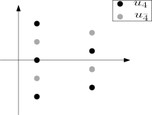
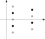
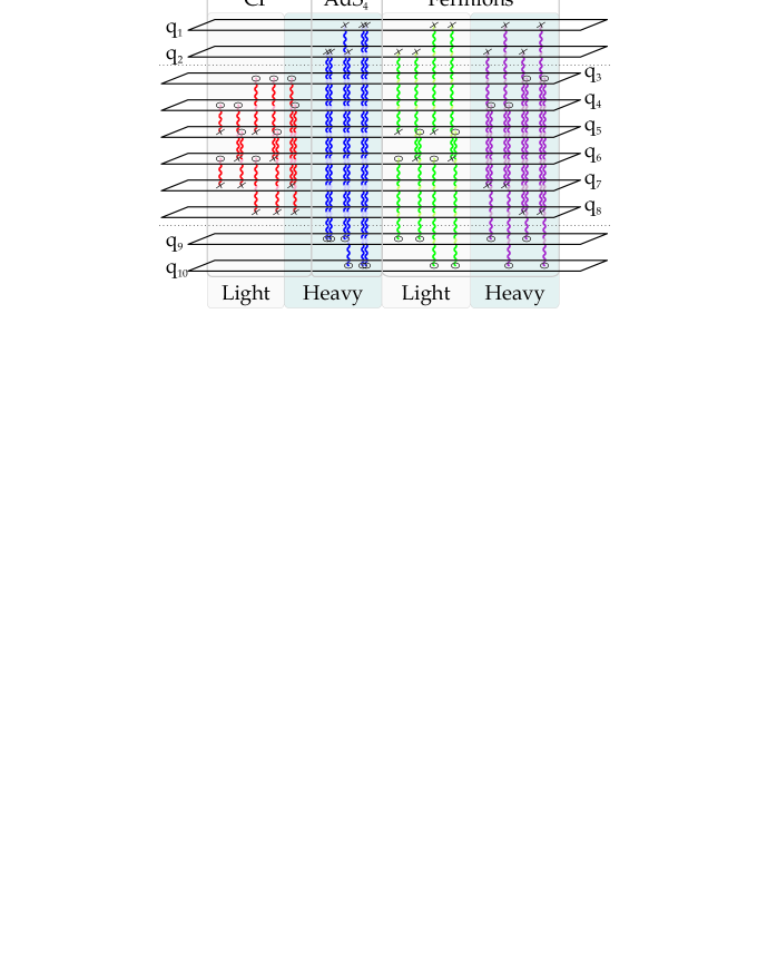
The pattern of excitations in the ABJM theory is quite different from that of ${\rm AdS}_{5}\times{\rm S}^{5}$. The string in ${\rm AdS}_{4}\times{\mathbb{CP}}^{3}$ has $8$ bosonic ($3$ modes of ${\rm AdS}_{4}$ and $5$ of ${\mathbb{CP}}^{3}$) and $8$ fermionic excitations. They are divided into heavy and light modes (see Fig.3). The dispersion relations for the heavy and light modes differ by a factor of two. We will see that this complicated structure of heavy and light fluctuations is captured by the Y-system. As usual the one-loop shift is given by a sum over the fluctuation energies [64]. In the algebraic curve language the fluctuations are the small cuts (i.e. poles) connecting different sheets of the algebraic curve $q_{i}$. The poles could be placed only in certain special positions $x_{n}^{ij}$ given by

$$q_{i}(x_{n}^{ij})-q_{j}(x_{n}^{ij})=2\pi n\;.$$ (5.1)

The quasiclassical Bohr-Sommerfeld quantization condition constrains the minimal residue of the pole. Insertion of the pole results in displacement of the other singularities. Moreover the pole by itself carries the energy $\omega(x_{n}^{ij})$ for the light mode and $2\omega(x_{n}^{ij})$ for the heavy mode where

$$\omega(x)=\frac{1}{x^{2}-1}.$$ (5.2)

Following [32] we first compute this second part of the one-loop shift which does not take into account the back-reaction of the fluctuation on the large cuts. Then we have

$$\delta E_{1-loop}^{0}=\frac{1}{2}\sum_{n}\sum_{\rm light}(-1)^{F_{ij}}\omega(x_{n}^{ij})+\sum_{n}\sum_{\rm heavy}(-1)^{F_{ij}}\omega(x_{n}^{ij})$$ (5.3)

where $F_{ij}=1$ for bosonic modes and $-1$ for fermionic. The modes are

$\displaystyle(i,j)$ $\displaystyle=$ $\displaystyle(4,5),(4,6),(3,5),(3,6)\;\;,\;\;{\rm light\;bosonic\;modes}$ (5.4)
$\displaystyle(i,j)$ $\displaystyle=$ $\displaystyle(3,7),(2,9),(1,9),(1,10)\;\;,\;\;{\rm heavy\;bosonic\;modes}$ (5.5)
$\displaystyle(i,j)$ $\displaystyle=$ $\displaystyle(2,5),(2,6),(1,5),(1,6)\;\;,\;\;{\rm light\;fermionic\;modes}$ (5.6)
$\displaystyle(i,j)$ $\displaystyle=$ $\displaystyle(2,7),(1,7),(2,8),(1,8)\;\;,\;\;{\rm heavy\;fermionic\;modes}$ (5.7)

Rewriting the sum (5.3) as an integral we get

$$\delta E_{1-loop}^{0}=\sum_{(ij)}{\begin{picture}(1.0,1.0)(8.67,-11.5)\end{picture}}\oint_{{\mathbb{U}}^{+}}\frac{dx}{2\pi i}\omega(x)\partial_{x}{\cal N}_{0}$$ (5.8)

where the integration goes over the upper half of the unit circle $|x|=1$ and we denote

$$e^{{\cal N}_{0}}=\prod_{\rm light}(1-e^{-ip_{i}+ip_{j}})^{F_{ij}}\prod_{\rm heavy}(1-e^{-ip_{i}+ip_{j}})^{2F_{ij}}$$ (5.9)

Note that $\partial_{x}{\cal N}_{0}$ is constructed to have the residue $\pm 1$ ($\pm 2$) exactly at the position of the light (heavy) mode $x_{n}^{ij}$. More explicitly we can write

$$e^{{\cal N}_{0}}=\frac{(\lambda_{1}^{2}-1)^{2}(\lambda_{2}^{2}-1)^{2}(\lambda_{1}\lambda_{2}-1)^{2}(\lambda_{3}\lambda_{4}-1)^{2}(\lambda_{3}-\lambda_{5})(\lambda_{4}-\lambda_{5})(\lambda_{3}\lambda_{5}-1)(\lambda_{4}\lambda_{5}-1)}{(\lambda_{1}\lambda_{3}-1)^{2}(\lambda_{2}\lambda_{3}-1)^{2}(\lambda_{1}\lambda_{4}-1)^{2}(\lambda_{2}\lambda_{4}-1)^{2}(\lambda_{1}-\lambda_{5})(\lambda_{2}-\lambda_{5})(\lambda_{1}\lambda_{5}-1)(\lambda_{2}\lambda_{5}-1)}$$ (5.10)

where

$$\lambda_{a}=e^{-iq_{a}}\;.$$ (5.11)

For $sl_{2}$ sector [12] there are only cuts connecting 2nd and 9th sheets so that

$$\lambda_{5}=1\;\;,\;\;\lambda_{3}=\lambda_{4}=\Delta\;\;,\;\;\lambda_{2}=\Delta f\;\;,\;\;\lambda_{2}=\Delta\bar{f}$$ (5.12)

and (5.10) simplifies to

$$e^{{\cal N}_{0}}=\frac{(\Delta-1)^{6}(\Delta+1)^{2}(\Delta f+1)^{2}(\Delta\bar{f}+1)^{2}(\Delta^{2}f\bar{f}-1)^{2}}{(\Delta^{2}f-1)^{4}(\Delta^{2}\bar{f}-1)^{4}}\;,$$ (5.13)

where we recognize ${\cal N}_{0}=-{\cal M}_{0}$ and (5.8) coincides precisely with the second term in (4.39)!

Then one should also take into account the back-reaction of the fluctuations. As it is explained in detail in [32] for that one should work with the modified Bethe equations. We need to consider only the fluctuations touching those sheets where the macroscopic cuts are located. Hence, one of those sheets has to be the 2nd or the 9th sheet. Computing the r.h.s of (5.9) with that restriction imposed, we get, similarly to [32],

$\displaystyle e^{{\cal N}_{+}}$ $\displaystyle=$ $\displaystyle-\frac{(\lambda_{1}\lambda_{2}-1)(\lambda_{2}^{2}-1){}^{2}}{(\lambda_{2}\lambda_{3}-1)(\lambda_{2}\lambda_{4}-1)(\lambda_{2}-\lambda_{5})(\lambda_{2}-1/\lambda_{5})}$ (5.14)
$\displaystyle e^{{\cal N}_{-}}$ $\displaystyle=$ $\displaystyle-\frac{(\lambda_{1}^{2}-1){}^{2}(\lambda_{1}\lambda_{2}-1)}{(\lambda_{1}\lambda_{3}-1)(\lambda_{1}\lambda_{4}-1)(\lambda_{1}-\lambda_{5})(\lambda_{1}-1/\lambda_{5})}$ (5.15)

and from (5.12) we get

$$e^{{\cal N}_{+}}=-\frac{(\Delta f+1)^{2}(\Delta^{2}f\bar{f}-1)}{(\Delta^{2}f-1)^{2}}\;\;,\;\;e^{{\cal N}_{-}}=-\frac{(\Delta\bar{f}+1)^{2}(\Delta^{2}f\bar{f}-1)}{(\Delta^{2}\bar{f}-1)^{2}}$$ (5.16)

and we recognize exactly the same structures (4.37) we got from solving the Y-system!

Finally by putting $\lambda_{2}=\lambda_{3}=\lambda_{4}=0$ we obtain

$$e^{{\cal N}_{0}}=\frac{(\lambda_{1}^{2}-1)^{2}\lambda_{5}}{(\lambda_{1}-\lambda_{5})(\lambda_{1}\lambda_{5}-1)}$$ (5.17)

which is again precisely the quantity $e^{-{\cal M}_{0}}$ obtained for this sector in (4.45)!

We see that the nontrivial pattern of the fluctuations is reflected in the Y-system thus providing a direct link with the worldsheet theory. This is also a deep test of the structure of the Y-system equations we proposed.

6 Conclusion

In this paper we refined the Y-system for the ABJM theory which was conjectured in [19]. We derived it directly through the TBA approach and then made several highly nontrivial tests at strong coupling. In particular we constructed the general $\mathfrak{sl}_{2}$ solution for the new Y-system in the scaling limit, and also made a test for a subsector where the difference between the old and the new Y-systems is crucial.

We also constructed the general asymptotic solution of the Y-system for arbitrary excited states. It can be used, in particular, for the weak coupling tests of the conjecture and as an initial configuration for numerical iterative solutions.

Note added While we were working on the strong coupling solution, the paper [65] appeared, with a similar Y-system and vacuum TBA equations.

Acknowledgments

The work of NG was partially supported by the German Science Foundation (DFG) under the Collaborative Research Center (SFB) 676 and RFFI project grant 06-02-16786. The work of F. L.-M. was partially supported by the Dynasty Foundation (Russia) and by the grant NS-5525.2010.2. We thank V.Kazakov, P.Vieira, V.Schomerus and Z.Tsuboi for discussions. NG is grateful to the Simons Center for Geometry And Physics, where a part of the work was done, for the kind hospitality. F. L.-M. thanks DESY, where a part of this work was done, for hospitality during the 2009 summer school.

Appendix A Notation and kernels

We use the following notation for kernels in TBA equations:

$\displaystyle K_{n}(u,v)$ $\displaystyle\equiv$ $\displaystyle\frac{1}{2\pi i}\frac{\partial}{\partial v}\ln\frac{u-v+in/2}{u-v-in/2},$ (A.1)
$\displaystyle K_{n,m}(u,v)$ $\displaystyle\equiv$ $\displaystyle\sum_{j=-\frac{m-1}{2}}^{\frac{m-1}{2}}\sum_{k=-\frac{n-1}{2}}^{\frac{n-1}{2}}K_{2j+2k+2}(u,v),$ (A.2)
$\displaystyle{\cal S}_{nm}(u,v)$ $\displaystyle\equiv$ $\displaystyle\frac{1}{2\pi i}\frac{\partial}{\partial v}\log\sigma_{BES}(x^{[+n]}(u),x^{[-n]}(u),x^{[+m]}(v),x^{[-m]}(v))$ (A.3)
$\displaystyle\tilde{\cal S}_{nm}(u,v)$ $\displaystyle\equiv$ $\displaystyle{\cal S}_{nm}(u,v)+\frac{ni}{2}{\cal P}^{(m)}(v)$ (A.4)
$\displaystyle\mathcal{B}^{(ab)}_{nm}(u,v)$ $\displaystyle\equiv$ $\displaystyle\sum_{j=-\frac{n-1}{2}}^{\frac{n-1}{2}}\sum_{k=-\frac{m-1}{2}}^{\frac{m-1}{2}}\frac{1}{2\pi i}\frac{\partial}{\partial v}\log\frac{b(u+ia/2+ij,v-ib/2+ik)}{b(u-ia/2+ij,v+ib/2+ik)}$ (A.5)
$\displaystyle\mathcal{R}^{(ab)}_{nm}(u,v)$ $\displaystyle\equiv$ $\displaystyle\sum_{j=-\frac{n-1}{2}}^{\frac{n-1}{2}}\sum_{k=-\frac{m-1}{2}}^{\frac{m-1}{2}}\frac{1}{2\pi i}\frac{\partial}{\partial v}\log\frac{r(u+ia/2+ij,v-ib/2+ik)}{r(u-ia/2+ij,v+ib/2+ik)},$ (A.6)

where

$$b(u,v)=\frac{1/x^{{\rm mir}}(u)-x^{{\rm mir}}(v)}{\sqrt{x^{{\rm mir}}(v)}},\ \ r(u,v)=\frac{x^{{\rm mir}}(u)-x^{{\rm mir}}(v)}{\sqrt{x^{{\rm mir}}(v)}},$$ (A.7)

and

$${\cal P}^{(a)}(v)=-\frac{1}{2\pi}\partial_{v}\log\frac{x^{{\rm mir}}(v+ia/2)}{x^{{\rm mir}}(v-ia/2)}\;.$$ (A.8)

To derive (3.43) we use the following integral representation [24, 25]:

$\displaystyle 2{\cal\tilde{S}}_{nm}(u,v)-{\cal R}_{nm}^{(11)}(u,v)+{\cal B}_{nm}^{(11)}(u,v)=-{K}_{n,m}(u-v)$ (A.9)
$\displaystyle-2\sum_{a=1}^{\infty}\int\left[{\cal B}^{(10)}_{n1}\left(u,w+ia/2\right){\cal B}_{1m}^{(01)}\left(w-ia/2,v\right)+{\cal B}^{(10)}_{n1}\left(u,w-ia/2\right){\cal B}_{1m}^{(01)}\left(w+ia/2,v\right)\right]dw.$

Equation (3.43) follows due to the identity ${\cal R}_{nm}^{(11)}(u,v)+{\cal B}_{nm}^{(11)}(u,v)={K}_{n,m}(u-v)$.

Appendix B Fermionic duality transformation and $\mathfrak{su}(2)$

We can transform a set of Bethe equations into an equivalent one by application of the fermionic duality. This follows [9] closely. We construct the polynomial

$\displaystyle P(x)$ $\displaystyle=$ $\displaystyle\prod_{j=1}^{K_{4}}(x-x_{4,j}^{+})\prod_{j=1}^{K_{\bar{4}}}(x-x_{\bar{4},j}^{+})\prod_{j=1}^{K_{2}}(x-x_{2,j}^{-})(x-1/x_{2,j}^{-})$ (B.1)
$\displaystyle-$ $\displaystyle\prod_{j=1}^{K_{4}}(x-x_{4,j}^{-})\prod_{j=1}^{K_{\bar{4}}}(x-x_{\bar{4},j}^{-})\prod_{j=1}^{K_{2}}(x-x_{2,j}^{+})(x-1/x_{2,j}^{+})$

from the Bethe equations of [12] (given in section 2.1 of the present work) for the fermionic roots $u_{1}$ and $u_{3}$. We see that this polynomial has zeros for $x=1/x_{1,j}$ and $x=x_{3,j}$. Denoting the remaining zeros of this polynomial by $\tilde{x}$, we get

$$P(x)=C\prod_{j=1}^{K_{3}}(x-x_{3,j})\prod_{j=1}^{K_{1}}(x-1/x_{1,j})\prod_{j=1}^{\tilde{K}_{3}}(x-\tilde{x}_{3,j})\prod_{j=1}^{\tilde{K}_{1}}(x-1/\tilde{x}_{1,j})$$ (B.2)

(where $C$ is a constant) or in our notation (with $R\equiv R_{4}R_{\bar{4}},\ B\equiv B_{4}B_{\bar{4}}$)

$$P(x)=CR_{3}B_{1}R_{\tilde{3}}B_{\tilde{1}}=\left[R^{(-)}Q_{2}^{+}-R^{(+)}Q_{2}^{-}\right]\left(\frac{x}{h}\right)^{K_{2}}\prod_{j=1}^{K_{4}}\sqrt{x_{4,j}^{+}}$$ (B.3)
$$\frac{P(x^{+})}{P(x^{-})}=\frac{R^{+}_{3}B^{+}_{1}R^{+}_{\tilde{3}}B^{+}_{\tilde{1}}}{R^{-}_{3}B^{-}_{1}R^{-}_{\tilde{3}}B^{-}_{\tilde{1}}}=\left(\frac{x^{+}}{x^{-}}\right)^{K_{2}}\frac{R^{(-)+}Q_{2}^{++}-R^{(+)+}Q_{2}}{R^{(-)-}Q_{2}-R^{(+)-}Q_{2}^{--}}$$ (B.4)

and

$$\frac{P(1/x^{-})}{P(1/x^{+})}=\frac{B^{-}_{3}R^{-}_{1}B^{-}_{\tilde{3}}R^{-}_{\tilde{1}}}{B^{+}_{3}R^{+}_{1}B^{+}_{\tilde{3}}R^{+}_{\tilde{1}}}=\left(\frac{x^{+}}{x^{-}}\right)^{K_{2}}\frac{B^{(-)-}Q_{2}-B^{(+)-}Q_{2}^{--}}{B^{(-)+}Q_{2}^{++}-B^{(+)+}Q_{2}}$$ (B.5)

then

$$f(u)=-\left(\frac{x^{+}}{x^{-}}\right)^{K_{2}}\frac{R^{(+)+}B_{1}^{-}\tilde{B}_{1}^{-}B_{3}^{+}\tilde{B}_{3}^{+}}{R^{(-)-}B_{1}^{+}\tilde{B}_{1}^{+}B_{3}^{-}\tilde{B}_{3}^{-}}\;\;,\;\;f_{a}(u)\equiv\prod_{n=-\frac{a-1}{2}}^{\frac{a-1}{2}}f(u+in)$$ (B.6)
$\displaystyle T_{a,1}(u|\{u_{1,j}\},\{u_{3,j}\})$ $\displaystyle=$ $\displaystyle f_{a}(u)\overline{T_{1,a}(u|\{\tilde{u}_{1,j}\},\{\tilde{u}_{3,j}\})}$ (B.7)
$\displaystyle T_{1,s}(u|\{u_{1,j}\},\{u_{3,j}\})$ $\displaystyle=$ $\displaystyle f_{s}(u)\overline{T_{s,1}(u|\{\tilde{u}_{1,j}\},\{\tilde{u}_{3,j}\})}$ (B.8)

Here, the bar means complex conjugation in the physical sense, i.e. the replacement

$$R^{(\pm)\pm}\to R^{(\mp)\mp}\;\;,\;\;B^{(\pm)\pm}\to B^{(\mp)\mp}.$$ (B.9)

Notice that $x$ is not inverting under this conjugation.

𝐘a(x[a]x[+a])LK2𝐓a,1¯n=a12a12Φ~4θnaE(u+in)Φ~4¯θnaO(u+in),similar-to-or-equalssubscript𝐘subscript𝑎superscriptsuperscript𝑥delimited-[]𝑎superscript𝑥delimited-[]𝑎𝐿subscript𝐾2¯subscript𝐓𝑎1superscriptsubscriptproduct𝑛𝑎12𝑎12superscriptsubscript~Φ4subscriptsuperscript𝜃E𝑛𝑎𝑢𝑖𝑛superscriptsubscript~Φ¯4subscriptsuperscript𝜃O𝑛𝑎𝑢𝑖𝑛\displaystyle{\bf Y}_{\scalebox{0.67}{\begin{picture}(5.21,0.0)\put(-1.5,1.2){$\blacktriangleleft$}\end{picture}}_{a}}\simeq\left(\frac{x^{[-a]}}{x^{[+a]}}\right)^{L-K_{2}}\overline{{\bf T}_{a,1}}\prod_{n=-\frac{a-1}{2}}^{\frac{a-1}{2}}\tilde{\Phi}_{4}^{\theta^{\rm E}_{na}}(u+in)\tilde{\Phi}_{\bar{4}}^{\theta^{\rm O}_{na}}(u+in), (B.10)
𝐘a(x[a]x[+a])LK2𝐓a,1¯n=a12a12Φ~4θnaO(u+in)Φ~4¯θnaE(u+in)similar-to-or-equalssubscript𝐘subscript𝑎superscriptsuperscript𝑥delimited-[]𝑎superscript𝑥delimited-[]𝑎𝐿subscript𝐾2¯subscript𝐓𝑎1superscriptsubscriptproduct𝑛𝑎12𝑎12superscriptsubscript~Φ4subscriptsuperscript𝜃O𝑛𝑎𝑢𝑖𝑛superscriptsubscript~Φ¯4subscriptsuperscript𝜃E𝑛𝑎𝑢𝑖𝑛\displaystyle{\bf Y}_{\scalebox{0.67}{\begin{picture}(5.21,0.0)\put(-1.5,1.2){$\blacktriangleright$}\end{picture}}_{a}}\simeq\left(\frac{x^{[-a]}}{x^{[+a]}}\right)^{L-K_{2}}\overline{{\bf T}_{a,1}}\prod_{n=-\frac{a-1}{2}}^{\frac{a-1}{2}}\tilde{\Phi}_{4}^{\theta^{\rm O}_{na}}(u+in)\tilde{\Phi}_{\bar{4}}^{\theta^{\rm E}_{na}}(u+in) (B.11)

As in section 2, the factors Φ~4(u)subscript~Φ4𝑢\tilde{\Phi}_{4}(u) and Φ~4¯(u)subscript~Φ¯4𝑢\tilde{\Phi}_{\bar{4}}(u) are constructed in such a way that the ABA equations for the momentum carrying nodes are given by 𝐘1ph(u4,j)=1superscriptsubscript𝐘subscript1phsubscript𝑢4𝑗1{\bf Y}_{\scalebox{0.67}{\begin{picture}(5.21,0.0)\put(-1.5,1.2){$\blacktriangleleft$}\end{picture}}_{1}}^{{\rm ph}}(u_{4,j})=-1 and 𝐘1ph(u4¯,j)=1superscriptsubscript𝐘subscript1phsubscript𝑢¯4𝑗1{\bf Y}_{\scalebox{0.67}{\begin{picture}(5.21,0.0)\put(-1.5,1.2){$\blacktriangleright$}\end{picture}}_{1}}^{{\rm ph}}(u_{\bar{4},j})=-1. We have

$$\tilde{\Phi}_{4}(u)=-S_{4}S_{\bar{4}}\frac{B_{4}^{(+)+}R_{4}^{(-)-}\tilde{B}_{1}^{-}\tilde{B}_{3}^{+}}{B_{4}^{(-)-}R_{4}^{(+)+}\tilde{B}_{1}^{+}\tilde{B}_{3}^{-}}e^{i{\cal Q}_{1}/2}\;\;,\;\;\tilde{\Phi}_{\bar{4}}(u)=-S_{4}S_{\bar{4}}\frac{B_{\bar{4}}^{(+)+}R_{\bar{4}}^{(-)-}\tilde{B}_{1}^{-}\tilde{B}_{3}^{+}}{B_{\bar{4}}^{(-)-}R_{\bar{4}}^{(+)+}\tilde{B}_{1}^{+}\tilde{B}_{3}^{-}}e^{i{\cal Q}_{1}/2}\;.$$ (B.12)

where $\tilde{B}_{l},\tilde{R}_{l}$ are defined similarly to (2.8), (2.9), with $x_{l,j}$ replaced by $\tilde{x}_{l,j}$.

Appendix C Explicit expressions for Y-functions

Here we present the solution of the Y-system in the scaling limit for the sl(2)𝑠𝑙2sl(2) sector. This solution was obtained in section 4, and below we give its explicit form, which can be used in the Mathematica system. We denote 𝚍=Δ,𝚐=f4,𝚐𝚋=f¯4,Ym[a_]=Ya,Yp[a_]=Ya,Yb[s_]=Ysformulae-sequence𝚍Δformulae-sequence𝚐subscript𝑓4formulae-sequence𝚐𝚋subscript¯𝑓4formulae-sequencemonospace-Ym[a_]subscript𝑌subscript𝑎formulae-sequencemonospace-Yp[a_]subscript𝑌subscript𝑎monospace-Yb[s_]subscript𝑌subscript𝑠\verb"d"=\Delta,\;\verb"g"=f_{4},\;\verb"gb"=\bar{f}_{4},\;\verb"Ym[a_]"=Y_{\scalebox{1.15}{\begin{picture}(2.8,0.0)\put(-1.2,-0.33){$\bullet$}\end{picture}}_{a}},\;\verb"Yp[a_]"=Y_{\scalebox{0.6}[0.7]{\begin{picture}(7.24,0.2)\put(-1.5,0.5){$\bigtriangleup$}\end{picture}}_{a}},\;\verb"Yb[s_]"=Y_{\scalebox{0.5}{\begin{picture}(7.27,0.3)\put(-1.7,2.65){$\bigcirc$}\end{picture}}_{s}}, and the Y-functions are given by the following code:


sb={
A-> ((1+d)(1-d g^2-g gb+2 d g gb-d^2 g gb-d gb^2+d^2 g^2 gb^2)
(1-d g^2+g gb-2 d g gb+d^2 g gb-d gb^2+d^2 g^2 gb^2))/
((-1+d)(-1+g)(1+g)(-1+d g)(1+d g)(-1+gb)(1+gb)(-1+d gb)(1+d gb)),
S1->((-1+g)(1+g)gb^2(-1+d gb)(1+d gb))/(g^2(-1+d g)(1+d g)(-1+gb)(1+gb)),
S2->((-1+g)(1+g)(-1+gb)(1+gb))/(g^2(-1+d g)(1+d g)gb^2(-1+d gb)(1+d gb)),
P-> ((-1+d g^2)^2(-1+d gb^2)^2)/((-1+d)^4g^2gb^2),
T2->d g gb, T1->-(g/gb)};

Ym[a_]=-1+(S2 T2^(1+a)(-1+T2^2)-S1^2 S2 T1^(4+2a)T2^(1+a)(-1+T2^2)+
S1 T1^(1+a)(-1+T1^2)(-1+S2^2 T2^(4+2a)))^2/
((-S2 T2^a (-1+T2^2)+S1^2 S2 T1^(2+2 a)T2^a (-1+T2^2)-
S1 T1^a (-1+T1^2)(-1+S2^2 T2^(2+2 a)))(-S2 T2^(2+a)(-1+T2^2)+
S1^2 S2 T1^(6+2 a) T2^(2+a)(-1+T2^2)-
S1 T1^(2+a)(-1+T1^2)(-1+S2^2 T2^(6+2 a))))/.sb;

Yp[a_]=((S1 T1^(4+a) T2)/(-1+T1^2)+(T1^-a T2)/(S1-S1 T1^2)-
(T1(T2^-a-S2^2 T2^(4+a)))/(S2 - S2 T2^2))^2/(-((S1 T1^(4+a)T2)/
(-1+T1^2)+(T1^-a T2)/(S1 - S1 T1^2)-(T1(T2^-a-S2^2 T2^(4+a)))/
(S2-S2 T2^2))^2+(T1^(-2 a)T2^(-2 a)(T2^2-S2^2 T2^(4+2 a)-
2 S1 S2 T1^(2+a)T2^(2+a)(-1+T2^2)+2 S1 S2 T1^(4+a)T2^(2+a)(-1+T2^2)+
S1^2 T1^(6+2 a)T2^2(-1+S2^2 T2^(2+2 a))+2 T1 T2 (-1+S2^2 T2^(4+2 a))-
2 S1^2 T1^(5+2 a)T2(-1+S2^2 T2^(4+2 a))+T1^2 (1-S2^2 T2^(6+2 a))+
S1^2 T1^(4+2 a)(-1+S2^2 T2^(6+2 a)))^2)/(S1^2 S2^2 (-1+T1^2)^2
(-1+T2^2)^2(T2+T1^2 T2-T1(1+T2^2))^2))/.sb;

Yb[s_]=(s-A)^2-1/.sb;

Y11=(-1+(S1 S2(-1+T1^2)(-1+T2^2)(T2^2-S2^2 T2^6-2 S1 S2 T1^3 T2^3 (-1+T2^2)+
2 S1 S2 T1^5 T2^3(-1+T2^2)+S1^2 T1^8 T2^2(-1+S2^2 T2^4)+
2 T1 T2(-1+S2^2 T2^6)-2 S1^2 T1^7 T2(-1+S2^2 T2^6)+T1^2 (1-S2^2 T2^8)+
S1^2 T1^6 (-1+S2^2 T2^8))^2)/((S1^2 S2 T1^4 T2 (-1+T2^2)+S2 (T2-T2^3)-
S1 T1 (-1+T1^2)(-1+S2^2 T2^4))^2 (T2^2-S2^2 T2^8-2 S1 S2 T1^4 T2^4 (-1+T2^2)+
2 S1 S2 T1^6 T2^4 (-1+T2^2)+S1^2 T1^10 T2^2 (-1+S2^2 T2^6)+2 T1 T2 (-1+S2^2 T2^8)-
2 S1^2 T1^9 T2 (-1+S2^2 T2^8)+T1^2 (1-S2^2 T2^10)+S1^2 T1^8 (-1+S2^2 T2^10))))/.sb;

Y22=(P/Y11)/.sb;

References

  • [1] J. M. Maldacena, “The large N limit of superconformal field theories and supergravity”, Adv. Theor. Math. Phys.  2 (1998) 231 [Int. J. Theor. Phys.  38 (1999) 1113] [arXiv:hep-th/9711200].
  • [2] O. Aharony, O. Bergman, D. L. Jafferis and J. Maldacena, “N=6 superconformal Chern-Simons-matter theories, M2-branes and their gravity duals”, JHEP 0810, 091 (2008) [arXiv:0806.1218 [hep-th]] $::\clubsuit::$ O. Aharony, O. Bergman and D. L. Jafferis, “Fractional M2-branes”, JHEP 0811, 043 (2008) [arXiv:0807.4924 [hep-th]].
  • [3] J. A. Minahan and K. Zarembo, “The Bethe-ansatz for N = 4 super Yang-Mills”, JHEP 0303 (2003) 013 [arXiv:hep-th/0212208] $::\clubsuit::$ J.A. Minahan and K. Zarembo, “The Bethe ansatz for superconformal Chern-Simons”, JHEP 0809, 040 (2008) [arXiv:0806.3951] $::\clubsuit::$ D. Gaiotto, S. Giombi and X. Yin, “Spin Chains in ${\cal N}=6$ Superconformal Chern-Simons-Matter Theory”, JHEP 0904, 066 (2009) [arXiv:0806.4589] $::\clubsuit::$ D. Bak and S.J. Rey, “Integrable Spin Chain in Superconformal Chern-Simons Theory”, JHEP 0810, 053 (2008) [arXiv:0807.2063] $::\clubsuit::$ C. Kristjansen, M. Orselli and K. Zoubos, “Non-planar ABJM theory and integrability”, JHEP 0903, 037 (2009) [arXiv:0811.2150] $::\clubsuit::$ B.I. Zwiebel, “Two-loop Integrability of Planar ${\cal N}=6$ Superconformal Chern-Simons Theory”, [arXiv:0901.0411] $::\clubsuit::$ J.A. Minahan, W. Schulgin and K. Zarembo, “Two loop integrability for Chern-Simons theories with ${\cal N}=6$ supersymmetry”, JHEP 0903, 057 (2009) [arXiv:0901.1142] $::\clubsuit::$ D. Bak, H. Min and S.J. Rey, “Generalized Dynamical Spin Chain and 4-Loop Integrability in ${\cal N}=6$ Superconformal Chern-Simons Theory”, [arXiv:0904.4677] $::\clubsuit::$ B. Chen and J. B. Wu, “Semi-classical strings in $AdS_{4}\times CP^{3}$, JHEP 0809, 096 (2008) [arXiv:0807.0802 [hep-th]].
  • [4] J.A. Minahan, O.O. Sax and C. Sieg, “Magnon dispersion to four loops in the ABJM and ABJ models”, [arXiv:0908.2463]. $::\clubsuit::$ J. A. Minahan, O. O. Sax and C. Sieg, “Anomalous dimensions at four loops in N=6 superconformal Chern-Simons theories”, arXiv:0912.3460.
  • [5] I. Bena, J. Polchinski and R. Roiban, “Hidden symmetries of the AdS$(5)\times{\rm S}^{5}$ superstring”, Phys. Rev.  D 69 (2004) 046002 [arXiv:hep-th/0305116].
  • [6] B.J. Stefanski, “Green-Schwarz action for Type IIA strings on ${\rm AdS}_{4}\times{\mathbb{CP}}^{3}$, Nucl. Phys.  B 808, 80 (2009) [arXiv:0806.4948] $::\clubsuit::$ G. Arutyunov and S. Frolov, “Superstrings on ${\rm AdS}_{4}\times{\mathbb{CP}}^{3}$ as a Coset Sigma-model”, JHEP 0809, 129 (2008) [arXiv:0806.4940] $::\clubsuit::$ J. Gomis, D. Sorokin and L. Wulff, “The complete ${\rm AdS}_{4}\times{\mathbb{CP}}^{3}$ superspace for the type IIA superstring and D-branes”, JHEP 0903, 015 (2009) [arXiv:0811.1566] $::\clubsuit::$ D. Astolfi, V. G. M. Puletti, G. Grignani, T. Harmark and M. Orselli, “Finite-size corrections in the $SU(2)\times SU(2)$ sector of type IIA string theory on ${\rm AdS}_{4}\times{\mathbb{CP}}^{3}$, Nucl. Phys. B810, 150 (2009) [arXiv:0807.1527] $::\clubsuit::$ P. Sundin, “The ${\rm AdS}_{4}\times CP_{3}$ string and its Bethe equations in the near plane wave limit”, JHEP 0902, 046 (2009) [arXiv:0811.2775] $::\clubsuit::$ P. Sundin, “On the worldsheet theory of the type IIA ${\rm AdS}_{4}\times CP_{3}$ superstring”, [arXiv:0909.0697] $::\clubsuit::$ K. Zarembo, “Worldsheet spectrum in ${\rm AdS}_{4}/{\rm CFT}_{3}$ correspondence”, JHEP 0904, 135 (2009) [arXiv:0903.1747] $::\clubsuit::$ C. Kalousios, C. Vergu and A. Volovich, “Factorized Tree-level Scattering in ${\rm AdS}_{4}\times{\mathbb{CP}}^{3}$, [arXiv:0905.4702].
  • [7] M. Staudacher, “The factorized $S$-matrix of CFT/AdS”, JHEP 0505, 054 (2005) [arXiv:hep-th/0412188] $::\clubsuit::$ N. Beisert, “The $su(2|2)$ dynamic $S$-matrix”, Adv. Theor. Math. Phys. 12, 945 (2008) [arXiv:hep-th/0511082] $::\clubsuit::$ N. Beisert, “The Analytic Bethe Ansatz for a Chain with Centrally Extended $su(2|2)$ Symmetry”, J. Stat. Mech. 0701, P017 (2007) [arXiv:nlin/0610017] $::\clubsuit::$ R.A. Janik, “The ${\rm AdS}_{5}\times{\rm S}^{5}$ superstring worldsheet $S$-matrix and crossing symmetry”, Phys. Rev. D73, 086006 (2006) [arXiv:hep-th/0603038] $::\clubsuit::$ N. Beisert, R. Hernandez and E. Lopez, “A crossing-symmetric phase for ${\rm AdS}_{5}\times{\rm S}^{5}$ strings”, JHEP 0611, 070 (2006) [arXiv:hep-th/0609044]
  • [8] V.A. Kazakov, A. Marshakov, J.A. Minahan and K. Zarembo, “Classical / quantum integrability in AdS/CFT”, JHEP 0405, 024 (2004) [arXiv:hep-th/0402207] $::\clubsuit::$ V.A. Kazakov and K. Zarembo, “Classical / quantum integrability in non-compact sector of AdS/CFT”, JHEP 0410, 060 (2004) [arXiv:hep-th/0410105] $::\clubsuit::$ N. Beisert, V.A. Kazakov and K. Sakai, “Algebraic curve for the $SO(6)$ sector of AdS/CFT”, Commun. Math. Phys. 263, 611 (2006) [arXiv:hep-th/0410253] $::\clubsuit::$ S. Schäfer-Nameki, “The algebraic curve of 1-loop planar ${\cal N}=4$ SYM”, Nucl. Phys.  B 714, 3 (2005) [arXiv:hep-th/0412254] $::\clubsuit::$ N. Beisert, V.A. Kazakov, K. Sakai and K. Zarembo, “The algebraic curve of classical superstrings on ${\rm AdS}_{5}\times S^{5}$, Commun. Math. Phys. 263, 659 (2006) [arXiv:hep-th/0502226].
  • [9] N. Beisert and M. Staudacher, “Long-range PSU$(2,2|4)$ Bethe ansaetze for gauge theory and strings”, Nucl. Phys.  B 727 (2005) 1 [arXiv:hep-th/0504190]
  • [10] N. Beisert, B. Eden and M. Staudacher, “Transcendentality and crossing”, J. Stat. Mech. 0701, P021 (2007) [arXiv:hep-th/0610251].
  • [11] N. Gromov and P. Vieira, “The ${\rm AdS}_{4}/{\rm CFT}_{3}$ algebraic curve”, JHEP 0902, 040 (2009) [arXiv:0807.0437].
  • [12] N. Gromov and P. Vieira, “The all loop ${\rm AdS}_{4}/{\rm CFT}_{3}$ Bethe ansatz”, JHEP 0901, 016 (2009) [arXiv:0807.0777].
  • [13] C. Ahn and R.I. Nepomechie, ${\cal N}=6$ super Chern-Simons theory $S$-matrix and all-loop Bethe ansatz equations”, JHEP 0809, 010 (2008) [arXiv:0807.1924].
  • [14] A. Babichenko, B. Stefanski and K. Zarembo, “Integrability and the AdS(3)/CFT(2) correspondence”, arXiv:0912.1723.
  • [15] J. Ambjorn, R. A. Janik and C. Kristjansen, “Wrapping interactions and a new source of corrections to the spin-chain / string duality”, Nucl. Phys.  B 736 (2006) 288 [arXiv:hep-th/0510171].
  • [16] R. A. Janik and T. Lukowski, “Wrapping interactions at strong coupling – the giant magnon”, Phys. Rev.  D 76, 126008 (2007) [arXiv:0708.2208 [hep-th]]. $::\clubsuit::$ M. P. Heller, R. A. Janik and T. Lukowski, “A new derivation of Luscher F-term and fluctuations around the giant magnon”, JHEP 0806, 036 (2008) [arXiv:0801.4463 [hep-th]].
  • [17] Z. Bajnok and R. A. Janik, “Four-loop perturbative Konishi from strings and finite size effects for multiparticle states”, Nucl. Phys.  B 807, 625 (2009) [arXiv:0807.0399].
  • [18] C. N. Yang and C. P. Yang, “One-dimensional chain of anisotropic spin-spin interactions. I: Proof of Bethe’s hypothesis for ground state in a finite system”, Phys. Rev.  150 (1966) 321 $::\clubsuit::$ A. B. Zamolodchikov, “On the thermodynamic Bethe ansatz equations for reflectionless ADE scattering theories”, Phys. Lett.  B 253, 391 (1991) $::\clubsuit::$ N. Dorey, “Magnon bound states and the AdS/CFT correspondence”, J. Phys. A 39, 13119 (2006) [arXiv:hep-th/0604175] $::\clubsuit::$ M. Takahashi, “Thermodynamics of one-dimensional solvable models”, Cambridge University Press, 1999 $::\clubsuit::$ F.H.L. Essler, H.Frahm, F.Göhmann, A. Klümper and V. Korepin, “The One-Dimensional Hubbard Model”, Cambridge University Press, 2005 $::\clubsuit::$ V. V. Bazhanov, S. L. Lukyanov and A. B. Zamolodchikov, “Quantum field theories in finite volume: Excited state energies”, Nucl. Phys.  B 489, 487 (1997) [arXiv:hep-th/9607099] $::\clubsuit::$ P. Dorey and R. Tateo, “Excited states by analytic continuation of TBA equations,” Nucl. Phys.  B 482, 639 (1996) [arXiv:hep-th/9607167] $::\clubsuit::$ D. Fioravanti, A. Mariottini, E. Quattrini and F. Ravanini, “Excited state Destri-De Vega equation for sine-Gordon and restricted sine-Gordon models,” Phys. Lett.  B 390, 243 (1997) [arXiv:hep-th/9608091] $::\clubsuit::$ A. G. Bytsko and J. Teschner, “Quantization of models with non-compact quantum group symmetry: Modular XXZ magnet and lattice sinh-Gordon model,” J. Phys. A 39 (2006) 12927 [arXiv:hep-th/0602093] $::\clubsuit::$ N. Gromov, V. Kazakov and P. Vieira, “Finite Volume Spectrum of 2D Field Theories from Hirota Dynamics,” arXiv:0812.5091 [hep-th].
  • [19] N. Gromov, V. Kazakov and P. Vieira, “Exact Spectrum Of Anomalous Dimensions Of Planar N=4 Supersymmetric Yang-Mills Theory,” Phys. Rev. Lett.  103, 131601 (2009). [arXiv:0901.3753].
  • [20] F. Fiamberti, A. Santambrogio, C. Sieg and D. Zanon, “Anomalous dimension with wrapping at four loops in N=4 SYM,” Nucl. Phys.  B 805, 231 (2008) [arXiv:0806.2095] $::\clubsuit::$ V. N. Velizhanin, “Leading transcedentality contributions to the four-loop universal anomalous dimension in N=4 SYM,” arXiv:0811.0607.
  • [21] G. Arutyunov and S. Frolov, “On String S-matrix, Bound States and TBA,” JHEP 0712 (2007) 024 [arXiv:0710.1568 [hep-th]].
  • [22] F. Fiamberti, A. Santambrogio and C. Sieg, “Five-loop anomalous dimension at critical wrapping order in N=4 SYM,” arXiv:0908.0234 .
  • [23] D. Bombardelli, D. Fioravanti and R. Tateo, “Thermodynamic Bethe Ansatz for planar AdS/CFT: a proposal,” J. Phys. A 42, 375401 (2009) [arXiv:0902.3930]
  • [24] N. Gromov, V. Kazakov, A. Kozak and P. Vieira, “Integrability for the Full Spectrum of Planar AdS/CFT II,” arXiv:0902.4458 .
  • [25] G. Arutyunov and S. Frolov, “The Dressing Factor and Crossing Equations,” J. Phys. A 42 (2009) 425401 [arXiv:0904.4575 [hep-th]].
  • [26] G. Arutyunov and S. Frolov, “Thermodynamic Bethe Ansatz for the ${\rm AdS}_{5}\times{\rm S}^{5}$ Mirror Model,” JHEP 0905, 068 (2009) [arXiv:0903.0141].
  • [27] S. Frolov and R. Suzuki, “Temperature quantization from the TBA equations,” Phys. Lett.  B 679 (2009) 60 [arXiv:0906.0499 [hep-th]].
  • [28] G. Arutyunov and S. Frolov, “String hypothesis for the AdS5 x S5 mirror,” JHEP 0903 (2009) 152 [arXiv:0901.1417 [hep-th]].
  • [29] N. Gromov, V. Kazakov and P. Vieira, “Exact AdS/CFT spectrum: Konishi dimension at any coupling,” arXiv:0906.4240 .
  • [30] K. Konishi, “Anomalous Supersymmetry Transformation Of Some Composite Operators In Sqcd,” Phys. Lett.  B 135, 439 (1984). $::\clubsuit::$ M. Bianchi, S. Kovacs, G. Rossi and Y. S. Stanev, “Properties of the Konishi multiplet in N = 4 SYM theory,” JHEP 0105 (2001) 042 [arXiv:hep-th/0104016] $::\clubsuit::$ B. Eden, C. Jarczak, E. Sokatchev and Y. S. Stanev, “Operator mixing in N = 4 SYM: The Konishi anomaly revisited,” Nucl. Phys.  B 722, 119 (2005) [arXiv:hep-th/0501077].
  • [31] S. S. Gubser, I. R. Klebanov and A. M. Polyakov, “Gauge theory correlators from non-critical string theory,” Phys. Lett.  B 428 (1998) 105
  • [32] N. Gromov, “Y-system and Quasi-Classical Strings,” arXiv:0910.3608.
  • [33] G. Arutyunov and S. Frolov, “Uniform light-cone gauge for strings in AdS(5) x S**5: Solving $su(1|1)$ sector,” JHEP 0601 (2006) 055 [arXiv:hep-th/0510208].
  • [34] R. Roiban and A. A. Tseytlin, “Quantum strings in $AdS_{5}\times S^{5}$: strong-coupling corrections to dimension of Konishi operator,” arXiv:0906.4294 $::\clubsuit::$ A. A. Tseytlin, “Quantum strings in $AdS_{5}\times S^{5}$ and AdS/CFT duality,” arXiv:0907.3238 .
  • [35] D. Bombardelli and D. Fioravanti, “Finite-Size Corrections of the $\mathbb{CP}^{3}$ Giant Magnons: the Lüscher terms”, JHEP 0907 (2009) 034 [arXiv:0810.0704].
  • [36] I. Shenderovich, “Giant magnons in ${\rm AdS}_{4}/{\rm CFT}_{3}$: dispersion, quantization and finite–size corrections”, [arXiv:0807.2861].
  • [37] N. Berkovits, “Super-Poincare covariant quantization of the superstring,” JHEP 0004 (2000) 018 [arXiv:hep-th/0001035].
  • [38] N. Gromov, V. Kazakov and P. Vieira, “Finite Volume Spectrum of 2D Field Theories from Hirota Dynamics,” arXiv:0812.5091 [hep-th].
  • [39] O. Bergman and S. Hirano, “Anomalous radius shift in AdS(4)/CFT(3),” JHEP 0907 (2009) 016 [arXiv:0902.1743 [hep-th]].
  • [40] L. Mazzucato and B. C. Vallilo, “On the Non-renormalization of the AdS Radius,” JHEP 0909 (2009) 056 [arXiv:0906.4572 [hep-th]] $::\clubsuit::$ G. Bonelli, P. A. Grassi and H. Safaai, “Exploring Pure Spinor String Theory on $AdS_{4}\times\mathbb{CP}^{3}$,” JHEP 0810 (2008) 085 [arXiv:0808.1051 [hep-th]].
  • [41] N. Beisert, J. A. Minahan, M. Staudacher and K. Zarembo, “Stringing spins and spinning strings,” JHEP 0309 (2003) 010 [arXiv:hep-th/0306139].
  • [42] Z. Tsuboi, “Analytic Bethe ansatz and functional equations for Lie superalgebra $sl(r+1|s+1)$,” J. Phys. A 30, 7975 (1997) $::\clubsuit::$ N. Beisert, “The Analytic Bethe Ansatz for a Chain with Centrally Extended $su(2|2)$ Symmetry,” J. Stat. Mech.  0701 (2007) P017 [arXiv:nlin/0610017].
  • [43] V. Kazakov, A. S. Sorin and A. Zabrodin, “Supersymmetric Bethe ansatz and Baxter equations from discrete Hirota dynamics,” Nucl. Phys.  B 790, 345 (2008) [arXiv:hep-th/0703147].
  • [44] H. Saleur and B. Pozsgay, “Scattering and duality in the 2 dimensional $OSP(2|2)$ Gross Neveu and sigma models,” arXiv:0910.0637.
  • [45] B. Vicedo, “Finite-g strings”, Cambridge PhD thesis (2008) [arXiv:0810.3402].
  • [46] T. Lukowski and O.O. Sax, “Finite size giant magnons in the $SU(2)\times SU(2)$ sector of ${\rm AdS}_{4}\times{\mathbb{CP}}^{3}$, JHEP 0812, 073 (2008) [arXiv:0810.1246].
  • [47] A.B. Zamolodchikov and Al.B. Zamolodchikov, “Factorized $S$ matrices in two-dimensions as the exact solutions of certain relativistic quantum field models”, Ann. Phys. 120, 253 (1979). $::\clubsuit::$ P. Dorey, “Exact S-matrices”, in Conformal field theories and integrable models, Z. Horváth and L. Palla eds. (Springer, 1997) [arXiv:hep-th/9810026].
  • [48] N. Beisert, C. Kristjansen and M. Staudacher, “The dilatation operator of N = 4 super Yang-Mills theory”, Nucl. Phys.  B 664 (2003) 131 [arXiv:hep-th/0303060].
  • [49] N. Beisert and M. Staudacher, “The N = 4 SYM integrable super spin chain”, Nucl. Phys.  B 670 (2003) 439 [arXiv:hep-th/0307042].
  • [50] N. Beisert, “The $su(2|3)$ dynamic spin chain”, Nucl. Phys.  B 682, 487 (2004) [arXiv:hep-th/0310252].
  • [51] M. Staudacher, “The factorized S-matrix of CFT/AdS”, JHEP 0505 (2005) 054 [arXiv:hep-th/0412188].
  • [52] N. Beisert, R. Hernandez and E. Lopez, “A crossing-symmetric phase for AdS$(5)\times{\rm S}^{5}$ strings”, JHEP 0611, 070 (2006) [arXiv:hep-th/0609044]; $::\clubsuit::$ N. Beisert, B. Eden and M. Staudacher, “Transcendentality and crossing”, J. Stat. Mech.  0701, P021 (2007) [arXiv:hep-th/0610251].
  • [53] V. V. Bazhanov, S. L. Lukyanov and A. B. Zamolodchikov, “Quantum field theories in finite volume: Excited state energies,” Nucl. Phys.  B 489 (1997) 487 [arXiv:hep-th/9607099].
  • [54] P. Dorey and R. Tateo, “Excited states by analytic continuation of TBA equations,” Nucl. Phys.  B 482 (1996) 639 [arXiv:hep-th/9607167].
  • [55] P. Dorey and R. Tateo, Nucl. Phys.  B 515 (1998) 575 [arXiv:hep-th/9706140].
  • [56] B. I. Zwiebel, “Two-loop Integrability of Planar N=6 Superconformal Chern-Simons Theory”, arXiv:0901.0411 [hep-th] $::\clubsuit::$ J. A. Minahan, W. Schulgin and K. Zarembo, “Two loop integrability for Chern-Simons theories with N=6 supersymmetry”, JHEP 0903, 057 (2009) [arXiv:0901.1142 [hep-th]] $::\clubsuit::$ C. Ahn and R. I. Nepomechie, “Two-loop test of the N=6 Chern-Simons theory S-matrix”, arXiv:0901.3334 [hep-th].
  • [57] A. B. Zamolodchikov, “Thermodynamic Bethe Ansatz In Relativistic Models. Scaling Three State Potts And Lee-Yang Models”, Nucl. Phys.  B 342 (1990) 695.
  • [58] G. Arutyunov, S. Frolov and R. Suzuki, “Exploring the mirror TBA”, arXiv:0911.2224.
  • [59] N. Gromov and V. Mikhaylov, “Comment on the Scaling Function in AdS4 x CP3,” JHEP 0904 (2009) 083 [arXiv:0807.4897 [hep-th]].
  • [60] N. Gromov and P. Vieira, “Complete 1-loop test of AdS/CFT,” JHEP 0804 (2008) 046 [arXiv:0709.3487 [hep-th]].
  • [61] T. McLoughlin and R. Roiban, “Spinning strings at one-loop in AdS4 x CP3,” JHEP 0812 (2008) 101 [arXiv:0807.3965 [hep-th]] $::\clubsuit::$ L. F. Alday, G. Arutyunov and D. Bykov, “Semiclassical Quantization of Spinning Strings in AdS4 x CP3,” JHEP 0811 (2008) 089 [arXiv:0807.4400 [hep-th]] $::\clubsuit::$ C. Krishnan, “AdS4/CFT3 at One Loop,” JHEP 0809 (2008) 092 [arXiv:0807.4561 [hep-th]].
  • [62] T. McLoughlin, R. Roiban and A. A. Tseytlin, “Quantum spinning strings in AdS4 x CP3: testing the Bethe Ansatz proposal,” JHEP 0811 (2008) 069 [arXiv:0809.4038 [hep-th]].
  • [63] V. Mikhaylov, “On the Fermionic Frequencies of Circular Strings,” arXiv:1002.1831 [hep-th].
  • [64] S. Frolov and A. A. Tseytlin, “Semiclassical quantization of rotating superstring in $AdS_{5}\times S^{5}$,” JHEP 0206, 007 (2002) [arXiv:hep-th/0204226].
  • [65] D. Bombardelli, D. Fioravanti and R. Tateo, “TBA and Y-system for planar $AdS_{4}/CFT_{3}$, arXiv:0912.4715.