Generalized General Relativistic MHD Equations and
Distinctive Plasma Dynamics around Rotating Black Holes

Abstract

To study phenomena of plasmas around rotating black holes, we have derived a set of 3+1 formalism of generalized general relativistic magnetohydrodynamic (GRMHD) equations. Especially, we investigated general relativistic phenomena with respect to the Ohm’s law. We confirmed the electromotive force due to the gravitation, centrifugal force, and frame-dragging effect in plasmas near the black holes. These effects are significant only in the local small-scale phenomena compared to the scale of astrophysical objects. We discuss the possibility of magnetic reconnection, which is triggered by one of these effects in a small-scale region and influences the plasmas globally. We clarify the conditions of applicability of the generalized GRMHD, standard resistive GRMHD, and ideal GRMHD for plasmas in black hole magnetospheres.

1 Introduction

Numerical simulations of general relativistic magnetohydrodynamics (GRMHD) have revealed a number of interesting and important physics of plasmas in black hole magnetospheres with respect to formation of relativistic jets from active galactic nuclei (AGNs), micro quasars ($\mu$QSOs), and gamma-ray bursts (GRBs) (Koide et al., 1998, 1999, 2000; Koide, 2004; Koide et al., 2006; Gammie et al., 2003; McKinney, 2006). All of these GRMHD simulations were performed within an assumption of zero electric resistivity (ideal GRMHD). An order estimation of the global plasma variables with respect to accretion disks around almost all kinds of black holes suggested validity of the ideal GRMHD (McKinney, 2004). On the other hand, all long-term GRMHD simulations of jet formation in black hole magnetospheres showed artificial appearance of magnetic islands, which are caused through magnetic reconnections due to numerical resistivity. In spite of the numerical inconsistency, these numerical results clearly suggested spontaneous formation of anti-parallel magnetic configuration, where magnetic reconnection is caused easily in the black hole magnetospheres. The magnetic reconnection would change the global magnetic configuration drastically and influence the global dynamics of plasmas around the black holes. Thus, calculations including resistivity, the cause of magnetic reconnection, are required. In this aspect, special relativistic magnetohydrodynamics (sRMHD) with electric resistivity (resistive sRMHD) has been utilized to mimic the relativistic magnetic reconnection (Watanabe et al., 2006). Also, resistive GRMHD has been discussed by several authors (Bekenstein & Oron, 1978; Khanna & Camenzind, 1994, 1996a, 1996b; Kudoh & Kaburaki, 1996), and applied to accretion disks around Kerr (i.e., rotating) black holes. In both resistive sRMHD and GRMHD, the authors have used the standard Ohm’s law. In spite of the mathematical consistency of the resistive sRMHD and GRMHD with the standard Ohm’s law (standard sRMHD/GRMHD), we should use the results of these calculations carefully, because causality is broken and artificial wave instability is caused because of the usage of the standard Ohm’s law (Koide, 2008). To guarantee causality with electric resistivity, we have to use generalized sRMHD or GRMHD including the generalized relativistic Ohm’s law (Koide, 2008, 2009). The generalized GRMHD equations were introduced on the basis of the two-fluid approximation of plasma in the Kerr metric by the pioneer, Khanna (1998). More generalized equations from the general relativistic Vlasov-Boltzmann equation in time-varying space-time were formulated by Meier (2004). With respect to the generalized sRMHD equations derived from relativistic two-fluid equations, it was proved that causality is satisfied for the pair plasma whose plasma parameter is much greater than unity (Koide, 2008). Koide (2009) extended these generalized sRMHD equations of a pair plasma to those of any two-component plasmas including not only the pair plasma but also the electron-ion plasma. These generalized sRMHD equations of Koide (2008, 2009) revealed special relativistic basic phenomena of plasmas.

In this paper, we extend the generalized sRMHD equations of Koide (2008, 2009) to general relativistic version to investigate the distinctive phenomena of plasmas in the black hole magnetospheres. Comparing the generalized GRMHD equations suggested by Koide (2009) with those derived by Meier (2004), we found that we should not use the assumption of the infinitely small difference of the variables with respect to the enthalpy introduced by Koide (2009). We also found that the condition of 4-velocity, which is a null vector, is automatically satisfied when we use the appropriate definitions of the mass density and 4-velocity for the one-fluid approximation. Now, the generalized GRMHD equations are derived without the sever restrictions as those used in Koide (2009). This means that the generalized GRMHD equations presented here are identical to the general relativistic two-fluid equations mathematically. Concerning the comparison with Meier (2004), we found good correspondence between our GRMHD equations and those derived by Meier (2004), while they are not identical (see Section 4). To clarify and evaluate the distinctive nature of the plasmas around black holes, we derive a 3+1 formalism of the generalized GRMHD equations in a fixed space-time around rotating black holes. Especially, we concentrate on the distinctive properties suggested by the generalized Ohm’s law of plasmas around rotating black holes. We also found that this 3+1 formalism corresponds to the equations derived by Khanna (1998) excellently when we consider a cold plasma, where the pressure is much smaller than the rest mass energy density. The 3+1 formalism of the generalized GRMHD equations will be useful when we perform numerical simulations of the plasmas around black holes, including the resistive and Hall effects within causality.

In Section 2, we derive the generalized GRMHD equations and their 3+1 formalism based on the general relativistic two-fluid equations. We clarify the distinctive phenomena of the plasmas around rotating black holes and the conditions for applicability of the generalized GRMHD, standard resistive GRMHD, and ideal GRMHD equations in Section 3. The last section presents discussions.

2 Generalized GRMHD equations

2.1 Covariant form

We derive generalized GRMHD equations based on the general relativistic two-fluid equations. For simplicity, we assumed that the plasma is composed of two fluids, where one fluid consists of positively charged particles with mass $m_{+}$ and electric charge $e$, and the other fluid consists of negatively charged particles with mass $m_{-}$ and electric charge $-e$. Unlike the discussion of the generalized GRMHD equations in Koide (2009), we use the general relativistic two-fluid equations without simplification, i.e., without the conditions of non-relativistic relative velocity of the two fluids of the plasmas, of non-relativistic pressure, and of negligible difference of a certain normalized enthalpy of the two fluids. We take no account of radiation cooling effect, plasma viscosity, and self-gravity in order to study the fundamentals of interaction between magnetic fields and resistive plasmas around the rotating black holes. We also assumed that the plasmas are heated only by Ohmic heating and disregarded nuclear reactions, pair creation, and annihilation. We neglected quantum effects of the elemental processes in the plasmas. The space-time, $(x^{0},x^{1},x^{2},x^{3})=(t,x^{1},x^{2},x^{3})$, is characterized by a metric $g_{\mu\nu}$, where a line element is given by $ds^{2}=g_{\mu\nu}dx^{\mu}dx^{\nu}$. Here, we use units in which the speed of light, the dielectric constant, and the magnetic permeability in vacuum all are unity: $c=1$, $\epsilon_{0}=1$, $\mu_{0}=1$. The relativistic equations of the two fluids and the Maxwell equations are

$$\nabla_{\nu}(n_{\pm}U_{\pm}^{\nu}) = 0,$$ (1)

$$\nabla_{\nu}(h_{\pm}U_{\pm}^{\mu}U_{\pm}^{\nu}) = -\nabla^{\mu}p_{\pm}\pm en_{\pm}g^{\mu\sigma}U_{\pm}^{\nu}F_{\sigma\nu}\pm R^{\mu},$$ (2)

$$\nabla_{\nu}\hskip 3.00003pt^{*}F^{\mu\nu} = 0,$$ (3)

$$\nabla_{\nu}F^{\mu\nu} = J^{\mu},$$ (4)

where variables with subscripts, plus (+) and minus (–), are those of the fluid of positively charged particles and of the fluid of negative particles, respectively, $n_{\pm}$ is the proper particle number density, $p_{\pm}$ is the proper pressure, $h_{\pm}$ is the relativistic enthalpy density, $U_{\pm}^{\mu}$ is the 4-velocity, $\nabla_{\mu}$ is the covariant derivative, $F_{\mu\nu}=\nabla_{\mu}A_{\nu}-\nabla_{\nu}A_{\mu}$ is the electromagnetic field tensor ($A_{\mu}$ is the 4-vector potential), ${}^{*}F^{\mu\nu}$ is the dual tensor of $F_{\mu\nu}$, $R^{\mu}$ is the frictional 4-force density between the two fluids, and $J^{\mu}$ is the 4-current density. We will often write a set of the spatial components of the 4-vector using a bold italic font, e.g., $\mbox{\boldmath$U$}_{\pm}=(U^{1}_{\pm},U^{2}_{\pm},U^{3}_{\pm})$, $\mbox{\boldmath$J$}=(J^{1},J^{2},J^{3})$, $\mbox{\boldmath$R$}=(R^{1},R^{2},R^{3})$. We further define the Lorentz factor $\gamma_{\pm}=U^{0}_{\pm}$, the 3-velocity $V^{i}_{\pm}=U^{i}_{\pm}/\gamma_{\pm}$, the electric field $E_{i}=F^{0i}$, the magnetic flux density $\sum_{k=1}^{3}\epsilon_{ijk}B_{k}=F^{ij}$ ($\epsilon_{ijk}$ is the Levi–Civita tensor), and the electric charge density $\rho_{\rm e}=J^{0}$. Here, the alphabetic index ($i,j,k$) runs from 1 to 3.

To derive one-fluid equations of the plasma, we define the average and difference variables as follows:

$$\rho = m_{+}n_{+}\gamma_{+}^{\prime}+m_{-}n_{-}\gamma_{-}^{\prime},$$ (5)

$$n = \frac{\rho}{m},$$ (6)

$$p = p_{+}+p_{-},$$ (7)

$$\Delta p = p_{+}-p_{-},$$ (8)

$$U^{\mu} = \frac{1}{\rho}(m_{+}n_{+}U_{+}^{\mu}+m_{-}n_{-}U_{-}^{\mu}),$$ (9)

$$J^{\mu} = e(n_{+}U_{+}^{\mu}-n_{-}U_{-}^{\mu}),$$ (10)

where $\gamma_{\pm}^{\prime}$ is the Lorentz factor of the two fluids observed by the local center-of-mass frame of the plasma and $m=m_{+}+m_{-}$. Hereafter, a prime is used to denote the variables of the center-of-mass frame. Using these variables, we write

$$n_{\pm}U_{\pm}^{\mu}=\frac{1}{m}\left(\rho U^{\mu}\pm\frac{m_{\mp}}{e}J^{\mu}\right).$$ (11)

We also define the average and difference variables with respect to the enthalpy density as

$$h = n^{2}\left(\frac{h_{+}}{n_{+}^{2}}+\frac{h_{-}}{n_{-}^{2}}\right),$$ (12)

$$\Delta h = \frac{n^{2}}{4\mu}\left(\frac{h_{+}}{n_{+}^{2}}\frac{2m_{-}}{m}-\frac{h_{-}}{n_{-}^{2}}\frac{2m_{+}}{m}\right)=\frac{mn^{2}}{2}\left(\frac{h_{+}}{m_{+}n_{+}^{2}}-\frac{h_{-}}{m_{-}n_{-}^{2}}\right),$$ (13)

$$h^{\ddagger} = \frac{n^{2}}{4\mu}\left[\frac{h_{+}}{n_{+}^{2}}\left(\frac{2m_{-}}{m}\right)^{2}+\frac{h_{-}}{n_{-}^{2}}\left(\frac{2m_{+}}{m}\right)^{2}\right],$$ (14)

$$\Delta h^{\sharp} = -\frac{n^{2}}{8\mu}\left[\frac{h_{+}}{n_{+}^{2}}\left(\frac{2m_{-}}{m}\right)^{3}-\frac{h_{-}}{n_{-}^{2}}\left(\frac{2m_{+}}{m}\right)^{3}\right].$$ (15)

We find the following relations between the variables with respect to the enthalpy density,

$$h^{\ddagger} = h-\Delta\mu\Delta h,$$ (16)

$$\Delta h^{\sharp} = \Delta\mu h-\frac{1-3\mu}{2\mu}\Delta h,$$ (17)

where $\mu=m_{+}m_{-}/m^{2}$ is the normalized reduced mass and $\Delta\mu=(m_{+}-m_{-})/m$ is the normalized mass difference of the positively and negatively charged particles. It is noted that we have a relation, $\mu=[1-(\Delta\mu)^{2}]/4$. Using the above variables, the same calculations of Koide (2009) yield one-fluid equations from the two-fluid equations (1) and (2),

$$\nabla_{\nu} (\rho U^{\nu})=0,$$ (18)

$$\nabla_{\nu} \left[hU^{\mu}U^{\nu}+\frac{\mu h^{\ddagger}}{(ne)^{2}}J^{\mu}J^{\nu}+\frac{\Delta h}{2ne}(U^{\mu}J^{\nu}+J^{\mu}U^{\nu})\right]=-\nabla^{\mu}p+J^{\nu}{F^{\mu}}_{\nu},$$ (19)

$$\frac{1}{ne} \nabla_{\nu} \left[\frac{\mu h^{\ddagger}}{ne}(U^{\mu}J^{\nu}+J^{\mu}U^{\nu})+\frac{\Delta h}{2}U^{\mu}U^{\nu}-\frac{\mu\Delta h^{\sharp}}{(ne)^{2}}J^{\mu}J^{\nu}\right]$$ (20)

$$= \frac{1}{2ne}\nabla^{\mu}(\Delta\mu p-\Delta p)+\left(U^{\nu}-\frac{\Delta\mu}{ne}J^{\nu}\right){F^{\mu}}_{\nu}+\frac{R^{\mu}}{ne}.$$

When the relative velocity of the two fluids is not so large that the frictional force is proportional to the relative velocity, according to Appendix of Koide (2009), the frictional 4-force density is given by

$$R^{\mu}=-\eta ne\left[J^{\mu}-\rho_{\rm e}^{\prime}(1+\Theta)U^{\mu}\right].$$ (21)

Here, the coefficient $\eta$ is recognized as the electric resistivity, $\rho_{\rm e}^{\prime}$ is the charge density observed by the local center-of-mass frame of the two fluids, $\rho_{\rm e}^{\prime}=-U_{\nu}J^{\nu}$, and the thermal energy exchange rate from the negatively charged fluid to the positively fluid is given by

$$\Theta=\frac{\theta}{2e\rho_{\rm e}^{\prime}}\frac{(\rho_{\rm e}^{\prime 2}+J_{\nu}J^{\nu})(\Delta\mu{n^{\dagger}}^{2}+n\rho_{\rm e}^{\prime}/e)}{(n+\Delta\mu\rho_{\rm e}^{\prime}/(2e)){n^{\dagger}}^{2}},$$ (22)

where $\theta$ is the redistribution coefficient of the thermalized energy to the positively and negatively charged fluids with the equipartition principle ($0\leq\theta\leq 1$) (see Appendix A of Koide (2009)) and

$${n^{\dagger}}^{2}=n^{2}-\Delta\mu n\frac{\rho_{\rm e}^{\prime}}{e}-\mu\left(\frac{\rho_{\rm e}^{\prime}}{e}\right)^{2}.$$ (23)

Using an equation derived by Maxwell equations

$$(\nabla_{\nu}F_{\mu\sigma})F^{\nu\sigma}=\frac{1}{4}g_{\mu\nu}\nabla^{\nu}(F^{\kappa\lambda}F_{\kappa\lambda}),$$

and Equation (4), we write the equation of motion (Equation (19)) by

$$\nabla_{\nu}T^{\mu\nu}=0,$$ (24)

where

$$T^{\mu\nu}=pg^{\mu\nu}+h\left(U^{\mu}U^{\nu}+\frac{\mu h^{\ddagger}}{(ne)^{2}h}J^{\mu}J^{\nu}\right)+\frac{2\mu\Delta h}{ne}(U^{\mu}J^{\nu}+J^{\mu}U^{\nu})+{F^{\mu}}_{\sigma}F^{\nu\sigma}-\frac{1}{4}g^{\mu\nu}(F^{\kappa\lambda}F_{\kappa\lambda}).$$ (25)

This equation corresponds to the equation of motion in the ideal GRMHD, for example, Equation (A2) in Appendix A of Koide et al. (2006). The newly additional term in the equation of motion is only that of the current momentum density $\mu h^{\ddagger}J^{\mu}J^{\nu}/(ne)^{2}$ and $[2\mu\Delta h/(ne)](U^{\mu}J^{\nu}+J^{\mu}U^{\nu})$ in Equation (25).

To check causality of Equations (18)–(20), (3), and (4), we derive the dispersion relation of the electromagnetic wave in a uniform, unmagnetized plasma from these equations as

$$H\left[\left(\frac{\eta k}{H}\right)^{2}-\left(\frac{\eta\omega}{H}\right)^{2}\right]\left(1-i\frac{\eta\omega}{H}\right)=i\frac{\eta\omega}{H},$$ (26)

where $k$ is the wave number, $\omega$ is the angular frequency of the electromagnetic wave, and $H=(\eta ne)^{2}/[\mu\{h^{\ddagger}-4\mu(\Delta h)^{2}/h\}]$ (see Appendix B). This equation is mathematically identical to the dispersion relation of electromagnetic wave in the resistive pair plasma (Koide, 2008). Koide (2008) showed that the group velocity of the electromagnetic wave is smaller than the speed of light when $H<2$, while it can be larger than the light speed unphysically when $H>3$. Appendix C shows the inequality

$$HN_{\rm p}^{2}<\left(\frac{\ln\lambda}{16\pi}\right)^{2}\frac{1}{\mu^{3/2}\zeta^{1/2}}\equiv N_{\rm crit}^{2},$$ (27)

where $N_{\rm p}$ is the plasma parameter and $\zeta\equiv n_{+}n_{-}/(n_{+}+n_{-})^{2}$ is a variable related to charge neutrality. When $N_{\rm p}>N_{\rm crit}/\sqrt{2}$, we have $H<2$. This confirms that Equations (18)-(20), (3), (4) for the plasma ($N_{\rm p}\gg 1$ and then $N_{\rm p}>N_{\rm crit}/\sqrt{2}$) are causal. We call these causal equations the “generalized GRMHD equations”. Especially, Equation (20) is called the “generalized general relativistic Ohm’s law”.

When we apply the covariant form of generalized GRMHD equations to cold, quasi-neutral plasmas ($p_{\pm}\ll m_{\pm}n_{\pm}$, $n_{+}\approx n_{-}$, i.e. $\Delta h\ll h$), Equations (18)–(20) are identical to Equations (140)-(142) of Koide (2009) as,

$$\nabla_{\nu}(\rho U^{\nu})=0,$$ (28)

$$\nabla_{\nu}\left[h\left(U^{\mu}U^{\nu}+\frac{\mu}{(ne)^{2}}J^{\mu}J^{\nu}\right)\right]=-\nabla^{\mu}p+J^{\nu}{F^{\mu}}_{\nu},$$ (29)

$$\frac{1}{ne}\nabla_{\nu}\left[\frac{\mu h}{ne}\left\{U^{\mu}J^{\nu}+J^{\mu}U^{\nu}-\frac{\Delta\mu}{ne}J^{\mu}J^{\nu}\right\}\right]$$

$$=\frac{1}{2ne}\nabla^{\mu}(\Delta\mu p-\Delta p)+\left(U^{\nu}-\frac{\Delta\mu}{ne}J^{\nu}\right){F^{\mu}}_{\nu}-\eta[J^{\mu}-\rho_{\rm e}^{\prime}(1+\Theta)U^{\mu}].$$ (30)

2.2 3+1 formalism

To understand these generalized GRMHD equations intuitively, we derive a 3+1 formalism of the equations. We assume that off-diagonal spatial elements of the metric $g_{\mu\nu}$ vanish, $g_{ij}=0$ $(i\neq j)$. Writing non-zero components by

$$g_{00}=-h_{0}^{2},\verb! !g_{ii}=h_{i}^{2},\verb! !g_{i0}=g_{0i}=-h_{i}^{2}\omega_{i},$$ (31)

we have

$$ds^{2}=g_{\mu\nu}dx^{\mu}dx^{\nu}=-h_{0}^{2}dt^{2}+\sum_{i=1}^{3}\left[h_{i}^{2}(dx^{i})^{2}-2h_{i}^{2}\omega_{i}dtdx^{i}\right].$$ (32)

When we define the lapse function $\alpha$ and shift vector $\beta^{i}$ by

$$\alpha=\left[h_{0}^{2}+\sum_{i=1}^{3}\left(h_{i}\omega_{i}\right)^{2}\right]^{1/2},\verb! !\beta^{i}=\frac{h_{i}\omega_{i}}{\alpha},$$ (33)

the line element $ds$ is written by

$$ds^{2}=-\alpha^{2}dt^{2}+\sum_{i=1}^{3}(h_{i}dx^{i}-\alpha\beta^{i}dt)^{2}.$$ (34)

The determinant of the matrix with elements $g_{\mu\nu}$ is given by $g\equiv-(\alpha h_{1}h_{2}h_{3})^{2}$, and the contravariant metric is written explicitly as

$$g^{00}=-\frac{1}{\alpha^{2}},\verb! !g^{i0}=g^{0i}=-\frac{\omega_{i}}{\alpha^{2}}=-\frac{\beta^{i}}{\alpha h_{i}},\verb! !g^{ij}=\frac{1}{h_{i}h_{j}}(\delta^{ij}-\beta^{i}\beta^{j}),$$ (35)

where $\delta^{ij}$ is the Kronecker’s $\delta$ symbol.

We introduce a local inertia frame called the “zero-angular-momentum observer (ZAMO) frame”. Using the coordinates of the frame ($\hat{t},\hat{x}^{1},\hat{x}^{2},\hat{x}^{3})$, the line element is

$$ds^{2}=-d\hat{t}^{2}+\sum_{i}(d\hat{x}^{i})^{2}=\eta_{\mu\nu}d\hat{x}^{\mu}d\hat{x}^{\nu},$$ (36)

where

$$d\hat{t}=\alpha dt,$$ (37)

$$d\hat{x}^{i}=h_{i}dx^{i}-\alpha\beta^{i}dt.$$ (38)

This is identical to the Minkowski space-time locally. In the Boyer-Lindquist coordinates, when we write any contravariant vector by $a^{\mu}$, according to Equations (37) and (38), the contravariant vector in the ZAMO frame, $\hat{a}^{\mu}$, is given by

$$\hat{a}^{0}=\alpha a^{0},\verb! !\hat{a}^{i}=h_{i}a^{i}-\alpha\beta^{i}a^{0}.$$ (39)

A covariant vector $\hat{a}_{\mu}$ is

$$\hat{a}_{0}=\frac{1}{\alpha}a_{0}+\sum_{i}\frac{\beta^{i}}{h_{i}}a_{i},\verb! !\hat{a}_{i}=\frac{1}{h_{i}}a_{i}.$$ (40)

Note that, because the metric is Minkowskian, we have $\hat{a}^{0}=-\hat{a}_{0}$ and $\hat{a}^{i}=\hat{a}_{i}$.

The contravariant and covariant components of vectors and tensors measured by the ZAMO frame are given by Equations (39) and (40). Denoting these components observed by the ZAMO frame with hats, we have

$$\gamma \equiv \hat{U}^{0}=\alpha U^{0},$$ (41)

$$\hat{v}^{i} \equiv \frac{\hat{U}^{i}}{\hat{U}^{0}}=\frac{h_{i}}{\gamma}U^{i}-\alpha\beta^{i}\frac{U^{0}}{\gamma},$$ (42)

$$\epsilon+\gamma\rho \equiv \hat{T}^{00}=\alpha^{2}T^{00},$$ (43)

$$\hat{P}^{i} \equiv \hat{T}^{i0}=\alpha h_{i}T^{0i}-\alpha^{2}\beta^{i}T^{00},$$ (44)

$$\hat{T}^{ij} = h_{i}h_{j}T^{ij}-\alpha h_{j}\beta^{i}T^{0j}-\alpha h_{i}\beta^{j}T^{i0}+\alpha^{2}T^{00},$$ (45)

$$\hat{E}_{i} \equiv \hat{F}_{i0}=-\hat{F}_{0i}=\frac{1}{\alpha h_{i}}F_{i0}+\sum_{j}\frac{\beta^{j}}{h_{i}h_{j}}F_{ij},$$ (46)

$$\sum_{k}\epsilon_{ijk}\hat{B}_{k} \equiv \hat{F}_{ij}=\frac{1}{h_{i}h_{j}}F_{ij},$$ (47)

$$\hat{\rho}_{\rm e} \equiv \hat{J}^{0}=\alpha J^{0},$$ (48)

$$\hat{J}^{i} = h_{i}J^{i}-\alpha\beta^{i}J^{0}.$$ (49)

The relationship between the variables measured in the ZAMO frame is similar to that of ideal sRMHD but not identical (Koide et al., 1996). Here, we summarize the relations,

$$\gamma=\frac{1}{\root \of{1-{\sum}_{i=1}^{3}(\hat{v}^{i})^{2}}},$$ (52)

$$\hat{P}^{i}=h\left[h\gamma^{2}\hat{v}^{i}+\frac{\Delta h}{2neh}(\hat{U}^{i}\hat{\rho}_{\rm e}+\hat{J}^{i}\hat{\gamma})+\frac{\mu h^{\ddagger}}{(ne)^{2}h}\hat{J}^{i}\hat{\rho}_{\rm e}\right]+(\hat{\bf E}\times\hat{\bf B})_{i},$$

$$\epsilon=h\left[\hat{\gamma}^{2}+\frac{\Delta h}{neh}\hat{\gamma}\hat{\rho}_{\rm e}+\frac{\mu h^{\ddagger}}{(ne)^{2}h}\hat{\rho}_{\rm e}^{2}\right]-p-\rho\hat{\gamma}+\frac{\hat{B}^{2}}{2}+\frac{\hat{E}^{2}}{2},$$

$$\hat{T}^{ij}=p\delta^{ij} + h\left[\gamma^{2}\hat{v}^{i}\hat{v}^{j}+\frac{\Delta h}{2neh}(\hat{U}^{i}\hat{J}^{j}+\hat{J}^{i}\hat{U}^{j})+\frac{\mu h^{\ddagger}}{(ne)^{2}h}\hat{J}^{i}\hat{J}^{j}\right]$$ (53)

$$+\left(\frac{\hat{B}^{2}}{2}+\frac{\hat{E}^{2}}{2}\right)\delta^{ij}-\hat{B}_{i}\hat{B}_{j}-\hat{E}_{i}\hat{E}_{j},$$

where $\hat{E}^{2}\equiv\hat{E}_{1}^{2}+\hat{E}_{2}^{2}+\hat{E}_{3}^{2}$, $\hat{B}^{2}\equiv\hat{B}_{1}^{2}+\hat{B}_{2}^{2}+\hat{B}_{3}^{2}$.

The generalized GRMHD equations except for the Ohm’s law (18), (19), (3), and (4) are written as,

$$\frac{1}{\sqrt{-g}}\frac{\partial}{\partial x^{\nu}}\left(\sqrt{-g}\rho U^{\nu}\right)=0,$$ (54)

$$\frac{1}{\sqrt{-g}}\frac{\partial}{\partial x^{\nu}}\left(\sqrt{-g}T^{\mu\nu}\right)+\Gamma_{\sigma\nu}^{\mu}T^{\sigma\nu}=0,$$ (55)

$$\partial_{\mu}F_{\nu\lambda}+\partial_{\nu}F_{\lambda\mu}+\partial_{\lambda}F_{\mu\nu}=0,$$ (56)

$$\frac{1}{\sqrt{-g}}\frac{\partial}{\partial x^{\nu}}\left(\sqrt{-g}F^{\mu\nu}\right)=-J^{\nu},$$ (57)

where we used the following relations, $\nabla_{\mu}a^{\nu}=\partial_{\mu}a^{\nu}+\Gamma_{\mu\sigma}^{\nu}a^{\sigma}$, $\Gamma_{\mu\sigma}^{\nu}=\frac{1}{2}g^{\nu\rho}(-\partial_{\rho}g_{\mu\sigma}+\partial_{\mu}g_{\rho\sigma}+\partial_{\sigma}g_{\mu\rho})$, $\Gamma_{\mu\sigma}^{\sigma}=\partial_{\mu}(\ln\sqrt{-g})$, and $F_{\mu\nu}=-F_{\nu\mu}$. With respect to the Ohm’s law (20), defining an energy-momentum tensor of charge and current (electric energy-momentum tensor)

$$K^{\mu\nu}\equiv\frac{\mu h^{\ddagger}}{ne}\left(U^{\mu}J^{\nu}+J^{\mu}U^{\nu}-\frac{\Delta h^{\sharp}}{neh^{\ddagger}}J^{\mu}J^{\nu}\right)+\frac{\Delta h}{2}U^{\mu}U^{\nu},$$ (58)

we have the following form,

$$\frac{1}{ne}\nabla_{\nu}K^{\mu\nu} = \frac{1}{ne}\left[\frac{1}{\sqrt{-g}}\partial_{\nu}\left(\sqrt{-g}K^{\mu\nu}\right)+F_{\sigma\nu}^{\mu}K^{\sigma\nu}\right]$$ (59)

$$= \frac{1}{2ne}\nabla^{\mu}(\Delta\mu p-\Delta p)+\left(U^{\nu}-\frac{\Delta\mu}{ne}J^{\nu}\right){F^{\mu}}_{\nu}-\eta[J^{\mu}-\rho_{\rm e}^{\prime}(1+\Theta)U^{\mu}].$$

Using the ZAMO variables, we obtain the following set of equations from equations (54)–(57), and (59)

$$\frac{\partial\gamma\rho}{\partial t}=-\frac{1}{h_{1}h_{2}h_{3}}\sum_{j}\frac{\partial}{\partial x^{j}}\left[\frac{\alpha h_{1}h_{2}h_{3}}{h_{j}}\gamma\rho(\hat{v}^{j}+\beta^{j})\right],$$ (60)

$$\frac{\partial\hat{P}^{i}}{\partial t} = -\frac{1}{h_{1}h_{2}h_{3}}\sum_{j}\frac{\partial}{\partial x^{j}}\left[\frac{\alpha h_{1}h_{2}h_{3}}{h_{j}}(\hat{T}^{ij}+\beta^{j}\hat{P}^{i})\right]-(\epsilon+\gamma\rho)\frac{1}{h_{i}}\frac{\partial\alpha}{\partial x^{i}}$$ (61)

$$+ \sum_{j}\alpha\left[G_{ij}\hat{T}^{ij}-G_{ji}\hat{T}^{jj}+\beta^{j}(G_{ij}\hat{P}^{i}-G_{ji}\hat{P}^{j})\right]-\sum_{j}\sigma_{ji}\hat{P}^{j},$$

$$\frac{\partial\epsilon}{\partial t} = -\frac{1}{h_{1}h_{2}h_{3}}\sum_{j}\frac{\partial}{\partial x^{j}}\left[\frac{\alpha h_{1}h_{2}h_{3}}{h_{j}}(\hat{P}^{j}-\gamma\rho\hat{v}^{j}+\beta^{j}\epsilon)\right]$$ (62)

$$- \sum_{j}\hat{P}^{j}\frac{1}{h_{j}}\frac{\partial\alpha}{\partial x^{j}}-\sum_{j,k}\alpha\beta^{j}(G_{jk}\hat{T}^{jk}-G_{kj}\hat{T}^{kk})-\sum_{j,k}\sigma_{kj}\hat{T}^{jk},$$

$$\frac{1}{ne}\frac{\partial}{\partial t}\left(\frac{\mu h^{\ddagger}}{ne}\hat{J}^{\dagger i}\right)=-\frac{1}{ne}\left[\frac{1}{h_{1}h_{2}h_{3}}\sum_{j}\frac{\partial}{\partial x^{j}}\left[\frac{\alpha h_{1}h_{2}h_{3}}{h_{j}}(\hat{K}^{ij}+\beta^{j}\frac{\mu h^{\ddagger}}{ne}\hat{J}^{\dagger i})\right]\right.$$

$$\left.+\frac{2\mu h^{\ddagger}}{ne}\frac{1}{h_{i}}\frac{\partial\alpha}{\partial x^{i}}\hat{\rho}_{\rm e}^{\dagger}-\sum_{j}\alpha\left\{G_{ij}\hat{K}^{ij}-G_{ji}\hat{K}^{jj}+\beta^{j}\frac{\mu h^{\ddagger}}{ne}\left(G_{ij}\hat{J}^{\dagger i}-G_{ji}\hat{J}^{\dagger j}\right)\right\}+\sum_{j}\frac{\mu h^{\ddagger}}{ne}\sigma_{ji}\hat{J}^{\dagger j}\right]$$

$$+\alpha\left[\frac{1}{2ne}\frac{1}{h_{i}}\frac{\partial}{\partial x^{i}}(\Delta\mu p-\Delta p)+\left(\hat{U}^{\nu}-\frac{\Delta\mu}{ne}\hat{J}^{\nu}\right)\hat{F}_{i\nu}-\eta[\hat{J}^{i}-\rho_{\rm e}^{\prime}(1+\Theta)\hat{U}^{i}]\right],$$ (63)

$$\frac{2}{ne}\frac{\partial}{\partial t}\left[\frac{\mu h^{\ddagger}}{ne}\hat{\rho}_{\rm e}^{\dagger}+\frac{1}{4}(\Delta\mu p-\Delta p)\right]=-\frac{1}{ne}\left[\frac{1}{h_{1}h_{2}h_{3}}\sum_{j}\frac{\partial}{\partial x^{j}}\left[\frac{\alpha h_{1}h_{2}h_{3}}{h_{j}}\frac{\mu h^{\ddagger}}{ne}(\hat{J}^{\dagger j}+2\beta^{j}\hat{\rho}_{\rm e}^{\dagger})\right]\right.$$

$$\left.+\sum_{j}\frac{\mu h^{\ddagger}}{ne}\frac{1}{h_{j}}\frac{\partial\alpha}{\partial x^{j}}\hat{J}^{\dagger j}+\sum_{jk}\alpha\beta^{k}\left(G_{kj}\hat{K}^{kj}-G_{jk}\hat{K}^{jj}\right)+\sum_{kj}\sigma_{kj}\hat{K}^{kj}\right]$$

$$+\alpha\left[-\frac{1}{2ne}\sum_{j}\frac{\beta_{j}}{h_{j}}\frac{\partial}{\partial x^{j}}(\Delta\mu p-\Delta p)+\left(\hat{U}^{\nu}-\frac{\Delta\mu}{ne}\hat{J}^{\nu}\right)\hat{F}_{\nu 0}-\eta[\hat{\rho}_{\rm e}-\rho_{\rm e}^{\prime}(1+\Theta)\hat{\gamma}]\right],$$ (64)

$$\frac{\partial\hat{B}_{i}}{\partial t}=\frac{-h_{i}}{h_{1}h_{2}h_{3}}\sum_{j,k}\epsilon^{ijk}\frac{\partial}{\partial x^{j}}\left[\alpha h_{k}\left(\hat{E}_{k}-\sum_{l,m}\epsilon^{klm}\beta^{l}\hat{B}_{m}\right)\right],$$ (65)

$$\sum_{j}\frac{1}{h_{1}h_{2}h_{3}}\frac{\partial}{\partial x^{j}}\left(\frac{h_{1}h_{2}h_{3}}{h_{j}}\hat{B}_{j}\right)=0,$$ (66)

$$\hat{\rho}_{\rm e}=\sum_{j}\frac{1}{h_{1}h_{2}h_{3}}\frac{\partial}{\partial x^{j}}\left(\frac{h_{1}h_{2}h_{3}}{h_{j}}\hat{E}_{j}\right),$$ (67)

$$\alpha\left(\hat{J}^{i}+\hat{\rho}_{\rm e}\beta^{i}\right)+\frac{\partial\hat{E}_{i}}{\partial t}=\sum_{j,k}\frac{h_{i}}{h_{1}h_{2}h_{3}}\epsilon^{ijk}\frac{\partial}{\partial x^{j}}\left[\alpha h_{k}\left(\hat{B}_{k}+\sum_{l,m}\epsilon_{klm}\beta^{l}\hat{E}_{k}\right)\right],$$ (68)

where $G_{ij}\equiv-\frac{1}{h_{i}h_{j}}\frac{\partial h_{i}}{\partial x^{j}}$, and $\sigma_{ij}\equiv\frac{1}{h_{j}}\frac{\partial}{\partial x^{j}}(\alpha\beta^{i})$. Here, we used formulae about covariant derivative of a tensor (A11) and (A12) in Appendix A. This form of the generalized GRMHD equations is called the 3+1 formalism of the generalized GRMHD equations (Thorne et al., 1986). Here, we also defined following variables,

$$\hat{J}^{\dagger i} \equiv \frac{ne}{\mu h^{\ddagger}}\hat{K}^{i0}=\gamma\hat{J}^{i}+\hat{\rho}_{\rm e}\hat{U}^{i}-\frac{\Delta h^{\sharp}}{neh^{\ddagger}}\hat{\rho}_{\rm e}\hat{J}^{i}+\frac{ne\Delta h}{2\mu h^{\ddagger}}\gamma\hat{U}^{i},$$ (69)

$$\hat{\rho}_{\rm e}^{\dagger} \equiv \frac{ne}{2\mu h^{\ddagger}}\hat{K}^{00}=\hat{\rho}_{\rm e}\left(\gamma-\frac{\Delta h^{\sharp}}{2neh^{\ddagger}}\hat{\rho}_{\rm e}\right)+\frac{ne\Delta h}{4\mu h^{\ddagger}}\hat{\gamma}^{2},$$ (70)

which can be regarded as modified current density and modified charge density, respectively.

2.3 Equation of state

To close the generalized GRMHD equations, we need additional two equations. Here, we use the equation of state for each fluid,

$$\frac{h_{\pm}}{m_{\pm}n_{\pm}}=H_{\rm s}\left(\frac{p_{\pm}}{m_{\pm}n_{\pm}}\right),$$ (71)

where $H_{\rm s}$ is the specific enthalpy, which generally depends on the state and species of the particles. In the case of single component relativistic fluid in thermal equilibrium, the function is given by

$$H_{\rm s}(x)=\frac{K_{3}(1/x)}{K_{2}(1/x)}\verb! !(x>0),$$ (72)

(Chandrasekhar, 1938; Synge, 1957). Here, $K_{2}$ and $K_{3}$ are the modified Bessel functions of the second kind of order two and three, respectively. In the case of ideal fluid gas with specific-heat ratio $\Gamma$, we have

$$H_{\rm s}(x)=1+\frac{\Gamma}{\Gamma-1}x\verb! !(x>0),$$ (73)

as shown in the footnote 1 in section 2. Using the equations of states, we find the following equations with respect to the variables of the generalized GRMHD equations,

$$h = n\left[H_{\rm s}\left(\frac{p+\Delta p}{2\rho_{+}}\right)\frac{m_{+}^{2}}{\rho_{+}}+H_{\rm s}\left(\frac{p-\Delta p}{2\rho_{-}}\right)\frac{m_{-}^{2}}{\rho_{-}}\right],$$ (74)

$$\Delta h = 2n^{2}\mu m\left[H_{\rm s}\left(\frac{p+\Delta p}{2\rho_{+}}\right)\frac{m_{+}}{\rho_{+}}-H_{\rm s}\left(\frac{p-\Delta p}{2\rho_{-}}\right)\frac{m_{-}}{\rho_{-}}\right],$$ (75)

where

$$\rho_{\pm}\equiv m_{\pm}n_{\pm}=\frac{m_{\pm}}{m}\left[\rho^{2}\mp 2\frac{m_{\mp}\rho}{e}U^{\nu}J_{\nu}-\left(\frac{m_{\mp}}{e}\right)^{2}J^{\nu}J_{\nu}\right]^{1/2}.$$ (76)

These simultaneous equations are regarded as the equations of states for the generalized GRMHD equations. In the perfect fluid gas case with the equal specific-heat ratio $\Gamma=\Gamma_{+}=\Gamma_{-}$, they reduce to

$$h = n^{2}\left[\frac{m_{+}}{n_{+}}+\frac{m_{-}}{n_{-}}+\frac{\Gamma}{2(\Gamma-1)}\left\{\left(\frac{m_{+}^{2}}{\rho_{+}^{2}}+\frac{m_{-}^{2}}{\rho_{-}^{2}}\right)p+\left(\frac{m_{+}^{2}}{\rho_{+}^{2}}-\frac{m_{-}^{2}}{\rho_{-}^{2}}\right)\Delta p\right\}\right],$$ (77)

$$\Delta h = 2\mu mn^{2}\left[\frac{1}{n_{+}}-\frac{1}{n_{-}}+\frac{\Gamma}{2(\Gamma-1)}\left\{\left(\frac{m_{+}}{\rho_{+}^{2}}-\frac{m_{-}}{\rho_{-}^{2}}\right)p+\left(\frac{m_{+}}{\rho_{+}^{2}}+\frac{m_{-}}{\rho_{-}^{2}}\right)\Delta p\right\}\right].$$ (78)

When the plasma is cold and quasi-charge neutral, that is, $p_{\pm}\ll\rho_{\pm}$, and $|n_{+}-n_{-}|\ll n$, $\Delta h$ vanishes and Equations (75) and (78) become superfluous.

3 Distinctive Properties of Plasmas around Rotating Black Holes

In this section, we investigate distinctive phenomena of plasmas in space-time around rotating black holes, $(x^{0},x^{1},x^{2},x^{3})=(t,r,\theta,\phi)$. The metrics of the rotating black hole with mass $M$ and angular momentum $J$ are given by the Kerr metric,

$$h_{0}=\root \of{1-\frac{2r_{\rm g}r}{\Sigma}},\verb! !h_{1}=\root \of{\frac{\Sigma}{\Delta}},\verb! !h_{2}=\root \of{\Sigma},\verb! !h_{3}=\root \of{\frac{A}{\Sigma}}\sin\theta,\verb! !\omega_{1}=\omega_{2}=0,\verb! !\omega_{3}=\frac{2r_{\rm g}^{2}ar}{A},$$ (79)

where $r_{\rm g}\equiv GM$ is the gravitational radius, $G$ is the gravitational constant, $a\equiv J/J_{\rm max}$ is called the black hole rotation parameter, $J_{\rm max}\equiv GM^{2}$ is the angular momentum of a maximally rotating black hole, $\Delta=r^{2}-2r_{\rm g}r+(ar_{\rm g})^{2}$, $\Sigma=r^{2}+(ar_{\rm g})^{2}\cos^{2}\theta$, and $A=[r^{2}+(ar_{\rm g})^{2}]^{2}-\Delta(ar_{\rm g})^{2}\sin^{2}\theta$. The lapse function is $\alpha=\root \of{\Delta\Sigma/A}$. The radius of the event horizon is $r_{\rm H}=r_{\rm g}(1+\root \of{1-a^{2}})$, which is found by setting $\alpha=0$.

First, we review the difference between the standard resistive GRMHD and ideal GRMHD briefly. The standard resistive GRMHD is given by the conservation laws of particle number, momentum, and energy,

$$\nabla_{\nu}(\rho U^{\nu})=0,$$ (80)

$$\nabla_{\nu}\left[pg^{\mu\nu}+hU^{\mu}U^{\nu}+{F^{\mu}}_{\sigma}F^{\nu\sigma}-\frac{1}{4}F^{\kappa\lambda}F_{\kappa\lambda}\right]=0,$$ (81)

the standard relativistic Ohm’s law,

$$U^{\nu}{F^{\mu}}_{\nu}=\eta[J^{\mu}+(U^{\nu}J_{\nu})U^{\mu}],$$ (82)

and Maxwell equations (3) and (4). The difference between the standard resistive GRMHD and ideal GRMHD is only concerning to the Ohm’s law. The “ideal MHD condition” of the ideal GRMHD is given by the Ohm’s law with zero resistivity,

$$U^{\nu}F_{\mu\nu}=0.$$ (83)

Using the ZAMO frame, we write the standard relativistic Ohm’s law (Equation (82)) by

$$\hat{U}^{\nu}{\hat{F}^{i}}_{\verb! !\nu}=\hat{U}^{\nu}\hat{F}_{i\nu}=\gamma\hat{E}_{i}+\sum_{j,k}\epsilon_{ijk}\hat{U}^{j}\hat{B}_{k}=\eta[\hat{J}^{i}+(\hat{U}^{\nu}\hat{J}_{\nu})\hat{U}^{i}],$$ (84)

and the ideal MHD condition (Equation (83)) by

$$\hat{U}^{\nu}\hat{F}_{i\nu}=\gamma\hat{E}_{i}+\sum_{j,k}\epsilon_{ijk}\hat{U}^{j}\hat{B}_{k}=0.$$ (85)

The significance of the resistive term (the right hand side of Equation (82)) is evaluated by the ratio $\eta\hat{J}^{\mu}/(\hat{U}^{\nu}\hat{F}_{i\nu})\sim\eta\hat{J}/(\hat{U}\hat{B})\sim\eta/(\hat{U}L)$, where $\hat{U}$, $\hat{J}$, $\hat{B}$, and $L$ are the typical values of $|\hat{\mbox{\boldmath$U$}}|$, $|\hat{\mbox{\boldmath$J$}}|$, $|\hat{\mbox{\boldmath$B$}}|$, and a scale length of a system. Inverse of the ratio

$$S_{\rm M}\equiv\frac{\hat{U}L}{\eta},$$ (86)

is called the magnetic Reynolds number. When the magnetic Reynolds number $S_{\rm M}$ is much larger than unity, we can neglect the resistivity and use the ideal GRMHD.

It is noted that causality in the standard resistive GRMHD is broken down when an electromagnetic wave packet propagates, while that of the ideal GRMHD is hold because no electromagnetic wave can propagate in the ideal MHD plasma. The results of the standard resistive GRMHD should thus be treated carefully.

Next, we move on the evaluation of the generalized GRMHD equations. The difference between the generalized GRMHD equations and the standard resistive GRMHD equations is shown in the terms with $ne$ and $\Theta$ in Equations (60) – (68). Then we find the conservation equations of particle number (60) and Maxwell equations (65) – (68) are the same. With respect to the equation of motion and energy (Equation (24), or (61) and (62)), the difference is found only in the definition of $T^{\mu\nu}$ (see Equation (25)), that is, $T^{\mu\nu}$ of the generalized GRMHD contains the additional terms $\mu h^{\ddagger}\hat{J}^{\mu}\hat{J}^{\nu}/[(ne)^{2}h]$ and $[2\mu\Delta h/(ne)](U^{\mu}J^{\nu}+J^{\mu}U^{\nu})$. The ratios between the additional terms and the leading term $\hat{U}^{\mu}\hat{U}^{\nu}$ with respect to $\epsilon+\gamma\rho=\hat{T}^{00}$, $\hat{P}^{i}=\hat{T}^{i0}$, and $\hat{T}^{ij}$ are

$$\frac{\mu}{(ne)^{2}}\frac{\hat{\rho}_{\rm e}^{2}}{\gamma^{2}},\verb! !\frac{\mu}{(ne)^{2}}\frac{\hat{\rho}_{\rm e}\hat{J}}{\gamma\hat{U}},\verb! !\frac{\mu}{(ne)^{2}}\frac{\hat{J}^{2}}{\hat{U}^{2}},$$ (87)

where we assume the term $\mu h^{\ddagger}J^{\mu}J^{\nu}/[(ne)^{2}h]$ dominates the term $[2\mu\Delta h/(ne)](U^{\mu}J^{\nu}+J^{\mu}U^{\nu})$ in the right-hand side of Equation (25), and the characteristic scales of $|\hat{\mbox{\boldmath$U$}}|$, $|\hat{\mbox{\boldmath$J$}}|$, and $|\hat{\mbox{\boldmath$B$}}|$ are written by $\hat{U}$, $\hat{J}$, $\hat{B}$, respectively. Here, we have the relation between the ratios as

$$\frac{\mu}{(ne)^{2}}\frac{\hat{\rho}_{\rm e}^{2}}{\gamma^{2}}\times\frac{\mu}{(ne)^{2}}\frac{\hat{J}^{2}}{\hat{U}^{2}}=\left[\frac{\mu}{(ne)^{2}}\frac{\hat{\rho}_{\rm e}\hat{J}}{\gamma\hat{U}}\right]^{2}.$$ (88)

Then, we evaluate the contribution of the term $\mu J^{\mu}J^{\nu}/(ne)^{2}$ by the two ratios

$$\frac{\sqrt{\mu}}{ne}\frac{\hat{\rho}_{\rm e}}{\gamma},\verb! !\frac{\sqrt{\mu}}{ne}\frac{\hat{J}}{\hat{U}}.$$ (89)

When we assume quasi-neutrality, we evaluate the ratios by

$$\frac{\sqrt{\mu}}{ne}\frac{\hat{J}}{\hat{U}}\approx\sqrt{\mu}\frac{|\mbox{\boldmath$\hat{U}$}_{+}-\mbox{\boldmath$\hat{U}$}_{-}|}{\hat{U}},$$ (90)

$$\frac{\sqrt{\mu}}{ne}\frac{\hat{\rho}_{\rm e}}{\gamma}\approx\sqrt{\mu}\frac{n_{+}-n_{-}}{n}\ll 1,$$ (91)

where $\hat{\mbox{\boldmath$U$}}_{\pm}$ is the spatial components of 4-velocity of positively and negatively charged fluids.

We find the drastic difference between the Ohm’s law of the generalized GRMHD equations and standard resistive GRMHD equations. To clarify the newly introduced terms in the generalized Ohm’s law intuitively, we rewrite it using the identity,

$$\alpha\beta^{j}G_{ji}+\sigma_{ji}=-\frac{\alpha\beta^{j}}{h_{j}h_{i}}\frac{\partial h_{j}}{\partial x_{i}}+\frac{1}{h_{i}}\frac{\partial}{\partial x^{i}}(\alpha\beta^{j})=\frac{h_{j}}{h_{i}}\frac{\partial\omega^{j}}{\partial x^{i}},$$ (92)

and the identity for the Kerr metric,

$$\beta^{j}G_{ij}=0.$$ (93)

We obtain the intuitive 3+1 form of the generalized general relativistic Ohm’s law,

$$\frac{1}{ne}\frac{\partial}{\partial t}\left(\frac{\mu h^{\ddagger}}{ne}\hat{J}^{\dagger i}\right)=-\frac{1}{ne}\frac{1}{h_{1}h_{2}h_{3}}\sum_{j}\frac{\partial}{\partial x^{j}}\left[\frac{\alpha h_{1}h_{2}h_{3}}{h_{j}}(\hat{K}^{ij}+\beta^{j}\frac{\mu h^{\ddagger}}{ne}\hat{J}^{\dagger i})\right]$$

$$+\alpha\left[-\frac{1}{2ne}\frac{1}{h_{i}}\frac{\partial}{\partial x^{i}}(\Delta\mu p-\Delta p)+\left(\hat{U}^{\nu}-\frac{\Delta\mu}{ne}\hat{J}^{\nu}\right)\hat{F}_{i\nu}-\eta[\hat{J}^{i}-\hat{\rho}_{\rm e}^{\prime}(1+\Theta)\hat{U}^{i}]\right]$$ (94)

$$+\frac{1}{ne}\left[-\frac{2\mu h^{\ddagger}}{ne}\frac{1}{h_{i}}\frac{\partial\alpha}{\partial x^{i}}\hat{\rho}_{\rm e}^{\dagger}+\sum_{j}\alpha\left(G_{ij}\hat{K}^{ij}-G_{ji}\hat{K}^{jj}\right)+\sum_{j}\frac{h_{j}}{h_{i}}\frac{\partial\omega_{j}}{\partial x^{i}}\frac{\mu h^{\ddagger}}{ne}\hat{J}^{\dagger j}\right],$$

$$\frac{2}{ne}\frac{\partial}{\partial t}\left[\frac{\mu h^{\ddagger}}{ne}\hat{\rho}_{\rm e}^{\dagger}+\frac{1}{4}(\Delta\mu p-\Delta p)\right]=-\frac{1}{ne}\left[\frac{1}{h_{1}h_{2}h_{3}}\sum_{j}\frac{\partial}{\partial x^{j}}\left[\frac{\alpha h_{1}h_{2}h_{3}}{h_{j}}\frac{\mu h^{\ddagger}}{ne}(\hat{J}^{\dagger j}+2\beta^{j}\hat{\rho}_{\rm e}^{\dagger})\right]\right.$$

$$\left.+\sum_{j}\frac{\mu h^{\ddagger}}{ne}\frac{1}{h_{j}}\frac{\partial\alpha}{\partial x^{j}}\hat{J}^{\dagger j}+\sum_{k,j}\frac{h_{j}}{h_{k}}\frac{\partial\omega_{j}}{\partial x^{k}}\hat{K}^{jk}\right]$$

$$+\alpha\left[-\frac{1}{2ne}\sum_{j}\frac{\beta_{j}}{h_{j}}\frac{\partial}{\partial x^{j}}(\Delta\mu p-\Delta p)+\left(\hat{U}^{\nu}-\frac{\Delta\mu}{ne}\hat{J}^{\nu}\right)\hat{F}_{\nu 0}-\eta[\hat{\rho}_{\rm e}-\rho_{\rm e}^{\prime}(1+\Theta)\hat{\gamma}]\right].$$ (95)

We list up the difference between the generalized Ohm’s law of the generalized GRMHD and the standard Ohm’s law of the standard resistive GRMHD equations as follows.

1. Hall effect: the term

   $$-\frac{\Delta\mu}{ne}J^{\nu}F_{i\nu}=-\frac{\Delta\mu}{ne}\left(\hat{\rho}_{\rm e}\hat{E}_{i}+\sum_{k}\epsilon_{ijk}\hat{J}^{j}\hat{B}_{k}\right),$$ (96)

   in the left side of Equation (94).

2. The inertia of the current: the left hand side of Equation (94).

3. The transport of momentum by current: the first term of the right hand side of Equation (94).

4. The thermal electromotive force: the term

   $$-\frac{1}{2ne}\frac{1}{h_{i}}\frac{\partial}{\partial x^{i}}(\Delta\mu p-\Delta p),$$ (97)

   in the right hand side of Equation (94).

5. The term with respect to the equipartition of the thermal energy due to the friction between two fluids: the term, $\eta\hat{\rho}_{\rm e}^{\prime}\Theta\hat{U}^{i}$, in the right hand side of Equation (94).

6. Gravitational electromotive force: the first term in the last bracket of the right hand side of Equation (94).

7. Centrifugal electromotive force: the second term in the last bracket of the right hand side of Equation (94).

8. Frame-dragging electromotive force: the last term in the last bracket of the right hand side of Equation (94).

9. Zeroth component of the Ohm’s law: Equation (95). It is used for the calculation of $\Delta h$. In the case of non-relativistic pressure and quasi-neutral plasma, it becomes superfluous ($h\gg\Delta h\approx 0$).

Items (1)–(5) are special relativistic effects, which were already reviewed in Koide (2009). Items (6), (7), and (8) are general relativistic effects, which were roughly discussed in Koide (2009). Item (6) shows that the charge separation in the gravity causes the electromotive force, which is also found in non-relativistic gravity. This effect was first reported by Khanna (1998). Item (7) shows that the centrifugal force on the electric current causes the electromotive force, while item (6) is with respect to the gravitation. Item (8) shows the frame-dragging effect causes the electromotive force. The normalized shear of frame-dragging angular velocity, $[\mu h^{\ddagger}/(ne)^{2}][h_{j}/(\alpha h_{i})](\partial\omega_{j}/\partial x^{i})$, seems to correspond to the factor of $\alpha(\Delta\mu/ne)\hat{F}_{ij}$ of the Hall effect rather than to the resistivity. It also appears that the shear of the frame-dragging angular velocity corresponds to the magnetic field. However, the nature of the coefficient $(h_{i}/h_{j})/(\partial\omega_{j}/\partial x^{i})$ and $\hat{F}_{ij}$ is drastically different because $\hat{F}_{ji}=-\hat{F}_{ji}$ and $\partial\omega_{j}/\partial x^{i}\neq-\partial\omega_{i}/\partial x^{j}$. Thus, these correspondences are just apparent and physically meaningless. Item (9) becomes significant when the thermal energy density becomes comparable to the rest mass energy density and $\Delta h$ becomes significant. In the nonrelativistic pressure, quasi-neutral plasma case, we don’t need to solve this equation because $h\gg\Delta h\approx 0$.

We evaluate the contribution of the terms of items (1)–(8) shown above by the comparison with the term $\hat{\mbox{\boldmath$U$}}\times\hat{\mbox{\boldmath$B$}}$, which is the leading term of the ideal MHD condition (83). We write the characteristic length and the time of a system by $L$ and $\tau$, respectively. Here, we use the relativistic plasma frequency $\omega_{\rm p}\equiv ne/\sqrt{\mu h}$ and cyclotron frequency $\omega_{\rm c}\equiv e\hat{B}n/h$ of the plasma (the derivation is shown in Koide (2009)). For simplicity, we neglect the contribution of $\Delta h$ compared to $h$ for the ordering estimation of terms in the equations. The ratios of the contributions of the effects (1)– (8) and the significance of item (9) are as follows:

1. The Hall effect:

   $$\frac{\Delta\mu}{ne}\frac{\hat{J}}{\hat{U}}\approx\Delta\mu\frac{|\mbox{\boldmath$\hat{U}$}_{+}-\mbox{\boldmath$\hat{U}$}_{-}|}{\hat{U}}.$$ (98)

2. The inertia of current: when we consider the first term of the right-hand side of Equation (69) as the leading term of $\mbox{\boldmath$J$}^{\dagger}$, we have the scaling

   $$\frac{\mu h}{(ne)^{2}}\frac{\gamma}{\tau}\frac{\hat{J}}{\alpha\hat{U}\hat{B}}\approx\frac{1}{\omega_{\rm p}L\hat{V}\omega_{\rm p}\tau\alpha},$$ (99)

   where $\hat{V}=\hat{U}/\gamma<1$ is the typical absolute value of 3-velocity and $\gamma$ is the typical value of the Lorentz factor.

3. The transport of current momentum: when we consider the first two terms in the parentheses of the right-hand side of Equation (58), we can estimate it as,

   $$\alpha\frac{\mu h}{(ne)^{2}}\frac{1}{L}\frac{\hat{U}\hat{J}}{\alpha\hat{U}\hat{B}}\approx\frac{1}{(\omega_{\rm p}L)^{2}}.$$ (100)

4. The thermal electromotive force:

   $$\frac{\alpha}{2ne}\frac{1}{L}\frac{|\Delta\mu p-\Delta p|}{\alpha\hat{U}\hat{B}}\approx\frac{1}{2\omega_{\rm p}L\hat{U}}\frac{|\Delta\mu p-\Delta p|}{h}.$$ (101)

5. Equipartition of thermal energy due to friction: this contribution is evaluated by $\Theta$. When $\Delta\mu=0$ (pair plasma case) or $\theta=0$, this is negligible. However, when $\Delta\mu\neq 0$ and $\theta\neq 0$, this becomes dominant compared to the last term of the right hand side of Equation (82), $(\hat{U}^{\nu}\hat{J}_{\nu})\hat{U}^{\mu}$, when $\hat{\rho_{\rm e}}\approx 0$ (quasi-neutrality). We evaluate the significance of the friction thermal energy equipartition effect in the generalized Ohm’s law (94) in the case of quasi-neutrality ($|\rho_{\rm e}^{\prime}|\ll ne$). In the case of quasi-neutrality, we approximately have $n^{\dagger}\approx n$ from Equation (23) and then we obtain the approximation of $\Theta$ from Equation (22)

   $$\Theta\approx\frac{\theta\Delta\mu}{2e\rho_{\rm e}^{\prime}}\frac{|\hat{\mbox{\boldmath$J$}^{\prime}}|^{2}}{n},$$ (102)

   where $\hat{\mbox{\boldmath$J$}^{\prime}}$ is current density observed by the plasma center-of-mass frame. Using the definition of the magnetic Reynolds number $S_{\rm M}$ (Equation (86)) and Equations (102), the ratio of the thermal energy equipartition term compared to $\hat{\mbox{\boldmath$U$}}\times\hat{\mbox{\boldmath$B$}}$ term is

   $$\frac{\eta\rho_{\rm e}^{\prime}\Theta\hat{U}^{i}}{\hat{U}^{\nu}\hat{F}_{i\nu}}\sim\frac{\eta\rho_{\rm e}^{\prime}\Theta}{\hat{B}}\sim\frac{\theta\Delta\mu\hat{U}\hat{J}^{\prime}}{2S_{\rm M}ne}<\frac{\theta\Delta\mu\gamma}{2\sqrt{\mu}S_{\rm M}}.$$ (103)

   In the inequality (the last relation) in Equation (103), we considered the non-relativistic current $\hat{J}^{\prime}<ne/\sqrt{\mu}$ and an inequality $\hat{U}<\gamma$.

6. Gravitation electromotive force:

   $$\frac{2\mu h}{(ne)^{2}}\frac{\alpha g_{\rm BH}\gamma\hat{\rho}_{\rm e}}{\alpha\hat{U}\hat{B}}\approx\frac{2\mu}{\hat{U}}\frac{\hat{\rho}_{\rm e}}{ne}\frac{g_{\rm BH}}{\omega_{\rm c}}\sim\frac{2\mu}{\hat{U}}\frac{\hat{\rho}_{\rm e}}{ne}\frac{1}{L\omega_{\rm c}},$$ (104)

   where $g_{\rm BH}\equiv|(1/\alpha h_{1})(\partial\alpha/\partial x^{1})|\sim|[(1/(\alpha h_{i})](\partial\alpha/\partial x^{i})|$ corresponds to the gravitational acceleration. Here, we used an estimation, $g_{\rm BH}\sim 1/r_{\rm g}\sim 1/L$.

7. Centrifugal electromotive force:

   $$\frac{-\alpha G_{31}\hat{K}^{33}}{ne\alpha\hat{U}\hat{B}}\approx\frac{2}{\omega_{\rm p}^{2}rL}\sim\frac{2}{(\omega_{\rm p}L)^{2}},$$ (105)

   where $r\equiv h_{3}h_{1}(\partial h_{3}/\partial x^{1})^{-1}\sim L$ corresponds to the curvature radius of the $x^{3}$-coordinate line.

8. Frame-dragging electromotive force:

   $$\frac{\mu h}{(ne)^{2}}\frac{h_{3}}{h_{1}}\frac{\partial\omega_{3}}{\partial x^{1}}\frac{\hat{J}^{\dagger 3}}{\alpha\hat{U}\hat{B}}\approx\frac{1}{\omega_{\rm p}L\hat{V}}\frac{\omega_{\rm BH}^{\dagger}}{\omega_{\rm p}},$$ (106)

   where $\omega_{\rm BH}^{\dagger}\equiv|(h_{3}/(\alpha h_{1}))\partial\omega_{3}/\partial x^{1}|\sim|(h_{j}/h_{i})(\partial\omega_{j}/\partial x^{i})|$ is the typical differential angular velocity of the frame-dragging ZAMO frame.

9. The zeroth component of the Ohm’s law: in the case of $\Delta h\ll h$, this equation is superfluous because we don’t need to calculate $\Delta h$. This approximation is available in the cases of nonrelativistic pressure and quasi-neutral plasmas.

Equations (99)–(101), (104)–(106) show that when the microscopic spatial and temporal scales of plasmas are much smaller than the global spatial and time scales, i.e., $\omega_{\rm p}^{-1},\omega_{\rm c}^{-1}\ll L,\tau,{\omega_{\rm BH}^{\dagger}}^{-1},{g_{\rm BH}}^{-1}$, these effects are negligible except for items (1), (5), and (9), because $|\Delta\mu p-\Delta p|\lesssim h$ and $g_{\rm BH}$ and $\omega_{\rm BH}^{\dagger}$ are finite over the whole region around the black hole including the event horizon. However, it is noted that when we neglect the current inertia effect (item (2)) in the limit case of the small microscopic spatial/temporal scales with finite resistivity ($L,\tau\gg\omega_{\rm p}^{-1}$, $\eta>0$), causality is broken because $H\gg 1$, while the term of the current inertia is negligible compared to the $\hat{\mbox{\boldmath$J$}}\times\hat{\mbox{\boldmath$B$}}$ term. When the relative velocity of the two fluids is much smaller than the bulk velocity of the plasma, the Hall effect (item (1)) also becomes negligible. With respect to the contribution of the equipartition of the thermalized energy by the friction (item (5)), it is dominant in the quasi-neutral case ($\Theta\gg 1$, that is, $\theta\Delta\mu|\hat{\mbox{\boldmath$J$}}/(ne)|^{2}\gg 2\rho_{\rm e}^{\prime}/(ne)$) compared to the last term of the right hand side of the standard Ohm’s law (82). When $\theta\ll 1$, $\Delta\mu\ll 1$, or $S_{\rm M}\gg\gamma/\sqrt{\mu}$, it is negligible compared to the $\hat{\mbox{\boldmath$U$}}\times\hat{\mbox{\boldmath$B$}}$ term. On the other hand, when $\theta\sim 1$, $\Delta\mu\sim 1$, $S_{\rm M}\lesssim\gamma/\sqrt{\mu}$, and the current is sub-relativistic, we cannot neglect the contribution of equipartition of thermalized energy. The zeroth component of the Ohm’s law (item (9)) is negligible in the case of nonrelativistic pressure and quasi-neutral plasmas, while in the case of relativistic pressure around black holes we have to solve the zeroth component of the Ohm’s law (Equation (95)) to determine the difference of enthalpy, $\Delta h$.

Then, we conclude that when (i) the magnetic Reynolds number is large enough; $S_{\rm M}\gg\gamma/\sqrt{{\mu}}$, (ii) the internal energy (thermal energy and kinetic energy of relative motion of the two fluids) of the plasma is relatively small compared to the rest mass energy, and (iii) the validity conditions of the generalized GRMHD are satisfied, the ideal GRMHD equations can be used for the global dynamics of the plasma around the black hole. If we can not neglect the small spatial or temporal scale phenomena, we have to use the generalized GRMHD. For example, through a magnetic reconnection, the small spatial scale event influences the global dynamics of the plasma and the black hole rotation (Koide & Arai, 2008). Recently, a number of numerical simulations using the ideal GRMHD have been performed and showed important and interesting physics of the plasmas around black holes, especially, with respect to extraction of black hole rotational energy and relativistic jet formation by the magnetic field near a black hole (Koide et al., 2002; Koide, 2003; McKinney, 2006). In spite of the ideal GRMHD calculations, these results showed significant formation of magnetic islands. The formation of the magnetic islands requires the magnetic reconnection, which is the result of resistivity, and thus the formation of such islands is artificial. However, they suggest that the magnetic configuration for the magnetic reconnection, where the anti-parallel magnetic fields are almost touched, is easily formed in the black hole magnetospheres. In such a case, a significant number of magnetic reconnections will be caused. To perform proper simulations with magnetic reconnection, we have to employ the generalized GRMHD, at least, in the reconnection region.

4 Discussion

We derived the generalized GRMHD equations from the general relativistic two-fluid equations, and showed the difference among the generalized GRMHD equations, the standard resistive GRMHD equations, and the ideal GRMHD equations in section 3. In Table 1, we summarize the conditions of validity of each set of equations and the effects neglected by the conditions. It is noted that the conditions of sRMHD are given by those with the limitation, $\omega_{\rm BH}^{\dagger},g_{\rm BH}\longrightarrow 0$. Table 1 indicates that the conditions of the standard resistive GRMHD equations are too severe to be generally applied to the global dynamics of any plasma around black holes. When we consider MHD global phenomena, we can naturally assume that $\omega_{\rm p}^{-1},\omega_{\rm c}^{-1}\ll L,\tau,(g_{\rm BH})^{-1},(\omega_{\rm BH}^{\dagger})^{-1}$ where $L$ and $\tau$ are the characteristic length and time of the phenomena, respectively. Within this assumption, we understand that we can’t neglect charge inertia and current momentum in equations of motion and energy, Hall effect, frictionally thermalized energy equipartition effect, gravitational electromotive force, and zeroth component of the Ohm’s law. Equations (18)–(21), (63), and (64) with the assumption yield a set of equations,

$$\nabla_{\nu} (\rho U^{\nu})=0,$$ (107)

$$\nabla_{\nu} \left[hU^{\mu}U^{\nu}+\frac{\mu h^{\ddagger}}{(ne)^{2}}J^{\mu}J^{\nu}+\frac{\Delta h}{2ne}(U^{\mu}J^{\nu}+J^{\mu}U^{\nu})\right]=-\nabla^{\mu}p+J^{\nu}{F^{\mu}}_{\nu},$$ (108)

$$\frac{1}{2ne} \nabla^{\mu} (\Delta\mu p-\Delta p)+\left(U^{\nu}-\frac{\Delta\mu}{ne}J^{\nu}\right){F^{\mu}}_{\nu}={\zeta^{\mu}}_{\nu}J^{\dagger\nu}+\eta\left[J^{\mu}-\rho_{\rm e}^{\prime}(1+\Theta)U^{\mu}\right],$$ (109)

where the tensor ${\zeta^{\mu}}_{\nu}$ with respect to the gravitational electromotive force is defined as ${\zeta^{i}}_{0}=[2\mu h^{\ddagger}/(ne)^{2}](1/h_{i})(\partial\log\alpha/\partial x^{i})$, ${\zeta^{0}}_{j}=[\mu h^{\ddagger}/(ne)^{2}](1/h_{j})(\partial\log\alpha/\partial x^{j})$, ${\zeta^{i}}_{j}={\zeta^{0}}_{0}=0$ in the ZAMO frame. We call this set of equations “modified resistive GRMHD” equations.

We investigate the conditions of validity of the modified resistive GRMHD equations in several astrophysical situations. We estimate the critical scale length and time of plasmas defined by $L_{\rm crit}=\max(c\omega_{\rm p}^{-1},c\omega_{\rm c}^{-1})$ and $\tau_{\rm crit}=\max(\omega_{\rm p}^{-1},\omega_{\rm c}^{-1})$ to clarify the validity of the modified resistive GRMHD equations for plasmas around black holes of a GRB, X-ray black hole binary, Sgr A*, and AGN (Table 2). When $L>L_{\rm crit}$ and $\tau>\tau_{\rm crit}$, the modified resistive GRMHD equations are applicable for the plasma phenomena around the black holes. Here, we assume the charge quasi-neutrality of the plasmas and neglect the pressure compared to the rest mass energy density to estimate the plasma frequency $\omega_{\rm p}$ and cyclotron frequency $\omega_{\rm c}$. Using SI units, we have

$$\omega_{\rm p}=\sqrt{\frac{\rho e^{2}}{\mu m^{2}\epsilon_{0}}}=\sqrt{\frac{\rho e^{2}}{m_{+}m_{-}\epsilon_{0}}},\verb! !\omega_{\rm c}=\frac{eB}{m}.$$ (110)

For the electron-ion plasma, they yield

$$\omega_{\rm p}^{\rm e-i}=\sqrt{\frac{\rho e^{2}}{m_{\rm i}m_{\rm e}\epsilon_{0}}},\verb! !\omega_{\rm c}^{\rm e-i}=\frac{eB}{m_{\rm i}},$$ (111)

where $m_{\rm i}$ is the proton mass and $m_{\rm e}$ is the electron mass. We have the relations between the frequencies of the electron-ion plasma, $\omega_{\rm p}^{\rm e-i}$, $\omega_{\rm c}^{\rm e-i}$, and those of the pair plasma, $\omega_{\rm p}^{\rm pair}$, $\omega_{\rm c}^{\rm pair}$,

$$\omega_{\rm p}^{\rm pair}=\sqrt{\frac{m_{\rm i}}{m_{\rm e}}}\omega_{\rm p}^{\rm e-i}>\omega_{\rm p}^{\rm e-i},\verb! !\omega_{\rm c}^{\rm pair}=\frac{m_{\rm i}}{2m_{\rm e}}\omega_{\rm c}^{\rm e-i}>\omega_{\rm c}^{\rm e-i}.$$ (112)

Using cgs units, we have

$$\omega_{\rm p}^{\rm e-i} = 4.3\times 10^{16}\left(\frac{\rho}{1{\rm g\,cm^{-3}}}\right)^{1/2}\;[{\rm s}^{-1}],$$ (113)

$$\omega_{\rm c}^{\rm e-i} = 9.4\times 10^{3}\left(\frac{B}{1{\rm G}}\right)\;\;\;[{\rm s}^{-1}].$$ (114)

We also estimate the characteristic scales of the space-time around the black holes by

$$g_{\rm BH} = \frac{1}{\alpha h_{1}}\frac{\partial\alpha}{\partial x^{1}}\sim\frac{1}{r_{\rm S}},$$ (115)

$$\omega_{\rm BH} = \frac{h_{3}}{\alpha h_{1}}\frac{\partial\omega_{3}}{\partial x^{1}}\sim\frac{ac}{r_{\rm S}},$$ (116)

where $r_{\rm S}$ is the Schwarzschild radius, $r_{\rm S}=2r_{\rm g}$. We require the variables of $\omega_{\rm p}^{\rm e-i}$, $\omega_{\rm c}^{\rm e-i}$, and $r_{\rm S}$ to evaluate the validity of the modified resistive GRMHD equations. It is noted that $(\omega_{\rm BH}^{\dagger})^{-1}\sim r_{\rm S}/(ac)>r_{\rm S}/c$ and then $(\omega_{\rm BH}^{\dagger})^{-1}\gg(\omega_{\rm p}^{\rm e-i})^{-1},(\omega_{\rm c}^{\rm e-i})^{-1}$ is satisfied if $g_{\rm BH}^{-1}\gg c/\omega_{\rm p}^{\rm e-i},c/\omega_{\rm c}^{\rm e-i}$. For estimation of the variables of plasmas around these black holes, we have to give the black hole mass $M_{\rm BH}$, plasma density $\rho$, and magnetic field $B$ of the plasma. We have no direct observation yet of them around any black hole, while a number of estimations of them have been done indirectly through theoretical models. Here, we employed the data set of $M_{\rm BH}$, accretion rate $\dot{M}$, $\rho$, temperature $T$, and $B$ in the accretion disks of a GRB, X-ray binary, Sgr A*, and AGN estimated by McKinney (2004) (references therein). Table 2 shows that the spatial and temporal critical scales, $L_{\rm crit}$ and $\tau_{\rm crit}$, are much smaller than the black holes radii ($r_{\rm S}$) and their light transit times ($r_{\rm S}/c$) in all of the astrophysical black hole objects given here. As an example of the minimum of the characteristic scales of phenomena of plasmas ($L$ and $\tau$) around the black holes, we consider the minimum scales of magnetic reconnection in the plasmas. The minimum scales of the magnetic reconnection are roughly estimated by the thickness of the current sheet $L_{\rm CS}$, which is calculated by the minimum scale of the magnetorotational instability (MRI),

$$L_{\rm CS}\sim\lambda_{\rm MRI}=4\sqrt{\frac{2}{3}}\frac{v_{\rm A}}{\Omega},$$

where $\Omega$ is the angular velocity of the disk and $v_{\rm A}$ is the Alfven velocity; $\Omega\approx\sqrt{GM_{\rm BH}/r^{3}}>c/r_{\rm S}$ and $v_{\rm A}=\sqrt{B^{2}/\mu_{0}\rho}$ (see Chapter 8 in Shibata et al. (1999)) and the light transit time of the current sheet, $L_{\rm CS}/c$. The values of the spatial and temporal scales, $L_{\rm CS}$ and $L_{\rm CS}/c$ are much larger than the critical variables, $L_{\rm crit}$ and $\tau_{\rm crit}$, respectively. It suggests the validity of the modified resistive GRMHD equations even in the phenomena in the reconnection regions around the black holes. It is noted that causality is broken in the modified and standard resistive GRMHD because the current inertia is neglected artificially ($H\longrightarrow\infty$), while it is kept in the generalized and ideal GRMHD where the current inertia is taken into account properly ($H<2$) and no electromagnetic wave propagates. However, when we carefully generate no electromagnetic wave, we would be able to avoid the problem of causality even with the modified and standard GRMHD calculations.

The generalized GRMHD equations are mathematically identical to the general relativistic two-fluid equations, since we used no additional condition to derive the generalized GRMHD equations. To study the black hole magnetospheres, Khanna (1998) first formulated the general relativistic two-fluid approximation in the Kerr metric. More generalized equations derived from the general relativistic Vlasov–Boltzmann equations were shown by Meier (2004). Here, we compare the generalized GRMHD equations presented here with the ones derived by Meier (2004) and Khanna (1998). The generalized GRMHD equations derived here are almost intrinsically identical to the equations derived by Meier (2004), as shown below. For cold (intrinsically non-relativistic) plasmas, their 3+1 formalism reduces to the equations quite similar to those derived by Khanna (1998), while we don’t need the condition $\gamma_{\pm}^{\prime}=1$ which was used by Khanna (1998). The basic equations and approximation are different between Meier (2004) and ours. For example, Meier (2004) employed the Boltzmann equation as a basic equation, while we used the two-fluid equations. Furthermore, we employed rather special definitions of the average variables, especially for enthalpy density, $h\equiv n^{2}[(h_{+}/n_{+}^{2})+(h_{-}/n_{-}^{2})]$. In spite of the difference of the approaches, the effects suggested by generalized GRMHD equations derived by Meier (2004) and us are identical except for the Ohm’s law. For comparison, we regard the term with respect to the 4-velocity “$U$” and the internal (kinetic) energy flux density “$H$” in equations of motion and energy of Meier (2004) (Equation (46) in his paper),

$$\mbox{\boldmath$U$}\otimes\mbox{\boldmath$H$}+\mbox{\boldmath$H$}\otimes\mbox{\boldmath$U$},$$ (117)

as the terms of Equation (19) of the present paper,

$$\frac{\mu h^{\ddagger}}{(ne)^{2}}J^{\mu}J^{\nu}+\frac{\Delta h}{2ne}(U^{\mu}J^{\nu}+J^{\mu}U^{\nu}).$$ (118)

Hereafter, we also use the notation that Meier (2004) used (definitions therein). With respect to the Ohm’s law, the equations derived by Meier (2004) and us are similar but not identical as follows. We cannot find the left-hand side term of Equation (20),

$$-\frac{\mu\Delta h^{\sharp}}{(ne)^{2}}J^{\mu}J^{\nu},$$ (119)

in the Ohm’s law of Meier (2004) (his Equations (57) and (58)), and the factor of the resistive term of the right-hand side,

$$-\rho_{\rm e}^{\prime}(1+\Theta)U^{\mu},$$ (120)

vanishes in the Ohm’s law of Meier (2004) (his Equations (57) and (58)) (see also Equation (21) in our paper). The term $-\rho_{\rm e}^{\prime}U^{\mu}$ in Equation (120) is required physically, because the Lorentz transformation of the simple Ohm’s law in the rest frame, $\hat{\mbox{\boldmath$E$}^{\prime}}=\eta\hat{\mbox{\boldmath$J$}^{\prime}}$ yields the term. Equation (120) also includes the clear difference between two sets of equations related to the effect of the thermalized energy exchange between the positively charged fluid and the negative one (the term of $\Theta$ in Equation (21) for the Ohm’s law). Furthermore, the 4-vector related to current density “$\mbox{\boldmath$j$}^{\prime}/l$” of the left-hand side of the Ohm’s law of Meier (2004) (his Equations (57) and (58)) would correspond to $[\mu h^{\ddagger}/(ne)^{2}]J^{\nu}$ and the current density of the Hall term in Meier (2004) is “$\mbox{\boldmath$J$}-\rho_{\rm e}^{\prime}\mbox{\boldmath$U$}$”, while in the present paper, the current density is $J^{\mu}$. With respect to the Hall term, we should not subtract the current density due to motion of net charge from the total current density, $J^{\mu}$, because the net charge moving in the magnetic field causes the Hall effect. With respect to the above two points, the generalized Ohm’s law of Meier (2004) should be corrected. When we apply our generalized GRMHD equations in the 3+1 formalism to the cold plasma, we find the excellent correspondence with the equations of Khanna (1998), except for two points in the Ohm’s law. The differences in the Ohm’s law are only concerning with the term of $\Theta$ in Equation (21) and the notation of “$\rho_{\rm e}^{\prime}\gamma\vec{v}$” in the current inertia term of the Ohm’s law of Khanna (1998) (Equation (65) in his paper) and $J^{\dagger i}$ in the present paper (our Equation (63)). The current inertia in the Ohm’s law should not be proportional to the net charge density, $\rho_{\rm e}^{\prime}$, because the current inertia is significant even in the case of finite net current with zero net charge. With this point, the generalized Ohm’s law of Khanna (1998) should be revised. Furthermore, in general, we have to consider the contribution of the equipartition effect of thermalized energy due to friction, which is described by the term proportional to $\Theta$. Most of the differences of the equations derived by Khanna (1998) and Meier (2004) from ours come from the differences of the definitions of the variables except for the points clarified above.

We discuss the frame-dragging electromotive force in a similar way as Khanna (1998). When we define antisymmetric and symmetric $3\times 3$ tensors as,

$$H_{ij}^{\rm A}\equiv\frac{1}{2}(H_{ij}-H_{ji}),\verb! !H_{ij}^{\rm S}\equiv\frac{1}{2}(H_{ij}+H_{ji}),\verb! !H_{ij}\equiv-\frac{h^{\ddagger}}{\alpha ne}\frac{h_{j}}{h_{i}}\frac{\partial\omega_{j}}{\partial x_{i}},$$ (121)

we can write the spatial components of the Ohm’s law (94) by

$$\frac{1}{ne}\frac{\partial}{\partial t}\left(\frac{\mu h}{ne}\hat{J}^{\dagger i}\right)=-\frac{1}{ne}\frac{1}{h_{1}h_{2}h_{3}}\sum_{j}\frac{\partial}{\partial x^{j}}\left[\frac{\alpha h_{1}h_{2}h_{3}}{h_{j}}(\hat{K}^{ij}+\beta^{j}\frac{\mu h}{ne}\hat{J}^{\dagger i})\right]$$

$$+\alpha\left[-\frac{1}{ne}\frac{1}{h_{i}}\frac{\partial}{\partial x^{i}}(\Delta\mu p-\Delta p)+\left(\hat{U}^{\nu}-\frac{\Delta\mu}{ne}\hat{J}^{\nu}\right)\hat{F}_{i\nu}-\sum_{j}\eta\delta_{ij}[\hat{J}^{j}-\rho_{\rm e}^{\prime}(1+\Theta)\hat{U}^{j}]\right]$$ (122)

$$+\frac{1}{ne}\left[-\frac{2\mu h}{ne}\frac{1}{h_{i}}\frac{\partial\alpha}{\partial x^{i}}\rho_{\rm e}^{\dagger}+\sum_{j}\alpha\left(G_{ij}\hat{K}^{ij}-G_{ji}\hat{K}^{jj}\right)-\sum_{j}\alpha\mu H_{ij}^{\rm A}\hat{J}^{\dagger j}-\sum_{j}\alpha\mu H_{ij}^{\rm S}\hat{J}^{\dagger j}\right].$$

Because we can regard that $\hat{J}^{j}$ corresponds to $\hat{J}^{\dagger j}$, we find $[\mu/(ne)]H_{ij}^{\rm A}$ corresponds to $[\Delta\mu/(ne)]\hat{F}_{ij}$ in the Hall term and $[\mu/(ne)]H_{ij}^{\rm S}$ corresponds to the resistivity tensor $\eta\delta_{ij}$ in the resistive term formally. Then, it seems that $H_{ij}^{\rm A}$ plays a role of the magnetic field related to the Hall effect, and $H_{ij}^{\rm S}$ is related to the resistivity tensor. Furthermore, if we recognize the correspondence between $\Delta\mu F_{ij}=\Delta\mu(\partial_{i}A_{j}-\partial_{j}A_{i})$ and $\mu H_{ij}^{\rm A}=[\mu h^{\ddagger}/(2\alpha ne)][(h_{j}/h_{i})(\partial\omega_{j}/\partial x^{i})-(h_{i}/h_{j})(\partial\omega_{i}/\partial x^{j})]$, we may image the correspondence between $\Delta\mu A_{j}$ and $[\mu h^{\ddagger}/(2\alpha ne)]h_{j}\omega_{j}$. However, this correspondence is just formal appearance and has no real physical meaning, because these terms of $H_{ij}^{\rm A}$ and $H_{ij}^{\rm S}$ are not independent and should be considered simultaneously, unlike the Hall and resistive terms. Furthermore, the diagonal elements of $H_{ij}^{\rm S}$ vanish and can’t cause the resistive phenomena like the magnetic reconnection, which changes the topology of the magnetic field configuration and influences the whole system drastically.

The gravitational electromotive force,

$$\mbox{\boldmath$E$}_{\rm grv}=\left({\zeta^{1}}_{0}\frac{\rho_{\rm e}^{\dagger}}{\gamma},{\zeta^{2}}_{0}\frac{\rho_{\rm e}^{\dagger}}{\gamma},{\zeta^{3}}_{0}\frac{\rho_{\rm e}^{\dagger}}{\gamma}\right)=\frac{2\mu h^{\ddagger}}{(ne)^{2}}\nabla(\ln\alpha)\rho_{\rm e}^{\dagger}\frac{1}{\gamma},$$ (123)

may cause the magnetic reconnection, while frame dragging and centrifugal electromotive forces never change the topology of the magnetic field configuration. Khanna (1998) discussed this electromotive force but didn’t remark the possibility of the magnetic reconnection due to the electromotive force. As shown in Fig. 1, let us consider a situation where the anti-parallel azimuthal magnetic field exists beside the equatorial plane. The current sheet is thin and localized near the equatorial plane and the current is directed radially. When the net electric charge is distributed at the equatorial current sheet locally, the local radial electric field is induced by the gravitational electromotive force $\mbox{\boldmath$E$}=\mbox{\boldmath$E$}_{\rm grv}$. When the direction of the gravitational electromotive force $\mbox{\boldmath$E$}_{\rm grv}$ is the same as that of the current density $J$ of the current sheet, we can define the positive effective resistivity $\eta_{\rm grv}$, which satisfies $\mbox{\boldmath$E$}_{\rm grv}=\eta_{\rm grv}\mbox{\boldmath$J$}$. This effective resistivity can cause the magnetic reconnection. The sign of $\eta_{\rm grv}$ depends on the charge separation $\rho_{\rm e}^{\dagger}$ and the directions of current and gravity. This mechanism shows that the charge can cause the magnetic reconnection in the strong gravity. It is noted that when the plasma containing magnetic fields falls freely into the black hole, this effect disappears because there is no effective gravity on the plasma and magnetic field. The details will be investigated in near future.

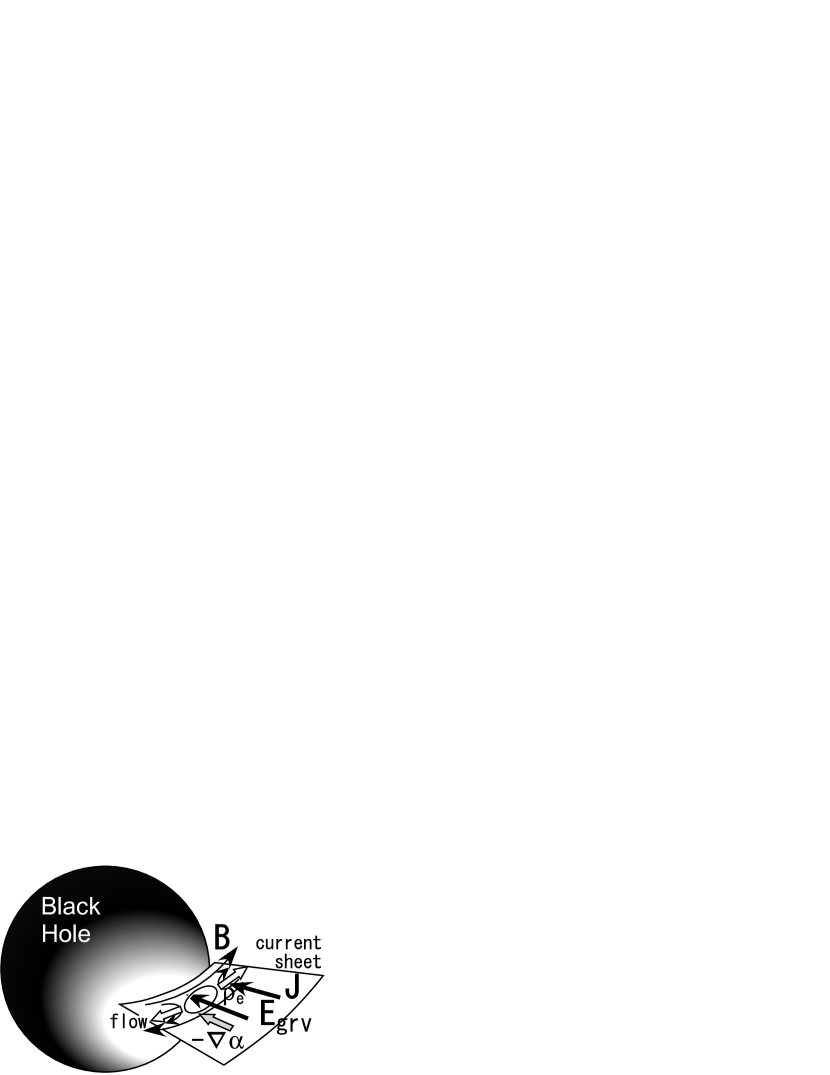
Figure 1: A schematic picture of the magnetic reconnection induced by the gravitational electromotive force. A pair of flow is induced by the magnetic reconnection.

The magnetic reconnection is expected to happen frequently in the black hole magnetospheres as suggested by a number of long-term ideal GRMHD simulations (Koide et al., 2000, 2006; McKinney, 2006). In spite of the artificial calculations of magnetic reconnection, it is not sure whether it makes whole numerical results with ideal GRMHD fatal, because the magnetic reconnection region, where the resistivity is significant, is very small compared to the global scale, and other regions are able to be treated by the ideal GRMHD. In such a case, causality would not be a so serious problem in the small region, and we would be able to use the ideal GRMHD for such situations. This speculation should be verified more carefully in near future.

The numerical simulation of the generalized GRMHD will be interesting. The equations of state (74) and (75) provide closures to the generalized GRMHD equations (60)-(68). Then, the numerical calculation is primarily possible, although it becomes drastically difficult compared to the ideal GRMHD simulations. This is because we have to treat the displacement current $\partial\mbox{\boldmath$E$}/\partial t$ in the Ampere’s law and the inertia of the current density $[1/(ne)]\partial[\{\mu h^{\ddagger}/(ne)\}\mbox{\boldmath$J$}]/\partial t$ in the generalized Ohm’s law explicitly. In the ideal GRMHD calculations, the former is taken into account implicitly and the latter can be neglected properly. Furthermore, we have to consider the zeroth component of the Ohm’s law to calculate the enthalpy density difference $\Delta h$ of relativistically hot plasmas around the black hole. Thus, appropriate simplification of the generalized GRMHD equations, especially of the simplified Ohm’s law, is required for numerical study. The modified resistive GRMHD may be one of the candidates.

In this last paragraph of this section, we investigate the possibility of the stationary Ohm’s law in a uniform plasma

$$\left(U^{\nu}-\frac{\Delta\mu}{ne}J^{\nu}\right){F^{\mu}}_{\nu}=\eta[J^{\mu}-\rho_{\rm e}^{\prime}(1+\Theta)U^{\mu}],$$ (124)

to consider the simplification of the generalized Ohm’s law (Equations (20) and (21)) for numerical simulations. The spatial components of the simplified Ohm’s law (124) are

$$\left(\gamma-\frac{\Delta\mu}{ne}\rho_{\rm e}\right)\mbox{\boldmath$E$}+\left(\mbox{\boldmath$U$}-\frac{\Delta\mu}{ne}\mbox{\boldmath$J$}\right)\times\mbox{\boldmath$B$}=\eta[\mbox{\boldmath$J$}-\rho_{\rm e}^{\prime}(1+\Theta)\mbox{\boldmath$U$}].$$ (125)

The temporal component of Equation (124) gives

$$\left(\mbox{\boldmath$U$}-\frac{\Delta\mu}{ne}\mbox{\boldmath$J$}\right)\cdot\mbox{\boldmath$E$}=\eta(\mbox{\boldmath$U$}\cdot\mbox{\boldmath$J$}^{\prime}-\rho_{\rm e}^{\prime}\gamma\Theta).$$ (126)

Here, we used the relation $J^{0}=\gamma\rho_{\rm e}^{\prime}+\mbox{\boldmath$U$}\cdot\mbox{\boldmath$J$}^{\prime}$. When we observe the quantities in the plasma center-of-mass frame, Equation (126) yields

$$\frac{\Delta\mu}{ne}(\mbox{\boldmath$J$}^{\prime}\cdot\mbox{\boldmath$E$}^{\prime})=\eta\rho_{\rm e}^{\prime}\Theta.$$ (127)

Using Equation (125) in the plasma rest frame, $\left(1-\frac{\Delta\mu}{ne}\rho_{\rm e}^{\prime}\right)\mbox{\boldmath$E$}^{\prime}-\frac{\Delta\mu}{ne}\mbox{\boldmath$J$}^{\prime}\times\mbox{\boldmath$B$}^{\prime}=\eta\mbox{\boldmath$J$}^{\prime},$ we obtain

$$\frac{\Delta\mu}{ne}\eta|\mbox{\boldmath$J$}^{\prime}|^{2}=\left(1-\frac{\Delta\mu}{ne}\rho_{\rm e}^{\prime}\right)\eta\rho_{\rm e}^{\prime}\Theta.$$ (128)

Assuming charge quasi-neutrality and non-relativistic collision between the two fluids, we substitute the approximation of $\Theta$ given by Equation (102) into Equation (128), then we find

$$\frac{\Delta\mu}{ne}\eta|\mbox{\boldmath$J$}^{\prime}|^{2}=\eta\rho_{\rm e}^{\prime}\frac{\theta\Delta\mu}{2e\rho_{\rm e}^{\prime}}\frac{|\mbox{\boldmath$J$}^{\prime}|^{2}}{n}=\frac{\theta\Delta\mu}{2ne}\eta|\mbox{\boldmath$J$}^{\prime}|^{2}.$$

This yields $\theta=2$ when $\Delta\mu\neq 0$ and Ohm heating is finite ($\eta|\mbox{\boldmath$J$}^{\prime}|^{2}>0$), while $\theta$ should be less than unity. This strange result even for the uniform plasma may suggest the stationary Ohm’s law contains a self-contradiction. This may come from the unbalance between thermal energy gain of the two fluids; otherwise, the non-dimensional variable $\Theta$ may have to be determined to keep its consistency. This should be clarified in near future.

Table 1: Necessary and sufficient conditions for approximation of the generalized GRMHD, the standard resistive GRMHD, and the ideal GRMHD approaches.

approach		conditions	effects neglected
generalized		$N_{\rm p}>N_{\rm crit}/\sqrt{2}$
GRMHD		($H<2$)
		(definition of the plasma, $N_{\rm p}\gg 1$)
standard			$\bullet$ current inertia in the Ohm’s law
resistive		$\omega_{\rm p}^{-1},\omega_{\rm c}^{-1}\ll L,\tau$	$\bullet$ current momentum transport
GRMHD			in the Ohm’s law
			$\bullet$ thermal electromotive force
			$\bullet$ centrifugal electromotive force
		$\sqrt{\mu}|\hat{\mbox{\boldmath$U$}}_{+}-\hat{\mbox{\boldmath$U$}}_{-}|\ll\hat{U}$	$\bullet$ charge inertia and current momentum
		$\sqrt{\mu}|n_{+}-n_{-}|\ll n$	in equations of motion and energy
		$\Delta\mu|\hat{\mbox{\boldmath$U$}}_{+}-\hat{\mbox{\boldmath$U$}}_{-}|\ll\hat{U}$	$\bullet$ the Hall effect
		$\theta\Delta\mu\left|\frac{\hat{\mbox{\boldmath$J$}}}{ne}\right|^{2}\ll\left|\frac{\rho_{\rm e}^{\prime}}{ne}\right|$	$\bullet$ frictionally thermalized energy equipartition
		$\omega_{\rm c}^{-1}\ll(g_{\rm BH})^{-1}$, $\mu\rho_{\rm e}<ne\hat{U}$	$\bullet$ gravitational electromotive force
		$\omega_{\rm p}^{-1},\omega_{\rm c}^{-1}\ll(\omega_{\rm BH}^{\dagger})^{-1}$	$\bullet$ frame-dragging electromotive force
		$\Delta p\ll\rho$, $\rho_{\rm e}^{\prime}\ll ne$ ($\Delta h\ll h$)	$\bullet$ zeroth component of the Ohm’s law
		$N_{\rm p}>N_{\rm crit}/\sqrt{2}$
		(condition of generalized GRMHD)
ideal		$S_{\rm M}\gg\frac{\gamma}{\sqrt{\mu}}$	$\bullet$ resistivity
GRMHD		and all the other conditions in the table

Table 2: Microscopic variables ($\omega_{\rm p}^{\rm e-i}$, $\omega_{\rm c}^{\rm e-i}$, $\cdots$), critical scales ($L_{\rm crit}$ and $\tau_{\rm crit}$), and characteristic scales of phenomena of plasmas around black holes ($g_{\rm BH}^{-1}$, $g_{\rm BH}^{-1}/c$, $L$, and $\tau$) to examine validity of the modified resistive GRMHD equations.

	GRB	BH X-ray binary	Supermassive BH in Galaxy	AGN
	GRB030329	LMC X-3	Sgr A*	M87
$M_{\rm BH}$ [$M_{\sun}$]	3	10	$2.6\times 10^{6}$	$3\times 10^{9}$
$\dot{M}$	0.1$M_{\sun}$ $\rm s^{-1}$	$10^{-8}M_{\sun}$ $\rm yr^{-1}$	$10^{-5}M_{\sun}$ $\rm yr^{-1}$	$10^{-2}M_{\sun}$ $\rm yr^{-1}$
$\rho$ [$\rm g\,cm^{-3}$]	$1.6\times 10^{10}$	0.0072	$1.5\times 10^{-6}$	$1.3\times 10^{-8}$
$T$ [K]	$1.2\times 10^{10}$	$1.8\times 10^{8}$	$3.5\times 10^{5}$	$7.1\times 10^{4}$
$B$ [G]	$2.7\times 10^{14}$	$1.1\times 10^{6}$	$1.4\times 10^{2}$	3.7
$\omega_{\rm p}^{\rm e-i}$ [$\rm s^{-1}$]	$5.4\times 10^{21}$	$3.6\times 10^{15}$	$5.3\times 10^{13}$	$4.9\times 10^{12}$
$\omega_{\rm c}^{\rm e-i}$ [$\rm s^{-1}$]	$2.5\times 10^{18}$	$1.0\times 10^{10}$	$1.3\times 10^{6}$	$3.5\times 10^{4}$
$1/\omega_{\rm p}^{\rm e-i}$ [s]	$1.9\times 10^{-22}$	$2.8\times 10^{-16}$	$1.9\times 10^{-14}$	$2.0\times 10^{-13}$
$1/\omega_{\rm c}^{\rm e-i}$ [s]	$4.0\times 10^{-19}$	$1.0\times 10^{-10}$	$7.7\times 10^{-9}$	$2.9\times 10^{-5}$
$c/\omega_{\rm p}^{\rm e-i}$ [m]	$5.6\times 10^{-14}$	$8.3\times 10^{-8}$	$5.7\times 10^{-6}$	$6.1\times 10^{-5}$
$c/\omega_{\rm c}^{\rm e-i}$ [m]	$1.2\times 10^{-10}$	0.030	230	$8.6\times 10^{3}$
$L_{\rm crit}$ [m]	$5.6\times 10^{-10}$	0.030	230	8600
$\tau_{\rm crit}$ [s]	$4.0\times 10^{-19}$	$1.0\times 10^{-10}$	$7.7\times 10^{-9}$	$2.9\times 10^{-5}$
$g_{\rm BH}^{-1}\sim r_{\rm S}$ [m]	$9.0\times 10^{3}$	$3.0\times 10^{4}$	$7.8\times 10^{9}$	$9.0\times 10^{11}$
$g_{\rm BH}^{-1}/c\sim r_{\rm S}/c$ [s]	$3.0\times 10^{-5}$	$1.0\times 10^{-4}$	26	3000
$L\gtrsim L_{\rm CS}$ [m]	480	10	$2.3\times 10^{4}$	$7.5\times 10^{5}$
$\tau\gtrsim L_{\rm CS}/c$ [s]	$1.6\times 10^{-6}$	$3.3\times 10^{-8}$	$7.7\times 10^{-5}$	$2.5\times 10^{-3}$

Appendix A 3+1 formalism of divergence of tensors

We derive a 3+1 formalism of the covariant equation

$$\nabla_{\nu}S^{\mu\nu}=H^{\mu},$$ (A1)

for the arbitrary symmetric tensor $S^{\mu\nu}$, which satisfies $S^{\mu\nu}=S^{\nu\mu}$. We have the relations between any tensor $S^{\mu\nu}$ and the corresponding tensor observed by the ZAMO frame $\hat{S}^{\mu\nu}$,

$$S^{00}=\frac{1}{\alpha^{2}}\hat{S}^{00},\verb! !S^{i0}=S^{0i}=\frac{1}{\alpha h_{i}}(\hat{S}^{0i}+\beta^{i}\hat{S}^{00}),\verb! !S^{ij}=\frac{1}{h_{i}h_{j}}(\hat{S}^{ij}+\beta^{i}\hat{S}^{0j}+\beta^{j}\hat{S}^{i0}+\beta^{i}\beta^{j}\hat{S}^{00}).$$ (A2)

Using $\Gamma_{\mu\lambda}^{\lambda}=\partial_{\mu}(\log\sqrt{-g})$, we obtain

$$\nabla_{\nu}S^{\mu\nu}=\frac{1}{\sqrt{-g}}\frac{\partial}{\partial x^{\nu}}\left(\sqrt{-g}S^{\mu\nu}\right)+\Gamma_{\sigma\nu}^{\mu}S^{\sigma\nu}.$$ (A3)

With the symmetry of $S^{\mu\nu}$, we have

$$\Gamma_{\nu\lambda}^{\mu}S^{\lambda\nu}=-\frac{1}{2}g^{\mu j}(\partial_{j}g_{\kappa\lambda})S^{\lambda\kappa}+g^{\mu\lambda}(\partial_{j}g_{\kappa\lambda})S^{\kappa j}.$$ (A4)

Using Equations (A2) and (A4), we get

$$\Gamma_{\sigma\nu}^{\mu}S^{\sigma\nu} = \left[\frac{A^{\mu}}{\alpha^{2}}+\sum_{j}\frac{\beta^{j}}{\alpha h_{j}}B_{j}^{\mu}+\sum_{j,k}\frac{\beta^{j}\beta^{k}}{h_{j}h_{k}}C_{kj}^{\mu}+\sum_{j}\left(\frac{\beta^{j}}{h_{j}}\right)^{2}D_{j}^{\mu}\right]\hat{S}^{00}$$

$$+ \sum_{j}\frac{1}{h_{j}}\left[\frac{B^{\mu}}{\alpha}+\sum_{k}\frac{\beta^{k}}{h_{k}}C_{jk}^{\mu}+\sum_{k}\frac{\beta^{k}}{h_{k}}C_{jk}^{\mu}+2\frac{\beta^{j}}{h_{j}}D_{j}^{\mu}\right]\hat{S}^{j0}$$

$$+ \sum_{j,k}\frac{1}{h_{j}h_{k}}C_{kj}^{\mu}\hat{S}^{kj}+\sum_{j}\frac{1}{h_{j}^{2}}D_{j}^{\mu}\hat{S}^{jj},$$

where

$$A^{\mu} = -\sum_{l}\frac{1}{2}g^{\mu l}(\partial_{l}g_{00}),$$

$$B_{j}^{\mu} = g^{\mu 0}(\partial_{j}g_{00})+\sum_{l}g^{\mu l}(\partial_{j}g_{0l}-\partial_{l}g_{0j}),$$

$$C_{kj}^{\mu} = g^{\mu 0}(\partial_{j}g_{k0})+g^{\mu k}(\partial_{j}g_{kk}),$$ (A6)

$$D_{j}^{\mu} = -\sum_{l}\frac{1}{2}g^{\mu l}(\partial_{l}g_{jj}).$$

Using Equations (31), (33), and (35) of $h_{i}$, $\beta^{i}$, and $\alpha$, we have

$$A^{i} = \frac{1}{2h_{i}}\partial_{i}h_{0}^{2}-\sum_{l}\frac{1}{2h_{i}h_{l}}\beta^{i}\beta^{l}\partial_{l}h_{0}^{2},$$

$$B_{j}^{i} = \frac{\beta^{i}}{\alpha h_{i}}\partial_{j}h_{0}^{2}+\frac{1}{h_{i}^{2}}\left[-\partial_{j}(h_{i}\alpha\beta^{i})+\partial_{i}(h_{j}\alpha\beta^{j})\right]-\sum_{l}\frac{\beta^{i}\beta^{l}}{h_{i}h_{l}}\left[-\partial_{j}(h_{l}\alpha\beta^{l})+\partial_{l}(h_{j}\alpha\beta^{j})\right],$$

$$C_{kj}^{i} = \frac{\beta^{i}}{\alpha h_{i}}\partial_{j}(h_{k}\alpha\beta^{k})+\frac{\delta^{ik}}{h_{i}^{2}}\partial_{j}h_{i}^{2}-\frac{\beta^{i}\beta^{k}}{h_{i}h_{k}}\partial_{j}h_{k}^{2},$$ (A7)

$$D_{j}^{i} = -\frac{1}{2h_{i}^{2}}\partial_{i}h_{j}^{2}+\sum_{l}\frac{\beta^{i}\beta^{l}}{2h_{i}h_{l}}\partial_{l}h_{j}^{2},$$

$$A^{0} = -\sum_{j}\frac{\beta_{j}}{2\alpha h_{j}}\partial_{j}h_{0}^{2},$$

$$B_{j}^{0} = \frac{1}{\alpha^{2}}\partial_{j}h_{0}^{2}-\sum_{k}\frac{\beta^{k}}{\alpha h_{k}}\left[-\partial_{j}(h_{k}\alpha\beta^{k})+\partial_{k}(h_{j}\alpha\beta^{j})\right],$$

$$C_{kj}^{0} = \frac{1}{\alpha^{2}}\partial_{j}(h_{k}\alpha\beta^{k})-\frac{\beta^{k}}{\alpha h_{k}}\partial_{j}h_{k}^{2},$$

$$D_{j}^{0} = \sum_{k}\frac{\beta^{k}}{2\alpha h_{k}^{2}}\partial_{k}h_{j}^{2}.$$

Then, we get

$$\frac{\partial}{\partial t}(\hat{S}^{i0}+\beta^{i}\hat{S}^{00})+\frac{1}{h_{1}h_{2}h_{3}}\sum_{j}\frac{\partial}{\partial x^{\nu}}\left[\frac{\sqrt{-g}}{h_{j}}\left(\hat{S}^{ij}+\beta^{i}\hat{S}^{0j}+\beta^{j}\hat{S}^{i0}+\beta^{i}\beta^{j}\hat{S}^{00}\right)\right]$$ (A8)

$$-\sum_{j}\frac{\alpha}{h_{i}h_{j}}\frac{\partial h_{i}}{\partial x^{j}}\left(\hat{S}^{ij}+\beta^{i}\hat{S}^{0j}+\beta^{j}\hat{S}^{i0}+\beta^{i}\beta^{j}\hat{S}^{00}\right)+\alpha h_{i}\Gamma_{\nu\lambda}^{i}S^{\lambda\nu}=\alpha(\hat{H}^{i}+\beta^{i}\hat{H}^{0}),$$

$$\frac{\partial}{\partial t}\hat{S}^{00}+\frac{1}{h_{1}h_{2}h_{3}}\sum_{j}\frac{\partial}{\partial x^{j}}\left[\frac{\sqrt{-g}}{h_{j}}\left(\hat{S}^{0j}+\beta^{j}\hat{S}^{00}\right)\right]$$ (A9)

$$-\sum_{j}\frac{1}{h_{j}}\frac{\partial\alpha}{\partial x^{j}}\left(\hat{S}^{0j}+\beta^{j}\hat{S}^{00}\right)+\alpha^{2}\Gamma_{\nu\lambda}^{0}S^{\lambda\nu}=\alpha\hat{H}^{0}.$$

Subtracting Equation (A9) multiplied by $\beta^{i}$ from Equation (A9), we have

$$\frac{\partial}{\partial t}\hat{S}^{i0}+\frac{1}{h_{1}h_{2}h_{3}}\sum_{j}\frac{\partial}{\partial x^{j}}\left[\frac{\sqrt{-g}}{h_{j}}\left(\hat{S}^{ij}+\beta^{j}\hat{S}^{i0}\right)\right]$$

$$-\sum_{j}\frac{\alpha}{h_{i}h_{j}}\frac{\partial h_{i}}{\partial x^{j}}\left(\hat{S}^{ij}+\beta^{i}\hat{S}^{0j}+\beta^{j}\hat{S}^{i0}+\beta^{i}\beta^{j}\hat{S}^{00}\right)+\sum_{j}\frac{1}{h_{j}}\frac{\partial}{\partial h_{j}}(\alpha\beta^{i})\left(\hat{S}^{0j}+\beta^{j}\hat{S}^{00}\right)$$

$$+\alpha h_{i}\Gamma_{\nu\lambda}^{i}S^{\lambda\nu}-\beta^{i}\alpha^{2}\Gamma_{\nu\lambda}^{0}S^{\lambda\nu}=\alpha\hat{H}^{i}.$$ (A10)

Substituting Equations (A) and (A7) into Equations (A9) and (A10), we finally obtain

$$\frac{\partial}{\partial t}\hat{S}^{00}+\frac{1}{h_{1}h_{2}h_{3}}\sum_{j}\frac{\partial}{\partial x^{j}}\left[\frac{\alpha h_{1}h_{2}h_{3}}{h_{j}}\left(\hat{S}^{0j}+\beta^{j}\hat{S}^{00}\right)\right]+\sum_{j}\frac{1}{h_{j}}\frac{\partial\alpha}{\partial x^{j}}\hat{S}^{j0}$$

$$+\sum_{j,k}\alpha\beta^{k}(G_{kj}\hat{S}^{kj}-G_{jk}\hat{S}^{jj})+\sum_{j,k}\sigma_{jk}\hat{S}^{jk}=\alpha\hat{H}^{0},$$ (A11)

$$\frac{\partial}{\partial t}\hat{S}^{i0}+\frac{1}{h_{1}h_{2}h_{3}}\sum_{j}\frac{\partial}{\partial x^{j}}\left[\frac{\alpha h_{1}h_{2}h_{3}}{h_{j}}\left(\hat{S}^{ij}+\beta^{j}\hat{S}^{i0}\right)\right]+\frac{1}{h_{i}}\frac{\partial\alpha}{\partial x^{i}}\hat{S}^{00}$$

$$-\sum_{j}\alpha\left[G_{ij}\hat{S}^{ij}-G_{ji}\hat{S}^{jj}+\beta^{j}(G_{ij}\hat{S}^{0i}-G_{ji}\hat{S}^{0j})\right]+\sum_{j}\sigma_{ji}\hat{S}^{0j}=\alpha\hat{H}^{i}.$$ (A12)

Appendix B Dispersion relation of electromagnetic wave in unmagnetized plasma

We derive the dispersion relation of the electromagnetic wave in a uniform, unmagnetized plasma with $\rho=\bar{\rho}$, $U^{\mu}=(1,0,0,0)$, $p=\bar{p}$, $h=\bar{h}$, $\Delta h=\Delta\bar{h}$, $\Delta p=\Delta\bar{p}$, $F_{\mu\nu}=0$, and $J^{\mu}=0$ in the Minkowski space-time. When perturbations due to the electromagnetic wave to the uniform variables are written by $\tilde{\rho}=\rho-\bar{\rho}$, $\tilde{p}=p-\bar{p}$, $\tilde{h}=h-\bar{h}$, $\Delta\tilde{h}=\Delta h-\Delta\bar{h}$, $\Delta\tilde{p}=\Delta p-\Delta\bar{p}$, $\tilde{U}^{\mu}=(0,\tilde{\mbox{\boldmath$U$}})$, $\tilde{F}_{\mu\nu}=F_{\mu\nu}$ ($\tilde{\mbox{\boldmath$E$}}=\mbox{\boldmath$E$}$, $\tilde{\mbox{\boldmath$B$}}=\mbox{\boldmath$B$}$), $\tilde{J}^{\mu}=J^{\mu}$, we have the linearized equations in the 3-vector form,

$$\frac{\partial}{\partial t}\tilde{\rho}+\bar{\rho}\nabla\cdot\tilde{\mbox{\boldmath$U$}} = 0,$$ (B1)

$$\frac{\partial}{\partial t}\tilde{h}+\frac{4\mu\Delta h}{\bar{n}e}\frac{\partial}{\partial t}\tilde{\rho}_{\rm e}-\frac{\partial}{\partial t}\tilde{p}+\bar{h}\nabla\cdot\tilde{\mbox{\boldmath$U$}}+\frac{2\mu\Delta\bar{h}}{\bar{n}e}\nabla\cdot\tilde{\mbox{\boldmath$J$}} = 0,$$ (B2)

$$\bar{h}\frac{\partial}{\partial t}\tilde{\mbox{\boldmath$U$}}+\frac{2\mu\Delta\bar{h}}{\bar{n}e}\frac{\partial}{\partial t}\tilde{\mbox{\boldmath$J$}} = -\nabla\tilde{p},$$ (B3)

$$\frac{\mu\bar{h}^{\ddagger}}{(\bar{n}e)^{2}}\frac{\partial}{\partial t}\tilde{\mbox{\boldmath$J$}}+\frac{2\mu\Delta\bar{h}}{\bar{n}e}\frac{\partial}{\partial t}\tilde{\mbox{\boldmath$U$}} = \frac{1}{2\bar{n}e}\nabla(\Delta\mu\tilde{p}-\Delta\tilde{p})+\tilde{\mbox{\boldmath$E$}}-\eta\tilde{\mbox{\boldmath$J$}},$$ (B4)

$$\frac{\bar{h}^{\ddagger}}{2(\bar{n}e)^{2}}\frac{\partial}{\partial t}\tilde{\rho}_{\rm e}+\frac{1}{2\bar{n}e}\frac{\partial}{\partial t}\Delta\tilde{h}+\frac{1}{8\mu\bar{n}e}\frac{\partial}{\partial t}(\Delta\mu\tilde{p}-\Delta\tilde{p}) + \frac{\bar{h}^{\ddagger}}{(2\bar{n}e)^{2}}\nabla\cdot\tilde{\mbox{\boldmath$J$}}+\frac{\Delta\bar{h}}{2\bar{n}e}\nabla\cdot\tilde{\mbox{\boldmath$U$}}=0,$$ (B5)

$$\nabla\cdot\tilde{\mbox{\boldmath$E$}} = \tilde{\rho}_{\rm e},$$ (B6)

$$\nabla\cdot\tilde{\mbox{\boldmath$B$}} = 0,$$ (B7)

$$\frac{\partial}{\partial t}\tilde{\mbox{\boldmath$B$}} = -\nabla\times\tilde{\mbox{\boldmath$E$}},$$ (B8)

$$\tilde{\mbox{\boldmath$J$}}+\frac{\partial}{\partial t}\tilde{\mbox{\boldmath$E$}} = \nabla\times\tilde{\mbox{\boldmath$B$}}.$$ (B9)

In this Appendix, we note an equilibrium variable with a bar, and a perturbation with a tilde. We also assume the resistivity is uniform and constant, and the perturbation of any variable $\tilde{A}$ is proportional to $\exp(i\mbox{\boldmath$k$}\cdot\mbox{\boldmath$r$}-i\omega t)=\exp(i\eta_{\mu\nu}k^{\mu}x^{\nu})$, where $k^{\mu}=(\omega,\mbox{\boldmath$k$})$ is the constant contravariant vector called the wave number 4-vector. For simplicity, we investigate the transverse mode of the electromagnetic wave in an unmagnetized plasma, thus we set

$$\tilde{\mbox{\boldmath$E$}},\verb! !\tilde{\mbox{\boldmath$B$}},\verb! !\tilde{\mbox{\boldmath$U$}}\verb! !\perp\verb! !\mbox{\boldmath$k$}.$$ (B10)

Then, we have the following linearized equations:

$$\tilde{\rho} = 0,$$ (B11)

$$\hskip 28.45274pt\tilde{h}+\frac{4\mu\Delta\tilde{h}}{\bar{n}e} - \tilde{p}=0,$$ (B12)

$$4\mu\left(\frac{\bar{h}^{\ddagger}}{\bar{n}e}\tilde{\rho}_{\rm e}+\Delta\tilde{h}\right) + \Delta\mu\tilde{p}-\Delta\tilde{p}=0,$$ (B13)

$$-i\omega\left(\bar{h}\tilde{\mbox{\boldmath$U$}}+\frac{2\mu\Delta\bar{h}}{\bar{n}e}\tilde{\mbox{\boldmath$J$}}\right) = \mbox{\boldmath$0$},$$ (B14)

$$-i\omega\frac{\mu}{\bar{n}e}\left(\frac{\bar{h}^{\ddagger}}{\bar{n}e}\tilde{\mbox{\boldmath$J$}}+2\Delta\bar{h}\tilde{\mbox{\boldmath$U$}}\right) = \tilde{\mbox{\boldmath$E$}}-\eta\tilde{\mbox{\boldmath$J$}},$$ (B15)

$$-i\omega\tilde{\mbox{\boldmath$B$}} = -i\mbox{\boldmath$k$}\times\tilde{\mbox{\boldmath$E$}},$$ (B16)

$$\tilde{\mbox{\boldmath$J$}}-i\omega\tilde{\mbox{\boldmath$E$}} = i\mbox{\boldmath$k$}\times\tilde{\mbox{\boldmath$B$}},$$ (B17)

$$\tilde{\rho}_{\rm e}=0.$$ (B18)

After some algebraic calculations, we obtain the dispersion relation of the electromagnetic wave,

$$\left[\eta-i\omega\frac{\mu}{(\bar{n}e)^{2}\bar{h}}\left(\bar{h}^{\ddagger}\bar{h}-4\mu(\Delta\bar{h})^{2}\right)\right](k^{2}-\omega^{2})=i\omega.$$ (B19)

This dispersion equation is identical to that of the electromagnetic wave in the pair plasma when we regard $4\mu(\bar{h}^{\ddagger}-4\mu(\Delta\bar{h})^{2}/\bar{h})$ as the enthalpy density $h$ in Koide (2008). Koide (2008) proved that the group velocity of the dispersion relation (Equation (B19)) is less than or equal to the light speed if

$$H=\frac{(\bar{n}e\eta)^{2}}{\mu[\bar{h}^{\ddagger}-4\mu(\Delta\bar{h})^{2}/\bar{h}]}<2.$$ (B20)

Appendix C Relation between $H$ and plasma parameter

We show the relation between $H$ and the plasma parameter. Using the definition of $h^{\ddagger}$ and $\Delta h$ (Equations (13) and (16)), we have

$$\frac{\mu[hh^{\ddagger}-4\mu(\Delta h)^{2}]}{h}=n^{4}\frac{h_{+}h_{-}}{(n_{+}n_{-})^{2}h}.$$ (C1)

From Equation (B20), we obtain

$$H=\left(\frac{\eta e}{n}\right)^{2}\frac{(n_{+}n_{-})^{2}h}{h_{+}h_{-}},$$ (C2)

where we omit the bars on the mean variables. We consider the nonrelativistic situations where the classical resistivity,

$$\eta=\frac{e^{2}}{2\pi\mu m}\frac{\ln\Lambda}{v_{r}^{3}},$$ (C3)

is valid (Bellan, 2006), where $v_{r}$ is the average relative velocity of the two fluid particles and $\ln\Lambda$ is the Coulomb logarithm, which is an order of 10. We use the expression of the averaged velocity by

$$v_{r}=\left(f_{+}\frac{p_{+}}{m_{+}n_{+}}+f_{-}\frac{p_{-}}{m_{-}n_{-}}\right)^{1/2},$$ (C4)

where $f_{\pm}$ is the degrees of the freedom of the two fluid particles. Then, we give the expression of the resistivity by

$$\eta=\frac{e^{2}\ln\Lambda}{2\pi\mu m}\left(f_{+}\frac{p_{+}}{m_{+}n_{+}}+f_{-}\frac{p_{-}}{m_{-}n_{-}}\right)^{-3/2}.$$ (C5)

Here, we define the plasma parameter of the plasma with/without the charge neutrality by

$$N_{\rm p}=\sqrt{n_{+}n_{-}}\lambda_{\rm D}^{3},$$ (C6)

where $\lambda_{\rm D}$ is the Debye length (see Bellan, 2006),

$$\frac{1}{\lambda_{\rm D}^{2}}=\frac{(n_{+}e)^{2}}{p_{+}}+\frac{(n_{-}e)^{2}}{p_{-}}.$$ (C7)

In general, we define the plasma as a particle ensemble where the Debye cube contains a plenty of both positively and negatively charged particles,

$$n_{+}\lambda_{\rm D}^{3}\gg 1,\verb! !n_{-}\lambda_{\rm D}^{3}\gg 1.$$ (C8)

Therefore, we use the condition of the plasma $N_{\rm p}\gg 1$ as far as we consider the plasma. Using the inequality of the arithmetic mean and geometric mean

$$\frac{1}{2}\left[f_{+}\frac{p_{+}}{m_{+}n_{+}}+f_{-}\frac{p_{-}}{m_{+}n_{-}}\right] \geq \sqrt{f_{+}\frac{p_{+}}{m_{+}n_{+}}f_{-}\frac{p_{-}}{m_{+}n_{-}}},$$

$$\frac{1}{2}\left[\frac{n_{+}^{2}}{p_{+}}+\frac{n_{-}^{2}}{p_{-}}\right] \geq \sqrt{\frac{n_{+}^{2}}{p_{+}}\frac{n_{-}^{2}}{p_{-}}},$$

we get

$$HN_{\rm p}^{2}\leq\frac{m_{+}n_{-}+m_{-}n_{+}}{m\sqrt{n+n_{-}}}\left[2^{6}\left(\frac{2\pi}{\ln\Lambda}\right)^{2}(f_{+}f_{-})^{3/2}\mu^{3/2}\right]^{-1}<\left[2^{8}\left(\frac{\pi}{\ln\Lambda}\right)^{2}\mu^{3/2}\zeta^{1/2}\right]^{-1}\equiv N_{\rm crit}^{2},$$ (C9)

because $f_{\pm}\geq 1$, where $\zeta$ is the variable related to the charge neutrality, $\zeta\equiv n_{+}n_{-}/(n_{+}+n_{-})^{2}$. For the neutral plasma, $\zeta$ is 1/4 and $\zeta$ decreases as the break of the charge neutrality gets stronger. Then, if $N_{\rm p}>N_{\rm crit}/\sqrt{2}$, we confirm $H<2$. Here, we evaluate $N_{\rm crit}$ as

$$N_{\rm crit}=\frac{\ln\Lambda}{2^{4}\pi}\mu^{-3/4}\zeta^{-1/4}.$$ (C10)

Eventually, we have the scaling

$$N_{\rm crit} = 0.281\mu^{-3/4}\left(\frac{\ln\Lambda}{10}\right)\left(\frac{\zeta}{1/4}\right)^{-1/4}$$ (C11)

$$= \left\{\begin{array}[]{cl}84\left(\frac{\ln\Lambda}{10}\right)\left(\frac{\zeta}{1/4}\right)^{-1/4}&(\mbox{for electron-ion plasma},\;\mu=5\times 10^{-4})\\ 0.80\left(\frac{\ln\Lambda}{10}\right)\left(\frac{\zeta}{1/4}\right)^{-1/4}&(\mbox{for pair plasma},\;\mu=1/4)\end{array}\right..$$ (C14)

When $N_{\rm p}$ is so large that $N_{\rm p}>N_{\rm crit}/\sqrt{2}$, causality of the GRMHD equations (Equations (18)-(20), (3), and (4)) is satisfied.

References

• Bekenstein & Oron (1978) Bekenstein, J. & Oron, E. 1978, Phys.Β Rev.Β D, 18, 1809.
• Bellan (2006) Bellan, P. M. 2006, Fundamentals of Plasma Physics, (Cambridge: Cambridge Univ. Press).
• Chandrasekhar (1938) Chandrasekhar, S. 1938, An Introduction to the Study of Stellar Structure (New York: Dover).
• Gammie et al. (2003) Gammie, C. F., McKinney, J. C., & Toth, G. 2003, ApJ, 589, 444.
• Khanna (1998) Khanna, R. l998, MNRAS, 294, 673.
• Khanna & Camenzind (1994) Khanna, R. & Camenzind, M. l994, ApJ, 435, L129.
• Khanna & Camenzind (1996a) Khanna, R. & Camenzind, M. l996a, A&A, 307, 665.
• Khanna & Camenzind (1996b) Khanna, R. & Camenzind, M. l996b, A&A, 313, 1028.
• Koide (2003) Koide, S. 2003, Phys.Β Rev.Β D, 67, 104010.
• Koide (2004) Koide, S., 2004, ApJ, 606, L45.
• Koide (2008) Koide, S. 2008, Phys.Β Rev.Β D, 78, 125026.
• Koide (2009) Koide, S. 2009, ApJ, 696, 2220.
• Koide & Arai (2008) Koide, S. & Arai, K. 2008, ApJ, 682, 1124.
• Koide et al. (2000) Koide, S., Meier, D. L., Shibata, K., & Kudoh, T. 2000, ApJ, 536, 668.
• Koide et al. (1996) Koide, S. Nishikawa, K.-I. and Mutel, R. L. 1996, ApJ, 463, L71.
• Koide et al. (1998) Koide, S., Shibata, K., & Kudoh, T. 1998, ApJ, 495, L63.
• Koide et al. (1999) Koide, S., Shibata, K., & Kudoh, T. 1999, ApJ, 522, 727.
• Koide et al. (2006) Koide, S., Shibata, K., & Kudoh, T. 2006, Phys.Β Rev.Β D, 74, 044005.
• Koide et al. (2002) Koide, S., Shibata, K., Kudoh, T., & Meier, D. L. 2002, Science, 295, 1688.
• Kudoh & Kaburaki (1996) Kudoh, T., & Kaburaki, O. 1996, ApJ, 460, 199.
• McKinney (2004) McKinney, J. C., 2004, PhD thesis, Univ. Illinois.
• McKinney (2006) McKinney, J. C. 2006, MNRAS, 368, 1561.
• Meier (2004) Meier, D. L. 2004, ApJ, 605, 340.
• Shibata et al. (1999) Shibata, K., Fukue, J., Matsumoto, R., & Mineshige, S. 1999, Active Universe (Tokyo: Shokabo) (in Japanese).
• Synge (1957) Synge, J. L. 1957, The Relativistic Gas (Amsterdam: North Holland).
• Thorne et al. (1986) Thorne, K. S., Price, R. H., and Macdonald, D. A. 1986 Membrane Paradigm (New Haven: Yale Univ. Press).
• Watanabe et al. (2006) Watanabe, N., & Yokoyama, T. 2006, ApJ, 647, L123.