Tetraquark interpretation of the Belle data on the anomalous $\Upsilon(1S)\pi^{+}\pi^{-}$ and $\Upsilon(2S)\pi^{+}\pi^{-}$ production near the $\Upsilon(5S)$ resonance

Abstract

We analyze the Belle data [K. F. Chen et al. (Belle Collaboration), Phys. Rev. Lett.  100, 112001 (2008); I. Adachi et al. (Belle Collaboration), arXiv:0808.2445] on the processes $e^{+}e^{-}\to\Upsilon(1S)\;\pi^{+}\pi^{-},\Upsilon(2S)\;\pi^{+}\pi^{-}$ near the peak of the $\Upsilon(5S)$ resonance, which are found to be anomalously large in rates compared to similar dipion transitions between the lower $\Upsilon$ resonances. Assuming these final states arise from the production and decays of the $J^{PC}=1^{--}$ state $Y_{b}(10890)$, which we interpret as a bound (diquark-antidiquark) tetraquark state $[bq][\bar{b}\bar{q}]$, a dynamical model for the decays $Y_{b}\to\Upsilon(1S)\;\pi^{+}\pi^{-},\Upsilon(2S)\;\pi^{+}\pi^{-}$ is presented. Depending on the phase space, these decays receive significant contributions from the scalar $0^{++}$ states, $f_{0}(600)$ and $f_{0}(980)$, and from the $2^{++}$ $q\bar{q}$-meson $f_{2}(1270)$. Our model provides excellent fits for the decay distributions, supporting $Y_{b}$ as a tetraquark state.

The observation of the $\Upsilon(1S)\;\pi^{+}\pi^{-}$ and $\Upsilon(2S)\;\pi^{+}\pi^{-}$ states near the $\Upsilon(5S)$ resonance peak at $\sqrt{s}=10.87$ GeV at the KEKB $e^{+}e^{-}$ collider by the Belle collaboration Abe:2007tk has received a lot of theoretical attention Hou:2006it . The two puzzling features of these data are that, if interpreted in terms of the processes $e^{+}e^{-}\to\Upsilon(5S)\to\Upsilon(1S)\;\pi^{+}\pi^{-},\Upsilon(2S)\;\pi^{+}\pi^{-}$, the rates are anomalously larger (by more than two orders of magnitude) than the expectations from scaling the comparable $\Upsilon(4S)$ decays to the $\Upsilon(5S)$, and the shapes of the distributions in the dipion invariant mass $m_{\pi\pi}$ and the cosine of the helicity angle, $\cos\theta$, where $\theta$ is the angle between the $\pi^{-}$ and $\Upsilon(5S)$ in the dipion rest frame, are not described by the models Brown:1975dz based on the QCD multipole expansion Gottfried:1977gp ; Kuang:2006me - a feature also at variance with similar dipion transitions between lower $\Upsilon$ resonances. A critical observation towards understanding these features is that the final states in question are produced not from the decays of $\Upsilon(5S)$, but from the process $e^{+}e^{-}\to Y_{b}(10890)\to\Upsilon(1S)\;\pi^{+}\pi^{-},\Upsilon(2S)\;\pi^{+}\pi^{-}$, with $Y_{b}$ a $1^{--}$ state, having a total decay width $\Gamma(Y_{b})=55\pm 9$ MeV Olsen:2009gi . In a closely related recent paper Ali:2009pi , we have analyzed the BaBar data :2008hx obtained at the SLAC B factory during an energy scan of the $e^{+}e^{-}\to b\bar{b}$ cross section in the range of the center of mass energy $\sqrt{s}=10.54$ to 11.20 GeV, observing that the BaBar data on the $R_{b}$-scan are consistent with the presence of an additional $b\bar{b}$ state $Y_{[bq]}$ with a mass of 10.90 GeV and a width of about 30 MeV, apart from the $\Upsilon(5S)$ and $\Upsilon(6S)$ resonances. Identifying the $J^{PC}=1^{--}$ state $Y_{[bq]}(10900)$ seen in the energy scan of the $e^{+}e^{-}\to b\bar{b}$ cross section by BaBar :2008hx with the state $Y_{b}(10890)$ seen by Belle Abe:2007tk , we present a dynamical model based on the tetraquark interpretation of $Y_{b}(10890)$ and show that it is in excellent agreement with the measured distributions in the decays $Y_{b}\to\Upsilon(1S)\;\pi^{+}\pi^{-},\Upsilon(2S)\;\pi^{+}\pi^{-}$.

In the tetraquark interpretation, $Y_{[bq]}$ is a $J^{PC}=1^{--}$ bound (diquark-antidiquark) state having the flavor content $Y_{[bq]}={\cal Q}{\bar{\cal Q}}=[bq][\bar{b}\bar{q}]$ (here $q=u$ or $q=d$, and $\cal Q$ is a diquark) with the spin and orbital momentum quantum numbers: $S_{\cal Q}=0,~{}S_{\bar{\cal Q}}=0,~{}S_{\cal Q\bar{\cal Q}}=0,~{}L_{\cal Q\bar{\cal Q}}=1$ Drenska:2008gr . The first two quantum numbers are the diquark spin, antidiquark spin, respectively, and the last two denote the spin and the orbital angular quantum numbers of the tetraquarks, with the total spin being $J=S_{\cal Q\bar{\cal Q}}+~{}L_{\cal Q\bar{\cal Q}}=1$. Such spin-0 diquarks are called “good” diquarks Jaffe:1976ih and an interpolating diquark operator can be written as ${\cal Q}_{i\alpha}=\epsilon_{\alpha\beta\gamma}(\bar{b}_{c}^{\beta}\gamma_{5}q_{i}^{\gamma}-\bar{q}_{i_{c}}^{\beta}\gamma_{5}b^{\gamma})$ (with $q_{i}=u,d$ for $i=1,2$ and $\bar{b}_{c}$ the charge conjugate $b$-quark field $\bar{b}_{c}=-ib^{\rm T}\sigma_{2}\gamma_{5}$). The “good” diquark ${\cal Q}_{i\alpha}$ is in the attractive anti-triplet ($\bar{3}$) color channel (with the color quantum numbers denoted by the Greek letters). There are two such $J^{PC}=1^{--}$ states, $Y_{[bq]}=([bq]_{S=0}[\bar{b}\bar{q}]_{S=0})_{\rm P-wave}$, with the mass eigenstates, called $Y_{[b,l]}$ and $Y_{[b,h]}$ in  Ali:2009pi , being orthogonal combinations of $Y_{[bu]}$ and $Y_{[bd]}$. Their mass difference is induced by isospin splitting $m_{d}-m_{u}$ and a mixing angle and is estimated as $\Delta M(Y_{b})=(5.6\pm 2.8)$ MeV. In the following, we will not distinguish between the lighter and the heavier of these states and denote them by the common symbol $Y_{b}$. The decays $Y_{b}\to\Upsilon(1S)\;\pi^{+}\pi^{-},\Upsilon(2S)\;\pi^{+}\pi^{-}$ are sub-dominant, but Zweig-allowed and involve essentially the quark rearrangements shown below.

With the $J^{PC}$ of the $Y_{b}$ and $\Upsilon(nS)$ both $1^{--}$, the $\pi^{+}\pi^{-}$ states in the decays $Y_{b}\to\Upsilon(1S)\;\pi^{+}\pi^{-},\Upsilon(2S)\;\pi^{+}\pi^{-}$ are allowed to have the $0^{++}$ and $2^{++}$ quantum numbers. There are only three low-lying states in the Particle Data Group (PDG) Amsler:2008zzb which can contribute as intermediate states, namely the two $0^{++}$ states, $f_{0}(600)$ and $f_{0}(980)$, which, following Hooft:2008we ; Maiani:2004uc , we take as the lowest tetraquark states, and the $2^{++}$ $q\bar{q}$-meson state $f_{2}(1270)$, all of which decay dominantly into $\pi\pi$. For the decay $Y_{b}\to\Upsilon(1S)\;\pi^{+}\pi^{-}$, all three states contribute. However, kinematics allows only the $f_{0}(600)$ in the decay $Y_{b}\to\Upsilon(2S)\;\pi^{+}\pi^{-}$. In addition, a non-resonant contribution with a significant D-wave fraction is required by the data on $Y_{b}\to\Upsilon(1S)\;\pi^{+}\pi^{-},\Upsilon(2S)\;\pi^{+}\pi^{-}$ . The dynamical model described below encodes all these features.

We start by showing the relevant diagrams for the decays $Y_{b}(q)\to\Upsilon(p)+\pi^{+}(k_{1})+\pi^{-}(k_{2})$.

$$\mathbf{a)}\raisebox{-30.0pt}{\includegraphics[width=78.04842pt]{PhaseSpaceRearrange.eps}}\enspace\enspace\enspace\mathbf{b)}\raisebox{-30.0pt}{\includegraphics[width=78.04842pt]{ResonnanceRearrange.eps}}$$ (1)

The initial state represents the tetraquark states $Y_{b}=[bq][\bar{b}\bar{q}]$, and $\Upsilon$ stands for $\Upsilon(1S)$ and $\Upsilon(2S)$. Both diagrams involve the creation of a $q\bar{q}$ pair from the vacuum, with diagram $\mathbf{a}$ resulting into the (non-resonant) final states $\Upsilon(1S)\;\pi^{+}\pi^{-}$ and $\Upsilon(2S)\;\pi^{+}\pi^{-}$, and diagram $\mathbf{b}$ leading to the final states $\Upsilon(1S)\;\left(f_{0}(600),f_{0}(980)\right)$ and $\Upsilon(2S)\;f_{0}(600)$, with the implied subsequent decays $\left(f_{0}(600),f_{0}(980)\right)\to\pi^{+}\pi^{-}$. The $2^{++}$ intermediate state $f_{2}(1270)$ contributing to the decay $Y_{b}\to\Upsilon(1S)\;\pi^{+}\pi^{-}$ is depicted below.

$$\mathbf{c)}\raisebox{-30.0pt}{\includegraphics[width=112.73882pt]{SpinTwoRearrange.eps}}$$ (2)

Writing the Lorentz-invariant amplitudes as

$$\mathcal{M}=\varepsilon^{Y}_{\mu}(q)\varepsilon^{\Upsilon}_{\nu}(p)\sum_{i=a,b,c}\mathcal{M}_{i}^{\mu\nu}(p,k_{1},k_{2})~{},$$ (3)

where $\varepsilon^{Y}_{\mu}(q)$ and $\varepsilon^{\Upsilon}_{\nu}(p)$ are the polarization vectors of the $Y_{b}$ and $\Upsilon(nS)$, respectively, we give below the explicit expressions for $\mathcal{M}_{i}^{\mu\nu}(p,k_{1},k_{2})$.

The amplitude corresponding to the non-resonant part $\mathbf{a})$ is written, following Novikov and Shifman in Brown:1975dz , as

$$\begin{array}[]{c}\raisebox{-15.0pt}{\includegraphics[width=78.04842pt]{VertexTetraUps2Pi.eps}}\widehat{=}\\ \mathcal{M}_{\mathbf{a}}^{\mu\nu}=g^{\mu\nu}\frac{F}{F_{\pi}^{2}}\textnormal{\LARGE{$[$}}m_{\pi\pi}^{2}-\beta(\Delta M)^{2}(1+\frac{2m_{\pi}^{2}}{m_{\pi\pi}^{2}})+\\ \frac{3}{2}\beta((\Delta M)^{2}-m_{\pi\pi}^{2})(1-\frac{4m_{\pi}^{2}}{m_{\pi\pi}^{2}})(\cos^{2}\theta-\frac{1}{3})\textnormal{\LARGE{$]$}},\end{array}$$ (4)

Here $\Delta M=M_{Y_{b}}-M_{\Upsilon}$, $F_{\pi}=130$ MeV is the pion decay constant, $m_{\pi\pi}=\sqrt{(k_{1}+k_{2})^{2}}$ is the invariant mass of the two outgoing pions, and $\theta$ is the angle between the $\pi^{-}$ and $Y_{b}$ in the dipion rest frame. Eq. (4) is a guess to model the $\pi\pi$ continuum, inspired by the decay characteristics of the dipionic transitions involving Quarkonia states Brown:1975dz , such as $\Upsilon(4S)\to\Upsilon(1S)\pi^{+}\pi^{-}$, in which the dipion mass spectra do not show any resonant contributions. However, as we show here, the dynamical quantities $F$ (a form factor) and $\beta$ (a measure of D-wave contribution) required to fit the data from the decays $Y_{b}\to\Upsilon(1S,2S)\pi^{+}\pi^{-}$ are very different in magnitude from those required in the decay $\Upsilon(4S)\to\Upsilon(1S)\pi^{+}\pi^{-}$ :2009zy .

The amplitude $\mathcal{M}_{{\mathbf{b}}}^{\mu\nu}$ coming from the diagram $\mathbf{b})$ is the resonant part involving the $0^{++}$ states $f_{0}(600)$ and $f_{0}(980)$, and the subsequent decays $f_{0}(600),f_{0}(980)\to\pi^{+}\pi^{-}$ :

$$\mathcal{M}_{\mathbf{b}}^{\mu\nu}=\frac{F_{f_{0}(i)}F_{\pi}g^{\mu\nu}g_{f_{0}(i)}k_{1}.k_{2}}{k^{2}-m_{f_{0}(i)}^{2}+im_{f_{0}(i)}\Gamma_{f_{0}(i)}(m_{\pi\pi})}~{},$$ (5)

where $f_{0}(i)$ are the two $0^{++}$ resonances and the various dynamical factors are defined below in terms of the relevant vertices and the propagator:

$$\begin{array}[]{rcl}\raisebox{-10.0pt}{\includegraphics[width=78.04842pt]{VertexTetraf_0.eps}}&\widehat{=}&F_{f_{0}(i)}F_{\pi}g^{\mu\nu}\;,\\ \raisebox{-10.0pt}{\includegraphics[width=60.70653pt]{Vertexf_02PI.eps}}&\widehat{=}&g_{f_{0}(i)}k_{1}.k_{2}\;,\\ \raisebox{0.0pt}{\includegraphics[width=43.36464pt]{f_0PROP.eps}}&\widehat{=}&\frac{1}{k^{2}-m_{f_{0}(i)}^{2}+im_{f_{0}(i)}\Gamma_{f_{0}(i)}(m_{\pi\pi})}\;,\end{array}$$ (6)

and $f_{0}(i)=f_{0}(600)$ or $f_{0}(980)$. The couplings $g_{f_{0}(600)}=-c_{f}$ and $g_{f_{0}(980)}=\sqrt{2}c_{I}$ are taken from Hooft:2008we , where $c_{f}=0.02\pm 0.002~{}{\mbox{M}eV}^{-1}$ and $c_{I}=-0.0025\pm 0.0012~{}{\mbox{M}eV}^{-1}$. We use the central values for the couplings. The propagator of $f_{0}(600)$ should not be taken in the minimal width approximation, since the total decay width and the mass are of the same order Amsler:2008zzb ; Caprini:2005zr . Following Aitala:2000xu , the width is multiplied by a momentum-dependent factor:

$$\Gamma(m_{\pi\pi})=\Gamma_{f_{0}(600)}\frac{m_{f_{0}(600)}}{m_{\pi\pi}}\frac{p^{*}}{p_{0}^{*}},$$ (7)

where $p_{0}^{*}=p^{*}(m_{f_{0}(600)})$ and $p^{*}=p^{*}(m_{\pi\pi})$ are the decay momenta in the resonance rest frame. The other scalar ($f_{0}(980)$), having $\Gamma_{f_{0}(980)}/m_{f_{0}(980)}\ll 1$, is taken in the minimal width approximation, i.e. $\Gamma(m_{\pi\pi})=\Gamma_{f_{0}(980)}$.

The amplitude $\mathcal{M}_{\mathbf{c}}^{\mu\nu}$ coming from diagram $\mathbf{c})$ is

$$\mathcal{M}_{\mathbf{c}}^{\mu\nu} = g^{\mu\nu}A_{f_{2}(1270)}(m_{\pi\pi})=g^{\mu\nu}\frac{\sqrt{8\pi(2J+1)}}{\sqrt{m_{\pi\pi}}}Y_{2}^{2}$$ (8)

$$\times\frac{a_{f_{2}(1270)}\sqrt{m_{f_{2}(1270)}}}{m_{f_{2}(1270)}^{2}-m_{\pi\pi}^{2}-im_{f_{2}(1270)}\Gamma_{f_{2}(1270)}}.$$

For $f_{2}(1270)$, $J=2$, and we have kept only the helicity-2 component of the D wave with $Y_{2}^{2}$ the corresponding spherical harmonics, $|Y_{2}^{2}|=\sqrt{\frac{15}{32\pi}}\sin^{2}\theta$. In principle, there is also a helicity-0 component of the D wave $Y_{2}^{0}$ present in the amplitude, but following the high statistics experimental measurement of the process $\gamma\gamma\to f_{2}(1270)\to\pi^{+}\pi^{-}$ by Belle Uehara:2008pf , this contribution is small, characterized by the value of $r_{02}$, the helicity 0-to helicity 2 ratio in $f_{2}(1270)\to\pi\pi$, $r_{02}=(3.7\pm 0.3^{+15.9}_{-2.9})\%$. This can be included as more precise measurements become available.

The described diagrams yield a coherent amplitude, and the various contributions interfere with each other having non-trivial strong (interaction) phases, which are a priori unknown. We treat them as free parameters to be determined by the fits to the Belle data. Combining all three amplitudes, the complete decay amplitudes for $Y_{b}\to\Upsilon(1S)\;\pi^{+}\pi^{-},\Upsilon(2S)\;\pi^{+}\pi^{-}$ are:

$$\mathcal{M} = \varepsilon^{Y}.\varepsilon^{\Upsilon}\textnormal{\LARGE{$[$}}\sum\limits_{res}\raisebox{-15.0pt}{\includegraphics[width=43.36464pt]{ampBELLE.eps}}+\raisebox{-15.0pt}{\includegraphics[width=43.36464pt]{amp1BELLE.eps}}\textnormal{\LARGE{$]$}}$$ (9)

$$= \varepsilon^{Y}.\varepsilon^{\Upsilon}\textnormal{\Huge{$[$}}\frac{F}{F_{\pi}^{2}}\textnormal{\LARGE{$[$}}m_{\pi\pi}^{2}-\beta(\Delta M)^{2}(1+\frac{2m_{\pi}^{2}}{m_{\pi\pi}^{2}})+$$

$$\frac{3}{2}\beta((\Delta M)^{2}-m_{\pi\pi}^{2})(1-\frac{4m_{\pi}^{2}}{m_{\pi\pi}^{2}})(\cos^{2}\theta-\frac{1}{3})\textnormal{\LARGE{$]$}}$$

$$+\sum\limits_{i}\frac{a_{f_{0}(i)}e^{i\varphi_{f_{0}(i)}}(m_{\pi\pi}^{2}-2m_{\pi}^{2})/2}{m_{\pi\pi}^{2}-m_{f_{0}(i)}^{2}+im_{f_{0}(i)}\Gamma_{f_{0}(i)}(m_{\pi\pi})}$$

$$+a_{f_{2}(1270)}e^{i\varphi_{f_{2}(1270)}}A_{f_{2}(1270)}(m_{\pi\pi})\textnormal{\Huge{$]$}},$$

where $a_{f_{0}(i)}=g_{f_{0}(i)}F_{f_{0}(i)}F_{\pi}$. The sum over $i$ runs over all $0^{++}$ resonances contributing in the given energy range.

The differential decay width (averaged over the polarizations of the initial $Y_{b}$-hadron and summed over polarizations of the final $\Upsilon$-meson) is given by

$$d\Gamma=\frac{1}{(2\pi)^{3}}\frac{1}{32M_{Y_{b}}^{3}}\overline{|\mathcal{M}|^{2}}dm_{\Upsilon\pi}^{2}dm_{\pi\pi}^{2},$$ (10)

where $m_{\Upsilon\pi}^{2}=(p+k_{1})^{2}$ (the amplitude is symmetric under the interchange of the two pions). The $\cos\theta$ dependence is given implicitly by $m_{\Upsilon\pi}$. By integrating over the phase space, we derive the two distributions in $m_{\pi\pi}$ and $\cos\theta$.

We have undertaken fits of the Belle data Abe:2007tk with our model (9), normalizing the distributions for the $\Upsilon(1S)\pi^{+}\pi^{-}$ and $\Upsilon(2S)\pi^{+}\pi^{-}$ channels to yield the measured partial decay widths $\Gamma_{\Upsilon(1S)+2\pi}=0.59\pm 0.04\pm 0.09~{}{\mbox{M}eV}$ and $\Gamma_{\Upsilon(2S)+2\pi}=0.85\pm 0.07\pm 0.16~{}{\mbox{M}eV}$. The input parameters given in Table 1 are taken from the PDG Amsler:2008zzb , except for the $f_{0}(600)$, for which we have taken the values from E791 Aitala:2000xu .

Table 1: Input masses and decay widths (in GeV) of the resonances $f_{0}(600)$, $f_{0}(980)$ and $f_{2}(1270)$.

$M_{Y_{b}}$	$10.890$	$m_{f_{0}(600)}$	0.478	$\Gamma_{f_{0}(600)}$	0.324
$M_{\Upsilon(1S)}$	$9.460$	$m_{f_{0}(980)}$	0.980	$\Gamma_{f_{0}(980)}$	0.07
$M_{\Upsilon(2S)}$	$10.023$	$m_{f_{2}(1270)}$	1.270	$\Gamma_{f_{2}(1270)}$	0.185

The dipion invariant mass distribution $d\Gamma/dm_{\pi\pi}$ and the angular distribution $d\Gamma/d\cos\theta$ [GeV] measured by Belle Abe:2007tk for the final state $\Upsilon(2S)\pi^{+}\pi^{-}$ are shown in Fig. 1. The shaded histograms are the corresponding theoretical distributions from our model having a $\chi^{2}/{\rm d.o.f.}\approx 9/8$ (obtained for the $m_{\pi\pi}$ spectrum), with the fit parameters given in Table 2, yielding an integrated decay width of $\Gamma(Y_{b}\to\Upsilon(2S)\pi^{+}\pi^{-})=0.85$ MeV. The solid curves are the distributions for $\beta=0$ from the non-resonant part (4) alone, which are the anticipated distributions from the decays $\Upsilon(5S)\to\Upsilon(2S)\pi^{+}\pi^{-}$  Brown:1975dz ; :2009zy . The dashed curves correspond to the best-fit solution without the $f_{0}(600)$ contribution, yielding $\beta\approx 0.4$ with $\chi^{2}/d.o.f\approx 23/10$ (obtained for the $m_{\pi\pi}$ spectrum). The difference between the histograms (our fits) and the curves is that the latter do not have the $f_{0}(600)$ contribution. Both the solid and dashed curves fail to describe the Belle data.

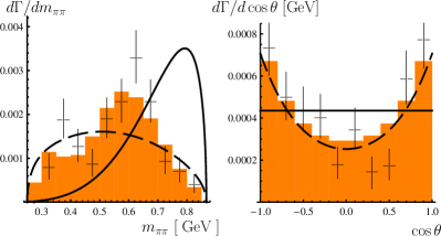
Figure 1: Dipion invariant mass ($m_{\pi\pi}$) distribution (left frame) and the $\cos\theta$ distribution (right frame) measured by Belle Abe:2007tk for the final state $\Upsilon(2S)\pi^{+}\pi^{-}$ (crosses), and the theoretical distributions based on this work (histograms). The solid and dashed lines show purely continuum contributions for different $\beta$.

Table 2: Fit values, yielding $F=0.86\pm 0.34$, $\beta=0.7\pm 0.3$ for the non-resonant contribution, and for the parameters entering in the resonant amplitude from $f_{0}(600)$ for the decay $Y_{b}\to\Upsilon(2S)\pi^{+}\pi^{-}$.

	$a_{f_{0}(i)}$	$F_{f_{0}(i)}$	$F_{f_{0}(i)}/F$	$\varphi_{f_{0}(i)}$ (rad.)
$f_{0}(600)$	$10.89\pm 2.4$	$4.19\pm 0.92$	$4.86\pm 2.18$	$2.76\pm 0.22$

The measured spectra (in $m_{\pi\pi}$ and $\cos\theta$) for the final state $\Upsilon(1S)\pi^{+}\pi^{-}$ from Belle Abe:2007tk are shown in Fig. 2 together with our theoretical distributions (histograms) obtained for the model in (9) having a $\chi^{2}/{\rm d.o.f.}\approx 5/5$ (obtained for the $m_{\pi\pi}$ spectrum in the upper left frame), with the fit parameters given in Table 3 yielding an integrated decay width of $\Gamma(Y_{b}\to\Upsilon(2S)\pi^{+}\pi^{-})=0.66$ MeV. The two curves in the upper frames show the shape of the continuum contribution based on (4), with the solid curves obtained for $\beta=0$ (as would be expected for the transition $\Upsilon(5S)\to\Upsilon(1S)\pi^{+}\pi^{-}$), and the dashed curves corresponding to the best-fit solution without the resonant contributions yielding $\beta\approx 0.3$ with $\chi^{2}/d.o.f\approx 65/11$ (obtained for the $m_{\pi\pi}$ spectrum). Both of them fail to describe the Belle data. In addition we show the contributions from the continuum plus a single resonance in the lower frames (solid curves: $f_{0}(600)$ with $\chi^{2}/d.o.f\approx 16/9$; dashed curves: $f_{0}(980)$ with $\chi^{2}/d.o.f\approx 30/9$; dotted curves: $f_{2}(1270)$ with $\chi^{2}/d.o.f\approx 33/9$). They also fail to describe the Belle data.

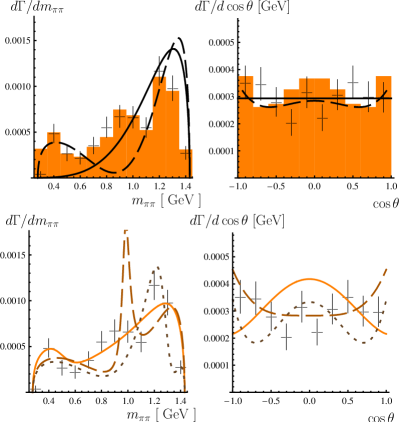
Figure 2: Upper Frames: The distributions measured by Belle Abe:2007tk for the final state $\Upsilon(1S)\pi^{+}\pi^{-}$ (crosses), and the theoretical distributions based on this work (histograms). The solid and dashed lines show purely continuum contributions for different $\beta$. Lower Frames: Contributions with continuum plus a single resonance (solid curves: $f_{0}(600)$; dashed curves: $f_{0}(980)$; dotted curves: $f_{2}(1270)$).

Table 3: Fit values, yielding $F=0.19\pm 0.03$, $\beta=0.54\pm 0.12$ for the non-resonant contribution, $a_{f_{2}(1270)}=0.5\pm 0.16$, $\varphi_{f_{2}(1270)}=3.33\pm 0.06$ for $f_{2}(1270)$, and for the parameters entering in the resonant amplitude from $f_{0}(600)$ and $f_{0}(980)$ for the decay $Y_{b}\to\Upsilon(1S)\pi^{+}\pi^{-}$.

	$a_{f_{0}(i)}$	$F_{f_{0}(i)}$	$F_{f_{0}(i)}/F$	$\varphi_{f_{0}(i)}$ (rad.)
$f_{0}(600)$	$3.6\pm 0.7$	$1.38\pm 0.27$	$7.34\pm 1.94$	$1.14\pm 0.14$
$f_{0}(980)$	$0.47\pm 0.02$	$1.02\pm 0.04$	$5.42\pm 1.0$	$4.12\pm 0.3$

We also remark that using the fits of the data for the decay $Y_{b}\to\Upsilon(1S)\pi^{+}\pi^{-}$ presented here, we are able to explain the decay width for the decay $Y_{b}\to\Upsilon(1S)K^{+}K^{-}$, measured by Belle Abe:2007tk . The decay is anticipated to be strongly dominated by the $0^{++}$ tetraquark state $f_{0}(980)$. Details will be published elsewhere.

Summarizing, we have argued here that the decays $Y_{b}\to\Upsilon(1S,2S)\pi^{+}\pi^{-}$ are radically different than the similar dipion transitions measured in the $\Upsilon(4S)$ and lower mass Quarkonia. The dynamical model presented by us will be tested in great detail with improved data, which we expect in the near future from Belle.

We thankfully acknowledge helpful communications with the members of the Belle and BaBar collaborations and thank Alexander Parkhomenko for his comments. M.J.A. would like to thank DESY for the hospitality and ENSF, Trieste, for financial support.

References

(1)
K. F. Chen et al. [Belle Collaboration],
Phys. Rev. Lett. 100, 112001 (2008)
[arXiv:0710.2577 [hep-ex]];
I. Adachi et al. [Belle Collaboration],
arXiv:0808.2445 [hep-ex].
(2)
W. S. Hou,
Phys. Rev. D 74, 017504 (2006)
[arXiv:hep-ph/0606016];
Yu. A. Simonov,
JETP Lett. 87, 121 (2008)
[arXiv:0712.2197 [hep-ph]];
C. Meng and K. T. Chao,
Phys. Rev. D 78, 034022 (2008)
[arXiv:0805.0143 [hep-ph]];
M. Karliner and H. J. Lipkin,
arXiv:0802.0649 [hep-ph].
(3)
L. S. Brown and R. N. Cahn,
Phys. Rev. Lett. 35, 1 (1975);
M. B. Voloshin,
JETP Lett. 21, 347 (1975)
[Pisma Zh. Eksp. Teor. Fiz. 21, 733 (1975)];
V. A. Novikov and M. A. Shifman,
Z. Phys. C 8, 43 (1981);
Y. P. Kuang and T. M. Yan,
Phys. Rev. D 24, 2874 (1981).
(4)
K. Gottfried,
Phys. Rev. Lett. 40, 598 (1978).
(5)
For reviews, see Y. P. Kuang,
Front. Phys. China 1, 19 (2006)
[arXiv:hep-ph/0601044];
and M. B. Voloshin,
Prog. Part. Nucl. Phys. 61, 455 (2008)
[arXiv:0711.4556 [hep-ph]].
(6)
S. L. Olsen,
Nucl. Phys. A 827, 53C (2009)
[arXiv:0901.2371 [hep-ex]];
A. Zupanc [for the Belle Collaboration],
arXiv:0910.3404 [hep-ex].
(7)
A. Ali, C. Hambrock, I. Ahmed and M. J. Aslam,
Phys. Lett. B 684, 28 (2010)
[arXiv:0911.2787 [hep-ph]].
(8)
B. Aubert et al. [BaBar Collaboration],
Phys. Rev. Lett. 102, 012001 (2009)
[arXiv:0809.4120 [hep-ex]].
(9)
N. V. Drenska, R. Faccini and A. D. Polosa,
Phys. Lett. B 669, 160 (2008)
[arXiv:0807.0593 [hep-ph]].
(10)
R. L. Jaffe,
Phys. Rev. D 15, 281 (1977).
R. L. Jaffe and F. E. Low,
Phys. Rev. D 19, 2105 (1979);
R. L. Jaffe and F. Wilczek,
Phys. Rev. Lett. 91, 232003 (2003)
[arXiv:hep-ph/0307341].
(11)
C. Amsler et al. [Particle Data Group],
Phys. Lett. B 667, 1 (2008).
(12)
G. ’t Hooft, G. Isidori, L. Maiani, A. D. Polosa and V. Riquer,
Phys. Lett. B 662, 424 (2008)
[arXiv:0801.2288 [hep-ph]].
(13)
L. Maiani, F. Piccinini, A. D. Polosa and V. Riquer,
Phys. Rev. Lett. 93, 212002 (2004)
[arXiv:hep-ph/0407017];
A. H. Fariborz, R. Jora and J. Schechter,
Phys. Rev. D 77, 094004 (2008)
[arXiv:0801.2552 [hep-ph]].
(14)
A. Sokolov et al. [Belle Collaboration],
Phys. Rev. D 79, 051103 (2009)
[arXiv:0901.1431 [hep-ex]].
(15)
I. Caprini, G. Colangelo and H. Leutwyler,
Phys. Rev. Lett. 96, 132001 (2006)
[arXiv:hep-ph/0512364].
(16)
E. M. Aitala et al. [E791 Collaboration],
Phys. Rev. Lett. 86, 770 (2001)
[arXiv:hep-ex/0007028].
(17)
S. Uehara et al. [Belle Collaboration],
Phys. Rev. D 78, 052004 (2008)
[arXiv:0810.0655 [hep-ex]].