Proposed Laboratory Search for Dark Energy

Abstract

The discovery of the accelerating universe indicates strongly the presence of a scalar field which is not only expected to solve today’s version of the cosmological constant problem, or the fine-tuning and the coincidence problems, but also provides a way to understand dark energy. It has also been shown that Jordan’s scalar-tensor theory is now going to be re-discovered in the new lights. In this letter we propose a way to search for the extremely light scalar field by means of a laboratory experiment using the low-energy photon-photon interactions with the quasi-parallel incident beam.

The discovery of the accelerating universe requires us finally to accept a nonzero cosmological constant, which is, however, smaller than the unification-oriented theoretical expectation by as much as 120 orders of magnitude exp , known widely as the fine-tuning problem, a part of today’s version of the cosmological constant problem. It seems highly remarkable to find that this fine-tuning is evaded naturally on the basis of the scalar-tensor theory (STT) invented first by Jordan jordan and now rediscovered with certain new ingredients included, to implement the scenario of a decaying cosmological constant, $\Lambda_{\rm obs}\sim t^{-2}$. The age of the universe $t_{0}=1.37\times 10^{10}{\rm y}$ is re-expressed by $\sim 10^{60}$ in the reduced Planckian units with $c=\hbar=M_{\rm P}(=(8\pi G)^{-1/2})=1$, providing us with an immediate derivation of $\Lambda_{\rm obs}\sim 10^{-120}$, or today’s $\Lambda$ is small simply because we are old cosmologically cup ; ipmurio .

The scalar field, denoted by $\sigma$, in STT is then expected to fill up nearly 3/4 of the entire cosmological energy exp , known as dark energy (DE). Searching for this crucial as well as major constituent of the universe by means of laboratory experiments deserves serious efforts. As we also point out, $\sigma$ is likely massive unlike authentic vector and tensor gauge fields. According to a simple assumption on the self-energy due to the loops of ordinary microscopic fields, we suggested an approximate relation $m_{\sigma}\sim m_{\rm q}M_{\rm ssb}/M_{\rm P}\sim 10^{-9}{\rm eV}$, in terms of the $u,d$ quark masses, the supersymmetry-breaking mass-scale and the Planck mass, respectively nat ; cup . This also corresponds to a macroscopic distance $m_{\sigma}^{-1}\sim 100{\rm m}$, though we allow for the latitude of a few orders of magnitude.

Past searches for the scalar force of this kind have been plagued by its matter coupling basically as weak as gravity wepv , inevitably with heavy and huge objects. This blockade can be removed, however, by appreciating that the scattering amplitude in which $\sigma$ occurs as a resonance reaches a maximum independent of the interaction strength, but with a concomitant narrow width. Also a resonance as light as above might be realized only by means of low-energy photon-photon scattering, unless, as required by the weak equivalence principle (WEP) yfms , $\sigma$ is totally decoupled from the photons. Through detailed analyses of the two-photon systems, we propose a novel type of laboratory experiments providing a glimpse of DE, anticipating an added building block $\sigma$ in the extended theory living with the accelerating universe. For other theoretical details we suppress, see our references cup ; ipmurio ; ptpkmyf .

For the reasons to be explained shortly, we prefer a special coordinate frame, as shown in Fig.1, in which two photons labeled by 1 and 2 sharing the same frequency are incident nearly parallel to each other, making an angle $\vartheta$ with a common central line along the $z$ axis. We define the $zx$ plane formed by $\vec{p}_{1}$ and $\vec{p}_{2}$. The components of the 4-momenta of the photons are given by $p_{1}=(\omega\sin\vartheta,0,\omega\cos\vartheta;\omega)$ and the same for $p_{2}$ but with the sign of $\vartheta$ reversed, and $p_{3}=(\omega_{3}\sin\theta_{3},0,\omega_{3}\cos\theta_{3};\omega_{3})$ and $p_{4}$ with $\omega_{3},\theta_{3}$ replaced by $\omega_{4},-\theta_{4}$, respectively.

The outgoing photons are assumed to be in the same $zx$ plane, to be convenient particularly in the $s$-channel reaction, showing an axial symmetry with respect to the $z$ axis. The angles $\theta_{3}$ and $\theta_{4}$, both positive $<\pi$, are defined also as shown in Fig.1. This coordinate frame can be transformed from the conventional CM frame for the head-on collision in the $x$ direction by a Lorentz transformation with the relative velocity $\beta_{z}=\cos\vartheta$.

The conservation laws are

$$0\mbox{-axis}: \omega_{3}+\omega_{4}=2\omega,$$ (1)

$$z\mbox{-axis}: \omega_{3}\cos\theta_{3}+\omega_{4}\cos\theta_{4}=2\omega\cos\vartheta,$$ (2)

$$x\mbox{-axis}: \omega_{3}\sin\theta_{3}=\omega_{4}\sin\theta_{4}.$$ (3)

For a convenient ordering $0<\omega_{4}<\omega_{3}<2\omega$, we may choose $0<\theta_{3}<\vartheta<\theta_{4}<\pi$, without loss of generality. From (1)-(3) we derive $\sin\theta_{3}/\sin\theta_{4}=\sin^{2}\vartheta/W$ with $W=1-2\cos\vartheta\cos\theta_{4}+\cos^{2}\vartheta$.

The differential elastic scattering cross section favoring the higher photon energy $\omega_{3}$ is given by footnote1

$$\frac{d\sigma}{d\Omega_{3}}=\left(\frac{1}{8\pi\omega}\right)^{2}\sin^{-4}\vartheta\left(\frac{\omega_{3}}{2\omega}\right)^{2}|M|^{2},$$ (4)

where $M$ is the invariant amplitude, and $\omega_{3}=(\omega\sin^{2}\vartheta)/(1-\cos\vartheta\cos\theta_{3})$. For $\vartheta\ll 1$, we then derive the upshifted frequency $\omega_{3}\rightarrow 2\omega$, as $\theta_{3}\rightarrow 0$, a clear observational signature, also occurring in the extremely forward direction within the angle $\vartheta$.

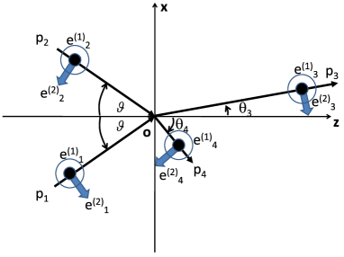
Figure 1: Definitions of kinematical variables.

The scalar field $\sigma$ may couple to the electromagnetic field with the effective interaction Lagrangian given by

$$-L_{\rm mx\sigma}=(1/4)BM_{\rm P}^{-1}F_{\mu\nu}F^{\mu\nu}\sigma,$$ (5)

where, due to the quantum-anomaly-type estimate, the constant $B$ is proportional to the fine-structure constant cup ; footnote2 . This interaction term, which has been discussed also from a phenomenological point of view bek , is WEP violating yfms , already in Brans-Dicke’s sense bd .

We find, for example,

$$<0\>|F_{\mu\nu}|\>p_{1},e_{1}^{(\beta)}\!>=i\left(p_{1\mu}e_{1\nu}^{(\beta)}-p_{1\nu}e_{1\mu}^{(\beta)}\right),$$ (6)

giving the two-photon decay rate of $\sigma$ with the mass $m_{\sigma}$;

$$\Gamma_{\sigma}=(16\pi)^{-1}\left(BM_{\rm P}^{-1}\right)^{2}m_{\sigma}^{3},$$ (7)

by assuming purely elastic scattering.

The polarization vectors are given by $\vec{e}_{i}^{\ (\beta)}$ with $i=1,\cdots,4$ for the photon labels, whereas $\beta=1,2$ are for the kind of linear polarization, also shown in Fig.1.

In the $s$-channel, the scalar field is exchanged between the pairs $(p_{1},p_{2})$ and $(p_{3},p_{4})$, thus giving the squared momentum of the scalar field $q_{s}^{2}=\left(p_{1}+p_{2}\right)^{2}=2\omega^{2}\left(\cos 2\vartheta-1\right)$ with the metric convention $(+++-)$.

With the type $\beta=1$ for all the photons we find footnote3 ;

$$M_{1111s}=-(BM_{\rm P}^{-1})^{2}\frac{\omega^{4}\left(\cos 2\vartheta-1\right)^{2}}{2\omega^{2}\left(\cos 2\vartheta-1\right)+m_{\sigma}^{2}},$$ (8)

where the denominator, denoted by ${\cal D}$, is the $\sigma$ propagator. We note $q_{s}$ is timelike, unlike $t$- and $u$-channels. We then make a replacement

$$m_{\sigma}^{2}\rightarrow\left(m_{\sigma}-i\Gamma_{\sigma}\right)^{2}\approx m^{2}_{\sigma}-2im_{\sigma}\Gamma_{\sigma}.$$ (9)

Substituting this into the denominator in (8), and expanding around $m_{\sigma}$, we obtain

$${\cal D}\approx-2\left(1-\cos 2\vartheta\right)\left(x+ia\right),\quad\mbox{with}\quad x=\omega^{2}-\omega_{r}^{2},$$ (10)

where

$$\omega_{r}^{2}=\frac{m_{\sigma}^{2}/2}{1-\cos 2\vartheta},\quad a=\frac{m_{\sigma}\Gamma_{\sigma}}{1-\cos 2\vartheta}.$$ (11)

Notice that both of $\omega_{r}^{2}$ and $a$ are enhanced as $\vartheta\rightarrow 0$.

Using (7) and (11) repeatedly, we finally obtain

$$|M_{1111s}|^{2}\approx(2\pi)^{2}\frac{a^{2}}{x^{2}+a^{2}},$$ (12)

from which we derive $|M_{1111s}|^{2}_{\omega=\omega_{r}}=(2\pi)^{2}$, a “large” value entirely free from being small due to the factor $M_{\rm P}^{-4}$. This is an aspect in the efforts to overcome the weak coupling of gravity, as alluded at the beginning. We may then ignore non-resonant terms in the $s$-channel and the whole contribution from the $t$- and $u$-channels. We still face the weak coupling in the extremely narrow width $a$, implied by $M_{\rm P}^{-2}$, in (7) and the second of (11).

To cope with this, we apply a process of averaging;

$$\overline{|M_{1111s}|^{2}}=\frac{1}{2\tilde{a}}\int_{-\tilde{a}}^{\tilde{a}}|M_{1111s}|^{2}dx=(4\pi)^{2}\eta^{-1}\frac{\pi}{2}\hat{\eta},$$ (13)

over the range $2\tilde{a}$ of $x\sim\omega^{2}$, where $\eta\equiv\tilde{a}/a$, also with $\hat{\eta}=(2/\pi)\tan^{-1}\eta$ reaching the maximum 1 for $\eta\rightarrow\infty$.

Substituting (13) into (4) we obtain

$$\overline{\left(\frac{d\sigma}{d\Omega_{3}}\right)}_{1111s}=\frac{\pi}{8\omega^{2}}\sin^{-4}\vartheta\left(\frac{\omega_{3}}{2\omega}\right)^{2}\eta^{-1}\hat{\eta}.$$ (14)

For later convenience, we parametrize $\eta$ by

$$\eta=\left(M_{\rm P}/m_{\sigma}\right)^{2-\gamma}.$$ (15)

We also derive $M_{1111s}=M_{2222s}=-M_{1122s}=-M_{2211s}$, for the only nonzero components. We are especially interested in $M_{1122s}$ from the experimental point of view as explained later.

In order to design experiments, we start with the resonance condition, the first of (11), by assuming $\vartheta\ll 1$,

$$m_{\sigma}/2\sim\vartheta\omega.$$ (16)

This indicates that experiments have the two adjustable handles for a given scalar mass scale. Since scanning $\vartheta$ would be much easier than scanning $\omega$, for the following argument, we assume fixing the incident energy and scanning $m_{\sigma}$ by changing $\vartheta$. We consider a case of the resonance condition with $\omega\sim 1$ eV (optical laser) and $\vartheta\sim 10^{-9}$ for $m_{\sigma}\sim 10^{-9}$ eV in what follows.

We find it useful to approximate $a$ in (11) by

$$a\sim\kappa(m_{\sigma}/(2\vartheta))^{2}\left(m_{\sigma}/M_{\rm P}\right)^{2},$$ (17)

where $\kappa\equiv B^{2}/4\pi\ll 1$. The integration range $\tilde{a}$ in (13) is thus re-expressed by using (15);

$$\tilde{a}=\eta a\sim\kappa\left(m_{\sigma}/(2\vartheta)\right)^{2}\left(m_{\sigma}/M_{\rm P}\right)^{\gamma}.$$ (18)

We first consider $\tilde{a}$ only due to the uncertainty in the incident angle $\delta\vartheta$ for a fixed $\omega^{2}$;

$$\tilde{a}=\omega^{2}-\omega_{r}^{2}\sim-\frac{\partial\omega_{r}^{2}}{\partial\vartheta}\delta\vartheta=\frac{1}{2}\left(\frac{m_{\sigma}}{\vartheta}\right)^{2}\frac{\delta\vartheta}{\vartheta}.$$ (19)

Combining this with (18) we obtain

$$\delta\vartheta/\vartheta\sim(\kappa/2)\left(m_{\sigma}/M_{\rm P}\right)^{\gamma}.$$ (20)

We emphasize that the resonance condition (16) defines not a point but a hyperbolic band in the $\vartheta-\omega$ plane given a finite $\delta\vartheta$. This implies that a deviation $\delta\omega$ from the nominal $\omega$ can satisfy the same resonance condition with a different $\vartheta$ within $\pm\delta\vartheta$. As far as $\delta\omega/\omega\ll\delta\vartheta/\vartheta$ is satisfied in a setup, we may ignore the effect of $\delta\omega$.

We introduce an experimental resolution $\epsilon$ defined by $\epsilon\equiv|\delta\vartheta/\vartheta|$, giving $\gamma\sim\ln(2\epsilon/\kappa)/\ln(m_{\sigma}/M_{\rm P})$, and hence

$$\eta\sim(M_{P}/m_{\sigma})^{2}(2\epsilon/\kappa),$$ (21)

due to (15). Substituting this into (14), we derive

$$\overline{\frac{d\sigma}{d\Omega_{3}}}\sim\frac{\pi}{8\omega^{2}}\vartheta^{-4}\left(\frac{m_{\sigma}}{M_{P}}\right)^{2}\left(\frac{\kappa}{2\epsilon}\right),$$ (22)

in the extremely forward direction. It is remarkable that the small $\vartheta\sim 10^{-9}$ produces a huge factor which nearly compensates $(m_{\sigma}/M_{P})\sim 10^{-36}$, leaving us with another $10^{-36}$ which can be taken care of by a sufficiently strong laser beam. In addition, thanks to the narrow forward peak, measuring $\omega_{3}\sim 2\omega$ frees us from measuring the angle $\theta_{3}$ directly to the demanding resolution $\sim 10^{-9}$.

In principle we can explore the entire mass range $m_{\sigma}<\pi\omega$ by using two crossing beams with small incident angles. Then we can directly measure the resonance curve in (16) by scanning both $\vartheta$ and $\omega$ to observe the resonance nature explicitly. For the smaller mass scale such as $m_{\sigma}\mbox{\raisebox{-3.00003pt}{$\;\stackrel{{\scriptstyle<}}{{\sim}}\;$}}10^{-9}$ eV, however, we must take the finite beam size due to the diffraction limit into account for controlling the small incident angle with realizable optical devices and a distance on the ground.

For this purpose, we now propose a conceptual experimental setup with one-beam focusing as illustrated in Fig.2. Incident photons from a Gaussian laser pulse linearly polarized to the state 11 are focused by the conceptual thin lens component into the diffraction limit with a reasonable focal length to satisfy the resonance condition. The quasi-parallel incident photons interact with each other around the focal point, from which photons 3 and 4 are emitted nearly in the opposite direction along the $z$ axis with $\omega_{3}\sim 2\omega$ and $\omega_{4}\sim 0$. The mirror with a dichroic nature is almost transparent to the non-interacting photons, while $\omega_{3}$ is reflected to the prism (equivalent to a group of dichroic mirrors) which selects $\omega_{3}$ among residual $\omega$ and sends it to the photon detector placed off the $z$ axis. This process is assisted by the polarization filter selecting the rotated state 22.

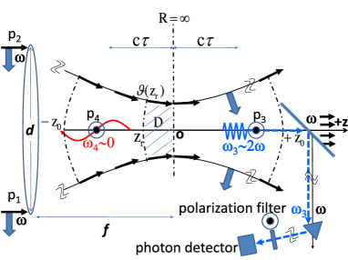
Figure 2: A conceptual experimental setup.

The electric field component in the Gaussian beam as a function of spatial coordinate $(x,y,z)$ is well-known Yariv ,

$$E\!\propto\!\frac{w_{0}}{w(z)}\exp\left(-i\!\left[\rule[-1.00006pt]{0.0pt}{10.00002pt}kz\!+\!\frac{kr^{2}}{2R(z)}-\phi(z)\right]-\frac{r^{2}}{w(z)^{2}}\right)\!,$$ (23)

where $k=2\pi/\lambda$ with wavelength $\lambda$, $r=\sqrt{x^{2}+y^{2}}$, $w_{0}$ being the minimum waist, while other definitions are curvature $R(z)=z(1+{z_{0}}^{2}/z^{2})$, phase $\phi(z)=\tan^{-1}(1+z/z_{0})$ and the waist $w(z)$ as a function of $z$;

$${w(z)}^{2}={w_{0}}^{2}(1+z^{2}/{z_{0}}^{2}),$$ (24)

with a parameter $z_{0}\equiv\pi{w_{0}}^{2}/\lambda$. We introduce the $F$-number with the focal length $f$ and the laser beam diameter $d$ defined by $F=2f/(\pi d)$. Then the beam waist at $z=0$ is given by $w_{0}=(d/2)(f/z_{0})/\sqrt{1+(f/z_{0})^{2}}\sim F\lambda$ for $f\ll z_{0}$ which is the case we are interested in and we focus on the diffraction limit in $|z|<z_{0}$ in what follows.

According to (23), curvature $R=\infty$ is exactly satisfied at $z=0$ with $\vartheta=0$. We may thus expect the resonance condition (16) to be met automatically somewhere in the region $-z_{0}<z<0$. The upper limit of the resonance angle $\vartheta(z_{r})$ on the same wavefront (equi-phase surface) can be estimated from (24) for $|z_{r}|\ll z_{0}$;

$$\vartheta(z_{r})\equiv\frac{w(z_{r})-w_{0}}{z_{r}}\sim\frac{w_{0}z_{r}}{2{z_{0}}^{2}}=\frac{1}{2\pi^{2}F^{3}}\frac{z_{r}}{\lambda}.$$ (25)

At any $z_{r}$, the incident angle between any combinations of two photons from the same wavefront varies between $0<\vartheta<\vartheta(z_{r})$. The mean $\vartheta$ of the two photons chosen randomly from the above range originating from a spherical wavefront is $\bar{\vartheta}\equiv(1/3)\vartheta(z_{r})$. It then follows that the experimental resolution cannot be $\epsilon\leq 2$ for any $z_{r}$. For $z_{r}\leq z<0$, called the domain $D$, on the other hand, the condition $0<\vartheta(z)<\vartheta(z_{r})$ is satisfied. We then find that $\epsilon\sim{\cal O}(1)$ can be assigned for the domain $D$ as the upper limit on the incident angular resolution.

Let us estimate effective luminosity in $D$. Suppose a Gaussian laser pulse with the duration time $\tau$ satisfying $c\tau\leq z_{0}$ with the light velocity $c$ enters $D$ from the left side with the average number of photons $\bar{N}$. The effective number of photons in $D$ which allows the use of the cross sections in (22) with $\epsilon\sim{\cal O}(1)$ is defined by $\bar{N}_{D}=|z_{r}|/(c\tau)\bar{N}$. The effective luminosity per transverse area inside the laser pulse in $D$ is expressed as

$${\cal L}=b\>C(\bar{N}_{D},2)/\left(\pi w^{2}(z_{r})\right)\sim\left(\pi F\omega\bar{\vartheta}/c^{2}\tau\right)\bar{N}^{2},$$ (26)

where $C(\bar{N}_{D},2)\approx\bar{N}_{D}^{2}/2$, while $b$ is for how many domains with fixed $\epsilon$ are contained in the incident pulse with the total length $c\tau$, hence $b=c\tau/|z_{r}|$ with $z_{r}$ defined by $\vartheta(z_{r})$ in (25), with further approximation $w(z_{r})\sim w_{0}$.

Multiplying (22) times $c^{2}$ by (26), we obtain the differential yield footnote4 ,

$$\frac{d{\cal Y}}{d\Omega_{3}}=\frac{\pi^{2}}{16}\bar{\vartheta}^{-3}(F/\omega\tau)(m_{\sigma}/M_{P})^{2}(\kappa/\epsilon)\bar{N}^{2},$$ (27)

per pulse rather than per unit time, since (26) includes the effect from the entire pulse. We then define $\bar{N}_{1}$ by

$$\bar{N}_{1}=\frac{4}{\pi}\sqrt{\frac{\epsilon\tau\omega\bar{\vartheta}^{3}}{\kappa F}}(M_{P}/m_{\sigma}),$$ (28)

for $d{\cal Y}/d\Omega_{3}={\cal O}(1)$, or a single photon per pulse focusing.

Although this proposal applies both to CW and pulsed laser systems by optimizing $F/\omega\tau$ and $\bar{N}$, we here estimate a rate for a short laser pulse system based on (28) with $\epsilon={\cal O}(1)$ and the physical parameters: $\bar{\vartheta}\sim 10^{-9},\>\omega\sim 1$ eV with $\kappa\sim 10^{-4}$ and $M_{P}\sim 10^{27}$ eV. For $F\sim 10^{2}$ and $c\tau\sim 1({\rm eV})^{-1}$ with $\tau\sim 4$ fs, we find $\bar{N}_{1}=10^{23}\sim 10$ kJ per pulse focusing footnote4 . Since the conceptual lens component must have a reasonable aperture size to keep the incident power density below the damage threshold, the dichroic mirror is assumed to be located at the symmetric position from the focal point at shortest. The solid angle is then estimated to be $d\Omega_{3}\sim F^{-2}\sim 10^{-4}$. For a 10 Hz repetition rate the signal rate is $10^{-3}$ Hz assuming the perfect detection efficiency for $\omega_{3}$ after the mirror.

A major instrumental background for the doubled frequency appears to come from the second harmonic generation (SHG) due to gas-solid interfaces with the centrosymmetry broken maximally. Even from the maximal estimate $\sim 10^{13}$W/cm² for a typical damage threshold, we find a negligible amount of $10^{-10}$ SHG photons from a 1m² aperture size with a 10 fs irradiation, if the optical components are housed in a vacuum containing $10^{10}$ atoms/cm³ ($\sim 10^{-5}$ Pa) SHG .

As a dominant physical background we expect the lowest-order QED photon-photon scattering, with the forward cross section, $\sim(\alpha^{2}/m_{e}^{4})^{2}\omega^{6}\vartheta^{4}$ XsecQED . This turns out to be smaller than (22) by 50 orders of magnitude for the above parameter values, indicating the QED contribution to be totally negligible. The resonance effects due to a pseudoscalar-field exchange from axion-like particles can also be suppressed if the initial photon polarizations are all in parallel as in our conceptual design.

In view of these estimates of the suppressed backgrounds, instrumental and physical, our proposal is expected to be a basis for realizing actual experiments by respecting the novel ideas in overwhelming the weak gravitational coupling by such non-gravitational effects like the small incident angle and the high laser intensity.

- (1) A.G. Riess, et al., Astron. J. 116 (1998), 1009, S. Perlmutter, et al., Nature 391, (1998), 51.
- (2) P. Jordan, Schwerkraft und Weltall (Friedrich Vieweg und Sohn, Brunschweig, 1955).
- (3) Y. Fujii and K. Maeda, The Scalar-Tensor Theory of Gravitation (Cambridge Univ. Press, 2003).
- (4) Y. Fujii, arXiv:0908.4324 [astro-ph.CO]. Y. Fujii, Proc. IAU 2009 JD9, 03-14 Aug. 2009, Mem. S.A.It. Vol. 75, 282, arXiv:0910.5090 [astro-ph.CO].
- (5) Y. Fujii, Nature Phys. Sci. 234 (1971), 5.
- (6) See, for example, Figures; 2.13, 4.16-17 in E. Fischbach and C. Talmadge, The Search for Non-Newtonian Gravity (AIP Press, Springer-Verlag, N.Y., 1998).
- (7) Y. Fujii and M. Sasaki, Phys. Rev. D75 (2007), 064028.
- (8) Y. Fujii, Prog. Theor. Phys. 118 (2007), 983. K. Maeda and Y. Fujii, Phys. Rev. D79 (2009), 084026.
- (9) The factor comes, for example, from the massless limit of the denominator of (3.78) in W. Greiner and J. Reinhardt, Quantum Electrodynamics (Springer 1994).
- (10) We have , which is times as large as the coefficient in (6.194) in cup , because of slightly different processes and using half-spin fermions instead of spinless fields in a toy model in the loop.
- (11) J. D. Bekestein, Phys. Rev. D25 (1982), 1527.
- (12) C. Brans and R. H. Dicke, Phys. Rev. 124 (1961), 925.
- (13) The four digits in the subscript are for arranged from left to right according to the photon labels, 1-4.
- (14) Am non Yariv, Optical Electronics in Modern Communications (Oxford University Press, Inc. 1997).
- (15) We point out the potential importance of the possible coherent amplification of the scattering amplitude over the entire laser volume which is covered by the long force-range of the scalar field, with likely a huge effect of multiplication by another factor on the cross section SMITH_COHERENT .
- (16) P. F. Smith, IL NUOVO CIMENTO 83A (1984), 263.
- (17) V. G. Bordo, Optics Communications 132 (1996), 62-72.
- (18) See p.183 in W.Dittrich and H.Gies, Probing the Quantum Vacuum (Springer 2007).