Oscillatory Dynamics in Rock-Paper-Scissors Games with Mutations

Abstract
We study the oscillatory dynamics in the generic three-species rock-paper-scissors games with mutations. In the mean-field limit, different behaviors are found: (a) for high mutation rate, there is a stable interior fixed point with coexistence of all species; (b) for low mutation rates, there is a region of the parameter space characterized by a limit cycle resulting from a Hopf bifurcation; (c) in the absence of mutations, there is a region where heteroclinic cycles yield oscillations of large amplitude (not robust against noise). After a discussion on the main properties of the mean-field dynamics, we investigate the stochastic version of the model within an individual-based formulation. Demographic fluctuations are therefore naturally accounted and their effects are studied using a diffusion theory complemented by numerical simulations. It is thus shown that persistent erratic oscillations (quasi-cycles) of large amplitude emerge from a noise-induced resonance phenomenon. We also analytically and numerically compute the average escape time necessary to reach a (quasi-)cycle on which the system oscillates at a given amplitude.

Keywords: Population Dynamics; Fluctuations and Demographic Noise; Evolutionary Game Theory; Co-evolution, Cyclic Dominance and Biodiversity; Cycles and Quasi-Cycles.

1 Introduction

Understanding the mechanisms allowing co-evolution and the maintenance of biodiversity is a key issue in theoretical biology and ecology (May (1974); Michod (2000); Hubbell (2001); Haken (2002); Murray (2002); Neal (2004)). In this context, cyclic dominance has been identified as a potential mechanism that helps promote species diversity (Durrett and Levin (1994, 1997); Gilg et al. (2001); Kerr et al. (2002); Czárán et al. (2002)) and is naturally investigated in the framework of evolutionary game theory (EGT) (Maynard Smith (1982); Hofbauer and Sigmund (1998); Nowak (2006); Szabó and Fath (2007)). The emergence of oscillatory (or quasi-oscillatory) behavior is one of the most appealing and debated phenomena that often characterizes co-evolution in population dynamics (Sinervo and Lively (1996); Zamudio and Sinervo (2000); Kerr et al. (2002); Kirkup and Riley (2004); Dawkins (1976); Bastolla et al. (2002); Hauert et al. (2002); Mobilia et al. (2007)). Oscillatory dynamics has notably been observed in predator-prey and host-pathogen systems (Anderson and May (1986, 1991); Berryman (2002); Turchin (2003)), as well as in genetic networks (Elowitz and Leibler (2000)). Here, we study the oscillatory dynamics of rock-paper-scissors games with mutations and demonstrate that this favors the long-lasting co-evolution of all species. Rock-paper-scissors games (RPS) –in which rock crushes scissors, scissors cut paper, and paper wraps rock (Hofbauer and Sigmund (1998); Nowak (2006); Szabó and Fath (2007))– have emerged as paradigmatic mathematical models in EGT to describe the cyclic competition in ecosystems (Tainaka (1994); May and Leonard (1975); Szabó and Szolnoki (2002); Reichenbach et al. (2006, 2007a, 2008b); Perc et al. (2007); Claussen and Traulsen (2008); Peltomäki and Alava (2008); Berr et al. (2009)). In addition to their theoretical relevance, and in spite of their apparent simplicity, it has been argued that the RPS model and the like can help understand the co-evolutionary dynamics of different biological systems, such as the cyclic dominance observed in some communities of lizards (Sinervo and Lively (1996); Zamudio and Sinervo (2000)). Another popular example is the cyclic competition between three strains of E.coli (Kerr et al. (2002)). In this case, it has been found that cyclic dominance yields coexistence of all species in a spatial setting, while in a well-mixed (homogeneous) environment two species go extinct after a short transient. Naturally therefore, the mathematical properties of the RPS model and of its variants have recently attracted much interest. In an EGT setting, the RPS dynamics is classically described in terms of the replicator equations (REs) that is a set of deterministic rate equations (see below) (Hofbauer and Sigmund (1998); Nowak (2006); Szabó and Fath (2007)). The latter essentially predict two types of behavior for the RPS dynamics: there is either the stable coexistence of all species, or oscillations of large amplitudes with each species almost taking over the entire system in turn and then suddenly almost going extinct. As population dynamics always involves a finite (yet, often large) number of discrete entities, it is necessary to take the effects of noise into account and understand its influence on the ensuing nonlinear dynamics (Nisbet and Gurney (1982); Ewens (2004)). In the context of population models, demographic stochasticity (i.e. intrinsic noise) is naturally accounted by adopting an ‘individual-based’ modeling. The stochastic dynamics is thus implemented in terms of random birth and death events, like in the Moran process (Moran (1958); Nowak (2006)). Recently, individual-based modeling has been extensively used to study the stochastic RPS dynamics. In fact, a large body of research has been concerned with spatially-extended systems and the influence of the species’ movement on the emerging noisy patterns (Tainaka (1994); Reichenbach et al. (2007a, b, 2008b); Peltomäki and Alava (2008)). On the other hand, for systems with homogeneous (well-mixed) populations, it is well established that intrinsic noise drastically alters the replicator dynamics and recent studies have focused on the mean time and probability of extinction of two species (Reichenbach et al. (2006); Claussen and Traulsen (2008); Berr et al. (2009)).

In addition to selection and reproduction, a third basic evolutionary mechanism is mutation. The latter is generally regarded as providing the advantageous traits that survive and multiply in offsprings (Neal (2004); Michod (2000)). Also, from a behavioral perspective, it is recognized that agents never behave perfectly rationally and it is sensible to assume that individuals can switch their strategies and therefore undergo mutations (Antal et al (2009); Szabó and Fath (2007)). While selection and reproduction are present in the RPS models considered in Refs. (Tainaka (1994); Szabó and Szolnoki (2002); Reichenbach et al. (2006, 2007a); Perc et al. (2007); Claussen and Traulsen (2008); Reichenbach et al. (2007b, 2008b); Peltomäki and Alava (2008); Berr et al. (2009)), the latter do not account for mutations. Here, we study the oscillatory dynamics of RPS games with mutations and show that the possibility to switch from one strategy (species) to another with a small transition rate yields novel oscillatory dynamics and favors long-term coexistence. For population of finite size, we discuss the effect of demographic noise on the dynamics and show that it induces persistent (quasi-)cyclic behavior characterized by sustained erratic oscillations of non-vanishing amplitude.

The remainder of the paper is organized along the following lines. In the next section we introduce the generic RPS model with mutations (RPSM) and describe its dynamics in the mean-field limit. The (generalized) REs are studied in Section 3, where the bifurcation diagram is obtained (Sec. 3.1) and a new region of the parameter space characterized by a Hopf bifurcation is identified. The main properties of the resulting limit cycle are briefly discussed in Sec. 3.2. Section 4 is dedicated to the stochastic dynamics of the model RPSM in terms of an individual-based formulation. In particular, we show that demographic noise can cause quasi-cyclic behavior with persistent oscillations of large amplitude (Sec. 4.1), and allow to escape – after a characteristic time that is computed – from the coexistence fixed point and reach a given (quasi-)cycle (Sec. 4.2). In the final section, we summarize and discuss our results.

2 Rock-Paper-Scissors with Mutations

In their essence, all variants of the RPS game aim at describing the co-evolutionary dynamics of three species, say $A,B$ and $C$, in cyclic competition. In this setting, as in the children’s game, ‘rock’ (here species $A$) crushes the ‘scissors’ (species $B$), and ‘paper’ (species $C$) wraps the ‘rock’, and ‘scissors’ cut the ‘paper’. We therefore say that $A$ dominates over $C$, which outcompetes $B$, which outgrows $A$ and thus closes the cycle. In EGT, the interactions are specified in terms of a payoff matrix ${\cal P}$. Generically, the cyclic dominance of RPS games is captured by the following payoff matrix (Hofbauer and Sigmund (1998); Nowak (2006); Szabó and Fath (2007)), where $\epsilon>0$:

${\cal P}=$ vs Rock $(A)$ Paper $(B)$ Scissors $(C)$ Rock $(A)$ $0$ $-\epsilon$ $1$ Paper $(B)$ $1$ $0$ $-\epsilon$ Scissors $(C)$ $-\epsilon$ 1 0

According to this matrix, when a pair of $A$ and $B$ players interacts, the former gets a negative payoff $-\epsilon$ while the latter gets a payoff $1$. In this case, $A$ is dominated by $B$ and its loss is less than $B$’s gain when $0<\epsilon<1$, whereas $B$’s gain is higher than $A$’s loss when $\epsilon>1$. In the same way, $C$’s dominate over $B$’s and the latter prevail against $A$’s, and thus the model exhibits cyclic dominance. In all pairwise interactions, the dominant individual gets a payoff $1$, whereas the dominated one obtain a negative payoff $-\epsilon$. Therefore, the parameter $\epsilon$ allows to introduce an asymmetry (when $\epsilon\neq 1$) in the interactions. When $\epsilon=1$, one of the player loses what the other gains and this perfect balance corresponds to a zero-sum game.

In EGT, one often considers homogeneous (well-mixed) populations of $N$ individuals, with $N\to\infty$. In this mean-field limit, the dynamics is usually specified in terms of the REs for the densities (or relative abundances) $a(t),b(t)$ and $c(t)$ of species $A,B$ and $C$, respectively (Hofbauer and Sigmund (1998); Nowak (2006); Szabó and Fath (2007)). Introducing the vector ${\bm{s}}(t)$, whose components $s_{i}$, with $\;i\in(A,B,C)$, are $s_{A}\equiv a(t),s_{B}\equiv b(t)$ and $s_{C}\equiv c(t)$, the REs read $\dot{s_{i}}=s_{i}[({\cal P}{\bm{s}})_{i}-{\bm{s}}.{\cal P}{\bm{s}}]=s_{i}[\pi_{i}-\bar{\pi}]$, where the dot stands for the time derivative. The important notion of average payoff (per individual) of species $i$, $\pi_{i}$, has been introduced in terms of the payoff matrix as a linear function of the relative abundances: $\pi_{i}\equiv({\cal P}{\bm{s}})_{i}$, whereas $\bar{\pi}={\bm{s}}.{\cal P}{\bm{s}}=\sum_{i}s_{i}\pi_{i}$ denotes the population’s mean payoff (Hofbauer and Sigmund (1998); Nowak (2006); Szabó and Fath (2007)). In addition to the above processes of selection/reproduction, we introduce a third evolutionary mechanism that allows each individual to mutate from one species to another with rate $\mu$:

$$A\stackrel{{\scriptstyle\mu}}{{\longrightarrow}}\begin{cases}B\\ C\end{cases}\,,\quad B\stackrel{{\scriptstyle\mu}}{{\longrightarrow}}\begin{cases}A\\ C\end{cases}\,,\quad C\stackrel{{\scriptstyle\mu}}{{\longrightarrow}}\begin{cases}A\\ B\end{cases}.$$ (1)

In this setting, the natural generalization of the replicator equations for the model under consideration is $\dot{s}_{i}=s_{i}[\pi_{i}-\bar{\pi}]+\mu(1-3s_{i}),$ with $\pi_{A}=c-\epsilon b,\;\pi_{B}=a-\epsilon c,\;\pi_{C}=b-\epsilon a$ and $\bar{\pi}=(1-\epsilon)(ab+bc+ac)$. The latter are studied in the next sections.

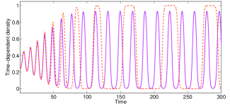
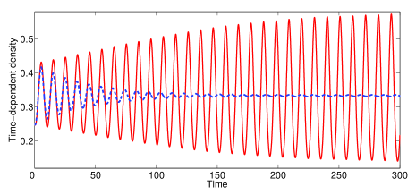
Figure 1: (Color online). Typical plots of the time-dependent density (relative abundance) $a(t)$ of species $A$, obtained from Eqs. (3) for $\epsilon=1.225$ and different values of $\mu$ (with $a(0)=0.25,b(0)=0.40$). Here, $\mu_{c}=0.0125$ (see text). Left: In the absence of mutation rate ($\mu=0,\lambda=0.0375$), the fixed point ${\bm{s}}^{*}$ is unstable and the density (brown, dashed) jumps from $0$ to $1$. For very low values of the mutation rate, here $\mu=0.001$ ($\lambda=0.0345$), ${\bm{s}}^{*}$ is also unstable and $a(t)$ oscillates regularly (magenta, solid) with an amplitude that approaches the extreme values $0$ and $1$, but with a much shorter period than in the case $\mu=0$. Right: For $\mu=0.01$ ($\lambda=0.0075$), the fixed point ${\bm{s}}^{*}$ is still unstable and $a(t)$ oscillates regularly about $a^{*}=1/3$ (red, solid), with a period $T\approx 10$. When $\mu=0.02>\mu_{c}$ ($\lambda=-0.0225$), the densities exhibit exponentially damped oscillations and converge towards the fixed point value $1/3$ (blue, dashed).

3 The Rate Equations

Here, we consider the dynamics of the model RPSM in the mean-field limit, where $N\to\infty$. When the population is well-mixed (homogeneous) and every pair of random individuals has the same probability to interact, demographic noise can be neglected and the system’s dynamics is aptly described by the rate equations

$$\dot{a} = a\left[c-\epsilon b-(1-\epsilon)\left\{ab+bc+ac\right\}\right]+\mu(1-3a)$$

$$\dot{b} = b\left[a-\epsilon c-(1-\epsilon)\left\{ab+bc+ac\right\}\right]+\mu(1-3b)$$ (2)

$$\dot{c} = c\left[b-\epsilon a-(1-\epsilon)\left\{ab+bc+ac\right\}\right]+\mu(1-3c)$$

As the system is comprised of three species, the sum of the population density is conserved, i.e. $a(t)+b(t)+c(t)=1$. Clearly, this constant of motion allows, say, to set $c(t)=1-a(t)-b(t)$ and reduces (3) to a system with only two variables (here, $a(t)$ and $b(t)$). Thereafter, the properties of these equations are studied and it will be shown that mutations yield a new region in the parameter space characterized by a stable limit cycle.

It is known that in the absence of mutations ($\mu=0$) the REs admit one interior fixed point, ${\bm{s}^{*}}=(a^{*},b^{*},c^{*})=(1/3,1/3,1/3)$, and three absorbing states ($(1,0,0)$, $(0,1,0)$ and $(0,0,1)$). The resulting cyclic dynamics gives rise to three kinds of behavior (Hofbauer and Sigmund (1998); Nowak (2006); Szabó and Fath (2007)): (i) When $\epsilon<1$, ${\bm{s}^{*}}$ is the system’s only attractor, it is globally stable and the trajectories in the phase portrait spiral towards it (${\bm{s}^{*}}$ is a focus). (ii) When $\epsilon>1$, the interior rest point ${\bm{s}^{*}}$ becomes unstable and the flows in the phase portrait form a heteroclinic cycle connecting each of the absorbing fixed points (saddles) at the boundary of the phase portrait. Clearly, as any fluctuations cause the rapid extinction of two species, the resulting oscillations are non-robust (May and Leonard (1975); Durrett and Levin (1994)). (iii) When $\epsilon=1$, $\bar{\pi}$ vanishes (zero-sum game) and the interior rest point ${\bm{s}^{*}}$ is marginally stable (center). In this case, the quantity $a(t)b(t)c(t)$ is a constant of motion and the trajectories in the phase portrait form closed orbits around ${\bm{s}^{*}}$, set by the initial conditions and not robust against noise (see e.g. (Reichenbach et al. (2006))).

In the presence of mutations, solving Eqs. (3) with $\dot{a}=\dot{b}=\dot{c}=0$, one finds that ${\bm{s}^{*}}=(1/3,1/3,1/3)$ is the only (interior) fixed point of the system. The absence of absorbing points when $\mu>0$ indicates that the model under consideration does not yield heteroclinic cycles. In fact, as shown below, in the presence of small mutation rate the heteroclinic cycles are replaced by stable cycles resulting from a Hopf bifurcation (region (b) in Fig. 2) and yield persistent oscillatory dynamics of all species, which is a feature of biological relevance.

3.1 Linear stability analysis

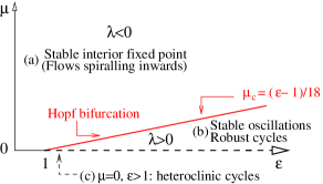
Figure 2: (Color online). Bifurcation diagram in the parameter space of the (deterministic) model RPSM. The regions (a) and (b) are separated by the critical mutation rate $\mu_{c}=(\epsilon-1)/18>0$. In region (a), $\mu>\mu_{c}$ for $\epsilon>1$ and $\mu\geq 0$ for $\epsilon\leq 1$, ${\bm{s}}^{*}$ is a stable focus. Below the line $\mu_{c}(\epsilon)$, in region (b) where $0<\mu<\mu_{c}$, the system undergoes a Hopf bifurcation (at $\mu=\mu_{c}$) and the dynamics is characterized by a limit cycle and stable oscillations. In region (c), where $\mu=0$ (no mutations) and $\epsilon>1$ (dashed line), the REs (3) yield heteroclinic cycles along with periodic oscillations that are unstable against demographic fluctuations.

To investigate the properties of REs (3), it is useful to introduce the variables ${\bm{x}}=(x_{A},x_{B})$:

$$x_{A}=a-a^{*}=a-\frac{1}{3}\quad\text{and}\quad x_{B}=b-b^{*}=b-\frac{1}{3},$$ (3)

which measure the deviations from the interior fixed point ${\bm{s}^{*}}$. We notice that $x_{C}=c-c^{*}=-(x_{A}+x_{B})$. As a first step to gain some insight into the dynamics described by (3), it is useful to perform a linear stability analysis. To linear order in terms of ${\bm{x}}=(x_{A},x_{B})$), the REs (3) can be rewritten as $\dot{\bm{x}}=\mathcal{A}({\bm{s}^{*}}){\bm{x}}$, where $\mathcal{A}({\bm{s}^{*}})$ is the Jacobian matrix at ${\bm{s}^{*}}$ whose (complex conjugate) eigenvalues which are $\lambda_{\pm}=\lambda\pm i\,\omega_{0}$, with

$$\lambda=\frac{\epsilon-1}{6}-3\mu\quad\text{and}\quad\omega_{0}=\frac{1+\epsilon}{2\sqrt{3}}.$$ (4)

General results therefore guarantee that ${\bm{s}}^{*}$ is (globally) stable when $\lambda<0$, i.e. for $18\mu>\epsilon-1$, whereas ${\bm{s}}^{*}$ is unstable when $\lambda>0$ and a Hopf bifurcation occurs at the critical value $\mu=\mu_{c}(\epsilon)$ and $\epsilon>1$ is kept fixed, with

$$\mu_{c}\equiv\frac{\epsilon-1}{18}>0,$$ (5)

The bifurcation diagram of the model is thus summarized in Fig. 2. Such a diagram clearly illustrates the effect of mutations and is characterized by three regions. In region (b), where $0<\mu<\mu_{c}$, ${\bm{s}}^{*}$ is unstable and there is a Hopf bifurcation at $\mu=\mu_{c}$ (as demonstrated below) which leads to the coexistence of all species with stable oscillations of their densities (right panel of Fig. 1, red/solid). On the other hand, in region (a), where $\mu>\begin{cases}\mu_{c}&\;\text{, for}\quad\epsilon>1\\ 0&\;\text{, for}\quad\epsilon\leq 1\end{cases},$ i.e. when $\lambda<0$, the densities are exponentially damped, with an amplitude ${\rm A}_{\rm amp}(t)\approx e^{-|\lambda|t}$ that vanishes near $\bm{s}^{*}$ (right panel of Fig. 1, blue/dashed). In the absence of mutations and when $\epsilon>1$ (region (c) in Fig. 2), one recovers the scenario characterized by heteroclinic cycles (left panel of Fig. 1, brown/dashed). In this case, the density of each species oscillates, with a large period, between the extreme values $0$ (absence of a given species) and $1$ (presence of only one species). These oscillations are not robust against demographic noise: chance fluctuations will unavoidably and quickly drive the system into an absorbing state. When $\lambda=0$, the fixed point ${\bm{s}}^{*}$ is a center and its stability is determined by nonlinear terms. Below, we shall consider the dynamics to third order about ${\bm{s}}^{*}$ and show that it is stable when $\lambda=0$ and $\mu>0$. Only in the marginal case $\lambda=\mu=0$, ${\bm{s}}^{*}$ is marginally stable (see e.g. (Reichenbach et al. (2006))).

3.2 Hopf bifurcation and limit cycle

As qualitatively discussed above, at mean-field level, the most interesting effect of mutations is the emergence of robust oscillatory behavior (stable limit cycle) resulting from a Hopf bifurcation occurring at low mutation rates (right panel of Fig. 1, red/solid). To study the properties of the resulting limit cycle and take advantage of the system’s symmetry around ${\bm{s}}^{*}$, it is convenient to perform the linear transformation ${\bm{x}}\to{\mathcal{S}}{\bm{x}}\equiv{\bm{y}}$, where ${\mathcal{S}}=\begin{pmatrix}1&\frac{1}{2}\\ 0&\frac{\sqrt{3}}{2}\end{pmatrix}$. As well known from bifurcation theory (Wiggins (1990); Grimshaw (1994)), one then Taylor expands the REs (expressed in the variables ${\bm{y}}={\mathcal{S}}{\bm{x}}$) to third-order around ${\bm{s}}^{*}$ and recasts the resulting rate equations into the Hopf bifurcation normal form. Hence, in polar coordinates $(r,\theta)$, the normal form of the REs (truncated to third order) reads

$$\dot{r} = r(\lambda+\beta r^{2})$$

$$\dot{\theta} = \omega_{0}-\alpha r^{2},$$ (6)

where

$$\alpha = \frac{18\omega_{0}(1+2\sqrt{3}\omega_{0})}{7(1+\epsilon^{2})+\epsilon(13-9\mu)+9\mu(1+9\mu)}$$ (7)

$$\beta = 1-\epsilon-\left(\frac{6\lambda(1+2\epsilon\sqrt{3}\omega_{0})}{7(1+\epsilon^{2})+\epsilon(13-9\mu)+9\mu(1+9\mu)}\right).$$

One readily recognizes that (3.2) yield a supercritical Hopf bifurcation when $\lambda>0$ (for $0<\mu<\mu_{c}(\epsilon)$). In fact, the parameter $\beta$ is the first Lyapunov coefficient and is negative when $\lambda>0$ and the mutation rate $\mu$ is small (i.e. $\mu/\epsilon\ll 1$) (Wiggins (1990); Grimshaw (1994); Strogatz (1994)).

It is insightful to solve the radial component of the Eq. (3.2), whose solution is $r(t)=\frac{r(0)\;e^{\lambda t}}{\sqrt{1-r(0)\frac{\beta}{\lambda}(e^{2\lambda t}-1)}}$. Thus, when $\lambda>0$, the interior fixed point ${\bm{s}}^{*}$ is unstable and the long-time behavior is $r(t)\simeq r_{\infty}\left(1-\frac{e^{-2\lambda t}}{2}\left\{\frac{\lambda-r^{2}(0)|\beta|}{r^{2}(0)|\beta|}\right\}\right)$, where

$$r_{\infty}=\sqrt{\frac{\lambda}{|\beta|}}.$$ (8)

The dependence of $r_{\infty}$ on the parameters $\epsilon$ and $\mu$ is illustrated in Figure 3, where it is shown that $r_{\infty}$ increases when $\epsilon$ is raised and $\mu$ lowered. Thus, it follows from Eqs. (3.2,8) that the REs (3) indeed yield a stable limit cycle $\bar{\bm{\sigma}}(t)=(\bar{a}(t),\bar{b}(t))$ (with $\bar{c}(t)=1-\bar{a}(t)-\bar{b}(t)$) of radius $r_{\infty}$, period $T$ and frequency $\omega$, where

$$T=\frac{2\pi}{\omega},\quad\text{with}\quad\omega=\omega_{0}-\frac{\lambda\alpha}{|\beta|}\$$ (9)

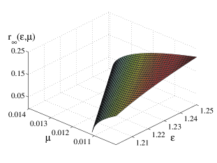
Figure 3: (Color online). Plot of $r_{\infty}=\sqrt{\lambda/|\beta|}>0$ for $\mu>\mu_{c}$ as function of $\epsilon$ and $\mu$ according to (4) and (7). We notice that $r_{\infty}$ increases when $\epsilon$ is raised and $\mu$ is lowered.

We notice that the linear terms contribute to the frequency $\omega$ through $\omega_{0}$ (natural frequency), while nonlinearity gives rise to an additional contribution ($-\lambda\alpha/|\beta|$). According to (3.2), the limit cycle $\bar{\bm{\sigma}}(t)$ is approached exponentially fast in time, $r(t)-r_{\infty}\propto e^{-2\lambda t}$.

As they result from a third-order expansion, the predictions of (3.2) are accurate for mutation rates close to the critical value $\mu_{c}$ (with $\epsilon$ fixed), i.e. for “small” positive values of $\lambda$ and $r_{\infty}$ as illustrated in Fig. 4.

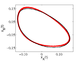
Figure 4: (Color online). With $\bar{x}_{A}(t)=\bar{a}(t)-\frac{1}{3}$ and $\bar{x}_{B}(t)=\bar{b}(t)-\frac{1}{3}$, comparison of the limit cycle obtained from the numerical solution of (3) (red/thick, here $550\leq t\leq 1000$) with the predictions of (3.2) [black/thin]. The parameters and initial conditions are $\epsilon=1.2,~{}\mu=0.01,x_{A}(0)=0.025,x_{B}(0)=0.040$, here $\lambda=1/300$.

To conclude this section, we also consider the case where $\lambda<0$ and notice that Eqs. (3.2) thus yield $r(t)\stackrel{{\scriptstyle t\to\infty}}{{\longrightarrow}}e^{-|\lambda|t}$. This implies that ${\bm{s}}^{*}$ is approached in an oscillatory manner with an exponentially damped amplitude, namely $x_{A}(t)\propto e^{-|\lambda|t}\;\left(\cos{(\omega_{0}t)}-\sin{(\omega_{0}t)}/\sqrt{3}\right)$ and $x_{B}(t)\propto e^{-|\lambda|t}\;\sin{(\omega_{0}t)}$. Furthermore, in the marginal case $\lambda=0$ (with $\mu>0$), ${\bm{s}}^{*}$ is still stable but approached in a slow oscillatory manner. In fact, it follows from (3.2) that in this case $r(t)\sim t^{-1/2}$, which implies that the oscillations are damped algebraically as $t^{-1/2}$. Indeed, for $\lambda=0$ one finds $x_{A}(t)\stackrel{{\scriptstyle t\to\infty}}{{\longrightarrow}}\left[\cos{(\omega_{0}t)}-\frac{1}{\sqrt{3}}\sin{(\omega_{0}t)}\right]/(6\sqrt{\mu t})$ and $x_{B}(t)\stackrel{{\scriptstyle t\to\infty}}{{\longrightarrow}}\sin{(\omega_{0}t)}/(3\sqrt{3\mu t})$.

4 The Stochastic Nonlinear Dynamics

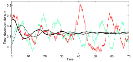
Figure 5: (Color online). Erratic oscillations and stochastic dynamics of the model RPSM in the region (a) of the parameter space, with $\epsilon=0.5,\mu=0.01$ and $N=300$ (initially $N_{A}=135$ and $N_{B}=66$). In single realizations, the time-dependent densities (relative abundances) of species $A$ (thin, red/dark grey) and $B$ (thin, cyan/light grey) are characterized by persistent stochastic oscillations resulting from a resonance amplification occurring at frequency $\Omega^{*}\simeq\omega_{0}\simeq 0.43$ (see text). When they are sample-averaged (here over $200$ replicates), the mean densities (solid and dashed thick curves for species $A$ and $B$, respectively) display damped oscillations approaching the value $1/3$, in agreement with (3).

We so far have focused on the deterministic description of the model in the mean-field limit. However, as virtually all real systems are of finite size, $N<\infty$, and made of discrete entities, they are influenced by stochastic fluctuations. Here, adopting an individual-based approach, we discuss how demographic noise alters the deterministic properties of the model RPSM.

Before mathematically studying the model RPSM in the presence of demographic noise, it is worth gaining some insight into its stochastic dynamics. As explained below, the latter has been implemented by a birth-death process simulated according to the Gillespie algorithm (Gillespie (1976, 1977)). Some characteristic results are reported in Figs. 5-7. The behavior corresponding to the regime (a) of the parameter space (see Fig. 2) is illustrated in Fig. 5, where demographic noise causes erratic oscillations forming “(phase-forgetting) quasi-cycles” (Nisbet and Gurney (1982)) in the phase portrait (see also Fig. 7, cyan/light grey trajectory). When the population size $N$ is large and sample-averaged over many replicates, the amplitude of the stochastic oscillations decreases and the predictions of the rate equations are approached (thick curves in Fig. 5), but fully recovered only in the mean-field limit $N\to\infty$. The stochastic dynamics in the region (b) of the parameter space, where ${\bm{s}}^{*}$ is unstable, is illustrated in Fig. 6 and is characterized by persistent oscillations with erratic, but non-vanishing, amplitude and phase. As a result, instead of a perfectly closed orbit the trajectories in the phase portrait form a perturbed limit cycle, also called “phase-remembering quasi-cycle” (Nisbet and Gurney (1982)), as shown in Fig. 7 (red/dark grey trajectory). Figs. 5 and 6 show that demographic noise affects considerably each single realization in the region (a) of the parameter space, where the predictions of the REs are replaced by oscillations of non-vanishing amplitude, while it perturbs the cyclic behavior in region (b). Below, we show that the “quasi-cycles” arising in region (a) of Fig. 2 at low mutation rate result from a resonance amplification mechanism (McKane and Newman (2005)). We will also see how noise affects the system’s attractors that can be regarded as minima of an effective potential well from which it takes an enormous amount of time to escape (Gardiner (2002); Kubo et al. (1973); Dykman et al. (1994); Volovik et al. (2009)).

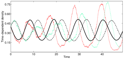
Figure 6: (Color online). Stochastic dynamics of the model RPSM in the region (b) of the parameter space with $\epsilon=1.25,\mu=0.008$ and $N=600$ (initially $N_{A}=N_{B}=240$). We notice that the averaged (over $250$ replicates) time-dependent densities of species $A$ (thick, solid) and $B$ (thick, dashed) are characterized by oscillations of non-vanishing amplitude. The erratic trajectories in red/dark grey and cyan/light grey are single realizations (no sample averaging) of the density of species $A$ and $B$, respectively.

To describe the stochastic nonlinear dynamics of the system, we adopt an individual-based approach and consider an urn model (Feller (1968)) comprising a total of $N=N_{A}+N_{B}+N_{C}$ individuals, $N_{A}$ are of species $A$, $N_{B}$ of species $B$, and $N_{C}$ of species $C$. Up to fluctuation of order ${\cal O}(N^{-1/2})$  (see below), the densities of species $A$, $B$ and $C$ are respectively $a=N_{A}/N$, $b=N_{B}/N$ and $c=N_{C}/N=1-a-b$. The stochastic dynamics is here implemented according to the frequency-dependent Moran process (fMP) (Nowak et al. (2004); Nowak (2006)) (see also (Moran (1958); Blythe and McKane (2007))). The latter is a Markovian process in which, at each time step, two individuals – say one of species $A$ and another of species $B$ – are randomly selected and then reproduce according to their fitness, here proportional to the individual’s average payoff. Once the density-dependent average payoffs are determined, one of the individual, say $A$, reproduces with a rate $T^{B\to A}$ and the offspring replaces a randomly chosen individual of the other species ($B$ in this example). The fMP therefore conserves the total size $N$ of the population and can be regarded as a random-walk with hopping rates depending on each species average payoff (fitness). While there are various ways of implementing the dynamics of the fMP, we here consider that in the absence of mutations and large (yet finite) population size the transition $T^{B\to A}$ from $B$ to $A$, say, is given by $[1+\left(\pi_{A}-\bar{\pi}\right)]\,ab$. This expression comprises a contribution proportional to the average payoff differences $(\pi_{A}-\bar{\pi})$, that accounts for selection, supplemented by a constant (set to $1$) accounting for the background random noise (Nowak et al. (2004); Nowak (2006)). The multiplying factor $ab$ encodes the probability (when $N\gg 1$) that two individuals of species $A$ and $B$ interact. The effect of mutations is thus taken into account by adding a linear term, which finally leads to the following transition rate: $T^{B\to A}({\bm{s}})=\left(1+\{\pi_{A}-\bar{\pi}\}\right)\,ab+\mu b$. More generally, we consider the following transition rates:

$$T^{i\to j}({\bm{s}}) = \left(1+\{\pi_{j}-\bar{\pi}\}\right)\,s_{i}s_{j}+\mu s_{i},$$ (10)

with $i\neq j\in(A,B,C)$ and $\pi_{A}=c-\epsilon b$, $\pi_{B}=a-\epsilon c$, $\pi_{C}=b-\epsilon a$ and $\bar{\pi}=(1-\epsilon)(ab+bc+ac)$.

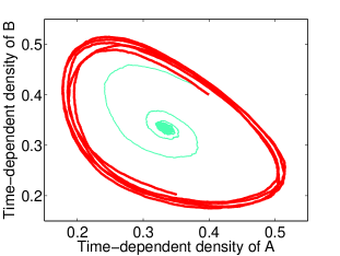
Figure 7: (Color online). Phase portrait of the model RPSM in the presence of stochastic fluctuations for $\epsilon=1.25,N=600$, with $\mu=0.008$ (thick, red/dark grey) and $\mu=0.05$ (thin, cyan/light grey), initially $N_{A}=N_{B}=240$. The trajectories have been obtained from a sample-average over $250$ replicates. When $\mu=0.008$, the interior fixed point ${\bm{s}}^{*}$ is unstable and each trajectory in the phase portrait forms a “phase-remembering quasi-cycle”of erratic non-vanishing amplitude and phase orbiting around $\bar{\bm{\sigma}}$. When $\mu=0.05$, the flow spirals towards the stable interior fixed point ${\bm{s}}^{*}$ and erratically wanders in its vicinity forming a “phase-forgetting quasi-cycle” (see text).

The stochastic description of the system is encoded in the probability $P(N_{A},N_{B};t)$ of having $N_{A}$ and $N_{B}$ individuals of species $A$ and $B$, respectively, at time $t$. The quantity $P(N_{A},N_{B};t)$ obeys the master equation associated with the above fMP (see, e.g., (Gardiner (2002); Ewens (2004))) and specified by the transition rates (10). The Markovian process defined by the transition rates (10) has been simulated using the Gillespie algorithm (Gillespie (1976, 1977)) which was initially introduced to simulate chemical systems through their “microscopic reactions”. In the vicinity of ${\bm{s}}^{*}$ and for large (yet finite) population size, the master equation of the above fMP can be aptly described within a generalized diffusion approximation for the probability density $P({\bm{x}},t)$, where ${\bm{x}}=(x_{A},x_{B})$ and $x_{j}\equiv\frac{N_{j}}{N}-\frac{1}{3},\;j\in(A,B)$ are considered continuous variables (about which we expect fluctuations of order $N^{-1/2}$, see below). The temporal development of $P(x_{A},x_{B};t)$ is thus described by a forward Kolmogorov equation (FKE), or Fokker-Planck equation, resulting from a size-expansion of the master equation (see, e.g., (Gardiner (2002); Ewens (2004); Nisbet and Gurney (1982); Traulsen et al. (2005))). Performing a (linear) van Kampen expansion (van Kampen (1992)) about the fixed point ${\bm{s}}^{*}$ in the continuum limit (assuming that $N$ is large but finite), the standard procedure (see, e.g., (Gardiner (2002); Risken (1989); Reichenbach et al. (2006))) leads to the following FKE:

$$\partial_{t}P({\bm{x}},t)=-\partial_{x_{i}}\left[x_{j}{\cal A}_{ij}({\bm{s}}^{*})P({\bm{x}},t)\right]+\frac{1}{2}{\cal B}_{ij}({\bm{s}}^{*})\partial_{x_{i}}\partial_{x_{j}}P({\bm{x}},t),$$ (11)

where we have adopted the summation convention on repeated indices $i,j\in(A,B)$. In Eq. (11) the drift terms $({\cal A}({\bm{s}}^{*})\,{\bm{x}})_{i}$ are obtained from the Jacobian matrix ${\cal A}$ of the REs (3) at ${\bm{s}}^{*}$ (see Sec. 3.1), while the diffusion matrix ${\cal B}$ is defined by (see, e.g., (Claussen and Traulsen (2008)))

$${\cal B}_{AA}({\bm{s}}^{*}) = T^{B\to A}({\bm{s}}^{*})+T^{A\to B}({\bm{s}}^{*})+T^{C\to A}({\bm{s}}^{*})+T^{A\to C}({\bm{s}}^{*})=\frac{4(1+3\mu)}{9N}$$

$${\cal B}_{BB}({\bm{s}}^{*}) = T^{A\to B}({\bm{s}}^{*})+T^{B\to A}({\bm{s}}^{*})+T^{C\to B}({\bm{s}}^{*})+T^{B\to C}({\bm{s}}^{*})=\frac{4(1+3\mu)}{9N}$$ (12)

$${\cal B}_{AB}({\bm{s}}^{*}) = {\cal B}_{BA}({\bm{s}}^{*})=-\left\{T^{A\to B}({\bm{s}}^{*})+T^{B\to A}({\bm{s}}^{*})\right\}=-\frac{2(1+3\mu)}{9N}.$$

As well known, the FKE (11) is equivalent to the following set of linear stochastic (Langevin) differential equations with Gaussian white noise vector ${\bm{\eta}}=(\eta_{A},\eta_{B})$ (Gardiner (2002); Risken (1989)):

$$\dot{x}_{A} = {\cal A}_{AA}({\bm{s}}^{*})\;x_{A}+{\cal A}_{AB}({\bm{s}}^{*})\;x_{B}+\eta_{A}$$

$$\dot{x}_{B} = {\cal A}_{BA}({\bm{s}}^{*})\;x_{A}+{\cal A}_{BB}({\bm{s}}^{*})\;x_{B}+\eta_{B},$$ (13)

with $\langle\eta_{i}\rangle=0$ and covariance matrix $\langle\eta_{i}(t)\eta_{j}(t^{\prime})\rangle={\cal B}_{ij}({\bm{s}}^{*})\,\delta(t-t^{\prime})$, where $i,j\in(A,B)$ and $\langle...\rangle$ denotes the ensemble average over a large number of replicates. As anticipated, it follows from (4,4) that the noise strength is $\propto N^{-1/2}$ and yields fluctuations of order ${\cal O}(N^{-1/2})$ around the deterministic values of $x_{A}$ and $x_{B}$.

Below, the discussion of stochastic effects on the evolutionary dynamics of the model are centred on two aspects: (i) we show how demographic noise leads to the emergence of quasi-cycles; (ii) and we compute the average time for a system with the same initial density of each species to “escape” from the interior rest point and reach a given cycle.

4.1 Quasi-cycles and noise-induced resonance amplification

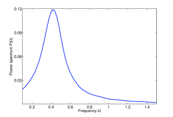
Figure 8: (Color online). Power spectrum $P(\Omega)=\langle|{\widetilde{\bm{x}}}(\Omega)|^{2}\rangle$ of the model RPSM with $\epsilon=0.5,\mu=0.01$ and $N=300$ obtained from numerical simulations and by sample averaging over $200$ realizations. We notice an isolated peak at characteristic frequency $\Omega^{*}\simeq 0.43$, in full agreement with the analytical prediction (15).

In this section, we are especially interested in the stochastic dynamics in region (a) of the phase parameter, where $\lambda<0$ and ${\bm{s}}^{*}$ is a stable fixed point. Here, we investigate one of the most intriguing effects of intrinsic noise, which yields persistent erratic oscillations around ${\bm{s}}^{*}$ (see Fig. 5) and therefore considerably alters the predictions of the REs (3). In fact, while one could naively expect only small corrections (of order $N^{-1/2}$, see Eqs. (4,4)) to the deterministic predictions, it has been suggested that demographic noise can be sufficient to perturb the stationary state predicted by the mean-field analysis and to produce persistent erratic oscillations (see e.g. (Bartlett (1957, 1960))). This is indeed illustrated by the numerical simulations reported in Fig. 5. It has recently been shown that such a behavior, often referred to as quasi-cyclic (Nisbet and Gurney (1982)), results from a resonant amplification of demographic (intrinsic) fluctuations (McKane and Newman (2005)). To analytically demonstrate this phenomenon, we shall compute the power-spectrum $P(\Omega)$ of the system. The power-spectrum is one of the most useful tools to look for oscillations in noisy data and is related to the auto-correlation functions of (stationary) systems (Nisbet and Gurney (1982); Gardiner (2002)). Introducing ${\widetilde{\bm{x}}}(\Omega)\equiv\frac{1}{2\pi}\int_{-\infty}^{\infty}dt\;e^{-i\Omega t}\,{\bm{x}}(t)$, the Fourier transform of ${\bm{x}}(t)$, the power spectrum is given by the following ensemble average: $P(\Omega)=\langle|{\widetilde{\bm{x}}}(\Omega)|^{2}\rangle=2\langle|{\widetilde{x}_{A}}(\Omega)|^{2}\rangle=2\langle|{\widetilde{x}_{B}}(\Omega)|^{2}\rangle$. Taking the Fourier transform of Eqs. (4) and then averaging the square modulus of ${\widetilde{\bm{x}}}(\Omega)$ one finds:

$$P(\Omega) = \frac{8(1+3\mu)}{9N}\quad\frac{\Omega_{0}^{2}+\Omega^{2}}{\left(\Omega^{2}-\Omega_{0}^{2}\right)^{2}+\left(2\lambda\Omega\right)^{2}},$$

$$\text{with}\quad 9\Omega_{0}^{2} \equiv 1+2\sqrt{3}\epsilon\omega_{0}+9\mu(9\mu+1-\epsilon).$$ (14)

For low mutation rate $\mu$ (i.e. when $\mu/\epsilon\ll 1$), $\Omega_{0}^{2}>2\lambda^{2}$ and the power spectrum $P(\Omega)$ has a single peak (for $\Omega>0$) at the characteristic frequency

$$\Omega^{*} = \Omega_{0}\left(2\sqrt{1-\left(\frac{\lambda}{\Omega_{0}}\right)^{2}}-1\right)^{1/2},$$ (15)

as illustrated in Fig. 8. When the mutation rate $\mu$ is low, the value of $\Omega^{*}$ is very close to (yet different from) $\omega_{0}$ and $\Omega_{0}$ (4, 4.1) . When $(\lambda/\Omega_{0})^{2}\ll 1$, the above expression simplifies to give $\Omega^{*}=\Omega_{0}(1+O(\lambda^{2}/\Omega_{0}^{2}))$. It is also worth noticing that at the onset of the Hopf bifurcation, i.e. when $\lambda=0$ (with $\mu>0$), the denominator of $P(\Omega)$ vanishes for $\Omega=\Omega_{0}$ and in this case the peak in the power spectrum is replaced by a pole at $\Omega=\Omega^{*}=\Omega_{0}$.

While on general grounds (law of large numbers (Feller (1968))) one expects oscillations of the order $N^{-1/2}$, the presence of a peak in the power spectrum corresponds to a noise-induced amplification due to a resonance effect. In fact, there is a resonant behavior when there exists a particular frequency for which the denominator of the power spectrum $P(\Omega)$ is small. Here, the denominator of the power spectrum takes its minimal value at

$$\Omega_{\rm res}=\sqrt{\Omega_{0}^{2}-2\lambda^{2}},$$ (16)

which simplifies when $(\lambda/\Omega_{0})^{2}\ll 1$ and also gives $\Omega_{\rm res}=\Omega_{0}(1+O(\lambda^{2}/\Omega_{0}^{2}))$. In such a regime, where $\Omega^{*}\simeq\Omega_{\rm res}\simeq\Omega_{0}$, there is a very suggestive explanation of the noise-induced resonant amplification by comparison with a simple mechanical system (McKane and Newman (2005)). Indeed, one can consider a linear damped harmonic oscillator of natural frequency $\Omega_{0}$, with damping constant $\zeta$, driven by a force oscillating with frequency $\Omega$. One can thus show that such a mechanical system oscillates at frequency $\Omega$, with amplitude ${\rm A_{amp}}(\Omega)\propto\left[(\Omega^{2}-\Omega_{0}^{2})+(\zeta\Omega)^{2}\right]^{-1}$ and yields a resonant frequency $\Omega_{\rm res}=\sqrt{\Omega_{0}^{2}-\frac{\zeta^{2}}{2}}$. Thus, the quantity $2\lambda$ can be interpreted as the damping constant $\zeta$ of the mechanical system. Therefore, provided that $2\lambda$ is much smaller than $\Omega_{0}$ (i.e. $\lambda^{2}/\Omega_{0}^{2}\ll 1$), the model’s dynamics is essentially the same as for a linear damped harmonic oscillator with a resonant frequency $\Omega_{\rm res}=\Omega_{0}$. Yet, while the driving frequency has to be tuned to achieve resonance in the mechanical system, this is not the case for the noisy system that we are considering. In fact, as the model RPSM is driven by internal (Gaussian) white noise (demographic stochasticity) which covers all frequencies, the resonant frequency of the system will be excited without need of any external tuning.

Other fruitful quantities to measure repetitiveness and (quasi-)periodicity in a fluctuating population are the autocorrelation functions $\langle x_{A}(\tau+t)x_{A}(\tau)\rangle=\langle x_{B}(t+\tau)x_{B}(t)\rangle$ and $\langle x_{A}(\tau+t)x_{B}(\tau)\rangle=-\langle x_{B}(\tau+t)x_{A}(\tau)\rangle$. The latter are related to the the power spectrum by the Wiener-Khinchin theorem and can be computed by the Fourier transform of $P(\Omega)$ (Gardiner (2002)), which yields (for $t\geq\tau\gg 1$)

$$\langle x_{A}(\tau+t)x_{A}(\tau)\rangle = \frac{4(1+3\mu)}{3N}\;\frac{e^{-|\lambda|t}}{|\lambda|}\,\cos{(\omega_{0}t)},$$

$$\langle x_{A}(\tau+t)x_{B}(\tau)\rangle = \frac{2(1+3\mu)}{3N}\;\frac{e^{-|\lambda|t}}{|\lambda|}\left\{\sqrt{3}\sin{(\omega_{0}t)}-\cos{(\omega_{0}t)}\right\}.$$ (17)

Following Ref. (Nisbet and Gurney (1982)), fluctuations are non-cyclic if the auto-correlation functions decay monotonically to zero, whereas they lead to quasi-cycles if the auto-correlations oscillate. In the latter case, quasi-cycles are “phase-forgetting” if the oscillations of the auto-correlation functions are damped, as in Eqs. (4.1), and “phase-remembering” when their amplitude do not vanish. Following this classification, it is clear from (4.1) and Figs. 5 and 6 that the quasi-cycles in the region (a) of the parameter space are “phase-forgetting”, while those in the region (b) are “phase-remembering”.

An analysis similar to that of this section can be carried out in the region (b) of the phase parameter by performing a van Kampen expansion around the limit cycle $\bar{\bm{\sigma}}(t)$. This leads to deal with a stochastic version of non-autonomous linear differential equations (see, e.g., (Boland et al. (2008))).

4.2 Average escape time

Another intriguing effect of demographic noise is related to the pivotal concepts of attractor and stability. As discussed in the previous sections there are two different types of stable attractors in the model RPSM: ${\bm{s}}^{*}=(1/3,1/3,1/3)$ is the only attractor of the system when $\lambda\leq 0$, whereas all trajectories in the phase portrait approach the limit cycle $\bar{{\bm{\sigma}}}=(\bar{a}(t),\bar{b}(t))$ when $\lambda>0$. This scenario predicting drastically different fate depending on whether $\lambda\leq 0$ or $\lambda>0$ has to be revised when fluctuations are accounted. In this case, within a probabilistic setting, attractors can be regarded as minima of a potential well from which it is always possible to escape after some characteristic time (which can be enormously long, see, e.g., (Gardiner (2002); Risken (1989); Kubo et al. (1973); Dykman et al. (1994); Volovik et al. (2009))). Stochasticity affects the concept of stability even if the system is initially at the fixed point ${\bm{s}}^{*}$. In fact, due to demographic fluctuations, the species densities deviate from ${\bm{s}}^{*}$ and yield quasi-cycles resulting in persistent erratic oscillations of non-vanishing amplitude. It is therefore biologically relevant to assess the robustness of the population composition and understand how noise affects the co-evolution of sub-populations that initially coexist with the same density. Here, to further assess the influence of intrinsic fluctuations when $N$ is large yet finite, we are interested in the average time to escape from ${\bm{s}}^{*}$ and reach a specified separating distance from it. In other words, we compute the average time $T_{{\rm esc}}(R)$ for a trajectory starting at ${\bm{s}}^{*}$ to reach a cycle ${\cal C}(R)$ on which oscillations around ${\bm{s}}^{*}$ are of amplitude $2R/\sqrt{3}$ (see below). Below, we discuss our results, that are summarized in Fig. 9, and also present an analytical approach – based on the diffusion theory and van Kampen expansion – to compute ${\cal T}_{{\rm esc}}(R)$, that is an accurate approximation of $T_{{\rm esc}}(R)$ around ${\bm{s}}^{*}$.

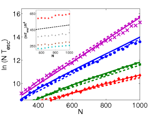
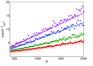
Figure 9: (Color online). Average escape time $T_{\rm esc}(R)$ to reach the cycles ${\cal C}(R)$ starting from ${\bm{s}^{*}}$, for $R=0.10~{}(\Diamond),0.12~{}(\Box),0.15~{}(\bullet),0.17~{}(\times)$ and large population size $N$. Left: Plot of $\ln{(NT_{\rm esc}(R))}$ versus $N$ in the case $\lambda<0$, with $\epsilon=0.5$ and $\mu=0.01$, and sample-average over $100$ replicates. We find a linear dependence that yields $T_{\rm esc}(R)\propto e^{C_{1}(R)~{}N}/N$. Numerical results (filled symbols) are also compared to the predictions of Eqs. (21) (solid) and (22) (dashed), yielding $C_{1}(R)\propto R^{2}$. Right: Plot of ${\rm exp}{(2\lambda T_{\rm esc}(R))}$ versus $N$ in the case $\lambda>0$, with $\epsilon=1.5$ and $\mu=0.01$ and sample-average over $400$ replicates. The observed linear dependence yields $T_{\rm esc}(R)\propto\ln{(C_{2}(R)~{}N)}/(2\lambda)$. Numerical results (filled symbols) are also compared to the predictions of Eqs. (21) (solid) and (23) (dashed lines, almost indistinguishable from the solid lines), yielding $C_{2}(R)\propto R^{2}$. Inset: Marginal case $\lambda=0$ with parameters $\epsilon=1.18$ and $\mu=0.01$, and sample-average over $100$ replicates. Plot of $R^{-4}\ln{(T_{\rm esc}(R))}$ versus $N$ for values of $R=0.30~{}(\star),0.35~{}(\triangle),0.40~{}(\nabla),0.45~{}(+)$. For large population size, the (approximate) linear dependence $R^{-4}\ln{(T_{\rm esc}(R))}\propto 0.23N$ (dashed line as a guide for the eyes) yields $T_{\rm esc}(R)\sim e^{0.23R^{4}N}$ (see text).

Using the Gillespie algorithm, we have computed numerically the average escape time $T_{{\rm esc}}(R)$ necessary to reach a cycle ${\cal C}(R)$ starting from the interior fixed point $a^{*}=b^{*}=c^{*}=1/3$ (same initial density of each species). To exploit the symmetry of the model (see Sec. 3.2), we work with the variables ${\bm{y}}=(y_{A},y_{B})={\cal S}{\bm{x}}$ and consider cycles ${\cal C}(R)$ of parametric equation $y_{A}=R\cos{\phi},\;y_{B}=R\sin{\phi}$. In the original ${\bm{x}}-$variables, the equation of ${\cal C}(R)$ is $x_{A}=R\left(\cos{\phi}-\sin{\phi}/\sqrt{3}\right),\,x_{B}=(2R/\sqrt{3})\sin{\phi}$ and the amplitude of the oscillations is $2R/\sqrt{3}$. In our numerical computations, we have considered systems of population size $N$, with $N=300-4000$, and values of $R$ ranging from $0.10$ to $0.45$. Each simulation has been sample-averaged over $100$ to $400$ replicates. As we are mainly interested in the linear regime around ${\bm{s}}^{*}$, where analytical calculations are amenable (see below), particular attention has been dedicated to values of $R\approx 0.10-0.20$ (i.e. amplitude $\approx 0.11-0.23$). Typical results are reported in Fig. 9, where one essentially distinguishes two cases. If $\lambda<0$, ${\bm{s}}^{*}$ is stable and $\ln{(NT_{\rm esc}(R))}$ grows linearly with $N$ (for large $N$) with a slope depending on $R$, as illustrated in Fig. 9 (left), which yields $T_{\rm esc}(R)\propto e^{C_{1}(R)N}/N$. On the other hand, when ${\bm{s}}^{*}$ is unstable ($\lambda>0$) and $N$ is large, we find that ${\rm exp}(2\lambda T_{\rm esc}(R))$ varies linearly with $N$ (slope depending on $R$), as shown in Fig. 9 (right). This leads to $T_{\rm esc}(R)\propto\ln{(C_{2}(R)~{}N)}/(2\lambda)$. In the above asymptotic expressions, $C_{1}(R)$ and $C_{2}(R)$ are monotonic functions of $R$ and comparison with analytical calculations around ${\bm{s}}^{*}$ suggests that $C_{1}\sim C_{2}\propto R^{2}$ (see below). For the marginal case $\lambda=0$ and large $N$, numerical results are reported in the inset of Fig. 9 (left) and we find that $(\ln{T_{\rm esc}(R))/R^{4}}$ (approximately) exhibits a linear dependence on $N$ (with constant slope). In the case $\lambda=0$, one thus finds $T_{\rm esc}(R)\sim e^{C_{3}R^{4}N}$, where $C_{3}$ is a constant.

In the realm of the diffusion theory and van Kampen expansion, the calculation of the (approximate) average escape time ${\cal T}_{{\rm esc}}({\bm{x}})$ can be regarded as a first-passage problem to an absorbing cycle ${\cal C}(R)$ starting from a system initially at ${\bm{s}}^{*}$ (Gardiner (2002); Redner (2001)). To obtain an equation for ${\cal T}_{{\rm esc}}$ it is useful to consider the so-called backward Kolmogorov equation (BKE), which is the adjoint of Eq. (11) and reads (see, e.g., (Gardiner (2002); Risken (1989); Redner (2001))):

$$-\partial_{t}P_{b}({\bm{x}},t) = {\cal L}_{b}P_{b}({\bm{x}},t),$$

$$\text{with}\quad{\cal L}_{b}({\bm{x}}) = {\cal A}_{ij}({\bm{s}}^{*})x_{j}\;\partial_{x_{i}}+\frac{1}{2}\,{\cal B}_{ij}({\bm{s}}^{*})\partial_{x_{i}}\partial_{x_{j}}.$$ (18)

As in Section 3.2, to reveal the polar properties of the system in the vicinity of ${\bm{s}}^{*}$, it is natural to perform the linear transformation ${\bm{x}}\to{\bm{y}}={\cal S}{\bm{x}}$ and work in the ${\bm{y}}-$variables. Under this transformation, one has $P_{b}({\bm{x}},t)\to{\widetilde{P}}_{b}({\bm{y}},t)$, ${\cal A}({\bm{s}}^{*})\to{\cal S}{\cal A}({\bm{s}}^{*}){\cal S}^{-1}=\begin{pmatrix}\lambda&-\omega_{0}\\ \omega_{0}&\lambda\end{pmatrix}$ and ${\cal B}({\bm{s}}^{*})\to{\cal S}{\cal B}({\bm{s}}^{*}){\cal S}^{T}=\frac{1+3\mu}{3N}~{}\begin{pmatrix}1&0\\ 0&1\end{pmatrix}$ (Reichenbach et al. (2006)). Thus, in the ${\bm{y}}-$variables, the differential operator of Eq. (4.2) becomes ${\cal L}_{b}({\bm{x}})\to{\widetilde{\cal L}}_{b}({\bm{y}})=\lambda(y_{A}\partial_{y_{A}}+y_{B}\partial_{y_{B}})+\omega_{0}(y_{B}\partial_{y_{A}}-y_{A}\partial_{y_{B}})-\frac{1+3\mu}{6N}(\partial_{y_{A}}^{2}+\partial_{y_{B}}^{2})$. To exploit the system’s symmetry around ${\bm{s}}^{*}$, we then adopt the polar coordinates $(\rho,\phi)$, with $y_{A}=\rho\cos{\phi}$ and $y_{B}=\rho\sin{\phi}$. The radial BKE thus reads $\partial_{t}{\widetilde{P}}_{b}(\rho,t)={\widetilde{\cal L}}_{b}(\rho){\widetilde{P}}_{b}(\rho,t)$, with

$${\widetilde{\cal L}}_{b}(\rho)=\left[\lambda\rho+\left(\frac{1+3\mu}{6N}\right)\frac{1}{\rho}\right]\partial_{\rho}+\left(\frac{1+3\mu}{6N}\right)\partial_{\rho}^{2}$$ (19)

To derive the above radial operator, we have assumed that the initial radial symmetry of the probability distribution (initially the system is at ${\bm{s}}^{*}$, without any angular dependence) is approximately preserved by the dynamics. The above approach is certainly valid at linear order around ${\bm{s}}^{*}$ and is consistent with the van Kampen linear expansion that has led to (11) and (4.2). With (19), the equation for the average escape time ${\cal T}_{{\rm esc}}(\rho)$ at a distance $\rho$ from ${\bm{s}}^{*}$ is given by (Gardiner (2002); Risken (1989))

$$-1={\widetilde{\cal L}}_{b}(\rho)~{}{\cal T}_{{\rm esc}}(\rho).$$ (20)

In the framework of diffusion and van Kampen approximations, we now analytically compute the mean escape time ${\cal T}_{{\rm esc}}(R)$ for $\rho$ to attain the value $R$ starting from ${\bm{s}}^{*}$ (i.e. initially $\rho=0$), which corresponds to the mean time necessary to reach the cycle ${\cal C}(R)$. Our analytical treatment is valid in the linear regime around ${\bm{s}}^{*}$, where $\phi\simeq\omega_{0}$, and the amplitude of the oscillations on ${\cal C}(R)$ is $2R/\sqrt{3}$. In our theoretical setting, the average escape time ${\cal T}_{{\rm esc}}(R)$ is obtained by solving Eq. (20) subject to a reflecting and an absorbing boundary conditions at $\rho=0$ and $\rho=R$, respectively (Gardiner (2002)). When $\lambda\neq 0$, the solution to this problem can be expressed in terms of the function $\Psi(z)=z\,{\rm exp}\left(\frac{3N\lambda}{1+3\mu}~{}z^{2}\right)$:

$${\cal T}_{{\rm esc}}(R) = \left(\frac{6N}{1+3\mu}\right)~{}\int_{0}^{R}\frac{dy}{\Psi(y)}~{}\int_{0}^{y}~{}dz\Psi(z)=\frac{1}{2\lambda}\int_{0}^{-\frac{3NR^{2}\lambda}{1+3\mu}}\frac{du}{u}~{}\left(1-e^{u}\right).$$ (21)

The solid curves in Fig. 9 show the comparison between the prediction (21) and numerical results. We notice that for small values of $R$, e.g., $R=0.10-0.15$, there is an excellent agreement between (21) and the results of numerical simulations (both in the cases $\lambda<0$ and $\lambda>0$). For larger values of $R$ (e.g. for $R\geq 0.17$), nonlinearities and non-vanishing angular dependence cause some systematic deviations from the results of numerical computations (discrepancies of $\approx 5\%-10\%$ in the results of Fig. 9 for $R=0.17$), but (21) still provides the correct (qualitative) behavior and a reasonable approximation of $T_{{\rm esc}}(R)$. In the asymptotic limit of large population size $N$, two distinct behaviors can be obtained from Eq. (21):

• When $\lambda<0$, ${\bm{s}}^{*}$ is stable and the main contribution to (21) is given by ${\cal T}_{{\rm esc}}(R)\simeq\frac{1}{2|\lambda|}~{}{\rm Ei}\left(\frac{3|\lambda|R^{2}N}{1+3\mu}\right)$, where ${\rm Ei}(x)\equiv\int_{-\infty}^{x}dt\,(e^{t}/t)$ is the exponential integral (Abramowitz and Stegun (1965)). From the properties of this function, we infer the following asymptotic behavior (for $|\lambda|NR^{2}\gg 1$):

  $${\cal T}_{{\rm esc}}(R)\simeq\left(\frac{1+3\mu}{6(\lambda R)^{2}N}\right)\,{\rm exp}\left(\frac{3|\lambda|R^{2}N}{1+3\mu}\right)$$ (22)

  This result predicts that the mean escape time increases dramatically with the total number of individuals $N$ and, when $|\lambda|NR^{2}\gg 1$, is proportional to the exponential of the population size. The dashed lines in Fig. 9 (left) illustrate that (22) is a very good approximation of $T_{{\rm esc}}(R)$ in the linear regime around ${\bm{s}}^{*}$, e.g. for $R=0.10-0.15$, when $N\gg 1$ . In particular, we notice that (22) coincides with the aforementioned asymptotic expression of $T_{{\rm esc}}(R)$ with $C_{1}=3|\lambda|R^{2}/(1+3\mu)$. For $R=0.17$, when $N$ is large, nonlinear effects are important and in Fig. 9 the exponent of (22) overestimates that of $T_{{\rm esc}}(R)$ by $\approx 5\%$.

• When $\lambda>0$, demographic fluctuations always cause the departure from ${\bm{s}}^{*}$ (unstable), and all trajectories in the phase portrait are attracted by the limit cycle $\bar{{\bm{\sigma}}}$. In this case, from the properties of the exponential integral (Abramowitz and Stegun (1965)), for $\lambda NR^{2}\gg 1$, the main contribution to (21) is

  $${\cal T}_{{\rm esc}}(R)\simeq\frac{1}{2\lambda}~{}\left[\ln{\left(\frac{3\lambda R^{2}N}{1+3\mu}\right)}+\gamma_{\rm EM}\right],$$ (23)

  where $\gamma_{\rm EM}=0.57721...$ is Euler-Mascheroni’s constant. This result predicts that, when $\lambda NR^{2}\gg 1$, the mean escape time grows logarithmically with the population size $N$, i.e. ${\cal T}_{{\rm esc}}(R)\to(\ln{N})/2\lambda$, and the value of $R$ contributes to subdominant corrections. Here also, the dashed lines in Fig. 9 (right), almost indistinguishable from solid curves, agree very well with the numerically computed $T_{{\rm esc}}(R)$ around ${\bm{s}}^{*}$ (i.e. for $R=0.10-0.15$). We notice that, when $C_{2}=3\lambda R^{2}/(1+3\mu)$, the prediction (23) coincides with the asymptotic expression of $T_{{\rm esc}}(R)$ inferred from Fig. 9 (right).

It is also worth noticing that results (21)-(23) are also valid in the absence of mutations (i.e. when $\mu=0$).

Besides the above cases, a special situation arises when $\lambda=0$, $\mu>0$ and ${\bm{s}}^{*}$ is a center. In fact, in Sec. 3.2, we have seen that in this case ${\bm{s}}^{*}$ is an attractor, but the dynamics in its vicinity is very slow. To account for such a slow dynamics it is not sufficient to consider (11, 4.2) – obtained by linearization about ${\bm{s}}^{*}$ – but nonlinearities have to be accounted. Generalizing the above approach and keeping the cubic terms in the drift contribution (Cremer (2008)), leads to (20) with the following differential operator [instead of (19)]: ${\widetilde{\cal L}}_{b}(\rho)=\left[\{\lambda+\beta\rho^{2}\}\rho+\left(\frac{1+3\mu}{6N}\right)\frac{1}{\rho}\right]\partial_{\rho}+\left(\frac{1+3\mu}{6N}\right)\partial_{\rho}^{2}$. When $\lambda=0$, proceeding as above, one still finds an exponential asymptotic behavior ($\mu R^{4}N\gg 1$): ${\cal T}_{{\rm esc}}(R)\sim N^{-1/2}\,{\rm exp}(27\mu R^{4}N/(1+3\mu))$. This estimate, that is consistent with the numerical results reported in Fig. 9 (left, inset), implies that (at given $R$ and $N$) the mean escape time ${\cal T}_{{\rm esc}}$ around ${\bm{s}}^{*}$ is significantly shorter in the marginal case than in the case $\lambda<0$.

5 Summary and Conclusion

This work has been motivated by the importance of further understanding the mechanisms at the origin of persistent and erratic oscillatory dynamics in population biology, which is frequently observed but whose theoretical origin is often debated. Furthermore, this work concerns the effects of mutations in rock-paper-scissors (RPS) games, which are regarded as paradigmatic models to describe the co-evolutionary dynamics of systems with codominant interactions. It has recently been proposed that codominance can help promote the maintenance of biodiversity, and it is therefore of biological relevance to study generalizations of the RPS model to understand which ingredients favor the long-term coexistence of the sub-populations.

Here, we have investigated the oscillatory dynamics of the generic rock-paper-scissors games with mutations in a well-mixed (homogeneous) population of $N$ individuals. Our study has been carried out in the mean-field limit ($N\to\infty$) and in the presence of demographic noise ($N$ large but finite). In addition to the regions of the parameter space associated with a stable interior fixed point ${\bm{s}}^{*}$ and heteroclinic cycles, the possibility for the individuals to switch from one strategy (species) to another with a small transition rate yields a new oscillatory behavior associated with a limit cycle and resulting from a Hopf bifurcation. In the mean-field limit ($N\to\infty$), we have recast the system’s rate equations in a normal form and studied the main properties of the ensuing limit cycle. When the population size is finite, demographic noise has to be taken into account and the dynamics becomes genuinely stochastic and nonlinear. The latter situation has been described in terms of an individual-based formulation, with the stochastic dynamics implemented according to a Moran process. The influence of intrinsic noise on the dynamics has been analytically assessed within a diffusion theory approximation complemented by numerical simulations (using the Gillespie algorithm). We have shown that demographic noise transforms damped oscillations into (“phase-forgetting”) quasi-cycles and perturbs the amplitude and the phase of limit cycles (that become “phase-remembering” quasi-cycles). As also observed in other systems (e.g., (Bartlett (1957, 1960); Nisbet and Gurney (1982); McKane and Newman (2005); Boland et al. (2008))), the effect of stochasticity is particularly striking in the region of the parameter space where ${\bm{s}}^{*}$ is stable. There, we have found sustained oscillations driven by demographic stochasticity. In fact, while fluctuations are of order $N^{-1/2}$, for small mutation rate, the amplitude of the oscillations is amplified by a resonance amplification caused by internal (white) noise. We have shown that this phenomenon translates into an isolated and well-marked peak in the power-spectrum and have also computed the autocorrelation functions of the system. To further assess the robustness of the co-evolutionary dynamics against noise, we have computed numerically and analytically – using a diffusion approximation and a mapping onto a first-passage problem – the average escape time necessary to reach a cycle on which the oscillations attain a given amplitude. We have therefore shown that such a mean exit time grows either exponentially or logarithmically with the system size, depending on whether the interior fixed point is deterministically stable or unstable, respectively.

In summary, in the presence of mutations the RPS model yields sustained oscillations in every region of the parameter space. The latter are caused by demographic noise and/or result from a Hopf bifurcation. Therefore, mutations in the RPS model ensure that all species co-evolve and oscillate in time without ever going extinct. One can therefore regard mutations as a mechanism favoring the oscillatory dynamics in communities characterized by cyclic co-dominance.

In future research, it would be interesting to consider spatially-extended versions of this model and study how the population will self-organize and which kinds of spatial-temporal patterns would emerge. In particular, as it has recently been shown that mobility can affect co-evolution in RPS models by mediating between mean-field and stochastic dynamics (Reichenbach et al. (2007a, b, 2008b)), it would be relevant to investigate variants of the model RPSM where individuals are allowed to move and interact in space.

References

- Abramowitz and Stegun (1965) Abramowitz, M., Stegun, I. (editors), 1965. Handbook of Mathematical Functions Dover Publications, Inc., New York.
- Anderson and May (1986) Anderson, R. M. et al., 1986. The Invasion, Persistence and Spread of Infectious Diseases within Animal and Plant Communities. Phil. Trans. Roy. Soc. B 314, 533.
- Anderson and May (1991) Anderson, R. M., May, R.M., 1991. Infectious Diseases of Humans. Oxford University Press, Oxford.
- Antal et al (2009) Antal, T., Nowak, M. A., Traulsen, A., 2009. Strategy abundance in 2x2 games for arbitrary mutation rates. J. Theor. Biol. 257, 340.
- Bartlett (1957) Bartlett, M.S., 1957. Measles periodicity and community size. J.R. Stat. Soc. A 120, 48.
- Bartlett (1960) Bartlett, M.S., 1960. The critical community size for measles in the United States. J.R. Stat. Soc. A 123, 37.
- Bastolla et al. (2002) Bastolla U., Lässig M, Manrubia, S. C., Valleriani, A., 2005. Biodiversity in model ecosystems, I: coexistence conditions for competing species. J. Theor. Biol. 235, 521.
- Berr et al. (2009) Berr, M., Reichenbach, T., Schottenloher, M., Frey, E., 2009. Zero-one survival behavior of cyclically competing species. Phys. Rev. Lett. 102, 048102.
- Berryman (2002) Berryman, A. A., 2002. Population Cycles. Oxford University Press, Oxford.
- Blythe and McKane (2007) Blythe, R. A., McKane, A. J., 2007. Stochastic models of evolution in genetics, ecology and linguistics. J. Stat. Mech. P07018.
- Boland et al. (2008) Boland, R. P., Galla, T., McKane, A. J., 2008. How limit cycles and quasi-cycles are related in systems with intrinsic noise. J. Stat. Mech. P09001.
- Claussen and Traulsen (2008) Claussen, J. C., Traulsen, A., 2008. Cyclic Dominance and Biodiversity in Well-Mixed Populations. Phys. Rev. Lett. 100, 058104.
- Cremer (2008) Cremer, J., Reichenbach, T., Frey, E., 2008. Anomalous finite-size effects in the Battle of the Sexes. Eur. Phys. J. B 63, 373.
- Czárán et al. (2002) Czárán, T. L., Hoekstra, R. F., Pagie, L., 2002. Chemical warfare between microbes promotes biodiversity. Proc. Natl. Acad. Sci. U.S.A. 99, 786.
- Dawkins (1976) Dawkins, R., 1976. The Selfish Gene. Oxford University Press, New York.
- Dykman et al. (1994) Dykman, M. I., Mori, E., Ross, J., Hunt, P. M., 1994. Large fluctuations and optimal paths in chemical kinetics. J. Chem. Phys. 100, 5735.
- Durrett and Levin (1994) Durrett, R., Levin, S., 1994. The importance of being discrete (and spatial). Theor. Pop. Biol. 46, 363.
- Durrett and Levin (1997) Durrett, R., Levin, S., 1997. Allelopathy in spatially distributed populations. J. Theor. Biol. 185, 165.
- Elowitz and Leibler (2000) Elowitz, M. B., Leibler, S., 2000. A synthetic oscillatory network of transcriptional regulators. Nature 403, 335.
- Ewens (2004) Ewens, W. J., 2004. Mathematical Population Genetics. Springer Verlag, New York, 2nd ed.
- Feller (1968) Feller, W., 1968. An Introduction to Probability Theory and its Application, vol. 1. Wiley, London, third ed.
- Gardiner (2002) Gardiner, C. W., 2002. Handbook of Stochastic Methods. Springer Verlag, Berlin, 2nd ed.
- Gilg et al. (2001) Gilg, O., Hanski, I., Sittler, B., 2001. Cyclic dynamics in a simple vertebrate predator-prey-community. Science 302, 866.
- Gillespie (1976) Gillespie, D. T., 1976. A general method for numerically simulating the stochastic time evolution of coupled chemical reactions. J. Comp. Phys. 22, 403.
- Gillespie (1977) Gillespie, D. T., 1977. Exact simulations of coupled chemical reactions. J. Phys. Chem. 81, 2340.
- Grimshaw (1994) Grimshaw, R., 1994 Nonlinear Ordinary Differential Equations. CRC Press, Ann Arbor.
- Haken (2002) Haken, H., 2002. Synergetics. Springer Verlag, New York, third ed.
- Hauert et al. (2002) Hauert, C., de Monte, S., Hofbauer, J., Sigmund, K., 2002. Volunteering as Red Queen mechanism for cooperation in public goods games. Science 296, 1129.
- Hofbauer and Sigmund (1998) Hofbauer, J., Sigmund, K., 1998. Evolutionary Games and Population Dynamics. Cambridge University Press, Cambridge.
- Hubbell (2001) Hubbell, S. P., 2001. The Unified Neutral Theory of Biodiversity and Biogeography. Princeton University Press, Princeton.
- Kerr et al. (2002) Kerr, B., Riley, M. A., Feldman, M. W., Bohannan, B. J. M., 2002. Local dispersal promotes biodiversity in a real-life game of rock-paper-scissors. Nature 418, 171.
- Kirkup and Riley (2004) Kirkup, B. C., Riley, M. A., 2004. Antibiotic-mediated antagonism leads to a bacterial game of rock-paper-scissors in vivo. Nature 428, 412.
- Kubo et al. (1973) Kubo, R., Kazuhiro, M., Kitahara, K., 1973. Fluctuation and relaxation of macrovariables. J. Stat. Phys. 9, 51.
- May (1974) May, R. M., 1974. Stability and Complexity in Model Ecosystems. Cambridge University Press, Cambridge.
- May and Leonard (1975) May, R. M., Leonard, W. J., 1975. Nonlinear aspects of competition between species. SIAM J. Appl. Math 29, 243.
- Maynard Smith (1982) Maynard Smith, J., 1982. Evolution and the Theory of Games. Cambridge University Press, Cambridge.
- McKane and Newman (2005) McKane, A.J., Newman, T.J., 2005. Predator-prey cycles from resonant amplification of demographic stochasticity. Phys. Rev. Lett. 94, 218102.
- Michod (2000) Michod, R. E., 2000. Darwinian Dynamics. Princeton University Press, Princeton.
- Mobilia et al. (2007) Mobilia, M., Georgiev, I. T., Täuber, U. C., 2007. Phase Transitions and Spatio-Temporal Fluctuations in Stochastic Lattice Lotka-Volterra Models. J. Stat. Phys. 128, 447.
- Moran (1958) Moran, P. A. P., 1958. Random processes in genetics. Proc. Camb. Phil. Soc. 54, 60.
- Murray (2002) Murray, J. D., 2002. Mathematical Biology. Springer Verlag, New York.
- Neal (2004) Neal, D., 2004. Introduction to Population Biology. Cambridge University Press, Cambridge (USA).
- Nisbet and Gurney (1982) Nisbet, R.M., Gurney, W.S.C., 1982. Modelling fluctuating populations. Wiley, New York.
- Nowak (2006) Nowak, M. A., 2006. Evolutionary Dynamics. Belknap Press, Cambridge (USA).
- Nowak et al. (2004) Nowak, M. A., Sasaki, A., Taylor, C., Fudenberg, D.,2004. Emergence of cooperation and evolutionary stability in finite populations. Nature (London) 428, 646.
- Peltomäki and Alava (2008) Peltomäki, M., Alava, M., 2008. Three- and four-state rock-paper-scissors games with diffusion. Phys. Rev. E 78, 031906.
- Perc et al. (2007) Perc, M., Szolnoki, A., Szabó, G., 2007. Cyclical interactions with alliance-specific heterogeneous invasion rates. Phys. Rev. E 75, 052102.
- Redner (2001) Redner, S., 2001. A Guide to First-Passage Processes. Cambridge University Press, Cambridge.
- Reichenbach et al. (2006) Reichenbach, T., Mobilia, M., Frey, E., 2006. Coexistence versus extinction in the stochastic cyclic Lotka-Volterra model. Phys. Rev. E 74, 051907.
- Reichenbach et al. (2007a) Reichenbach, T., Mobilia, M., Frey, E., 2007a. Mobility promotes and jeopardizes biodiversity in rock-paper-scissors games. Nature 448, 1046–1049.
- Reichenbach et al. (2007b) Reichenbach, T., Mobilia, M., Frey, E., 2007b. Noise and correlations in a spatial population model with cyclic competition. Phys. Rev. Lett. 99, 238105.
- Reichenbach et al. (2008b) Reichenbach, T., Mobilia, M., Frey, E., 2008. Self-Organization of Mobile Populations in Cyclic Competition. J. Theor. Biol. 254, 368.
- Risken (1989) Risken, H., 1989. The Fokker-Planck Equation. Springer Verlag, New York, second ed.
- Sinervo and Lively (1996) Sinervo, B., Lively, C. M., 1996. The rock-scissors-paper game and the evolution of alternative male strategies. Nature 380, 240.
- Strogatz (1994) Strogatz, S. H., 1994. Nonlinear dynamics and chaos. Addison-Wesley Publishing, Reading, MA.
- Szabó and Fath (2007) Szabó, G., Fath, G., 2007. Evolutionary games on graphs. Phys. Rep. 446, 97.
- Szabó and Szolnoki (2002) Szabó, G., Szolnoki, A., 2002. A three-state cyclic voter model extended with Potts energy. Phys. Rev. E 65, 036115.
- Tainaka (1994) Tainaka, K., 1994. Vortices and strings in a model ecosystem. Phys. Rev. E 50, 3401.
- Traulsen et al. (2005) Traulsen, A., Claussen, J. C., Hauert, C., 2005. Coevolutionary dynamics: From finite to infinite populations. Phys. Rev. Lett. 95, 238701.
- Turchin (2003) Turchin, P., 2003. Complex Population Dynamics. Princeton University Press, Princeton.
- van Kampen (1992) van Kampen, N. G., 1992. Stochastic processes in physics and chemistry. North Holland Publishing Company, Amsterdam.
- Volovik et al. (2009) Volovik, D., Mobilia, M., Redner, S., 2009. Dynamics of three-choice voting. EPL 85, 48003.
- Wiggins (1990) Wiggins, S, 1990. Introduction to Applied Nonlinear Dynamical Systems and Chaos. Springer Verlag, New York.
- Zamudio and Sinervo (2000) Zamudio, K. R., Sinervo, B., 2000. Polygyny, mate-guarding, and posthumous fertilization as alternative male mating strategies. Proc. Natl. Acad. Sci. U.S.A. 97, 14427.