Ranking relations using analogies in biological and information networks

Abstract

Analogical reasoning depends fundamentally on the ability to learn and generalize about relations between objects. We develop an approach to relational learning which, given a set of pairs of objects $\mathbf{S}=\{A^{(1)}\dvtx B^{(1)},A^{(2)}\dvtx B^{(2)},\ldots,A^{(N)}\dvtx B^{(N)}\}$, measures how well other pairs $A\dvtx B$ fit in with the set $\mathbf{S}$. Our work addresses the following question: is the relation between objects $A$ and $B$ analogous to those relations found in $\mathbf{S}$? Such questions are particularly relevant in information retrieval, where an investigator might want to search for analogous pairs of objects that match the query set of interest. There are many ways in which objects can be related, making the task of measuring analogies very challenging. Our approach combines a similarity measure on function spaces with Bayesian analysis to produce a ranking. It requires data containing features of the objects of interest and a link matrix specifying which relationships exist; no further attributes of such relationships are necessary. We illustrate the potential of our method on text analysis and information networks. An application on discovering functional interactions between pairs of proteins is discussed in detail, where we show that our approach can work in practice even if a small set of protein pairs is provided.

M1Supported in part by NSF Grant DMS-09-07009, by NIH Grant R01 GM096193, and by the Gatsby Charitable Foundation.

, ,
and

1 Contribution

Many university admission exams, such as the American Scholastic Assessment Test (SAT) and Graduate Record Exam (GRE), have historically included a section on analogical reasoning. A prototypical analogical reasoning question is as follows:

1. [(A)]

2. $\mathtt{doctor\dvtx hospital}$:

3. sports $\mathtt{fan\dvtx stadium}$

4. cow $\mathtt{\dvtx farm}$

5. $\mathtt{professor\dvtx college}$

6. $\mathtt{criminal\dvtx jail}$

7. $\mathtt{food\dvtx grocery}$ store

The examinee has to answer which of the five pairs best matches the relation implicit in $\mathtt{doctor\dvtx hospital}$. Although all candidate pairs have some type of relation, pair $\mathtt{professor\dvtx college}$ seems to best fit the notion of (profession, place of work), or the “works in” relation implicit between doctor and hospital.

This problem is nontrivial because measuring the similarity between objects directly is not an appropriate way of discovering analogies, as extensively discussed in the cognitive science literature. For instance, the analogy between an electron spinning around the nucleus of an atom and a planet orbiting around the Sun is not justified by isolated, nonrelational, comparisons of an electron to a planet, and of an atomic nucleus to the Sun [Gentner (1983)]. Discovering the underlying relationship between the elements of each pair is key in determining analogies.

1.1 Applications

This paper concerns practical problems of data analysis where analogies, implicitly or not, play a role. One of our motivations comes from the bioPIXIE project [Myers et al. (2005)]. bioPIXIE is a tool for exploratory analysis of protein–protein interactions. Proteins have multiple functional roles in the cell, for example, regulating metabolism and regulating cell cycle, among others. A protein often assumes different functional roles while interacting with different proteins. When a molecular biologist experimentally observes an interaction between two proteins, for example, a binding event of $\{P_{i},P_{j}\}$, it might not be clear which function that particular interaction is contributing to. The bioPIXIE system allows a molecular biologist to input a set $\mathbf{S}$ of proteins that are believed to have a particular functional role in common, and generates a list of other proteins that are deduced to play the same role. Evidence for such predictions is provided by a variety of sources, such as the expression levels for the genes that encode the proteins of interest and their cellular localization. Another important source of information bioPIXIE takes advantage of is a matrix of relationships, indicating which proteins interact according to some biological criterion. However, we do not necessarily know which interactions correspond to which functional roles.

The application to protein interaction networks that we develop in Section 5 shares some of the features and motivations of bioPIXIE. However, we aim at providing more detailed information. Our input set $\mathbf{S}$ is a small set of pairs of proteins that are postulated to all play a common role, and we want to rank other pairs $P_{i}\dvtx P_{j}$ according to how similar they are with respect to $\mathbf{S}$. The goal is to automatically return pairs that correspond to analogous interactions.

To use an analogy itself to explain our procedure, recall the SAT example that opened this section. The pair of words ${\mathtt{doctor}\dvtx\mathtt{hospital}}$ presented in the SAT question play the role of a protein–protein interaction and is the smallest possible case of $\mathbf{S}$, that is, a single pair. The five choices A–E in the SAT question correspond to other observed protein–protein interactions we want to match with $\mathbf{S}$, that is, other possible pairs. Since multiple valid answers are possible, we rank them according to a similarity metric. In the application to protein interactions, in Section 5, we perform thousands of queries and we evaluate the goodness of the resulting rankings according to multiple gold standards, widely accepted by molecular and cellular biologists [Ashburner et al. (2000); Kanehisa and Goto (2000); Mewes et al. (2004)].

The general problem of interest in this paper is a practical problem of information retrieval [Manning, Raghavan and Schütze (2008)] for exploratory data analysis: given a query set $\mathbf{S}$ of linked pairs, which other pairs of objects in my relational database are linked in a similar way? We apply this analysis to cases where it is not known how to explicitly describe the different classes of relations, but good models to predict the existence of relationships are available. In Section 4 we consider an application to information retrieval in text documents for illustrative purposes. Given a set of pairs of web pages which are related by some hyperlink, we would like to find other pairs of pages that are linked in a similar way. In information network settings, the proposed method could be useful, for instance, to answer queries for encyclopedia pages relating scientists and their major discoveries, to search for analogous concepts, or to identify the absence of analogous concepts, in Wikipedia. From an evaluation perspective, this application domain provides an example where large scale evaluation is more straightforward than in the biological setting.

In this paper we introduce a method for ranking relations based on the Bayesian similarity criterion underlying Bayesian sets, a method originally proposed by Ghahramani and Heller (2005) and reviewed in Section 2. In contrast to Bayesian sets, however, our method is tailored to drawing analogies between pairs of objects. We also provide supplementary material with a Java implementation of our method, and instructions on how to rebuild the experiments [Silva et al. (2010)].

1.2 Related work

To give an idea of the type of data which our method is useful for analyzing, consider the methods of Turney and Littman (2005) for automatically solving SAT problems. Their analysis is based on a large corpus of documents extracted from the World Wide Web. Relations between two words $W_{i}$ and $W_{j}$ are characterized by their joint co-ocurrence with other relevant words (such as particular prepositions) within a small window of text. This defines a set of features for each $W_{i}\dvtx W_{j}$ relationship, which can then be compared to other pairs of words using some notion of similarity. Unlike in this application, however, there are often no (or very few) explicit features for the relationships of interest. Instead we need a method for defining similarities using features of the objects in each relationship, while at the same time avoiding the mistake of directly comparing objects instead of relations.

One of the earliest approaches for determining analogical similarity was introduced by Rumelhart and Abrahamson (1973). In their paper, one is initially given a set of pairwise distances between objects (say, by the subjective judgement of a group of people). Such distances are used to embed the given objects in a latent space via a multidimensional scaling approach. A related pair $A\dvtx B$ is then represented as a vector connecting $A$ and $B$ in the latent space. Its similarity with respect to another pair $C\dvtx D$ is defined by comparing the direction and magnitude of the corresponding vectors. Our approach is probabilistic instead of geometrical, and operates directly on the object features instead of pairwise distances.

We will focus solely on ranking pairwise relations. The idea can be extended to more complex relations, but we will not pursue this here. Our approach is described in detail in Section 3.

Finally, the probabilistic, geometrical and logical approaches applied to analogical reasoning problems can be seen as a type of relational data analysis [Džeroski and Lavrač (2001); Getoor and Taskar (2007)]. In particular, analogical reasoning is a part of the more general problem of generating latent relationships from relational data. Several approaches for this problem are discussed in Section 6. To the best of our knowledge, however, most analogical reasoning applications are interesting proofs of concept that tackle ambitious problems such as planning [Veloso and Carbonell (1993)], or are motivated as models of cognition [Gentner (1983)]. Our goal is to create an off-the-shelf method for practical exploratory data analysis.

2 A review of probabilistic information retrieval and the Bayesian sets method

The goal of information retrieval is to provide data points (e.g., text documents, images, medical records) that are judged to be relevant to a particular query. Queries can be defined in a variety of ways and, in general, they do not specify exactly which records should be presented. In practice, retrieval methods rank data points according to some measure of similarity with respect to the query [Manning, Raghavan and Schütze (2008)]. Although queries can, in practice, consist of any piece of information, for the purposes of this paper we will assume that queries are sets of objects of the same type we want to retrieve.

Probabilities can be exploited as a measure of similarity. We will briefly review one standard probabilistic framework for information retrieval [Manning, Raghavan and Schütze (2008), Chapter 11]. Let $R$ be a binary random variable representing whether an arbitrary data point $X$ is “relevant” for a given query set $\mathbf{S}$ ($R=1$) or not ($R=0$). Let $P(\cdot|\cdot)$ be a generic probability mass function or density function, with its meaning given by the context. Points are ranked in decreasing order by the following criterion:

$$\frac{P(R=1|X,\mathbf{S})}{P(R=0|X,\mathbf{S})}=\frac{P(R=1|\mathbf{S})}{P(R=0|\mathbf{S})}\frac{P(X|R=1,\mathbf{S})}{P(X|R=0,\mathbf{S})},$$

which is equivalent to ranking points by the expression

$$\log P(X|R=1,\mathbf{S})-\log P(X|R=0,\mathbf{S}).$$ (1)

The challenge is to define what form $P(X|R=r,\mathbf{S})$ should assume. It is not practical to collect labeled data in advance which, for every possible class of queries, will give an estimate for $P(R=1|X,\mathbf{S})$: in general, one cannot anticipate which classes of queries will exist. Instead, a variety of approaches have been developed in the literature in order to define a suitable instantiation of (1). These include a method that builds a classifier on-the-fly using $\mathbf{S}$ as elements of the positive class $R=1$, and a random subset of data points as the negative class $R=0$ [e.g., Turney (2008b)].

The Bayesian sets method of Ghahramani and Heller (2005) is a state-of-the-art probabilistic method for ranking objects, partially inspired by Bayesian psychological models of generalization in human cognition [Tenenbaum and Griffiths (2001)]. In this setup the event “$R=1$” is equated with the event that $X$ and the elements of $\mathbf{S}$ are i.i.d. points generated by the same model. The event “$R=0$” is the event by which $X$ and $\mathbf{S}$ are generated by two independent models: one for $X$ and another for $\mathbf{S}$. The parameters of all models are random variables that have been integrated out, with fixed (and common) hyperparameters. The result is the instantiation of (1) as

$$\log P(X|\mathbf{S})-\log P(X)=\log\frac{P(X,\mathbf{S})}{P(X)P(\mathbf{S})},$$ (2)

the Bayesian sets score function by which we rank points $X$ given a query $\mathbf{S}$. The right-hand side was rearranged to provide a more intuitive graphical model, shown in Figure 1. From this graphical model interpretation we can see that the score function is a Bayes factor comparing two models [Kass and Raftery (1995)].

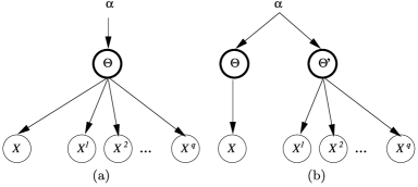
Figure 1: In order to score how well an arbitrary element $X$ fits in with query set $\mathbf{S}=\{X^{1},X^{2},\ldots,X^{q}\}$, the Bayesian sets methodology compares the marginal likelihood of the model in (a), $P(X,\mathbf{S})$, against the model in (b), $P(X)P(\mathbf{S})$. In (a), the random parameter vector $\Theta$ is given a prior defined by the (fixed) hyperparameter $\alpha$. The same (latent) parameter vector is shared by the query set and the new point. In (b), the parameter vector $\Theta$ that generates $X$ is different from the one that generates the query set.

In the next section we describe how the Bayesian sets method can be adapted to define analogical similarity in the biological and information networks settings we consider, and why such modifications are necessary.

3 A model of Bayesian analogical similarity for relations

To define an analogy is to define a measure of similarity between structures of related objects. In our setting, we need to measure the similarity between pairs of objects. The key aspect that distinguishes our approach from others is that we focus on the similarity between functions that map pairs to links, rather than focusing on the similarity between the features of objects in a candidate pair and the features of objects in the query pairs.

As an illustration, consider an analogical reasoning question from a SAT-like exam where for a given pair (say, $\mathit{water\dvtx river}$) we have to choose, out of 5 pairs, the one that best matches the type of relation implicit in such a “query.” In this case, it is reasonable to say $\mathit{car\dvtx highway}$ would be a better match than (the somewhat nonsensical) $\mathit{soda\dvtx ocean}$, since cars flow on a highway, and so does water in a river. Notice that if we were to measure the similarity between objects instead of relations, $\mathit{soda\dvtx ocean}$ would be a much closer pair, since soda is similar to water, and ocean is similar to river.

Nevertheless, it is legitimate to infer relational similarity from individual object features, as summarized by Gentner and Medina (1998) in their “kind world hypothesis.” What is needed is a mechanism by which object features should be weighted in a particular relational similarity problem. We postulate that, in analogical reasoning, similarity between features of objects is only meaningful to the extent by which such features are useful to predict the existence of the relationships.

Our approach can be described as follows. Let $\mathcal{A}$ and $\mathcal{B}$ represent object spaces. To say that an interaction $A\dvtx B$ is analogous to $\mathbf{S}=\{A^{(1)}\dvtx B^{(1)},\break A^{(2)}\dvtx B^{(2)},\ldots,A^{(N)}\dvtx B^{(N)}\}$ amounts to implicitly defining a measure of similarity between the pair $A\dvtx B$ and the set of pairs $\mathbf{S}$, where each query item $A^{(k)}\dvtx B^{(k)}$ corresponds to some pair $A^{i}\dvtx B^{j}$. However, this similarity is not directly derived from the similarity of the information contained in the distribution of objects themselves, $\{A^{i}\}\subset\mathcal{A}$, $\{B^{i}\}\subset\mathcal{B}$. Rather, the similarity between $A\dvtx B$ and the set $\mathbf{S}$ is defined in terms of the similarity of the functions mapping the pairs as being linked. Each possible function captures a different possible relationship between the objects in the pair.

Consider a space of latent functions in $\mathcal{A}\times\mathcal{B}\rightarrow\{0,1\}$. Assume that $A$ and $B$ are two objects classified as linked by some unknown function $f(A,B)$, that is, $f(A,B)=1$. We want to quantify how similar the function $f(A,B)$ is to the function $g(\cdot,\cdot)$, which classifies all pairs $(A^{i},B^{j})\in\mathbf{S}$ as being linked, that is, where $g(A^{i},B^{j})=1$. The similarity should depend on the observations $\{\mathbf{S},A,B\}$ and our prior distribution over $f(\cdot,\cdot)$ and $g(\cdot,\cdot)$.

Functions $f(\cdot)$ and $g(\cdot)$ are unobserved, hence the need for a prior that will be used to integrate over the function space. Our similarity metric will be defined using Bayes factors, as explained next.

3.1 Analogy in function spaces via logistic regression

For simplicity, we will consider a family of latent functions that is parameterized by a finite-dimensional vector: the logistic regression function with multivariate Gaussian priors for its parameters.

For a particular pair $(A^{i}\in\mathcal{A}$, $B^{j}\in\mathcal{B})$, let $X^{ij}=[\Phi_{1}(A^{i},B^{j})\hskip 12.0pt\Phi_{2}(A^{i},B^{j})\break\cdots\hskip 12.0pt\Phi_{K}(A^{i},B^{j})]^{\mathsf{T}}$ be a point on a feature space defined by the mapping $\Phi\dvtx\mathcal{A}\times\mathcal{B}\rightarrow\Re^{K}$. This feature space mapping computes a $K$-dimensional vector of attributes of the pair that may be potentially relevant to predicting the relation between the objects in the pair. Let $L^{ij}\in\{0,1\}$ be an indicator of the existence of a link or relation between $A^{i}$ and $B^{j}$ in the database. Let $\Theta=[\theta_{1},\ldots,\theta_{K}]^{\mathsf{T}}$ be the parameter vector for our logistic regression model such that

$$P(L^{ij}=1|X^{ij},\Theta)=\operatorname{logistic}(\Theta^{\mathsf{T}}X^{ij}),$$ (3)

where $\operatorname{logistic}(x)=(1+e^{-x})^{-1}$.

We now apply the same score function underlying the Bayesian sets methodology explained in Section 2. However, instead of comparing objects by marginalizing over the parameters of their feature distributions, we compare functions for link indicators by marginalizing over the parameters of the functions.

Let $\mathbf{L^{S}}$ be the vector of link indicators for $\mathbf{S}$: in fact, each $L\in\mathbf{L^{S}}$ has the value $L=1$, indicating that every pair of objects in $\mathbf{S}$ is linked. Consider the following Bayes factor:

$$\frac{P(L^{ij}=1,\mathbf{L^{S}}=1|X^{ij},\mathbf{S})}{P(L^{ij}=1|X^{ij})P(\mathbf{L^{S}}=1|\mathbf{S})}.$$ (4)

This is an adaptation of equation (2) where relevance is defined now by whether $L^{ij}$ and $\mathbf{L^{S}}$ were generated by the same model, for fixed $\{X^{ij},\mathbf{S}\}$. In one sense, this is a discriminative Bayesian sets model, where we predict links instead of modeling joint object features. Since we are integrating out $\Theta$, a prior for this parameter vector is needed. The graphical models corresponding to this Bayes factor are illustrated in Figure 2.

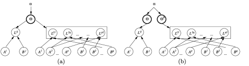
Figure 2: The score of a new data point $\{A^{i},B^{j}\}$ is given by the Bayes factor that compares models (a) and (b). Node $\alpha$ represents the hyperparameters for $\Theta$. In (a), the generative model is the same for both the new point and the query set represented in the rectangle. Notice that our conditioning set $\mathbf{S}$ of pairs might contain repeated instances of a same point, that is, some $A$ or $B$ might appear multiple times in different relations, as illustrated by nodes with multiple outgoing edges. In (b), the new point and the query set do not share the same parameters.

Thus, each pair $(A^{i},B^{j})$ is evaluated with respect to a query set $\mathbf{S}$ by the score function given in (4), rewritten after taking a logarithm and dropping constants as

$$\operatorname{score}(A^{i},B^{j}) = \log P(L^{ij}=1|X^{ij},\mathbf{S},\mathbf{L^{S}}=1)$$

$${}-\log P(L^{ij}=1|X^{ij}).$$

The exact details of our procedure are as follows. We are given a relational database $(\mathcal{D}_{A},\mathcal{D}_{B},\mathcal{L}_{AB}$). Dataset $\mathcal{D}_{A}$ ($\mathcal{D}_{B}$) is a sample of objects of type $\mathcal{A}$ ($\mathcal{B}$). Relationship table $\mathcal{L}_{AB}$ is a binary matrix modeled as generated from a logistic regression model of link existence. A query proceeds according to the following steps:

1. the user selects a set of pairs $\mathbf{S}$ that are linked in the database, where the pairs in $\mathbf{S}$ are assumed to have some relation of interest;

2. the system performs Bayesian inference to obtain the corresponding posterior distribution for $\Theta$, $P(\Theta|\mathbf{S},\mathbf{L^{S}})$, given a Gaussian prior $P(\Theta)$;

3. the system iterates through all linked pairs, computing the following for each pair:

   $$P(L^{ij}=1|X^{ij},\mathbf{S},\mathbf{L^{S}}=1)=\int P(L^{ij}=1|X^{ij},\Theta)P(\Theta|\mathbf{S},\mathbf{L^{S}}=1)\,d\Theta.$$

   $P(L^{ij}=1|X^{ij})$ is similarly computed by integrating over $P(\Theta)$. All pairs are presented in decreasing order according to the score in equation (3.1).

The integral presented above does not have a closed formula. Because computing the integrals by a Monte Carlo method for a large number of pairs would be unreasonable, we use a variational approximation [Jordan et al. (1999); Airoldi (2007)]. Figure 3 presents a summary of the approach.

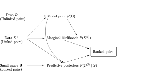
Figure 3: General framework of the procedure: first, a “prior” over parameters $\Theta$ for a link classifier is defined empirically using linked and unlinked pairs of points (the dashed edges indicate that creating a prior empirically is optional, but in practice we rely on this method). Given a query set $\mathbf{S}$ of linked pairs of interest, the system computes the predictive likelihood of each linked pair $\mathcal{D}^{(i)}\in\mathcal{D}^{+}$ and compares it to the conditional predictive likelihood, given the query. This defines a measure of similarity with respect to $\mathbf{S}$ by which all pairs in $\mathcal{D}^{+}$ are sorted.

The suggested setup scales as $O(K^{3})$ with the feature space dimension, due to the matrix inversions necessary for (variational) Bayesian logistic regression [Jaakkola and Jordan (2000)]. A less precise approximation to $P(\Theta|\mathbf{S},\mathbf{L^{S}})$ can be imposed if the dimensionality of $\Theta$ is too high. However, it is important to point out that once the initial integral $P(\Theta|\mathbf{S},\mathbf{L}^{\mathbf{S}})$ is approximated, each score function can be computed at a cost of $O(K^{2})$.

Our analogical reasoning formulation is a relational model in that it models the presence and absence of interactions between objects. By conditioning on the link indicators, the similarity score between $A\dvtx B$ and $C\dvtx D$ is always a function of pairs $(A,B)$ and $(C,D)$ that is not in general decomposable as similarities between $A$ and $C$, and $B$ and $D$.

3.2 Comparison with Bayesian sets and stochastic block models

The model presented in Figure 2 is a conditional independence model for relationship indicators, that is, given object features and parameters, the entries of $\mathcal{L}_{D}$ are independent. However, the entries in $\mathcal{L}_{D}$ are in general marginally dependent. Since this is a model of relationships given object attributes, we call the model introduced here the relational Bayesian sets model.

Our approach has some similarity to the so-called stochastic block models. These models were developed four decades ago in the network literature to quantify the notion of “structural equivalence” by means of blocks nodes that instantiate similar connectivity patterns [Lorrain and White (1971); Holland and Leinhardt (1975)]. Modern stochastic block model approaches, in statistics and machine learning, build on these seminal works by introducing the discovery of the block structure as part of the model search strategy [Fienberg, Meyer and Wasserman (1985); Nowicki and Snijders (2001); Kemp et al. (2006); Xu et al. (2006); Airoldi et al. (2005, 2008); Hoff (2008)]. The observed features in our approach, $X^{ij}$, effectively play the same role as the latent indicators in stochastic block models. Since $X^{ij}$ is observed, there is no need to integrate over the feature space to obtain the posterior distribution of $\Theta$. This computational efficiency is particularly relevant in information retrieval and exploratory data analysis, where users expect a relatively short response time.

As an alternative to our relational Bayesian sets approach, consider the following direct modification of the standard Bayesian sets formulation to this problem: merge the data sets $\mathcal{D}_{A}$ and $\mathcal{D}_{B}$ into a single data set, creating for each pair $(A^{i},B^{j})$ a row in the database with an extra binary indicator of relationship existence. Create a joint model for pairs by using the marginal models for $\mathcal{A}$ and $\mathcal{B}$ and treating different rows as being independent. This ignores the fact that the resulting merged data points are not really i.i.d. under such a model, because the same object might appear in multiple relations [Džeroski and Lavrač (2001)]. The model also fails to capture the dependency between $A^{i}$ and $B^{j}$ that arises from conditioning on $L^{ij}$, even if $A^{i}$ and $B^{j}$ are marginally independent. Nevertheless, heuristically this approach can sometimes produce good results, and for several types of probability families it is very computationally efficient. We evaluate it in Section 4.

3.3 Choice of features and relational discrimination

Our setup assumes that the feature space $\Phi$ provides a reasonable classifier to predict the existence of links. Useful predictive features can also be generated automatically with a variety of algorithms [e.g., the “structural logistic regression” of Popescul and Ungar (2003)]. See also Džeroski and Lavrač (2001). Jensen and Neville (2002) discuss shortcomings of methods for automated feature selection in relational classification.

We also assume feature spaces are the same for all possible combinations of objects. This allows for comparisons between, for example, cells from different species, or web pages from different web domains, as long as features are generated by the same function $\Phi(\cdot,\cdot)$. In general, we would like to relax this requirement, but for the problem to be well-defined, features from the different spaces must be related somehow. A hierarchical Bayesian formulation for linking different feature spaces is one possibility which might be treated in a future work.

3.4 Priors

The choice of prior is based on the observed data, in a way that is equivalent to the choice of priors used in the original formulation of Bayesian sets [Ghahramani and Heller (2005)]. Let $\widehat{\Theta}$ be the maximum likelihood estimator of $\Theta$ using the relational database $(\mathcal{D}_{A},\mathcal{D}_{B},\mathcal{L}_{AB})$. Since the number of possible pairs grows at a quadratic rate with the number of objects, we do not use the whole database for maximum likelihood estimation. Instead, to get $\widehat{\Theta}$, we use all linked pairs as members of the “positive” class ($L=1$), and subsample unlinked pairs as members of the “negative” class ($L=0$). We subsample by sampling each object uniformly at random from the respective data sets $\mathcal{D}_{A}$ and $\mathcal{D}_{B}$ to get a new pair. Since link matrices $\mathcal{L}_{AB}$ are usually very sparse, in practice, this will almost always provide an unlinked pair. Sections 4 and 5 provide more details.

We use the prior $P(\Theta)=\mathcal{N}(\widehat{\Theta},(c\widehat{\mathbf{T}})^{-1}$), where $\mathcal{N}(\mathbf{m},\mathbf{V})$ is a normal of mean $\mathbf{m}$ and variance $\mathbf{V}$. Matrix $\widehat{\mathbf{T}}$ is the empirical second moments matrix of the linked object features, although a different choice might be adequate for different applications. Constant $c$ is a smoothing parameter set by the user. In all of our experiments we set $c$ to be equal to the number of positive pairs. A good choice of $c$ might be important to obtain maximum performance, but we leave this issue as future work. Wang et al. (2009) present some sensitivity analysis results for a particular application in text analysis.

Empirical priors are a sensible choice, since this is a retrieval, not a predictive, task. Basically, the entire data set is the population, from which prior information is obtained on possible query sets. A data-dependent prior based on the population is important for an approach such as Bayesian sets, since deviances from the “average” behavior in the data are useful to discriminate between subpopulations.

3.5 On continuous and multivariate relations

Although we focus on measuring similarity of qualitative relationships, the same idea could be extended to continuous (or ordinal) measures of relationship, or relationships where each $L^{ij}$ is a vector. For instance, Turney and Littman (2005) measure relations between words by their co-occurrences on the neighborhood of specific keywords, such as the frequency of two words being connected by a specific preposition in a large body of text documents. Several similarity metrics can be defined on this vector of continuous relationships. However, given data on word features, one can easily modify our approach by substituting the logistic regression component with some multiple regression model.

4 Ranking hyperlinks on the web

In the following application we consider a collection of web pages from several universities: the WebKB collection, where relations are given by hyperlinks [Craven et al. (1998)]. Web pages are classified as being of type course, department, faculty, project, staff, student or other. Documents come from four universities (Cornell, Texas, Washington and Wisconsin). We are interested in recovering pairs of web pages $\{A,B\}$ where web page $A$ has a link to web page $B$. Notice that the relationship is asymmetric. Different types of web pages imply different types of links. For instance, a faculty web page linking to a project web page constitutes a type of link. The analogical reasoning task here is simplified if we assume each web page object has a single role (i.e., exactly one out of the pre-defined types {course, department, faculty, project, staff, student, other}), and therefore a pair of web pages implies a unique type of relationship. The web page types are for evaluation purposes only, as we explain later: we will not provide this information to the model.

Our main standard of comparison is a “flattened Bayesian sets” algorithm (which we will call “standard Bayesian sets,” SBSets, in constrast to the relational model, RBSets). Using a multivariate independent Bernoulli model as in the original paper [Ghahramani and Heller (2005)], we merge linked web page pairs into single rows, and then apply the original algorithm directly to the merged data. It is clear that data points are not independent anymore, but the SBSets algorithm assumes this is the case. Evaluating this algorithm serves the purpose of both measuring the loss of not treating relational data as such, as well as the limitations of evaluating the similarity of pairs through models for the marginal probabilities of $\mathcal{A}$ and $\mathcal{B}$ instead of models for the predictive function $P(L^{ij}|X^{ij})$.

Binary data was extracted from this database using the same methodology as in Ghahramani and Heller (2005). A total of 19,450 binary variables per object are generated, where each variable indicates whether a word from a fixed dictionary appears in a given document more frequently than the average. To avoid introducing extra approximations into RBSets, we reduced the dimensionality of the original representation using singular value decomposition, obtaining 25 measures per object.

In this experiment objects are of the same type, and therefore, dimensionality. The feature vector $X^{ij}$ for each pair of objects $\{A^{i},B^{j}\}$ consists of the $V$ features for object $A^{i}$, the $V$ features of object $B^{j}$, and measures $\mathbf{Z}=\{Z_{1},\ldots,Z_{V}\}$, where $Z_{v}=(A^{i}_{v}\times B^{j}_{v})/(|A^{i}|\times\|B^{j}\|)$, $\|A^{i}\|$ being the Euclidean norm of the $V$-dimensional representation of $A^{i}$. We also add a constant value (1) to the feature set as an intercept term for the logistic regression. Feature set $\mathbf{Z}$ is exactly the one used in the cosine distance measure, a common and practical measure widely used in information retrieval [Manning, Raghavan and Schütze (2008)]. This feature space also has the important advantage of scaling well (linearly) with the number of variables in the database. Moreover, adopting such features will make our comparisons fairer, since we evaluate how well cosine distance itself performs in our task. Notice that our choice of $X^{ij}$ is suitable for asymmetric relationships, as naturally occurs in the domain of web page links. For symmetric relationships, features such as $|A^{i}_{v}-B^{j}_{v}|$ could be used instead.

In order to set the empirical prior, we sample 10 “negative” pairs for each “positive” one, and weight them to reflect the proportion of linked to unlinked pairs in the database. That is, in the WebKB study we use 10 negatives for each positive, and we count each negative case as being 350 cases replicated. We perform subsampling and reweighting in order to be able to fit the database in the memory of a desktop computer.

Evaluation of the significance of retrieved items often relies on subjective assessments [Ghahramani and Heller (2005)]. To simplify our study, we will focus on particular setups where objective measures of success are defined.

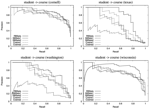
Figure 4: Results for student $\rightarrow$ course relationships.

To evaluate the gain of our model over competitors, we will use the following setup. In the first query, we are given all pairs of web pages of the type student $\rightarrow$ course from three of the labeled universities, and evaluate how relations are ranked in the fourth university. Because we know class labels for the web pages (while the algorithm does not), we can use the classes of the returned pairs to label a hit as being “relevant” or “irrelevant.” We label a pair $(A^{i},B^{j})$ as relevant if and only if $A^{i}$ is of type student and $B^{j}$ is of type course, and $A^{i}$ links to $B^{j}$.

This is a very stringent criterion, since other types of relations could also be valid (e.g., staff $\rightarrow$ course appears to be a reasonable match). However, this facilitates objective comparisons of algorithms. Also, the other class contains many types of pages, which allows for possibilities such as a student $\rightarrow$ “hobby” pair. Such pairs might be hard to evaluate (e.g., is that particular hobby demanding or challenging in a similar way to coursework?). As a compromise, we omit all pages from the category other in order to better clarify differences between algorithms.

Precision/recall curves [Manning, Raghavan and Schütze (2008)] for the student $\rightarrow$ course queries are shown in Figure 4. There are four queries, each corresponding to a search over a specific university given all valid student $\rightarrow$ course pairs from the other three. There are four algorithms on each evaluation: the standard Bayesian sets with the original 19,450 binary variables for each object, plus another 19,450 binary variables, each corresponding to the product of the respective variables in the original pair of objects (SBSets1); the standard Bayesian sets with the original binary variables only (SBSets2); a standard cosine distance measure over the 25-dimensional representation (Cosine 1) for each page, with pairs being given by the combined vector of 50 features; a cosine distance measure using the raw 19,450-dimensional binary for each document (Cosine 2); our approach, RBSets.

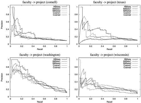
Figure 5: Results for faculty $\rightarrow$ project relationships.

In Figure 4 RBSets demonstrates consistently superior or equal precision-recall. Although SBSets performs well when asked to retrieve only student items or only course items, it falls short of detecting what features of student and course are relevant to predict a link. The discriminative model within RBSets conveys this information through the link parameters.

We also did an experiment with a query of type faculty $\rightarrow$ project, shown in Figure 5. This time results between algorithms were closer to each other. To make differences more evident, we adopt a slightly different measure of success: we count as a 1 hit if the pair retrieved is a faculty $\rightarrow$ project pair, and count as a 0.5 hit for pairs of type student $\rightarrow$ project and staff $\rightarrow$ project. Notice this is a much harder query. For instance, the structure of the project web pages in the texas group was quite distinct from the other universities: they are mostly very short, basically containing links for members of the project and other project web pages.

Although the precision/recall curves convey a global picture of the performance of each algorithm, they might not be a completely clear way of ranking approaches for cases where curves intersect at several points. In order to summarize algorithm performances with a single statistic, we computed the area under each precision/recall curve (with linear interpolation between points). Results are given in Table 1. Numbers in bold indicate the largest area under the curve. The dominance of RBSets should be clear.

Table 1: Area under the precision/recall curve for each algorithm and query

	Student $\bolds{\rightarrow}$ course					Faculty $\bolds{\rightarrow}$ project
	C1	C2	RB	SB1	SB2	C1	C2	RB	SB1	SB2
Cornell	0.87	0.82	0.87	0.82	0.80	0.19	0.18	0.24	0.18	0.18
Texas	0.62	0.32	0.77	0.55	0.54	0.24	0.21	0.29	0.12	0.12
Washington	0.69	0.31	0.76	0.67	0.64	0.40	0.42	0.47	0.40	0.40
Wisconsin	0.77	0.72	0.88	0.75	0.73	0.28	0.30	0.26	0.19	0.21

5 Ranking protein interactions

The budding yeast is a unicellular organism that has become a de-facto model organism for the study of molecular and cellular biology [Botstein, Chervitz and Cherry (1997)]. There are about 6000 proteins in the budding yeast, which interact in a number of ways [Cherry et al. (1997)]. For instance, proteins bind together to form protein complexes, the physical units that carry out most functions in the cell [Krogan et al. (2006)]. In recent years, significant resources have been directed to collect experimental evidence of physical proteins binding, in an effort to infer and catalogue protein complexes and their multifaceted functional roles [e.g., Fields and Song (1989); Itô et al. (2000); Uetz et al. (2000); Gavin et al. (2002); Ho et al. (2002)]. Currently, there are four main sources of interactions between pairs of proteins that target proteins localized in different cellular compartments with variable degrees of success: (i) literature curated interactions [Reguly et al. (2006)], (ii) yeast two-hybrid (Y2H) interaction assays [Yu et al. (2008)], (iii) protein fragment complementation (PCA) interaction assays [Tarassov et al. (2008)], and (iv) tandem affinity purification (TAP) interaction assays [Gavin et al. (2006); Krogan et al. (2006)]. These collections include a total of about 12,292 protein interactions [Jensen and Bork (2008)], although the number of such interactions is estimated to be between 18,000 [Yu et al. (2008)] and 30,000 [von Mering et al. (2002)].

Statistical methods have been developed for analyzing many aspects of this large protein interaction network, including de-noising [Bernard, Vaughn and Hartemink (2007); Airoldi et al. (2008)], function prediction [Nabieva et al. (2005)] and identification of binding motifs [Banks et al. (2008)].

5.1 Overview of the analysis

We consider multiple functional categorization systems for the proteins in budding yeast. For evaluation purposes, we use individual proteins’ functional annotations curated by the Munich Institute for Protein Sequencing [MIPS, Mewes et al. (2004)], those by the Kyoto Encyclopedia of Genes and Genomes [KEGG, Kanehisa and Goto (2000)] and those by the Gene Ontology consortium [GO, Ashburner et al. (2000)]. We consider multiple collections of physical protein interactions that encode alternative semantics. Physical protein-to-protein interactions in the MIPS curated collection measure physical binding events observed experimentally in Y2H and TAP experiments, whereas physical protein-to-protein interactions in the KEGG curated collection measure a number of different modes of interactions, including phosporelation, methylation and physical binding, all taking place in the context of a specific signaling pathway. So we have three possible functional annotation databases (MIPS, KEGG and GO) and two possible link matrices (MIPS and KEGG), which can be combined.

Our experimental pipeline is as follows: (i) Pick a database of functional annotations, say, MIPS, and a collection of interactions, say, MIPS (again). (ii) Pick a pair of categories, $M_{1}$ and $M_{2}$. For instance, take $M_{1}$ to be cytoplasm (MIPS 40.03) and $M_{2}$ to be cytoplasmic and nuclear degradation (MIPS 06.13.01). (iii) Sample, uniformly at random and without replacement, a set $\mathbf{S}$ of 15 interactions in the chosen collection. (iv) Rank other interacting pairs according to the score in equation (3.1) and, for comparison purposes, according to three other approaches to be described in Section 5.1.4. (v) The process is repeated for a large number of pairs $M_{1}\times M_{2}$, and 5 different query sets $\mathbf{S}$ are generated for each pair of categories. (vi) Calculate an evaluation metric for each query and each of the four scores, and report a comparative summary of the results.

Table 2: Collection of data sets used to generate protein-specific features

No.	Measurements description	Data sources
1.	Expression microarrays	Gasch et al. (2000); Brem et al. (2005);
		Primig et al. (2000); Yvert et al. (2003)
2.	Synthetic genetic interactions	Breitkreutz, Stark and Tyers (2003); SGD
3.	Cellular localization	Huh et al. (2003)
4.	Transcription factor binding sites	Harbison et al. (2004); TRANSFAC
5.	Sequence similarities	Altschul et al. (1990); Zhu and Zhang (1999)

5.1.1 Protein-specific features

The protein-specific features were generated using the data sets summarized in Table 2 and an additional data set [Qi, Bar-Joseph and Klein-Seetharaman (2006)]. Twenty gene expression attributes were obtained from the data set processed by Qi, Bar-Joseph and Klein-Seetharaman (2006). Each gene expression attribute for a protein pair $P_{i}\dvtx P_{j}$ corresponds to the correlation coefficient between the expression levels of corresponding genes. The 20 different attributes are obtained from 20 different experimental conditions as measured by microarrays. We did not use pairs of proteins from Qi et al. for which we did not have data in the data sets listed in Table 2. This resulted in approximately 6000 positively linked data points for the MIPS network and 39,000 for KEGG.

We generated another 25 protein–protein gene expression features from the data in Table 2 using the same procedure based on correlation coefficients. This gives a total of 45 attributes, corresponding to the main data set used in our relational Bayesian sets runs.

Another data set was generated using the remaining (i.e., nonmicroarray) features of Table 2. Such features are binary and highly sparse, with most entries being 0 for the majority of linked pairs. We removed attributes for which we had fewer than 20 linked pairs with positive values according to the MIPS network. The total number of extra binary attributes was 16.

Several measurements were missing. We imputed missing values for each variable in a particular data point by using its empirical average among the observed values.

Given the 45 or 61 attributes of a given pair {$P_{i}$, $P_{j}$}, we applied a nonlinear transformation where we normalize the vector by its Euclidean norm in order to obtain our feature table $\mathbf{X}$.

5.1.2 Calibrating the prior for $\Theta$

We initially fit a logistic regression classifier using a maximum likelihood estimation (MLE) and our data, obtaining the estimate $\widehat{\Theta}$. Our choice of covariance matrix $\widehat{\Sigma}$ for $\Theta$ is defined to be a rescaling of a squared norm of the data:

$$(\widehat{\Sigma})^{-1}=\mathbf{X}^{\mathsf{T}}_{\mathrm{POS}}\mathbf{X}_{\mathrm{POS}},$$ (6)

where $\mathbf{X}_{\mathrm{POS}}$ is the matrix containing the protein–protein features only of the linked pairs used in the MLE computation.

5.1.3 Evaluation metrics

As in the WebKB experiment, we propose an objective measure of evaluation that is used to compare different algorithms. Consider a query set $\mathbf{S}$, and a ranked response list $\mathbf{R}=\{R^{1},R^{2},R^{3},\ldots,R^{N}\}$ of protein–protein pairs. Every element of $\mathbf{S}$ is a pair of proteins $P_{i}\dvtx P_{j}$ such that $P_{i}$ is of class $M_{i}$ and $P_{j}$ is of class $M_{j}$, where $M_{i}$ and $M_{j}$ are classes from either MIPS, KEGG or Gene Ontology. In general, proteins belong to multiple classes. This is in contrast with the WebKB experiment, where, according to our web page categorization, there was only one possible type of relationship for each pair of web pages. The retrieval algorithm that generates $\mathbf{R}$ does not receive any information concerning the MIPS, KEGG or GO taxonomy. $\mathbf{R}$ starts with the linked protein pair that is judged most similar to $\mathbf{S}$, followed by the other protein pairs in the population, in decreasing order of similarity. Each algorithm has its own measure of similarity.

The evaluation criterion for each algorithm is as follows: as before, we generate a precision-recall curve and calculate the area under the curve (AUC). We also calculate the proportion (TOP10), among the top 10 elements in each ranking, of pairs that match the original $\{M_{1},M_{2}\}$ selection (i.e., a “correct” $P_{i}\dvtx P_{j}$ is one where $P_{i}$ is of class $M_{1}$ and $P_{j}$ of class $M_{2}$, or vice-versa. Notice that each protein belongs to multiple classes, so both conditions might be satisfied.) Since a researcher is only likely to look at the top ranked pairs, it makes sense to define a measure that uses only a subset of the ranking. AUC and TOP10 are our two evaluation measures.

The original classes $\{M_{1},M_{2}\}$ are known to the experimenter but not known to the algorithms. As in the WebKB experiment, our criterion is rather stringent, in the sense that it requires a perfect match of each $R^{I}$ with the MIPS, KEGG or GO categorization. There are several ways by which a pair $R^{I}$ might be analogous to the relation implicit in $\mathbf{S}$, and they do not need to agree with MIPS, GO or KEGG. Still, if we are willing to believe that these standard categorization systems capture functional organization of proteins at some level, this must lead to association between categories given to $\mathbf{S}$ and relevant subpopulations of protein–protein interactions similar to $\mathbf{S}$. Therefore, the corresponding AUC and TOP10 are useful tools for comparing different algorithms even if the actual measures are likely to be pessimistic for a fixed algorithm.

5.1.4 Competing algorithms

We compare our method against a variant of it and two similarity metrics widely used for information retrieval:

1. The cosine score [Manning, Raghavan and Schütze (2008)], denoted by cos.

2. The nearest neighbor score, denoted by nns.

3. The relational maximum likelihood sets score, denoted by mls.

The nearest neighbor score measures the minimum Euclidean distance between $R^{I}$ and any individual point in $\mathbf{S}$, for a given query set $\mathbf{S}$ and a given candidate point $R^{I}$. The relational maximum likelihood sets is a variation of RBSets where we initially sample a subset of the unlinked pairs (10,000 points in our setup) and, for each query $\mathbf{S}$, we fit a logistic regression model to obtain the parameter estimate $\Theta_{\mathbf{S}}^{\mathrm{MLE}}$. We also use a logistic regression model fit to the whole data set (the same one used to generate the prior for RBSets), giving the estimate $\Theta^{\mathrm{MLE}}$. A new score, analogous to (3.1), is given by $\log P(L^{ij}=1|X^{ij},\Theta_{\mathbf{S}}^{\mathrm{MLE}})-\log P(L^{ij}=1|X^{ij},\Theta^{\mathrm{MLE}})$, that is, we do not integrate out the parameters or use a prior, but instead the models are fixed at their respective estimates.

Neither cos or nns can be interpreted as measures of analogical similarity, in the sense that they do not take into account how the protein pair features $\mathbf{X}$ contribute to their interaction. It is true that a direct measure of analogical similarity is not theoretically required to perform well according to our (nonanalogical) evaluation metric. However, we will see that there are practical advantages in doing so.

5.2 Results on the MIPS collection of physical interactions

For this batch of experiments, we use the MIPS network of protein–protein interactions to define the relationships. In the initial experiment, we selected queries from all combinations of MIPS classes for which there were at least 50 linked pairs $P_{i}\dvtx P_{j}$ in the network that satisfied the choice of classes. Each query set contained 15 pairs. After removing the MIPS-categorized proteins for which we had no feature data, we ended up with a total of 6125 proteins and 7788 positive interactions. We set the prior for RBSets using a sample of 225,842 pairs labeled as having no interaction, as selected by Qi, Bar-Joseph and Klein-Seetharaman (2006).

For each tentative query set $\mathbf{S}$ of categories $\{M_{1},M_{2}\}$, we scored and ranked pairs $P_{i}^{\prime}\dvtx P_{j}^{\prime}$ such that both $P_{i}^{\prime}$ and $P_{j}^{\prime}$ were connected to some protein appearing in $\mathbf{S}$ by a path of no more than two steps, according to the MIPS network. The reasons for the filtering are two-fold: to increase the computational performance of the ranking since fewer pairs are scored; and to minimize the chance that undesirable pairs would appear in the top 10 ranked pairs. Tentative queries would not be performed if after filtering we obtained fewer than 50 possible correct matches. Trivial queries, where filtering resulted only in pairs in the same class as the query, were also discarded. The resulting number of unique pairs of categories $\{M_{1},M_{2}\}$ was 931 classes of interactions. For each pair of categories, we sampled our query set $\mathbf{S}$ 5 times, generating a total of 4655 rankings per algorithm.

Table 3: Number of times each method wins when querying pairs of MIPS classes using the MIPS protein–protein interaction network. The first two columns, #AUC and #TOP10, count the number of times the respective method obtains the best score according to the AUC and TOP10 measures, respectively, among the 4 approaches. This is divided by the number of replications of each query type (5). The last two columns, #AUC.S and #TOP10.S, are “smoothed” versions of this statistic: a method is declared the winner of a round of 5 replications if it obtains the best score in at least 3 out of the 5 replications. The top table shows the results when only the continuous variables are used by RBSets, and in the bottom table when the discrete variables are also given to RBSets

Method	#AUC	#TOP10	#AUC.S	#TOP10.S
(a)
COS	240	294	219	277
NNS	042	122	028	075
MLS	105	270	052	198
RBSets	542	556	578	587
(b)
COS	314	356	306	340
NNS	075	146	062	111
MLS	273	329	246	272
RBSets	267	402	245	387

Table 4: Pairwise comparison of methods according to the AUC and TOP10 criterion.Each cell shows the proportion of the trials where the method in the respective row wins over the method in the column, according to both criteria. In each cell, the proportion is calculated with respect to the 4655 rankings where no tie happened

	AUC				TOP10
	COS	NNS	MLS	RBSets	COS	NNS	MLS	RBSets
COS	–	0.67	0.43	0.30	–	0.70	0.46	0.30
NNS	0.32	–	0.18	0.06	0.29	–	0.25	0.11
MLS	0.56	0.81	–	0.25	0.53	0.74	–	0.28
RBSets	0.69	0.93	0.74	–	0.69	0.88	0.71	–

We run two types of experiments. In one version, we give to RBSets the data containing only the 45 (continuous) microarray measurements. In the second variation, we provide to RBSets all 61 variables, including the 16 sparse binary indicators. However, we noticed that the addition of the 16 binary variables hurts RBSets considerably. We conjecture that one reason might be the degradation of the variational approximation. Including the binary variables hardly changed the other three methods, so we choose to use the 61 variable data set for the other methods.

Table 3 summarizes the results of this experiment. We show the number of times each method wins according to both the AUC and TOP10 criteria. The number of wins is presented as divided by 5, the number of random sets generated for each query type $\{M_{1},M_{2}\}$ (notice these numbers do not need to add up to 931, since ties are possible). Moreover, we also presented “smoothed” versions of this statistic, where we count a method as the winner for any given $\{M_{1},M_{2}\}$ category if, for the group of 5 queries, the method obtains the best result in at least 3 of the sets. The motivation is to smooth out the extra variability added by the particular set of 15 protein pairs for a fixed $\{M_{1},M_{2}\}$. The proposed relational Bayesian sets method is the clear winner according to all measures when we select only the continuous variables. For this reason, for the rest of this section all analysis and experiments will consider only this case.

Table 4 displays a pairwise comparison of the methods. In this table we show how often the row method performs better than the column method, among those trials where there was no tie. Again, RBSets dominates.

Another useful summary is the distribution of correct hits in the top 10 ranked elements across queries. This provides a measure of the difficulty of the problem, besides the relative performance of each algorithm. In Table 5 we show the proportion of correct hits among the top 10 for each algorithm for our queries using MIPS categorization and also GO categorization, as explained in the next section. About 14% of the time, all pairs in the top 10 pairs ranked by RBSets were of the intended type, compared to 8% of the second best approach.

Table 5: Distribution across all queries of the number of hits in the top 10 pairs,as ranked by each algorithm. The more skewed to the right, the better. Notice that using GO categories doubles the number of zero hits for RBSets

	0	1	2	3	4	5	6	7	8	9	10
Proportion of top hits using MIPS categories and links specified by the MIPS database
COS	0.12	0.15	0.12	0.10	0.08	0.07	0.06	0.05	0.04	0.07	0.08
NNS	0.29	0.16	0.14	0.10	0.06	0.05	0.03	0.03	0.03	0.03	0.02
MLS	0.12	0.12	0.12	0.10	0.09	0.08	0.07	0.06	0.07	0.06	0.07
RBSets	0.04	0.08	0.09	0.09	0.09	0.08	0.09	0.07	0.09	0.08	0.14
Proportion of top hits using GO categories and links specified by the MIPS database
COS	0.12	0.13	0.11	0.10	0.11	0.09	0.06	0.06	0.04	0.06	0.06
NNS	0.53	0.23	0.07	0.02	0.02	0.02	0.04	0.01	0.00	0.00	0.01
MLS	0.16	0.11	0.12	0.10	0.08	0.08	0.08	0.06	0.05	0.06	0.05
RBSets	0.09	0.09	0.10	0.10	0.08	0.08	0.06	0.08	0.08	0.07	0.12

Table 6: Number of times each method wins when querying pairs of GO classes using the MIPS protein–protein interaction network. Columns #AUC, #TOP10, #AUC.S and #TOP10.S are defined as in Table 3

Method	#AUC	#TOP10	#AUC.S	#TOP10.S
COS	58	073	058	072
NNS	01	010	000	004
MLS	26	055	013	038
RBSets	93	.105	.101	110

5.2.1 Changing the categorization system

A variation of this experiment was performed where the protein categorizations do not come from the same family as the link network, that is, where we used the MIPS network but not the MIPS categorization. Instead we performed queries according to the Gene Ontology categories. Starting from 150 pre-selected GO categories [Myers et al. (2006)], we once again generated unordered category pairs $\{M_{1},M_{2}\}$. A total of 179 queries, with 5 replications each (a total of 895 rankings), were generated and the results summarized in Table 6.

This is a more challenging scenario for our approach, which is optimized with respect to MIPS. Still, we are able to outperform other approaches. Differences are less dramatic, but consistent. In the pairwise comparison of RBSets against the second best method, cos, our method wins 62% of the time by the TOP10 criterion.

5.2.2 The role of filtering

In both experiments with the MIPS network, we filtered candidates by examining only a subset of the proteins linked to the elements in the query set by a path of no more than two proteins. It is relevant to evaluate how much coverage of each category pair $\{M_{1},M_{2}\}$ we obtain by this neighborhood selection.

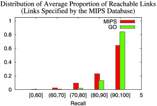
Figure 6: Distribution of the coverage of valid pairs in the MIPS network, according to our generated query sets. Results are broken into the two categorization systems (MIPS and GO) used in this experiment.

For each query $\mathbf{S}$, we calculate the proportion of pairs $P_{i}\dvtx P_{j}$ of the same categorization $\{M_{1},M_{2}\}$ such that both $P_{i}$ and $P_{j}$ are included in the neighborhood. Figure 6 shows the resulting distributions of such proportions (from 0 to 100%): a histogram for the MIPS search and a histogram for the GO search. Despite the small neighborhood, coverage is large. For the MIPS categorization, 93% of the queries resulted in a coverage of at least 75% (with 24% of the queries resulting in perfect coverage). Although filtering implies that some valid pairs will never be ranked, the gain obtained by reducing false positives in the top 10 ranked pairs is considerable (results not shown) across all methods, and the computational gain of reducing the search space is particularly relevant in exploratory data analysis.

5.3 Results on the KEGG collection of signaling pathways

We repeat the same experimental setup, now using the KEGG network to define the protein–protein interactions. We selected proteins from the KEGG categorization system for which we had data available. A total of 6125 proteins were selected. The KEGG network is much more dense than MIPS. A total of 38,961 positive pairs and 226,188 negative links were used to generate our empirical prior.

However, since the KEGG network is much more dense than MIPS, we filtered our candidate pairs by allowing only proteins that are directly linked to the proteins in the query set $\mathbf{S}$. Even under this restriction, we are able to obtain high coverage: the neighborhood of 90% of the queries included all valid pairs of the same category, and essentially all queries included at least 75% of the pairs falling in the same category as the query set. A total of 1523 possible pairs of categories (7615 queries, considering the 5 replications) were generated.

Table 7: Number of times each method wins when querying pairs of KEGG classes using the KEGG protein–protein interaction network. Columns #AUC, #TOP10, #AUC.S and #TOP10.S are defined as in Table 3

Method	#AUC	#TOP10	#AUC.S	#TOP10.S
COS	0159	0575	0134	0507
NNS	0030	0305	0017	0227
MLS	0290	0506	0199	0431
RBSets	1042	1091	1107	1212

Table 8: Distribution across all queries of the number of hits in the top 10 pairs, as ranked by each algorithm. The more skewed to the right, the better

	0	1	2	3	4	5	6	7	8	9	10
Proportion of top hits using KEGG categories and links specified by the KEGG database
COS	0.56	0.21	0.08	0.03	0.02	0.01	0.01	0.01	0.01	0.01	0.01
NNS	0.89	0.03	0.04	0.01	0.00	0.00	0.00	0.00	0.00	0.00	0.00
MLS	0.57	0.21	0.08	0.04	0.02	0.01	0.01	0.00	0.00	0.00	0.00
RBSets	0.29	0.24	0.16	0.09	0.06	0.03	0.02	0.01	0.03	0.02	0.01

Results are summarized in Table 7. Again, it is evident that RBSets dominates other methods. In the pairwise comparison against cos, RBSets wins 76% of the times according to the TOP10 criterion. However, the ranking problem in the KEGG network was much harder than in the MIPS network (according to our automated nonanalogical criterion). We believe that the reason is that, in KEGG, the simple filtering scheme has much less influence as reflected by the high coverage. The distribution of the number of hits in the top 10 ranked items is shown in Table 8. Despite the success of RBSets relative to the other algorithms, there is room for improvement.

6 More related work

There is a large literature on analogical reasoning in artificial intelligence and psychology. We refer to French (2002) for a survey, and to more recent papers on clustering [Marx et al. (2002)], prediction [Turney and Littman (2005); Turney (2008a)] and dimensionality reduction [Memisevic and Hinton (2005)] as examples of other applications. Classical approaches for planning have also exploited analogical similarities [Veloso and Carbonell (1993)].

Nonprobabilistic similarity functions between relational structures have also been developed for the purpose of deriving kernel matrices, such as those required by support vector machines. Borgwardt (2007) provides a comprehensive survey and state-of-the-art methods. It would be interesting to adapt such methods to problems of analogical reasoning.

The graphical model formulation of Getoor et al. (2002) incorporates models of link existence in relational databases, an idea used explicitly in Section 3 as the first step of our problem formulation. In the clustering literature, the probabilistic approach of Kemp et al. (2006) is motivated by principles similar to those in our formulation: the idea is that there is an infinite mixture of subpopulations that generates the observed relations. Our problem, however, is to retrieve other elements of a subpopulation described by elements of a query set, a goal that is closer to the classical paradigm of analogical reasoning.

As discussed in Section 3.2, our model can be interpreted as a type of block model [Kemp et al. (2006); Xu et al. (2006); Airoldi et al. (2008)] with observable features. Link indicators are independent given the object features, which might not actually be the case for particular choices of feature space. In theory, block models sidestep this issue by learning all the necessary latent features that account for link dependence. An important future extension of our work would consist of tractably modeling the residual link association that is not accounted for by our observed features.

Discovering analogies is a specific task within the general problem of generating latent relationships from relational data. Some of the first formal methods for discovering latent relationships from multiple data sets were introduced in the literature of inductive logic programming, such as the inverse resolution method [Muggleton (1981)]. A more recent probabilistic method is discussed by Kok and Domingos (2007). Džeroski and Lavrač (2001) and Getoor and Taskar (2007) provide an overview of relational learning methods from a data mining and machine learning perspective.

A particularly active subfield on latent relationship generation lies within text analysis research. For instance, Stephens et al. (2001) describe an approach for discovering relations between genes given MEDLINE abstracts. In the context of information retrieval, Cafarella, Banko and Etzioni (2006) describe an application of recent unsupervised information extraction methods: relations generated from unstructured text documents are used as a preprocessing step to build an index of web pages. In analogical reasoning applications, our method has been used by others for question-answering analysis [Wang et al. (2009)].

The idea of measuring the similarity of two data points based on a predictive function has appeared in the literature on matching for causal inference. Suppose we are given a model for predicting an outcome $Y$ given a treatment $Z$ and a set of potential confounders $\mathbf{X}$. For simplicity, assume $Z\in\{0,1\}$. The goal of matching is to find, for each data point $(\mathbf{X}_{i},Y_{i},Z_{i})$, the closest match $(\mathbf{X}_{j},Y_{j},Z_{j})$ according to the confounding variables $\mathbf{X}$. In principle, any clustering criterion could be used in this task [Gelman and Hill (2007)]. The propensity score criterion [Rosenbaum (2002)] measures the similarity of two feature vectors $\mathbf{X}_{i}$ and $\mathbf{X}_{j}$ by comparing the predictions $P(Z_{i}=1|\mathbf{X}_{i})$ and $P(Z_{j}=1|\mathbf{X}_{j})$. If the conditional $P(Z=1|\mathbf{X})$ is given by a logistic regression model with parameter vector $\Theta$, Gelman and Hill (2007) suggest measuring the difference between $\mathbf{X}_{i}^{\mathsf{T}}\Theta$ and $\mathbf{X}_{j}^{\mathsf{T}}\Theta$. While this is not the same as comparing two predictive functions as in our framework, the core idea of using predictive functions to define similarity remains.

A preliminary version of this paper appeared in the proceedings of the 11th International Conference on Artificial Intelligence and Statistics [Silva, Heller and Ghahramani (2007)].

7 Conclusion

We have presented a framework for performing analogical reasoning within a Bayesian data analysis formulation. There is of course much more to analogical reasoning than calculating the similarity of related pairs. As future work, we will consider hierarchical models that could in principle compare relational structures (such as protein complexes) of different sizes. In particular, the literature on graph kernels [Borgwardt (2007)] could provide insights on developing efficient similarity metrics within our probabilitistic framework.

Also, we would like to combine the properties of the mixed-membership stochastic block model of Airoldi et al. (2008), where objects are clustered into multiple roles according to the relationship matrix $\mathcal{L}_{AB}$, with our framework where relationship indicators are conditionally independent given observed features.

Finally, we would like to consider the case where multiple relationship matrices are available, allowing for the comparison of relational structures with multiple types of objects.

Much remains to be done to create a complete analogical reasoning system, but the described approach has immediate applications to information retrieval and exploratory data analysis.

References

- Airoldi (2007) Airoldi, E. M. (2007). Getting started in probabilistic graphical models. PLoS Computational Biology 3 e252.
- Airoldi et al. (2005) Airoldi, E. M., Blei, D. M., Xing, E. P. and Fienberg, S. E. (2005). A latent mixed-membership model for relational data. In Workshop on Link Discovery: Issues, Approaches and Applications, in Conjunction With the 11th International ACM SIGKDD Conference. Chicago, IL.
- Airoldi et al. (2008) Airoldi, E. M., Blei, D. M., Fienberg, S. E. and Xing, E. P. (2008). Mixed membership stochastic blockmodels. J. Mach. Learn. Res. 9 1981–2014.
- Altschul et al. (1990) Altschul, S. F., Gish, W., Miller, W., Myers, E. W. and Lipman, D. J. (1990). Basic local alignment search tool. Journal of Molecular Biology 215 403–410.
- Ashburner et al. (2000) Ashburner, M., Ball, C. A., Blake, J. A., Botstein, D., Butler, H., Cherry, J. M., Davis, A. P., Dolinski, K., Dwight, S. S., Eppig, J. T., Harris, M. A., Hill, D. P., Issel-Tarver, L., Kasarskis, A., Lewis, S., Matese, J. C., Richardson, J. E., Ringwald, M., Rubinand, G. M. and Sherlock, G. (2000). Gene ontology: Tool for the unification of biology. The gene ontology consortium. Nature Genetics 25 25–29.
- Banks et al. (2008) Banks, E., Nabieva, E., Peterson, R. and Singh, M. (2008). NetGrep: Fast network schema searches in interactomes. Genome Biology 24 1473–1480.
- Bernard, Vaughn and Hartemink (2007) Bernard, A., Vaughn, D. S. and Hartemink, A. J. (2007). Reconstructing the topology of protein complexes. In Research in Computational Molecular Biology 2007 (RECOMB07) (T. Speed and H. Huang, eds.). Lecture Notes in Bioinformatics 4453 32–46. Springer, Berlin.
- Borgwardt (2007) Borgwardt, K. (2007). Graph kernels. Ph.D. thesis, Ludwig-Maximilians-Univ. Munich.
- Botstein, Chervitz and Cherry (1997) Botstein, D., Chervitz, S. A. and Cherry, J. M. (1997). Yeast as a model organism. Science 277 1259–1260.
- Breitkreutz, Stark and Tyers (2003) Breitkreutz, B. J., Stark, C. and Tyers, M. (2003). The GRID: The General Repository for Interaction Datasets. Genome Biology 4 R23.
- Brem et al. (2005) Brem, R. B., Storey, J. D., Whittle, J. and Kruglyak, L. (2005). Genetic interactions between polymorphisms that affect gene expression in yeast. Nature 436 701–703.
- Cafarella, Banko and Etzioni (2006) Cafarella, M., Banko, M. and Etzioni, O. (2006). Relational web search. Technical report 2006-04-02, Univ. Washington, Dept. Computer Science and Engineering.
- Cherry et al. (1997) Cherry, J. M., Ball, C., Weng, S., Juvik, G., Schmidt, R., Adler, C., Dunn, B., Dwight, S., Riles, L., Mortimer, R. K. and Botstein, D. (1997). Genetic and physical maps of saccharomyces cerevisiae. Nature 387 67–73.
- Craven et al. (1998) Craven, M., DiPasquo, D., Freitag, D., McCallum, A., Mitchell, T., Nigam, K. and Slattery, S. (1998). Learning to extract symbolic knowledge from the World Wide Web. In Proceedings of AAAI’98 509–516. MIT Press, Cambridge, MA.
- Džeroski and Lavrač (2001) Džeroski, S. and Lavrač, N. (2001). Relational Data Mining. Springer, Berlin.
- Fields and Song (1989) Fields, S. and Song, O. (1989). A novel genetic system to detect protein–protein interactions. Nature 340 245–246.
- Fienberg, Meyer and Wasserman (1985) Fienberg, S. E., Meyer, M. M. and Wasserman, S. (1985). Statistical analysis of multiple sociometric relations. J. Amer. Statist. Assoc. 80 51–67.
- French (2002) French, R. (2002). The computational modeling of analogy-making. Trends in Cognitive Sciences 6 200–205.
- Gasch et al. (2000) Gasch, A. P., Spellman, P. T., Kao, C. M., Carmel-Harel, O., Eisen, M. B., Storz, G., Botstein, D. and Brown, P. O. (2000). Genomic expression programs in the response of yeast cells to environmental changes. Molecular Biology of the Cell 11 4241–4257.
- Gavin et al. (2002) Gavin, A.-C., Bösche, M., Krause, R., Grandi, P., Marzioch, M., Bauer, A., Schultz, J., Rick, J. M., Michon, A.-M., Cruciat, C.-M., Remor, M., Höfert, C., Schelder, M., Brajenovic, M., Ruffner, H., Merino, A., Klein, K., Dickson, D., Hudak, M., Rudi, T., Gnau, V., Bauch, A., Bastuck, S., Huhse, B., Leutwein, C., Heurtier, M.-A., Copley, R. R., Edelmann, A., Querfurth, E., Rybin, V., Drewes, G., Raida, M., Bouwmeester, T., Bork, P., Seraphin, B., Kuster, B., Neubauer, G. and Superti-Furga, G. (2002). Functional organization of the yeast proteome by systematic analysis of protein complexes. Nature 415 141–147.
- Gavin et al. (2006) Gavin, A.-C., Aloy, P., Grandi, P., Krause, R., Boesche, M., Marzioch, M., Rau, C., Jensen, L. J., Bastuck, S., Dümpelfeld, B., Edelmann, A., Heurtier, M., Hoffman, V., Hoefert, C., Klein, K., Hudak, M., Michon, A., Schelder, M., Schirle, M., Remor, M., Rudi, T., Hooper, S., Bauer, A., Bouwmeester, T., Casari, G., Drewes, G., Neubauer, G., Rick, J. M., Kuster, B., Bork, P., Russell, R. B. and Superti-Furga, G. (2006). Proteome survey reveals modularity of the yeast cell machinery. Nature 440 631–636.
- Gelman and Hill (2007) Gelman, A. and Hill, J. (2007). Data Analysis Using Multilevel/Hierarchical Models. Cambridge Univ. Press.
- Gentner (1983) Gentner, D. (1983). Structure-mapping: A theoretical framework for analogy. Cognitive Science 7 155–170.
- Gentner and Medina (1998) Gentner, D. and Medina, J. (1998). Similarity and the development of rules. Cognition 65 263–297.
- Getoor and Taskar (2007) Getoor, L. and Taskar, B. (2007). Introduction to Statistical Relational Learning. MIT Press, Cambridge, MA. \MR2391486
- Getoor et al. (2002) Getoor, L., Friedman, N., Koller, D. and Taskar, B. (2002). Learning probabilistic models of link structure. J. Mach. Learn. Res. 3 679–707. \MR1983942
- Ghahramani and Heller (2005) Ghahramani, Z. and Heller, K. A. (2005). Bayesian sets. Advances in Neural Information Processing Systems 18 435–442.
- Harbison et al. (2004) Harbison, C. T., Gordon, D. B., Lee, T. I., Rinaldi, N. J., Macisaac, K. D., Danford, T. W., Hannett, N. M., Tagne, J. B., Reynolds, D. B., Yoo, J., Jennings, E. G., Zeitlinger, J., Pokholok, D. K., Kellis, M., Rolfe, P. A., Takusagawa, K. T., Lander, E. S., Gifford, D. K., Fraenkel, E. and Young, R. A. (2004). Transcriptional regulatory code of a eukaryotic genome. Nature 431 99–104.
- Ho et al. (2002) Ho, Y., Gruhler, A., Heilbut, A., Bader, G. D., Moore, L., Adams, S.-L., Millar, A., Taylor, P., Bennett, K., Boutilier, K., Yang, L., Wolting, C., Donaldson, I., Schandorff, S., Shewnarane, J., Vo, M., Taggart, J., Goudreault, M., Muskat, B., Alfarano, C., Dewar, D., Lin, Z., Michalickova, K., Willems, A. R., Sassi, H., Nielsen, P. A., Rasmussen, K. J., Andersen, J. R., Johansen, L. E., Hansen, L. H., Jespersen, H., Podtelejnikov, A., Nielsen, E., Crawford, J., Poulsen, V., Sørensen, B. D., Hendrickson, R. C., Matthiesen, J., Gleeson, F., Pawson, T., Moran, M. F., Durocher, D., Mann, M., Hogue, C. W. V., Figeys, D. and Tyers, M. (2002). Systematic identification of protein complexes in saccharomyces cerevisiae by mass spectrometry. Nature 415 180–183.
- Hoff (2008) Hoff, P. D. (2008). Modeling homophily and stochastic equivalence in symmetric relational data. Advances in Neural Information Procesing Systems 20 657–664.
- Holland and Leinhardt (1975) Holland, P. W. and Leinhardt, S. (1975). Local structure in social networks. In Sociological Methodology (D. Heise, ed.) 1–45. Jossey-Bass, New York.
- Huh et al. (2003) Huh, W. K., Falvo, J. V., Gerke, L. C., Carroll, A. S., Howson, R. W., Weissman, J. S. and O’Shea E. K. (2003). Global analysis of protein localization in budding yeast. Nature 425 686–691.
- Itô et al. (2000) Itô, T., Tashiro, K., Muta, S., Ozawa, R., Chiba, T., Nishizawa, M., Yamamoto, K., Kuhara, S. and Sakaki, Y. (2000). Toward a protein–protein interaction map of the budding yeast: A comprehensive system to examine two-hybrid interactions in all possible combinations between the yeast proteins. Proc. Natl. Acad. Sci. 97 1143–1147.
- Jaakkola and Jordan (2000) Jaakkola, T. and Jordan, M. (2000). Bayesian parameter estimation via variational methods. Stat. Comput. 10 25–37.
- Jensen and Neville (2002) Jensen, D. and Neville, J. (2002). Linkage and autocorrelation cause feature selection bias in relational learning. In Proc. 19th International Conference on Machine Learning. Morgan Kaufmann, San Francisco.
- Jensen and Bork (2008) Jensen, L. J. and Bork, P. (2008). Biochemistry: Not comparable, but complementary. Science 322 56–57.
- Jordan et al. (1999) Jordan, M., Ghahramani, Z., Jaakkola, T. and Saul, L. (1999). Introduction to variational methods for graphical models. Machine Learning 37 183–233.
- Kanehisa and Goto (2000) Kanehisa, M. and Goto, S. (2000). KEGG: Kyoto encyclopedia of genes and genomes. Nucleic Acids Research 28 27–30.
- Kass and Raftery (1995) Kass, R. and Raftery, A. (1995). Bayes factors. J. Amer. Statist. Assoc. 90 773–795.
- Kemp et al. (2006) Kemp, C., Tenenbaum, J., Griffths, T., Yamada, T. and Ueda, N. (2006). Learning systems of concepts with an infinite relational model. In Proceedings of AAAI’06. MIT Press, Cambridge, MA.
- Kok and Domingos (2007) Kok, S. and Domingos, P. (2007). Statistical predicate invention. In 24th International Conference on Machine Learning 12 93–104. Omnipress, Madison, WI.
- Krogan et al. (2006) Krogan, N. J., Cagney, G., Yu, H., Zhong, G., Guo, X., Ignatchenko, A., Li, J., Pu, S., Datta, N., Tikuisis, A. P., Punna, T., Peregrin-Alvarez, J. M., Shales, M., Zhang, X., Davey, M., Robinson, M. D., Paccanaro, A., Bray, J. E., Sheung, A., Beattie, B., Richards, D. P., Canadien, V., Lalev, A., Mena, F., Wong, P., Starostine, A., Canete, M. M., Vlasblom, J., Wu, S., Orsi, C., Collins, S. R., Chandran, S., Haw, R., Rilstone, J. J., Gandi, K., Thompson, N. J., Musso, G., St. Onge, P., Ghanny, S., M. Lam, H. Y., Butland, G., Altaf-Ul, A. M., Kanaya, S., Shilatifard, A., O’Shea, E., Weissman, J. S., Ingles, C. J., Hughes, T. R., Parkinson, J., Gerstein, M., Wodak, S. J., Emili, A. and Greenblatt, J. F. (2006). Global landscape of protein complexes in the yeast Saccharomyces Cerevisiae. Nature 440 637–643.
- Lorrain and White (1971) Lorrain, F. and White, H. C. (1971). Structural equivalence of individuals in social networks. Journal of Mathematical Sociology 1 49–80.
- Manning, Raghavan and Schütze (2008) Manning, C., Raghavan, P. and Schütze, H. (2008). Introduction to Information Retrieval. Cambridge Univ. Press.
- Marx et al. (2002) Marx, Z., Dagan, I., Buhmann, J. and Shamir, E. (2002). Coupled clustering: A method for detecting structural correspondence. J. Mach. Learn. Res. 3 747–780. \MR1983945
- Memisevic and Hinton (2005) Memisevic, R. and Hinton, G. (2005). Multiple relational embedding. In 18th NIPS. Vancouver, BC.
- Mewes et al. (2004) Mewes, H. et al. (2004). MIPS: Analysis and annotation of proteins from whole genome. Nucleic Acids Research 32 D41–D44.
- Muggleton (1981) Muggleton, S. (1981). Inverting the resolution principle. Machine Intelligence 12 93–104.
- Myers et al. (2005) Myers, C., Robson, D., Wible, A., Hibbs, M., Chiriac, C., Theesfeld, C., Dolinski, K. and Troyanskaya, O. (2005). Discovery of biological networks from diverse functional genomic data. Genome Biology 6 R114.1–R114.16.
- Myers et al. (2006) Myers, C. L., Barret, D. A., Hibbs, M. A., Huttenhower, C. and Troyanskaya, O. G. (2006). Finding function: An evaluation framework for functional genomics. BMC Genomics 7 187.
- Nabieva et al. (2005) Nabieva, E., Jim, K., Agarwal, A., Chazelle, B. and Singh. M. (2005). Whole-proteome prediction of protein function via graph-theoretic analysis of interaction maps. Bioinformatics 21 i302–i310.
- Nowicki and Snijders (2001) Nowicki, K. and Snijders, T. A. B. (2001). Estimation and prediction for stochastic blockstructures. J. Amer. Statist. Assoc. 96 1077–1087. \MR1947255
- Popescul and Ungar (2003) Popescul, A. and Ungar, L. H. (2003). Structural logistic regression for link analysis. In Multi-Relational Data Mining Workshop at KDD-2003 92–106. ACM Press, New York.
- Primig et al. (2000) Primig, M., Williams, R. M., Winzeler, E. A., Tevzadze, G. G., Conway, A. R., Hwang, S. Y., Davis, R. W. and Esposito, R. E. (2000). The core meiotic transcriptome in budding yeasts. Nature Genetics 26 415–423.
- Qi, Bar-Joseph and Klein-Seetharaman (2006) Qi, Y., Bar-Joseph, Z. and Klein-Seetharaman, J. (2006). Evaluation of different biological data and computational classification methods for use in protein interaction prediction. Proteins: Structure, Function, and Bioinformatics 63 490–500.
- Reguly et al. (2006) Reguly, T., Breitkreutz, A., Boucher, L., Breitkreutz, B.-J., Hon, G., Myers, C., Parsons, A., Friesen, H., Oughtred, R., Tong, A., Stark, C., Ho, Y., Botstein, D., Andrews, B., Boone, C., Troyanskya, O., Ideker, T., Dolinski, K., Batada, N. and Tyers, M. (2006). Comprehensive curation and analysis of global interaction networks in saccharomyces cerevisiae. Journal of Biology 5 11.
- Rosenbaum (2002) Rosenbaum, P. (2002). Observational Studies. Springer, Berlin. \MR1899138
- Rumelhart and Abrahamson (1973) Rumelhart, D. and Abrahamson, A. (1973). A model for analogical reasoning. Cognitive Psychology 5 1–28.
- (59) SGD. Saccharomyces genome database. Available at ftp://ftp.yeastgenome.org/yeast/.
- Silva, Heller and Ghahramani (2007) Silva, R., Heller, K. A. and Ghahramani, Z. (2007). Analogical reasoning with relational Bayesian sets. In 11th International Conference on Artificial Intelligence and Statistics, AISTATS. San Juan.
- Silva et al. (2010) Silva, R., Heller, K. A., Ghahramani, Z. and Airoldi, E. M. (2010). Supplement to: “Ranking relations using analogies in biological and information networks.” DOI: 10.1214/09-AOAS321SUPP.
- Stephens et al. (2001) Stephens, M., Palakal, M., Mukhopadhyay, S., Raje, R. and Mostafa, J. (2001). Detecting gene relations from MEDLINE abstracts. In Proceedings of the Sixth Annual Pacific Symposium on Biocomputing 483–496. World Scientific, Singapore.
- Tarassov et al. (2008) Tarassov, K., Messier, V., Landry, C. R., Radinovic, S., Molina, M. M. S., Shames, I., Malitskaya, Y., Vogel, J., Bussey, H. and Michnick, S. W. (2008). An in vivo map of the yeast protein interactome. Science 320 1465–1470.
- Tenenbaum and Griffiths (2001) Tenenbaum, J. and Griffiths, T. (2001). Generalization, similarity, and Bayesian inference. Behavioral and Brain Sciences 24 629–641.
- (65) TRANSFAC. Transcription factor database. Available at http://www.gene-regulation. com/.
- Turney (2008a) Turney, P. (2008a). The latent relation mapping engine: Algorithm and experiments. J. Artificial Intelligence Res. 33 615–655.
- Turney (2008b) Turney, P. (2008b). A uniform approach to analogies, synonyms, antonyms, and associations. In Proceedings of the 22nd International Conference on Computational Linguistics (COLING-08) 905–912. Association for Computational Linguistics, Stroudsburg, PA.
- Turney and Littman (2005) Turney, P. and Littman, M. (2005). Corpus-based learning of analogies and semantic relations. Machine Learning 60 251–278.
- Uetz et al. (2000) Uetz, P., Giot, L., Cagney, G., Mansfield, T. A., Judson, R. S., Knight, J. R., Lockshon, D., Narayan, V., Srinivasan, M., Pochart, P., Qureshi-Emili, A., Li, Y., Godwin, B., Conover, D., Kalbfleisch, T., Vijayadamodar, G., Yang, M., Johnston, M., Fields, S. and Rothberg, J. M. (2000). A comprehensive analysis of protein–protein interactions in saccharomyces cerevisiae. Nature 403 623–627.
- Veloso and Carbonell (1993) Veloso, M. and Carbonell, J. (1993). Derivational analogy in PRODIGY: Automating case acquisition, storage and utilization. Machine Learning 10 249–278.
- von Mering et al. (2002) von Mering, C., Krause, R., Snel, B., Cornell, M., Oliver, S. G., Fields, S. and Bork, P. (2002). Comparative assessment of large-scale data sets of protein–protein interactions. Nature 417 399–403.
- Wang et al. (2009) Wang, X.-J., Tu, X., Feng, D. and Zhang, L. (2009). Ranking community answers by modeling question–answer relationships via analogical reasoning. In Proceedings of the 32nd Annual ACM SIGIR Conference on Research & Development on Information Retrieval. Association for Computing Machinery, New York.
- Xu et al. (2006) Xu, Z., Tresp, V., Yu, K. and Kriegel, H.-P. (2006). Infinite hidden relational models. In Proceedings of the 22nd Conference on Uncertainty in Artificial Intelligence. Morgan Kaufmann, San Francisco, CA.
- Yu et al. (2008) Yu, H., Braun, P., Yildirim, M. A., Lemmens, I., Venkatesan, K., Sahalie, J., Hirozane-Kishikawa, T., Gebreab, F., Li, N., Simonis, N., Hao, T., Rual, J.-F., Dricot, A., Vazquez, A., Murray, R. R., Simon, C., Tardivo, L., Tam, S., Svrzikapa, N., Fan, C., de Smet, A.-S., Motyl, A., Hudson, M. E., Park, J., Xin, X., Cusick, M. E., Moore, T., Boone, C., Snyder, M., Roth, F. P., Barabasi, A.-L., Tavernier, J., Hill, D. E. and Vidal, M. (2008). High-quality binary protein interaction map of the yeast interactome network. Science 322 104–110.
- Yvert et al. (2003) Yvert, G., Brem, R. B., Whittle, J., Akey, J. M., Foss, E., Smith, E. N., Mackelprang, R. and Kruglyak, L. (2003). Trans-acting regulatory variation in saccharomyces cerevisiae and the role of transcription factors. Nature Genetics 35 57–64.
- Zhu and Zhang (1999) Zhu, J. and Zhang, M. Q. (1999). SCPD: A promoter database of the yeast Saccharomyces cerevisiae. Bioinformatics 15 607–611.