An Efficient Approximation of the Coronal Heating Rate for Use in Global Sun-Heliosphere Simulations

Abstract

The origins of the hot solar corona and the supersonically expanding solar wind are still the subject of debate. A key obstacle in the way of producing realistic simulations of the Sun-heliosphere system is the lack of a physically motivated way of specifying the coronal heating rate. Recent one-dimensional models have been found to reproduce many observed features of the solar wind by assuming the energy comes from Alfvén waves that are partially reflected, then dissipated by magnetohydrodynamic turbulence. However, the nonlocal physics of wave reflection has made it difficult to apply these processes to more sophisticated (three-dimensional) models. This paper presents a set of robust approximations to the solutions of the linear Alfvén wave reflection equations. A key ingredient to the turbulent heating rate is the ratio of inward to outward wave power, and the approximations developed here allow this to be written explicitly in terms of local plasma properties at any given location. The coronal heating also depends on the frequency spectrum of Alfvén waves in the open-field corona, which has not yet been measured directly. A model-based assumption is used here for the spectrum, but the results of future measurements can be incorporated easily. The resulting expression for the coronal heating rate is self-contained, computationally efficient, and applicable directly to global models of the corona and heliosphere. This paper tests and validates the approximations by comparing the results to exact solutions of the wave transport equations in several cases relevant to the fast and slow solar wind.

1. Introduction

The hot, ionized outer atmosphere of the Sun is a unique laboratory for the study of magnetohydrodynamics (MHD) and plasma physics. Despite more than a half-century of study (Parker 1958), the basic physical processes responsible for heating the million-degree solar corona and accelerating the solar wind are still not known. Identification of these processes is important not only for understanding the origins and impacts of space weather (e.g., Feynman & Gabriel 2000; Eastwood 2008), but also for establishing a baseline of knowledge about a well-resolved star that is directly relevant to other astrophysical systems.

In recent years, two general paradigms have emerged as attempts to address how both fast and slow solar wind streams are heated and accelerated. In the wave/turbulence-driven (WTD) class of models, it is generally assumed that the convection-driven jostling of magnetic flux tubes in the photosphere drives wave-like fluctuations that propagate up into the extended corona. These waves (usually Alfvén waves) are proposed to partially reflect back down toward the Sun, develop into MHD turbulence, and heat the plasma by their gradual dissipation (see, e.g., Hollweg 1986; Wang & Sheeley 1991; Matthaeus et al.  1999; Suzuki & Inutsuka 2006; Cranmer et al.  2007). In the reconnection/loop-opening (RLO) class of models, the flux tubes feeding the solar wind are assumed to be influenced by impulsive bursts of mass, momentum, and energy deposition in the low atmosphere. This energy is usually assumed to come from magnetic reconnection between closed, loop-like magnetic flux systems and the open flux tubes that connect to the solar wind (see, e.g., Axford & McKenzie 1992; Fisk et al.  1999; Schwadron & McComas 2003).

Determining whether the WTD or RLO paradigm—or some combination of the two—is the dominant cause of global solar wind variability is a key prerequisite to building physically realistic models of the heliosphere. One way to make progress is to include either WTD or RLO processes in existing three-dimensional numerical simulations and compare the results with measurements. The main goal of this paper is to provide a new set of tools that allows the incorporation of WTD physics into simulations of the Sun-heliosphere system. Many of the widely-applied three-dimensional modeling codes have used relatively simple empirical prescriptions for coronal heating in the energy conservation equations (Riley et al.  2001, 2006; Roussev et al.  2003; Tóth et al.  2005; Usmanov & Goldstein 2006; Feng et al.  2007; Lionello et al.  2009; Sokolov et al.  2009; Nakamizo et al.  2009; Schmit et al.  2009). It would also be beneficial to apply more realistic heating rates to more focused studies of solar wind expansion, such as two-dimensional axisymmetric models of coronal streamers (e.g., Vásquez et al.  2003; Endeve et al.  2004).

The starting point for this work is an existing model of Alfvén wave reflection and dissipative heating (Cranmer & van Ballegooijen 2005). In that model, an observationally constrained set of plasma parameters in a polar coronal hole was specified as a time-steady background state on which the properties of waves and turbulence were computed. Subsequently, the same phenomenological wave physics was inserted into a self-consistent solution of the equations of mass, momentum, and energy conservation (Cranmer et al.  2007). The only input “free parameters” to these models of coronal heating and solar wind acceleration were the photospheric lower boundary conditions (for the waves) and the radial dependence of the background magnetic field. For a single choice for the lower boundary condition, these models produced a realistic variation of fast and slow solar wind conditions by varying only the coronal magnetic field (see also Cranmer 2009). There has been a great deal of other recent work done to improve our understanding of Alfvén wave reflection and MHD turbulence as a source of coronal heating (e.g., Verdini et al.  2005, 2009; Verdini & Velli 2007; Rappazzo et al.  2007, 2008; Chandran & Hollweg 2009).

Despite this progress, it has been difficult to apply the results of these focused studies to more comprehensive models of the Sun-heliosphere system. Determining even the most basic ingredients of the theoretical coronal heating rate requires the solution of an additional set of differential equations for the rate of Alfvén wave reflection. These equations depend on the wave frequency, and they are inherently nonlocal in their dependence on the plasma parameters along a given flux tube. In other words, the amount of wave reflection at any given location in the corona appears to depend on an integration over distance, and not just on the local plasma properties. Thus, in order to compute the coronal heating from reflection-driven turbulence, it has been necessary to solve a set of differential equations for each frequency in a continuous power spectrum, for each flux tube of interest that fills three-dimensional space, and for each time step of a simulation.

This paper presents a set of approximations that allows the rate of Alfvén wave reflection to be computed without the need for computationally intensive solutions of differential equations. The new approximations are completely local in nature, in that they depend only on the plasma parameters at the location in the corona at which the coronal heating rate is to be computed. It is hoped that these approximations will speed up the calculation of the coronal heating rate by orders of magnitude in comparison to earlier studies. Section 2 discusses the relevant equations and approximations. Section 3 compares the exact (numerically integrated) reflection coefficients and heating rates with those computed from the approximations. Section 4 describes a FORTRAN subroutine that has been developed to implement these approximations. The code is included with this paper as online-only material. Finally, Section 5 concludes this paper with a brief summary of the major results and a discussion of additional physical processes that can be included to improve the modeling of the corona and solar wind.

2. Alfvén Wave Reflection

This paper considers the one-dimensional variation of plasma parameters along a magnetic flux tube that is rooted in the solar photosphere and extends into interplanetary space. The general assumption will be that the corona and solar wind are in a state of steady (i.e., time independent) expansion. However, the heating rates discussed below may be valid under time-variable conditions as well. Throughout this section, the numerical examples are taken from an observationally constrained model of a polar coronal hole at solar minimum (Cranmer & van Ballegooijen 2005).

2.1. The Linear Non-WKB Reflection Problem

Alfvén waves are modeled here as linear, incompressible, and transverse fluctuations that propagate along a magnetic flux tube with background field strength $B_{0}$. The wave perturbations in velocity and magnetic field are denoted $v_{\perp}$ and $B_{\perp}$. The assumption of linearity is consistent with the limiting case $|B_{\perp}/B_{0}|\ll 1$. In general, the perturbed wave properties are complex quantities that vary as a function of both time $t$ and heliocentric radius $r$. The conservation equations written below implicitly assume linear polarization of the waves along a single transverse dimension. However, this assumption does not limit the applicability of the resulting wave amplitudes to other polarization states (see, e.g., Heinemann & Olbert 1980).

It is convenient to express the wave amplitudes in terms of Elsässer (1950) variables, which are defined in velocity units as

$$z_{\pm}\,\equiv\,v_{\perp}\pm\frac{B_{\perp}}{\sqrt{4\pi\rho}}\,\,,$$ (1)

where $\rho$ is the local mass density, $z_{-}$ represents outward propagating waves, and $z_{+}$ represents inward propagating waves. (This is a convention-dependent assignment; other papers often use other definitions.) In a frame of reference flowing with the solar wind, these oscillations propagate up and down along the field lines with phase and group speeds equal to the local Alfvén speed $V_{\rm A}=B_{0}/(4\pi\rho)^{1/2}$.

If the waves are propagating in only one direction along the field, the radial variation of their amplitude and phase can be described straightforwardly by defining a local wavenumber and utilizing the concept of wave action conservation (e.g., Jacques 1977). This limiting case is often described in terms of the WKB (Wentzel, Kramers, Brillouin) approximation. However, the more general case of counterpropagating Alfvén waves (i.e., a superposition of both Elsässer components) tends to require a non-WKB treatment. In this case, the radial evolution of the oscillation profile can no longer be expressed with a local wavenumber. It has been known for some time that a spatially varying Alfvén speed allows for gradual linear reflection (Ferraro & Plumpton 1958). This problem has been studied extensively in the context of solar and stellar winds (e.g., Hollweg 1978, 1981, 1990; Wentzel 1978; Heinemann & Olbert 1980; An et al.  1990; Barkhudarov 1991; Velli 1993; Krogulec et al.  1994; MacGregor & Charbonneau 1994; Orlando et al.  1996; Laitinen 2005; Verdini et al.  2005).

For the solar models considered here, the magnitude of outward propagating waves always remains larger than the magnitude of inward (i.e., reflected) waves, and thus $|z_{+}|/|z_{-}|<1$. At large heights in the corona and solar wind, it is often the case (for some frequencies) that the reflection is very inefficient, and $|z_{+}|/|z_{-}|\ll 1$. It’s important to note, however, that the sharp transition region (TR) between the chromosphere and corona can act as an efficient “reflection barrier” to Alfvén waves. Thus, in the photosphere and chromosphere, the reflection can be considered nearly complete ($|z_{+}|/|z_{-}|\approx 1$) and the fluctuations are similar in character to standing waves.

The incompressible first-order conservation equations for mass and momentum, as well as the magnetic induction equation, can be transformed into a pair of wave transport equations,

$$\frac{\partial z_{\pm}}{\partial t}+(u\mp V_{A})\frac{\partial z_{\pm}}{\partial r}\,=\,(u\pm V_{A})\left(\frac{z_{\pm}}{4H_{\rm D}}+\frac{z_{\mp}}{2H_{\rm A}}\right)$$ (2)

where $u$ is the solar wind speed and the signed scale heights are defined as $H_{\rm D}\equiv\rho/(\partial\rho/\partial r)$ and $H_{\rm A}\equiv V_{\rm A}/(\partial V_{\rm A}/\partial r)$. Various alternate ways of writing Equation (2) are described in Appendix B of Cranmer & van Ballegooijen (2005). The phenomenon of gradual linear reflection arises because of the presence of the $z_{\mp}/H_{\rm A}$ term on the right-hand side. This produces coupling between the two Elsässer variables.

Equation (2) does not contain any terms that describe the nonlinear damping of Alfvén waves. Cranmer & van Ballegooijen (2005) found that this damping does not strongly affect the wave amplitudes in the corona, but it may be an important effect at larger distances in the heliosphere. Thus, it appears justifiable to separate the problem of non-WKB reflection from that of the nonlinear damping and coronal heating. This is what is done in this paper. Alternately, Chandran & Hollweg (2009) presented a set of approximations of non-WKB reflection in which the nonlinear damping was included explicitly in the transport equations. It remains to be seen whether a combination of the approximations developed in this paper with those of Chandran & Hollweg (2009) will yield an improved description of the overall wave transport and dissipation.

If the complete radial and time dependence of $z_{+}$ and $z_{-}$ were known for a given flux tube in the solar wind, it would be possible to compute the turbulent heating rate (see Section 3 below). The exact solution of Equation (2), however, traditionally requires either numerical relaxation or direct integration up and down along the flux tube, starting at the Alfvén critical point. This has made it difficult to incorporate an accurate description of reflection-driven turbulence in three-dimensional Sun-heliosphere simulations.

Barkhudarov (1991) presented a dimensionless version of the transport equations in which the Elsässer variables are expressed as

$$z_{\pm}(r,t)\,=\,G_{\pm}(r)\,\exp\left\{i\left[\Gamma_{\pm}(r)+\omega t\right]\right\}$$ (3)

where the angular frequency $\omega$ (expressed in rad s^-1) is a real constant. The amplitudes $G_{\pm}(r)$ and angular phases $\Gamma_{\pm}(r)$ are real functions of distance along the flux tube. In order to determine the degree of non-WKB wave reflection, one can solve for two dimensionless quantities. First, a scaled ratio of the two amplitudes can be defined as

$$\Psi\,=\,\left(\frac{u-V_{A}}{u+V_{A}}\right)\frac{G_{+}}{G_{-}}\,\,.$$ (4)

Second, the angular phase shift between the inward and outward wave trains is defined as $\Gamma=\Gamma_{+}-\Gamma_{-}$. Following the terminology of Cranmer et al.  (2007), one can also define an effective frequency-dependent “reflection coefficient” as ${\cal R}=|z_{+}|/|z_{-}|=G_{+}/G_{-}$. This is the primary quantity that the approximations of this paper are designed to estimate.

Barkhudarov (1991) discussed how the transport equations can be transformed into dimensionless conservation equations for the two non-WKB quantities $\Psi$ and $\Gamma$. These equations are

$$\frac{d\Psi}{dr}\,=\,\frac{(\Psi^{2}-1)\cos\Gamma}{2H_{\rm A}}$$ (5)

$$\frac{d\Gamma}{dr}\,=\,\frac{(\Psi^{2}+1)\sin\Gamma}{2H_{\rm A}\Psi}-\frac{2\omega V_{\rm A}}{u^{2}-V_{\rm A}^{2}}\,\,.$$ (6)

Although Barkhudarov’s (1991) derivations were limited to the case of pure spherical expansion (i.e., $B_{0}\propto r^{2})$, the above equations and definitions have been shown to be valid for an arbitrary flux-tube expansion factor (see Cranmer & van Ballegooijen 2005). If the phase shift $\Gamma$ is known, one can use Barkhudarov’s closed-form solution to Equation (5) to solve for

$$\Psi\,=\,\frac{1-e^{2W}}{1+e^{2W}}\,\,,$$ (7)

where

$$W(r)\,=\,\int_{r_{0}}^{r}dr\,\,\frac{\cos\Gamma}{2H_{\rm A}}\,\,.$$ (8)

In other words, if it is possible to obtain an expression for $W$ in terms of radius, wave frequency, and the local plasma properties, then one can straightforwardly determine $\Psi$ and thus ${\cal R}$.

The Alfvén critical point (at which $u=V_{\rm A}$) is a singular point of the transport equations. This critical radius is denoted as $r_{0}$. When $r=r_{0}$, the wind speed and Alfvén speed both have the identical value $V_{0}$. The ratio $\Psi$ is zero at this critical point, it is negative where $r<r_{0}$, and it is positive where $r>r_{0}$. Over the full range of distances, $|\Psi|<1$. Barkhudarov (1991) derived the following constraint on the phase shift $\Gamma$ at the singular point,

$$\tan\Gamma_{0}\,=\,\frac{\omega}{\mu_{0}}\,\,,$$ (9)

where

$$\mu\,=\,\frac{du}{dr}-\frac{dV_{\rm A}}{dr}\,\,.$$ (10)

It is usually the case that the Alfvén speed gradient is the dominant contributor in the definition of $\mu$, and one can often safely ignore the $du/dr$ term above. The quantity $\mu_{0}$ is the value of $\mu$ at the Alfvén critical point, and this (usually positive) quantity acts as an effective “cutoff frequency” for wave reflection (see, e.g., Musielak et al.  1989). Waves having frequencies much lower than $\mu_{0}$ are strongly reflected. Waves having frequencies much higher than $\mu_{0}$ are reflected very weakly and behave similarly to WKB-like oscillations that obey wave action conservation. An application of L’Hôpital’s rule gives a concise expression for the reflection coefficient at the critical point, which is

$${\cal R}_{0}\,=\,\frac{|dV_{\rm A}/dr|_{0}}{\sqrt{\omega^{2}+\mu_{0}^{2}}}\,\,.$$ (11)

2.2. Reflection in the Zero Frequency Limit

In order to find approximate expressions for the amount of non-WKB wave reflection at heights other than the Alfvén critical point, it is useful to examine the solutions to the dimensionless wave transport equations in various liming cases. Numerical models show that in the limit of very low wave frequency (i.e., $\omega\rightarrow 0$), the angular phase shift $\Gamma$ also approaches zero over all radii. Thus, since $\cos\Gamma\approx 1$ everywhere, Equation (8) reduces to

$$W\,=\,\frac{1}{2}\int_{r_{0}}^{r}dr\,\,\frac{d\,\ln V_{\rm A}}{dr}\,=\,\frac{1}{2}\ln\left(\frac{V_{\rm A}}{V_{0}}\right)\,\,.$$ (12)

This particularly simple solution leads to a closed-form expression for the reflection coefficient, with

$${\cal R}_{\rm zero}\,=\,\left(\frac{u+V_{\rm A}}{u-V_{\rm A}}\right)\left(\frac{V_{0}-V_{\rm A}}{V_{0}+V_{\rm A}}\right)\,\,.$$ (13)

This form of the reflection coefficient has been shown to agree well with the numerical solutions of Cranmer & van Ballegooijen (2005) and Cranmer et al.  (2007) at the lowest modeled frequencies of $\sim 10^{-6}$ Hz. Thus, if the majority of the Alfvén wave power in the corona and solar wind is at low enough frequencies ($\omega\ll\mu_{0}$), then Equation (13) provides the ratio of counterpropagating wave amplitudes as a function of only local plasma parameters ($u$, $V_{\rm A}$) and the velocity at the Alfvén critical point ($V_{0}$).

The above zero-frequency limit for the rate of linear reflection should not be confused with a similarly named ”low-frequency” approximation used in studies of solar wind turbulence. A series of MHD scale-separation models has been developed over the past few decades (e.g., Zhou & Matthaeus 1990; Zank et al.  1996; Matthaeus et al.  1999, 2004; Breech et al.  2005, 2008; Usmanov et al.  2009) in which the radial dependence of the power in the $z_{+}$ and $z_{-}$ modes is computed. The results are often expressed in terms of the normalized cross helicity, $\sigma_{c}=(1-{\cal R}^{2})/(1+{\cal R}^{2})$. In these models the fluctuation power is assumed to be dominated by the lowest frequency modes. Some of these studies explicitly included linear wave reflection (e.g., Matthaeus et al.  1999) and some included only other processes such as large-scale shears, pickup protons in the outer heliosphere, and turbulent “dynamic alignment” (for a comprehensive summary, see Breech et al.  2008).

2.3. Reflection in the Infinite Frequency Limit

Alfvén waves having higher frequencies than described above (i.e., $\omega\gtrsim\mu_{0}$) undergo substantially weaker reflection than in the zero-frequency limit. In the very high frequency limit of $\omega\gg\mu_{0}$, the numerical models of Barkhudarov (1991) and Cranmer & van Ballegooijen (2005) showed that the phase shift $\Gamma$ approaches an asymptotic value of $-\pi/2$ at all radii. In other words, $\cos\Gamma\rightarrow 0$, and the magnitude of $W$ becomes very close to zero everywhere, as well. This also drives $\Psi$ and ${\cal R}$ to small absolute values. At the Alfvén critical point,

$$\cos\Gamma\,=\,\frac{\mu}{\sqrt{\omega^{2}+\mu^{2}}}\,\approx\,\frac{\mu}{\omega}\,\ll\,1\,\,,$$ (14)

where the latter approximation holds for large frequencies (see Equation (9)). It is evident from the numerical models of high-frequency wave reflection that Equation (14) serves reasonably well as an approximation for the entire radial dependence of the magnitude of $\cos\Gamma$, and not merely for its value at $r_{0}$.

The realization that Equation (14) may be valid over all radii can be used to estimate $W$. An illustrative example is to examine the properties of the solar wind at large radii, where $V_{\rm A}\propto r^{-1}$. This condition is usually satisfied for $r\gtrsim r_{0}$, and in some cases it is also a reasonable approximation over a few solar radii below $r_{0}$ as well. Assuming that the Alfvén speed gradient dominates the definition of $\mu$ (i.e., Equation (10)), then $\mu\approx V_{\rm A}/r\approx V_{0}r_{0}/r^{2}$. Applying this to Equations (8) and (14), it becomes possible to solve for

$$W\,\approx\,\frac{V_{0}r_{0}}{4\omega}\left(\frac{1}{r^{2}}-\frac{1}{r_{0}^{2}}\right)\,\approx\,\frac{\mu-\mu_{0}}{4\omega}\,\,.$$ (15)

It was found that a slightly better approximation is to replace the factor of $\omega$ above with the full denominator of Equation (14). Thus, an improved approximate form for $W$ in the limit of high wave frequencies is

$$W_{\infty\mu}\,=\,\frac{(\mu-\mu_{0})\,s}{4\sqrt{\omega^{2}+\mu^{2}}}$$ (16)

where $s$ is a dimensionless constant that usually is equal to 1, but sometimes needs to be set to $-1$ (see below).

It should be noted that Equation (16) provides a good approximation to the numerical solutions at large radii, but it begins to fail closer to the Sun, where the Alfvén speed departs from an $r^{-1}$ radial dependence. One problem with Equation (16) is that the solution for $W$ changes sign whenever the numerator ($\mu-\mu_{0}$) changes sign. Most modeled radial profiles for $V_{\rm A}(r)$ show at least one local maximum in the corona, and sometimes two or more maxima (e.g., Cranmer & van Ballegooijen 2005; Evans et al.  2008). However, the numerical solutions for Alfvén wave reflection consistently show that $W>0$ for $r<r_{0}$, and $W<0$ for $r>r_{0}$. Practically, this can be remedied by setting $s=-1$ in Equation (16) whenever the condition $\mu<\mu_{0}$ occurs at radii $r<r_{0}$. This is equivalent to taking the absolute value of Equation (16) everywhere below the Alfvén critical point. Doing this gives values for $W$ (and $\Psi$ and ${\cal R}$) that are in better agreement with the numerical models. Nonetheless, this expression still gives rise to unphysical dips to $W=0$ in the narrow radial zones where $\mu-\mu_{0}$ changes sign. The numerical models do not exhibit $W=0$ at these locations.

An alternate approximation is to replace the derivatives in the definition of $\mu$ with a positive-definite expression that involves only the plasma parameters themselves. Experimentation with a range of functional forms led to the definition of

$$\nu\,=\,\frac{rV_{\rm A}}{(r+R_{\odot})(r-R_{\odot})}$$ (17)

where $R_{\odot}$ is the solar radius, and it can be seen that $\nu\approx\mu$ for large radii $r\gg R_{\odot}$. This expression can be substituted for $\mu$ in Equation (16) to form an alternate definition for $W$,

$$W_{\infty\nu}\,=\,\frac{\nu-\nu_{0}}{4\sqrt{\omega^{2}+\nu^{2}}}\,\,,$$ (18)

where $\nu_{0}$ is the value of $\nu$ at the Alfvén critical point. Figure 1 shows the radial dependence of $\mu$ and $\nu$, as well as the even simpler approximation $\mu\approx V_{\rm A}/r$ used above, for the coronal hole model of Cranmer & van Ballegooijen (2005). Note that $\nu\approx|\mu|$ nearly everywhere, but $\nu$ remains continuous and positive at the locations in the corona where $\mu$ changes sign. The simpler expression $V_{\rm A}/r$ disagrees significantly with the magnitudes of both $\mu$ and $\nu$ at low heights in the corona.

Figure 1.— Approximations of the Alfvén speed gradient for a polar coronal hole, plotted as a function of height above the solar photosphere. The magnitude of $\mu$ is shown in regions where $\mu>0$ (solid curves) and where $\mu<0$ (dotted curves). The positive-definite estimates $\nu$ (dashed curve) and $V_{\rm A}/r$ (dot-dashed curve) are also shown. The filled circle denotes $\mu_{0}$ at the Alfvén critical point.

In practice, an even better high-frequency estimate of ${\cal R}$ was found by taking the arithmetic average of the resulting reflection coefficients that come from Equations (16) and (18). As can be seen below, there is a moderate amount of “spikiness” in the numerically computed reflection coefficients at the radii where $\mu$ changes sign. Using only Equation (16) would have overestimated that effect, and using only Equation (18) would have underestimated it.

2.4. Bridging for Intermediate Frequencies

The two extreme limits of low frequencies (Section 2.2) and high frequencies (Section 2.3) can be combined to produce a more complete estimate for the coupled radius and frequency dependence of the reflection coefficient. The most robust way of doing this is to first compute the separate values of ${\cal R}$ for each of the above limiting forms of $W$, and then combine them in the following way:

$${\cal R}\,=\,{\cal R}_{\rm zero}^{1-\epsilon}\left[\frac{{\cal R}_{\infty\mu}+{\cal R}_{\infty\nu}}{2}\right]^{\epsilon}\,\,.$$ (19)

The dimensionless bridging exponent $\epsilon$ needs to be a function of both radius and wave frequency. When $0<\epsilon<1$, the above functional form gives a resulting value of ${\cal R}$ that is intermediate between the low and high frequency limiting cases. Some experimentation found the optimal definition

$$\epsilon\,=\,\frac{1}{1+(\omega_{0}/\omega)^{2}}$$ (20)

where $\omega_{0}=(\nu+\nu_{0})/2$. At heights where $\omega$ is much smaller than the local value of $\omega_{0}$, the exponent $\epsilon\approx 0$ and Equation (19) is dominated by the low-frequency limit ${\cal R}_{\rm zero}$. On the other hand, when $\omega\gg\omega_{0}$, the exponent $\epsilon$ approaches 1 and the bridging relation is dominated by the average of the two alternate forms of the high-frequency limit for ${\cal R}$.

What is the behavior of the “bridging frequency” $\omega_{0}$? At small radii (i.e., in the corona) where the local value of $\nu$ is large compared to $\nu_{0}$, the bridging frequency $\omega_{0}$ is dominated by that local value. However, at large radii above the critical point, where $\nu\ll\nu_{0}$, the bridging frequency is not allowed to decrease below $\nu_{0}/2$. This behavior forms a boundary between the high and low frequency regions (in radius-frequency space) that matches what is seen in the numerical solutions.

It should be noted that the above estimates are intended to apply to the corona and the solar wind, and not to the photosphere and chromosphere. For the latter (low-temperature, high-density) regions that sit below the sharp TR, a relatively safe approximation would be to simply assign ${\cal R}\approx 1$. In any case, it is likely that in the chromosphere, other sources of heating—such as the entropy gain at shocks formed by the steepening of acoustic waves—are more important than Alfvén waves (e.g., Cranmer et al.  2007).

2.5. Estimating Properties of the Alfvén Critical Point

In one-dimensional models of the plasma conditions along a specified magnetic flux tube, the location of the Alfvén critical point can be found rather easily. In that case, the numerical values of $V_{0}$, $\mu_{0}$, and $\nu_{0}$ would also be known. However, in multi-dimensional MHD simulations, in which the conservation equations are solved either by discretization or by spectral methods, it may not be feasible to calculate these quantities for each point in space and time. Doing so would require computationally intensive integrations up and down along individual magnetic field lines, at each time step. Since the main purpose of this paper is to eliminate the need for similar kinds integrations of the non-WKB equations, it would be advantageous to find approximate ways of computing the properties of the Alfvén critical point—even when all one knows are the properties at a location far from this point. Thus, in order to be able to apply the techniques developed in Sections 2.2–2.4 to as wide a range of models as possible, this subsection presents an “optional” method to estimate $r_{0}$ and $V_{0}$ when these are not known a priori.

For a steady-state solar wind, the condition of mass flux conservation demands that the quantity $\rho u/B_{0}$ remain constant along any flux tube. Substituting in the definition of the Alfvén speed, this condition implies that the density at the Alfvén critical point is determined uniquely to be

$$\rho_{0}\,=\,\mbox{constant}\,=\,\rho\left(\frac{u}{V_{\rm A}}\right)^{2}\,\,,$$ (21)

where all quantities on the right-hand side are evaluated at any arbitrary location along the flux tube. It is interesting that a value for $\rho_{0}$ can be computed even if neither $r_{0}$ nor $V_{0}$ are known for that flux tube. The ratio $\rho/\rho_{0}$ is useful as a definitive probe of whether the current location in the corona or solar wind is below ($\rho/\rho_{0}>1$) or above ($\rho/\rho_{0}<1$) the Alfvén critical point.

In the numerical models of Cranmer & van Ballegooijen (2005) and Cranmer et al.  (2007), the value of $V_{0}$ is always intermediate between the instantaneous values of $u$ and $V_{\rm A}$. Thus, a parameterization of the form

$$V_{0}\,=\,u^{\alpha}V_{\rm A}^{1-\alpha}$$ (22)

was found to be useful, where $0<\alpha<1$. Some trial-and-error experimentation led to a density-dependent fit for the exponent, with

$$\alpha\,\approx\,\frac{1}{1+0.3(\rho/\rho_{0})^{0.25}}\,\,.$$ (23)

Figure 2 shows the radial dependence of the estimated value of $V_{0}$ for the coronal hole model of Cranmer & van Ballegooijen (2005). This approximation gives a roughly constant magnitude for $V_{0}$ throughout most of the corona and solar wind. However, there is likely to be room for improvement in the choices for the numerical constants in Equation (23). This parameterization should be tested and refined by comparing with additional models of the corona and solar wind. Once $V_{0}$ is known, a reasonable approximation for the radius of the Alfvén critical point is

$$r_{0}\,\approx\,\frac{r\,V_{\rm A}}{V_{0}}\,\,.$$ (24)

This is an exact expression over the range of heights at which $V_{\rm A}\propto r^{-1}$, but it appears to also provide a decent order-of-magnitude estimate for $r_{0}$ at other heights as well.

Figure 2.— Radial dependence of the estimated speed $V_{0}$ at the Alfvén critical point computed from Equation (22) (solid curve). This is compared with the radial dependence of $V_{\rm A}$ (dashed curve) and $u$ (dotted curve) for this coronal hole model. The estimate for $V_{0}$ is shown only above the sharp chromosphere-corona transition region at $(r/R_{\odot})-1\approx 0.003$.

Although $r_{0}$ and $V_{0}$ can be estimated using the methods outlined in this section, the derivatives required for computing $\mu_{0}$ are likely to be less amenable to robust approximation. Thus, when $r_{0}$ and $V_{0}$ are estimated in this way, we suggest that Equation (16) be avoided for the high-frequency limit of the reflection coefficient. In this case, the bridging law given by Equation (19) should be replaced by a simpler version,

$${\cal R}\,=\,{\cal R}_{\rm zero}^{1-\epsilon}{\cal R}_{\infty\nu}^{\epsilon}\,\,.$$ (25)

3. Results

This section contains a detailed comparison between the numerically computed non-WKB wave properties (i.e., exact solutions to Equations (5) and (6)) and the results of the approximations described in Section 2. In Sections 3.1 and 3.2, the background coronal properties shown are those of Cranmer & van Ballegooijen (2005). In Section 3.3, the approximate heating rates are compared to those computed by Cranmer et al.  (2007) for models of a range of source regions of fast and slow solar wind streams.

3.1. Reflection Coefficients

The non-WKB reflection equations were solved numerically using an adaptive-stepsize version of the fourth order Runge-Kutta algorithm (e.g., Press et al.  1992). The baseline model consists of a grid of 350 frequency points and 5457 radial points. The frequency points are evenly spaced in $\log\omega$. The minimum and maximum wave periods are 0.001 and 1000 hours, which correspond to maximum and minimum frequencies of $2.77\times 10^{-1}$ and $2.77\times 10^{-7}$ Hz respectively. The radial grid extends from the mid-chromospheric “merging height” of strong-field flux tubes ($r\approx 1.00086\,R_{\odot}$) to a heliocentric distance of 4 AU ($r\approx 860\,R_{\odot}$), and the radially varying grid separation is described by Cranmer & van Ballegooijen (2005).

Figure 3(a) shows the result of numerically integrating the transport equations to compute ${\cal R}$ as a function of radius for each “monochromatic” frequency in the grid. As described in the caption, the contours in all three panels denote constant values of ${\cal R}$ between $3\times 10^{-5}$ and 0.9. Figure 3(b) displays the result of using the approximations of Sections 2.2–2.4 to compute ${\cal R}$ from Equation (19). For Figure 3(b), the known values of $r_{0}=9.698\,R_{\odot}$, $V_{0}=660.1$ km s^-1, and $\mu_{0}=1.184\times 10^{-4}$ s^-1 were applied to the approximation equations. Figure 3(c), however, shows the result of using the estimation method of Section 2.5 to compute $r_{0}$ and $V_{0}$, and to approximate the value of ${\cal R}$ from Equation (25).

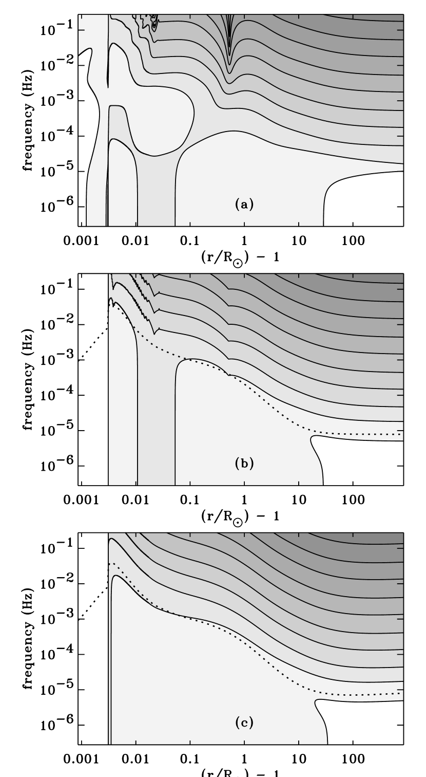
Figure 3.— Contour plot of the reflection coefficient ${\cal R}$ as a function of height and wave frequency. Exact numerical results (a) are compared with results of applying approximations of Sections 2.2–2.4 (b), as well as the more approximate results of estimating critical point conditions using Section 2.5 (c). The 3 panels use identical definitions for the contour levels. From light to dark (i.e., from bottom to top along the right-hand side), the solid contours represent values of ${\cal R}$ of 0.9, 0.3, 0.1, 0.03, 0.01, 0.003, 0.001, $3\times 10^{-4}$, $10^{-4}$, and $3\times 10^{-5}$. Dotted lines in (b) and (c) show the bridging frequency ($\omega_{0}(r)/2\pi$) for the two approximations.

Overall, the similarities between the three panels of Figure 3 appear to outweigh the differences. At large heights ($r\gtrsim 5\,R_{\odot}$) the high-frequency limiting approximations for ${\cal R}$ produce excellent agreement with the numerical solutions. The full radial dependence at very low frequencies ($\omega/2\pi\lesssim 10^{-6}$ Hz) is well reproduced by the results of Section 2.2. There are some discrepancies between the three panels at heights in the low corona (between 0.003 and 0.1 $R_{\odot}$) at low and intermediate frequencies. However, these discrepancies involve mainly the positions of the contours labeling ${\cal R}=0.1$ and 0.3, and the approximations here do not show more than a factor of two difference from the numerical solutions. The effects of $\mu$ changing sign are apparent at heights of about 0.02 and 0.5 $R_{\odot}$ for the highest frequencies, but these “spikes” are smoothed over for frequencies lower than about 0.01 Hz. The average of the two high-frequency approximations (Equation (19)) produces a small cusp at these heights, which is an adequate representation of the mean radial behavior of ${\cal R}$ at these frequencies.

In order to apply the computed reflection coefficients to a model of turbulent dissipation and heating, one needs to understand the properties of the continuous power spectrum $P_{\rm A}(\omega)$ of Alfvénic fluctuation energy in the corona and solar wind. In other words, one needs to know how much is contributed by each frequency (i.e., each “row” in Figure 3) to the total turbulent energy. Although there are observational constraints on the frequency dependence of $P_{\rm A}(\omega)$ at the solar photosphere (Cranmer & van Ballegooijen 2005) and there are direct in situ measurements at distances greater than 60 $R_{\odot}$ (Tu & Marsch 1995; Goldstein et al.  1997), there are no measurements of the Alfvénic frequency spectrum in the extended corona and inner solar wind. Unfortunately, the heights without measured power spectra appear to be the most important for the specification of the rates of heating and momentum deposition in the models.

In this paper, the frequency-weighting of the modeled reflection coefficients will be presented for two empirically based choices for the shape of $P_{\rm A}(\omega)$. Figure 4 displays both spectra, each of which has been normalized such that

$$\int_{0}^{\infty}d\omega\,\,P_{\rm A}(\omega)\,=\,1\,\,.$$ (26)

For simplicity, the normalized spectrum is assumed to retain its shape as a function of height. This assumption has served reasonably well in existing models of solar wind acceleration (e.g., Cranmer et al.  2007), but in reality there must be some kind of spectral evolution with increasing distance from the Sun. A model of this evolution can be straightforwardly combined with the approximations of Section 2, but that is beyond the scope of this paper (see, however, Tu & Marsch 1995; Laitinen 2005; Verdini et al.  2009).

Figure 4.— Normalized Alfvén wave power spectra for the model of Cranmer & van Ballegooijen (2005) (solid curve) and for a Kolmogorov (1941) power law with frequency limits from Verdini & Velli (2007) (dashed curve). Also shown, with arbitrary normalization, is the measured coronal power spectrum from Tomczyk & McIntosh (2009) (dotted curve).

The solid curve in Figure 4 shows the power spectrum of total (kinetic plus magnetic) wave energy from the model of Cranmer & van Ballegooijen (2005) taken at the base of the corona. This model was constrained at the photospheric lower boundary by a measured power spectrum of the kinetic motions of G-band bright points. These bright points represent thin magnetic flux tubes that undergo both random walks, in response to convective granulation, and rapid horizontal “jumps” that appear to be the result of sporadic merging and fragmenting. The spectrum at the coronal base was computed as the result of a non-WKB model of kink-mode and Alfvén-mode transport in the chromosphere and transition region. The dashed curve in Figure 4 shows a power-law spectrum reminiscent of Kolmogorov (1941) hydrodynamic turbulence. The lower and upper limits in frequency were obtained from the non-WKB reflection models of Verdini & Velli (2007), who studied the implications of a $\omega^{-5/3}$ power law spectrum on the coronal heating rate.

For comparison, Figure 4 also shows a measured power spectrum of Alfvénic fluctuations in the low corona (Tomczyk & McIntosh 2009) from a series of Doppler images made by the Coronal Multi-channel Polarimeter (CoMP) at the Sacramento Peak Observatory. It should be noted that the coronal regions that dominated the measured spectrum were closed loops in a coronal active region. Because a turbulent cascade behaves somewhat differently in open and closed regions (e.g., Rappazzo et al.  2008; Cranmer 2009), there may not be a good reason to assume that this spectrum would exist in the source regions of the solar wind. There also may be frequency-dependent line-of-sight integration effects that change the shape of the spectrum. It is nonetheless interesting that this measured spectrum appears to combine the overall power-law behavior of the Kolmogorov (1941) curve with a hint of the high-frequency convective resonance features in the Cranmer & van Ballegooijen (2005) spectrum.

The spectrum-weighted reflection coefficient $\langle{\cal R}\rangle$ is defined as

$$\langle{\cal R}\rangle^{2}(r)\,=\,\frac{\int d\omega\,P_{A}(\omega)\,{\cal R}^{2}(\omega,r)}{\int d\omega\,P_{A}(\omega)}\,\,,$$ (27)

where the square of ${\cal R}$ is used because the power spectrum is an energy density quantity and ${\cal R}$ is a ratio of amplitudes. Equation (27) was used in the solar wind acceleration models of Cranmer et al.  (2007). A slightly different technique was applied by Cranmer & van Ballegooijen (2005), who performed the weighting on the energy densities of the $z_{+}$ and $z_{-}$ fluctuations separately, and then computed their ratio afterwards. The resulting heating rates from the two techniques are not significantly different from one another.

In Figure 5, the radial dependences of the weighted reflection coefficients $\langle{\cal R}\rangle$ are shown for the exact and approximate calculations. Note that ${\cal R}$ (for all frequencies) is set to 1 at heights below the TR. This is obviously not an exact representation of the numerically integrated value, but—as can be seen below in Figure 6—the resulting heating rate is insensitive to these differences.

Figure 5.— Weighted reflection coefficients, shown as a function of radial distance, for (a) the Cranmer & van Ballegooijen (2005) spectrum and (b) the truncated Kolmogorov (1941) spectrum. In each panel, exact numerical results (solid curves) are compared with approximate results computed with known $r_{0}$ and $V_{0}$ (dashed curves) and the approximate results computed with local estimates for $r_{0}$ and $V_{0}$ from Section 2.5 (dotted curves). Measured ranges for fast-wind reflection coefficients from Helios and Ulysses are shown as individual error bars.

Because the Kolmogorov spectrum is dominated by the lowest frequencies, the reflection is dominated by the zero-frequency limit of Section 2.2. Thus, the comparison in Figure 5(b) between the exact result and the approximation computed with known values of $r_{0}$ and $V_{0}$ shows nearly exact agreement. The curves in Figure 5(a) are dominated by higher frequencies and show more of a relative discrepancy between the exact and approximate expressions. For both panels, the reflection coefficients $\langle{\cal R}\rangle$ computed with the estimated values of $r_{0}$ and $V_{0}$ (i.e., the dotted curves) show a significantly more “smoothed out” radial dependence than the other two sets of curves. This gives rise to smoother radial variations in the heating rates. Although this smoothing represents a departure from the exact non-WKB results, it is probably not a major problem. Complete models of coronal heating and solar wind acceleration must also contain heat conduction, and no matter what fine radial structure may exist in the heating rate itself, the existence of conduction gives rise to a similar kind of smearing of the thermal energy along the magnetic field.

Figure 5 also shows Helios and Ulysses measurements in the fast solar wind that have been processed from the Elsässer energy densities presented by Bavassano et al.  (2000). The upper and lower limits of the error bars reflect the spread in individual data points, each of which represented one-hour datasets. The frequency range of the fluctuations sampled by these measurements spanned only about an order of magnitude, from $3\times 10^{-4}$ Hz to $4\times 10^{-3}$ Hz. As can be seen in Figure 4, this range of frequencies is where the two theoretical spectra have comparable power to one another. It is the frequencies outside this narrow range that give rise to the significant differences between the modeled sets of curves in Figures 5(a) and 5(b). Contributions from higher frequencies drive down the reflection coefficient in Figure 5(a), and contributions from lower frequencies drive it up in Figure 5(b). Thus, it is not surprising that the measurements of power at intermediate frequencies give reflection coefficients that fall between the two sets of curves.

3.2. Turbulent Heating Rates

The adopted phenomenological rate of coronal heating is an expression for the total energy flux that cascades from large to small scales. It is constrained by the properties of the fluctuations at the largest scales, and it does not specify the exact kinetic means of dissipation once the energy reaches the smallest scales. Dimensionally, this is similar to the rate of cascading energy flux derived by von Kármán & Howarth (1938) for isotropic hydrodynamic turbulence. The full form, which takes into account various MHD effects, is

$$Q_{\rm turb}\,=\,\rho\,{\cal E}_{\rm turb}\,\frac{Z_{-}^{2}Z_{+}+Z_{+}^{2}Z_{-}}{4L_{\perp}}$$ (28)

(Hossain et al.  1995; Zhou & Matthaeus 1990; Matthaeus et al.  1999; Dmitruk et al.  2001, 2002; Breech et al.  2008). The individual components of Equation (28) are described below.

The absolute values of the spectrum-weighted Elsässer variables are denoted $Z_{+}$ and $Z_{-}$. Strictly speaking, in a model of non-WKB wave reflection the power in both components can be specified only by combining the derived reflection coefficient ${\cal R}$ with a specification of the absolute power spectrum of the fluctuation energy. However, the assumption that the total wave power varies in accord with straightforward wave action conservation has been shown to be reasonable, even in interplanetary space where ${\cal R}$ is not small (Zank et al.  1996; Cranmer & van Ballegooijen 2005). The examples shown below utilize this assumption in order to compute $Z_{+}$ and $Z_{-}$.

Under wave action conservation, the product of a (modified) energy flux and the transverse area of the flux tube remains constant as a function of radial distance. For dispersionless Alfvén waves, this is equivalent to maintaining a constant energy flux per unit magnetic field strength, or

$$\frac{F}{B_{0}}\,=\,\frac{(u+V_{\rm A})^{2}U_{\rm A}}{V_{\rm A}B_{0}}\,=\,\mbox{constant ,}$$ (29)

where the wave energy density $U_{\rm A}=\rho v_{\perp}^{2}$ (see, e.g., Jacques 1977). Measurements of $v_{\perp}$ can be made by analyzing the nonthermal Doppler broadening of coronal emission lines. At $r\approx 1.1\,R_{\odot}$, measurements made by the SUMER instrument on SOHO corresponded to a range of perpendicular velocity amplitudes $v_{\perp}\approx 50$–60 km s^-1 (Banerjee et al.  1998; Landi & Cranmer 2009). Using the plasma parameters from the coronal hole model discussed above, these amplitudes are consistent with a range of values for $F/B_{0}$ between about $5\times 10^{4}$ and $8\times 10^{4}$ erg cm^-2 s^-1 G^-1. At $r\approx 1.5\,R_{\odot}$, lower and upper limit measurements made by the UVCS instrument on SOHO gave a range of amplitudes $v_{\perp}\approx 100$–140 km s^-1 (Esser et al.  1999). These are consistent with a range of $F/B_{0}$ values similar to those at the lower height: $6\times 10^{4}$ to $10^{5}$ erg cm^-2 s^-1 G^-1.

The empirically constrained models of Cranmer & van Ballegooijen (2005) were used as another way to put limits on the most likely wave amplitudes in the corona. These models included wave dissipation due to the presence of turbulence, so the “constant” $F/B_{0}$ actually decreases slightly with increasing distance. In those models, the numerical values of $F/B_{0}$ ranged between about $2\times 10^{4}$ and $9\times 10^{4}$ erg cm^-2 s^-1 G^-1. For the remainder of this paper, an intermediate constant value of $5\times 10^{4}$ erg cm^-2 s^-1 G^-1 is assumed. With that, the full radial dependence of $U_{\rm A}$ can be computed, and the spectrum-averaged Elsässer amplitudes can be determined from

$$Z_{-}\,=\,\sqrt{\frac{4U_{\rm A}}{\rho(1+\langle{\cal R}\rangle^{2})}}\,\,,\,\,\,\,Z_{+}\,=\,\langle{\cal R}\rangle Z_{-}$$ (30)

for use in Equation (28).

The perpendicular length scale $L_{\perp}$ is an effective transverse correlation length of the turbulence for the largest eddies. The models presented here use a standard assumption that the correlation length scales with the transverse width of the magnetic flux tube; i.e., that $L_{\perp}\propto B_{0}^{-1/2}$ (see also Hollweg 1986). Cranmer & van Ballegooijen (2005) found that the following normalization produced a reasonable combination of heating and wave dissipation:

$$L_{\perp}(r)\,\approx\,\frac{11.55}{\sqrt{B_{0}(r)}}\,\,\mbox{Mm ,}$$ (31)

where $B_{0}$ is measured in Gauss. However, the self-consistent models of Cranmer et al.  (2007) worked best by reducing the normalization by about a factor of four; i.e., by replacing the factor of 11.55 in the above by the smaller value 2.876. With no convincing evidence to choose between these two values, the example models shown below use a compromise value of 6.0 Mm for this normalization.

The quantity ${\cal E}_{\rm turb}$ in Equation (28) is an efficiency factor that attempts to account for regions where the turbulent cascade may not have time to develop before the fluctuations are carried away by the wind. Cranmer et al.  (2007) estimated this efficiency factor to scale as

$${\cal E}_{\rm turb}\,=\,\frac{1}{1+(t_{\rm eddy}/t_{\rm ref})^{n}}\,\,,$$ (32)

where the two timescales above are $t_{\rm eddy}$, a nonlinear eddy cascade time, and $t_{\rm ref}$, a timescale for large-scale Alfvén wave reflection. The value $n=1$ was chosen for the exponent based on a range of analytic and numerical turbulence models (Pouquet et al.  1976; Dobrowolny et al.  1980; Matthaeus & Zhou 1989; Dmitruk & Matthaeus 2003; Oughton et al.  2006). Equation (32) quenches the turbulent heating when $t_{\rm eddy}\gg t_{\rm ref}$, i.e., when the Alfvén waves want to propagate away much faster than the cascade can proceed at a given location. Cranmer et al.  (2007) defined the reflection time as $t_{\rm ref}=1/|\nabla\cdot{\bf V}_{A}|$. For the purposes of this paper, the simpler approximation $t_{\rm ref}=\nu^{-1}$ was found to give an equivalent result (see Equation (17)). This latter definition is used in the results presented below. The eddy cascade time is given by

$$t_{\rm eddy}\,=\,\frac{L_{\perp}\sqrt{3\pi}}{(1+M_{A})\,v_{\perp}}\,\,,$$ (33)

where the Alfvén Mach number $M_{A}=u/V_{A}$ and the numerical factor of $3\pi$ comes from the normalization of an assumed shape of the turbulence spectrum (see Appendix C of Cranmer & van Ballegooijen 2005).

Figure 6 shows the computed heating rates for the various spectrum-weighted cases discussed above. Rather than plot $Q_{\rm turb}$ itself, Figure 6 shows the heating rate per unit mass $Q_{\rm turb}/\rho$ in order to more clearly indicate which heights receive the most heating on a particle-by-particle basis. As in Figure 5, the differences between the exact and approximate non-WKB results are relatively minor.

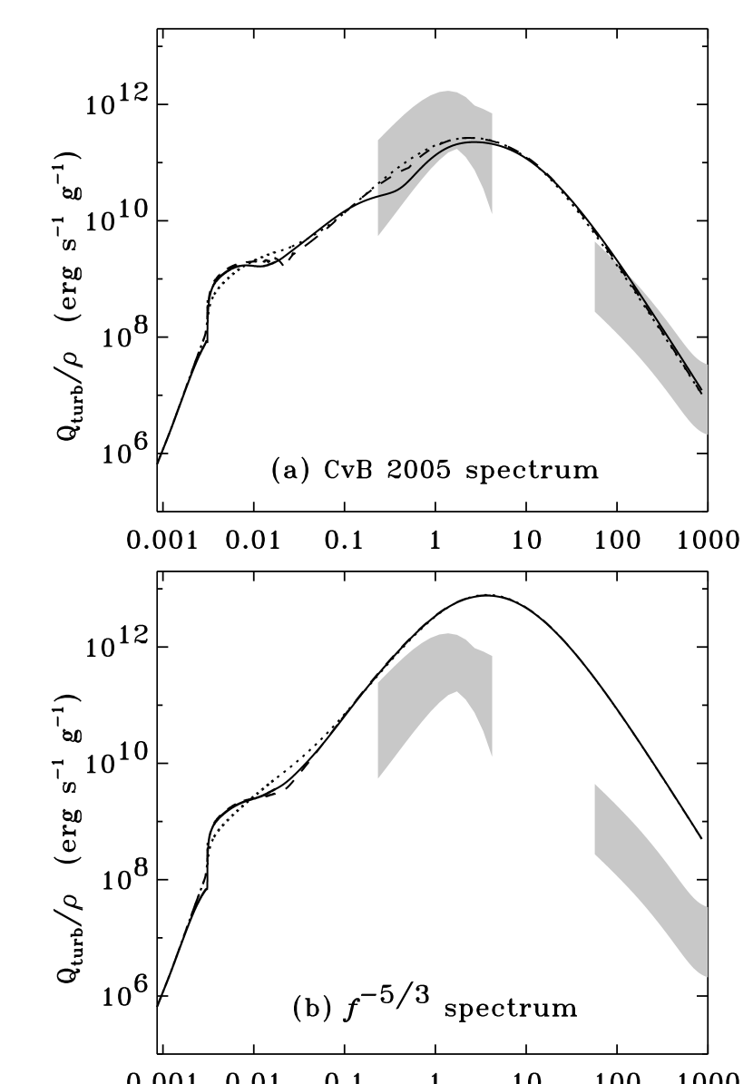
Figure 6.— Turbulent heating rate per unit mass ($Q_{\rm turb}/\rho$) for the coronal hole models. The curves shown in panels (a) and (b), and the line plotting styles in each panel, are the same as in Figure 5. The gray regions show empirically constrained heating rates (see the text).

Each panel of Figure 6 also shows observational constraints on the heating rate in the fast solar wind. The gray region in the corona (i.e., at heights between 0.2 and 6 $R_{\odot}$ above the surface) delineates the lower and upper bounds on a set of parameterized heating rates taken from a range of papers (Wang 1994; Hansteen & Leer 1995; Allen et al.  1998; Cranmer et al.  2007). These are heating rates that are required for these one-dimensional coronal models to be able to produce realistic fast solar wind conditions. Figure 2(b) of Cranmer (2004) illustrates some of the individual heating functions that were collected into this set. The gray region in interplanetary space (i.e., at heights greater than $\sim$60 $R_{\odot}$) illustrates the range of total ($Q_{p}+Q_{e}$) heating rates determined empirically by Cranmer et al.  (2009) from Helios and Ulysses plasma measurements in the fast wind.

Note that the heating rates computed from the high-frequency-dominated spectrum of Cranmer & van Ballegooijen (2005)—shown in Figure 6(a)—tend to be in better agreement with the empirical constraints than do the heating rates computed from the low-frequency-dominated spectrum, in Figure 6(b). This is consistent with the results of Cranmer et al.  (2007), in which a similar high-frequency-dominated spectrum was used to produce reasonably successful models of both fast and slow solar wind streams. Note also that both sets of model results in Figure 6 overestimate the measured heating in interplanetary space. This is likely to be the result of modeling the radial dependence of $Z_{\pm}$ with wave action conservation. In the models of Cranmer & van Ballegooijen (2005), the turbulent dissipation produced a factor of 4 reduction in $v_{\perp}$ at 1 AU, from 144 km s^-1 (undamped) to 35.2 km s^-1 (damped). This would give about a factor of $4^{3/2}=8$ decrease in the heating rate far from the Sun. Inserting this into the present models would push the curves in Figure 6(a) to the bottom of the empirical range, and it would push the curves in Figure 6(b) down to the top of the empirical range.

3.3. Fast and Slow Wind Source Regions

Although the numerical examples shown above were computed for the fast solar wind that emerges from a polar coronal hole, the approximations developed in this paper are not meant to be limited to only that type of solar wind. Figure 7 shows heating rates computed not only for coronal holes, but also source regions of slow wind at solar minimum (i.e., the legs of quiescent equatorial streamers) and at solar maximum (i.e., active regions). These models are self-consistent numerical calculations of the non-WKB reflection, turbulent heating, and wind acceleration that were described by Cranmer et al.  (2007). The quiescent streamer model corresponds to the “last” open field line that originates at a colatitude of 29.7° in the two-dimensional axisymmetric magnetic field model of Banaszkiewicz et al.  (1998). The active region model has an added component to its magnetic field strength that was parameterized by Cranmer et al.  (2007) as having an exponential height dependence of $B_{\rm A}e^{-(r-R_{\odot})/h}$, where $B_{\rm A}=50$ G and $h=0.07\,R_{\odot}$.

Figure 7.— Comparisons of plasma parameters for source regions of fast and slow solar wind: i.e., polar coronal holes (solid curves), quiescent equatorial streamers (dashed curves), and active region field lines connected to the solar wind (dotted curves). Numerical results for (a) outflow velocity, and (b) heating rate per unit mass from Cranmer et al.  (2007) are compared with heating rates computed using the HEATCVB code (c).

Figure 7(a) shows the radial dependence of the wind speed $u$ for these three models. Note that the active region model has an outflow speed of order 100 km s^-1 in the low corona. This appears to correspond with recent measurements of active region outflows of similar magnitude made by the Extreme-ultraviolet Imaging Spectrometer (EIS) on Hinode (see, e.g., Harra et al.  2008). Figure 7(b) presents the heating rates per unit mass ($Q_{\rm turb}/\rho$) that were computed self-consistently in the Cranmer et al.  (2007) models. Figure 7(c) shows the heating rates as computed under the approximations of this paper.

For the active region slow wind model, two curves are shown in Figure 7(c). The lower curve was computed using the standard form for the dimensionless turbulent efficiency factor ${\cal E}_{\rm turb}$ given by Equation (32). The upper curve was computed by not using this efficiency factor (i.e., by assuming ${\cal E}_{\rm turb}=1$). Clearly, the strong peak in the heating rate that is seen in Figure 7(b) is reproduced much more satisfactorily when the efficiency factor is not used. The other two models—for the coronal hole and streamer cases—did not exhibit as strong a relative difference in the heating rate when ${\cal E}_{\rm turb}$ was set to unity. It should be noted that this factor was not used in the earliest published versions of Equation (28) (e.g., Hossain et al.  1995), nor is it used in other more recent studies (e.g., Chandran & Hollweg 2009). Thus, this term should still be viewed as an approximate attempt to take account of “wave escape” effects and not the final word in that story. Future improvements in modeling the turbulence-driven solar wind should involve finding a more robust way of expressing how turbulence is quenched in regions where waves escape more rapidly than they can cascade and dissipate.

4. Numerical Code

A brief FORTRAN 77 subroutine called HEATCVB has been developed to implement the approximations and other expressions given in Sections 2 and 3. The source code is included with this paper as online-only material, and it is also provided, with updates as needed, on the author’s web page. There are only four required inputs to this subroutine: the radial distance $r$, the wind speed $u$, the mass density $\rho$, and the magnetic field strength $|B_{0}|$. The primary output of the subroutine is the heating rate $Q_{\rm turb}$ at the location defined by the input parameters. All quantities are assumed to be in cgs/Gaussian units.

In addition to the four required input parameters, the HEATCVB subroutine has three optional input parameters: the radius of the Alfvén critical point $r_{0}$, the speed at this location (i.e., $V_{0}=u(r_{0})=V_{\rm A}(r_{0})$), and the local Alfvén wave velocity amplitude $v_{\perp}$. If the input values of $r_{0}$ or $V_{0}$ are less than or equal to zero, the code will recompute them using the estimation method described in Section 2.5. If the input value of $v_{\perp}$ is less than or equal to zero, it will be recomputed using wave action conservation (i.e., Equation (29)). This approximation appears to be reasonably valid in the corona (where most of the heating occurs), but it overestimates the Alfvén wave amplitudes in interplanetary space.

Another derived quantity that is computed and output by HEATCVB is the local turbulent dissipation rate of the waves, $\gamma=Q_{\rm turb}/(2U_{\rm A})$. This quantity is specified in units of s^-1 and can be used when solving for departures from wave action conservation. The factor of 2 in the above definition assumes the standard convention that $\gamma$ is the damping rate for the wave amplitude. If instead the damping rate for wave energy is required, $\gamma=Q_{\rm turb}/U_{\rm A}$. Cranmer & van Ballegooijen (2005) showed how this kind of wave dissipation is necessary for agreement between measurements of Alfvén wave amplitudes in the corona and in the heliosphere (see also Roberts 1989; Verdini & Velli 2007).

For simplicity, the HEATCVB code does not utilize the $\mu$ gradients described in Section 2.3. Thus, the bridging between the low-frequency and high-frequency limits for ${\cal R}$ is computed using Equation (25) instead of Equation (19). The weighting of ${\cal R}$ over the Alfvénic power spectrum is performed using the high-frequency-dominated spectrum of Cranmer & van Ballegooijen (2005). As described above, the use of this particular choice of the spectrum worked well for the self-consistent solar wind models of Cranmer et al.  (2007). The integration over the normalized power spectrum is discretized into bins separated by factors of two in frequency space (i.e., “octaves”). The wave power in each bin $i$ is summed into weighting factors $f_{i}$, such that Equation (27) is approximated by

$$\langle{\cal R}\rangle^{2}\,\approx\,\sum_{i}f_{i}\,{\cal R}^{2}(\omega_{i})\,\,.$$ (34)

To make the above compatible with Equation (27), the weights $f_{i}$ are defined such that they sum to 1. The HEATCVB code uses 17 bins that span more than four orders of magnitude in frequency space. The code also contains several checks to ensure that the input parameters are within reasonable bounds for the solar atmosphere and solar wind. All major steps in the algorithm are described in comments within the source code.

The HEATCVB routine contains several tests to evaluate whether a full calculation of the non-WKB reflection is warranted. Whenever $u\leq 0$, the code avoids this calculation and sets $\langle{\cal R}\rangle=1$. The general assumption in this case is that the local plasma is in a closed-field region. The condition $u=0$ could correspond to a hydrostatic coronal streamer, and $u<0$ could signal the existence of transient downflows similar to those observed with visible-light coronagraphs (Wang et al.  1999). In flux tubes where both footpoints are anchored to the solar surface, Alfvén waves are believed to propagate up and down with nearly equal intensities in the two Elsässer components (see, e.g., Rappazzo et al.  2008). Also, whenever $\rho\geq 2\times 10^{-13}$ g cm^-3 the local plasma conditions are judged to be “chromospheric.” In this case, the code sets $\langle{\cal R}\rangle=1$ because it assumes the location to be modeled is below the sharp reflection barrier of the TR. This density criterion may also be triggered for coronal mass ejections (CMEs). These regions may be similar to the above case of coronal loops, since the field lines are closed in CME plasmoids, and the shocked regions in front of the plasmoids are generally believed to have both footpoints rooted to the solar surface (e.g., Lin et al.  2003). However, in CMEs the assumption of time-steady wave action conservation may not give an accurate value for the local fluctuation amplitude $v_{\perp}$.

5. Conclusions

The primary aim of this paper has been to develop and test a set of approximations to the solutions of the equations of non-WKB Alfvén wave reflection. These solutions are designed to be applied to modeling the plasma heating in open-field regions of the solar corona and the solar wind. Two independent approximate expressions for the reflection coefficients ${\cal R}$ were developed in the limiting cases of extremely low wave frequencies (Section 2.2) and extremely high wave frequencies (Section 2.3). These, together with a technique to estimate the radius and speed at the Alfvén critical point, provide a robust approximation for the necessary ingredients of the phenomenological turbulent heating rate. The resulting radial dependence of ${\cal R}$ and the heating rate $Q_{\rm turb}$ were shown to agree well with exact solutions of the non-WKB transport equations in several cases relevant to the fast and slow solar wind.

Because the approximations presented above do not depend on computationally intensive integrations along flux tubes, they make it much easier to insert more realistic (wave/turbulence heating) physics into three-dimensional models of the corona and heliosphere. An important first step is to perform “testbed” simulations for specific time periods in which large amounts of empirical data are available. Such times include the Whole Sun Month in 1996 (Galvin & Kohl 1999) and the Whole Heliosphere Interval in 2008 (Gibson et al.  2009). These testbed models can help determine whether, for example, the WTD or RLO paradigms for solar wind acceleration are better representations of the actual physics (see Section 1). These models will also be key to assessing and validating real-time predictive models of the plasma conditions in the heliosphere.

A significant remaining unknown quantity in the above modeling methodology is the shape of the frequency spectrum of Alfvén waves in the corona. The HEATCVB code utilizes an empirically constrained spectrum from the work of Cranmer & van Ballegooijen (2005). This particular form of the spectrum was shown by Cranmer et al.  (2007) to produce reasonably successful self-consistent models of both fast and slow solar wind streams, so it appears to be a good first approximation. However, this can be replaced easily with other forms of the power spectrum if better constraints become available. It is also likely that the shape of the power spectrum depends on radial distance and cannot be specified universally for all values of $r$ (e.g., Verdini et al.  2009). Once such a radial dependence is specified, however, the approximations developed in this paper can still be used to estimate the turbulent heating at any location along the open field lines.

In order to make further progress, it will be important to include other physical processes in WTD-type models of coronal heating and solar wind acceleration. In addition to non-WKB reflection, there are other ways that the energy in outward propagating waves can be tapped to produce inward propagating waves. Large-scale shear motions in the heliosphere have been suggested as a source of kinetic energy that could go into reducing the overall cross helicity of the turbulence (e.g., Roberts et al.  1992; Zank et al.  1996; Matthaeus et al.  2004; Breech et al.  2008; Usmanov et al.  2009). Kinetic instabilities in collisionless regions of the corona and solar wind can give rise to the local generation of high-frequency inward propagating waves (Isenberg 2001; Isenberg et al.  2009). Also, outward propagating Alfvén waves of sufficient amplitude may become unstable to nonlinear processes—such as “parametric decay”—which give rise to enhanced inward propagating wave activity (e.g., Goldstein 1978; Jayanti & Hollweg 1993; Lau & Siregar 1996; Ofman & Davila 1998; Suzuki & Inutsuka 2006; Hollweg & Isenberg 2007).

Although the phenomenological heating rate given in Equation (28) was motivated by the results of many analytic and numerical studies, there is still some disagreement about its robustness and applicability. Chandran et al.  (2009) found that the exact dependence of the dissipation rate on $Z_{+}$ and $Z_{-}$ may depend on the specific generation mechanism(s) of inward propagating waves. Also, the evolution of the correlation length $L_{\perp}$ with radial distance should be coupled to the overall evolution of $Z_{\pm}$ and not simply scaled with the flux-tube width as in Equation (31) (see, e.g., Matthaeus et al.  1999; Breech et al.  2009).

Finally, it will be important for future models to take account of the multi-fluid nature of coronal heating and solar wind acceleration. A large-scale description of the energy flux injected into the turbulent cascade is needed in order to model its eventual kinetic dissipation (and the subsequent preferential energization of electrons, protons, and heavy ions). Even in the strongly collisional “low corona,” there are likely to be macroscopic dynamical consequences of the partitioning of energy between protons and electrons (see, e.g., Hansteen & Leer 1995; Endeve et al.  2004). Non-WKB Alfvén wave reflection also affects the energy and momentum coupling between protons and other ions in the solar wind (Li & Li 2007, 2008). Including these effects can lead to concrete predictions for measurements to be made by space missions such as Solar Probe (McComas et al.  2007) and Solar Orbiter (Marsden & Fleck 2007), as well as next-generation ultraviolet coronagraph spectroscopy that could follow up on the successes of the UVCS instrument on SOHO (Kohl et al.  2006).

References

- (1) Allen, L. A., Habbal, S. R., & Hu, Y. Q. 1998, J. Geophys. Res., 103, 6551
- (2) An, C.-H., Suess, S. T., Moore, R. L., & Musielak, Z. E. 1990, ApJ, 350, 309
- (3) Axford, W. I., & McKenzie, J. F. 1992, in Solar Wind Seven, ed. E. Marsch & R. Schwenn (New York: Pergamon), 1
- (4) Banaszkiewicz, M., Axford, W. I., & McKenzie, J. F. 1998, A&A, 337, 940
- (5) Banerjee, D., Teriaca, L., Doyle, J. G., & Wilhelm, K. 1998, A&A, 339, 208
- (6) Barkhudarov, M. R. 1991, Sol. Phys., 135, 131
- (7) Bavassano, B., Pietropaolo, E., & Bruno, R. 2000, J. Geophys. Res., 105, 15959
- (8) Breech, B., Goldstein, M. L., Roberts, D. A., & Usmanov, A. V. 2009, in AIP Conf. Proc., Solar Wind 12 (Melville, NY: AIP), in press
- (9) Breech, B., Matthaeus, W. H., Minnie, J., Oughton, S., Parhi, S., Bieber, J. W., & Bavassano, B. 2005, Geophys. Res. Lett., 32, L06103
- (10) Breech, B., Matthaeus, W. H., Minnie, J., Bieber, J. W., Oughton, S., Smith, C. W., & Isenberg, P. A. 2008, J. Geophys. Res., 113, A08105
- (11) Chandran, B. D. G., & Hollweg, J. V. 2009, ApJ, 707, 1659
- (12) Chandran, B. D. G., Quataert, E., Howes, G. G., Hollweg, J. V., & Dorland, W. 2009, ApJ, 701, 652
- (13) Cranmer, S. R. 2004, in SOHO-15: Coronal Heating, ed. R. W. Walsh, J. Ireland, D. Danesy, & B. Fleck (Noordwijk, The Netherlands: ESA), ESA SP-575, 154
- (14) Cranmer, S. R. 2009, Living Rev. Solar Phys., 6, lrsp-2009-3
- (15) Cranmer, S. R., Matthaeus, W. H., Breech, B. A., & Kasper, J. C. 2009, ApJ, 702, 1604
- (16) Cranmer, S. R., & van Ballegooijen, A. A. 2005, ApJS, 156, 265
- (17) Cranmer, S. R., van Ballegooijen, A. A., & Edgar, R. J. 2007, ApJS, 171, 520
- (18) Dmitruk, P., & Matthaeus, W. H. 2003, ApJ, 597, 1097
- (19) Dmitruk, P., Matthaeus, W. H., Milano, L. J., Oughton, S., Zank, G. P., & Mullan, D. J. 2002, ApJ, 575, 571
- (20) Dmitruk, P., Milano, L. J., & Matthaeus, W. H. 2001, ApJ, 548, 482
- (21) Dobrowolny, M., Mangeney, A., & Veltri, P. 1980, Phys. Rev. Lett., 45, 144
- (22) Eastwood, J. P. 2008, Phil. Trans. Roy. Soc. A, 366, 4489
- (23) Elsässer, W. M. 1950, Phys. Rev., 79, 183
- (24) Endeve, E., Holzer, T. E., & Leer, E. 2004, ApJ, 603, 307
- (25) Esser, R., Fineschi, S., Dobrzycka, D., Habbal, S. R., Edgar, R. J., Raymond, J. C., Kohl, J. L., & Guhathakurta, M. 1999, ApJ, 510, L63
- (26) Evans, R. M., Opher, M., Manchester, W. B., IV, & Gombosi, T. I. 2008, ApJ, 687, 1355
- (27) Feng, X., Zhou, Y., & Wu, S. T. 2007, ApJ, 655, 1110
- (28) Ferraro, C. A., & Plumpton, C. 1958, ApJ, 127, 459
- (29) Feynman, J., & Gabriel, S. B. 2000, J. Geophys. Res., 105, 10543
- (30) Fisk, L. A., Schwadron, N. A., & Zurbuchen, T. H. 1999, J. Geophys. Res., 104, 19765
- (31) Galvin, A. B., & Kohl, J. L. 1999, J. Geophys. Res., 104, 9673
- (32) Gibson, S. E., Kozyra, J. U., de Toma, G., Emery, B. A., Onsager, T., & Thompson, B. J. 2009, J. Geophys. Res., 114, A09105
- (33) Goldstein, M. L. 1978, ApJ, 219, 700
- (34) Goldstein, M. L., Roberts, D. A., & Matthaeus, W. H. 1997, in Cosmic Winds and the Heliosphere, ed. J. R. Jokipii, C. P. Sonett, & M. S. Giampapa (Tucson: U. Arizona Press), 521
- (35) Hansteen, V. H., & Leer, E. 1995, J. Geophys. Res., 100, 21577
- (36) Harra, L. K., Sakao, T., Mandrini, C. H., Hara, H., Imada, S., Young, P. R., van Driel-Gesztelyi, L., & Baker, D. 2008, ApJ, 676, L147
- (37) Heinemann, M., & Olbert, S. 1980, J. Geophys. Res., 85, 1311
- (38) Hollweg, J. V. 1978, Sol. Phys., 56, 305
- (39) Hollweg, J. V. 1981, Sol. Phys., 70, 25
- (40) Hollweg, J. V. 1986, J. Geophys. Res., 91, 4111
- (41) Hollweg, J. V. 1990, J. Geophys. Res., 95, 14873
- (42) Hollweg, J. V., & Isenberg, P. A. 2007, J. Geophys. Res., 112, A08102
- (43) Hossain, M., Gray, P. C., Pontius, D. H., Jr., Matthaeus, W. H., & Oughton, S. 1995, Phys. Fluids, 7, 2886
- (44) Isenberg, P. A. 2001, J. Geophys. Res., 106, 29249
- (45) Isenberg, P. A., Vasquez, B. j., Chandran, B. D. G., & Pongkitiwanichakul, P. 2009, in AIP Conf. Proc., Solar Wind 12 (Melville, NY: AIP), in press
- (46) Jacques, S. A. 1977, ApJ, 215, 942
- (47) Jayanti, V., & Hollweg, J. V. 1993, J. Geophys. Res., 98, 19049
- (48) Kohl, J. L., Noci, G., Cranmer, S. R., & Raymond, J. C. 2006, A&A Rev., 13, 31
- (49) Kolmogorov, A. N. 1941, Dokl. Akad. Nauk SSSR, 30, 301
- (50) Krogulec, M., Musielak, Z. E., Suess, S. T., Nerney, S. F., & Moore, R. L. 1994, J. Geophys. Res., 99, 23489
- (51) Laitinen, T. 2005, Astrophys. Space Sci. Trans., 1, 35
- (52) Landi, E., & Cranmer, S. R. 2009, ApJ, 691, 794
- (53) Lau, Y.-T., & Siregar, E. 1996, ApJ, 465, 451
- (54) Li, B., & Li, X. 2007, ApJ, 661, 1222
- (55) Li, B., & Li, X. 2008, ApJ, 682, 667
- (56) Lin, J., Soon, W., & Baliunas, S. L. 2003, New Astron. Reviews, 47, 53
- (57) Lionello, R., Linker, J. A., & Mikić, Z. 2009, ApJ, 690, 902
- (58) MacGregor, K. B., & Charbonneau, P. 1994, ApJ, 430, 387
- (59) Marsden, R. G., & Fleck, B. 2007, in ASP Conf. Ser. 368, The Physics of Chromospheric Plasmas, ed. P. Heinzel, I. Dorotovič, & R. Rutten (San Francisco: ASP), 645
- (60) Matthaeus, W. H., Minnie, J., Breech, B., Parhi, S., Bieber, J. W., & Oughton, S. 2004, Geophys. Res. Lett., 31, L12803
- (61) Matthaeus, W. H., Zank, G. P., Oughton, S., Mullan, D. J., & Dmitruk, P. 1999, ApJ, 523, L93
- (62) Matthaeus, W. H., & Zhou, Y. 1989, Phys. Fluids B, 1, 1929
- (63) McComas, D. J., et al. 2007, Rev. Geophys., 45, RG1004
- (64) Musielak, Z. E., Moore, R. L., Suess, S. T., & An, C.-H. 1989, ApJ, 344, 478
- (65) Nakamizo, A., Tanaka, T., Kubo, Y., Kamei, S., Shimazu, H., & Shinagawa, H. 2009, J. Geophys. Res., 114, A07109
- (66) Ofman, L., & Davila, J. M. 1998, J. Geophys. Res., 103, 23677
- (67) Orlando, S., Lou, Y.-Q., Rosner, R., & Peres, G. 1996, J. Geophys. Res., 101, 24433
- (68) Oughton, S., Dmitruk, P., & Matthaeus, W. H. 2006, Phys. Plasmas, 13, 042306
- (69) Parker, E. N. 1958, ApJ, 128, 664
- (70) Pouquet, A., Frisch, U., & Leorat, J. 1976, J. Fluid Mech., 77, 321
- (71) Press, W. H., Teukolsky, S. A., Vetterling, W. T., & Flannery, B. P. 1992, Numerical Recipes in Fortran: The Art of Scientific Computing (Cambridge: Cambridge Univ. Press)
- (72) Rappazzo, A. F., Velli, M., Einaudi, G., & Dahlburg, R. B. 2007, ApJ, 657, L47
- (73) Rappazzo, A. F., Velli, M., Einaudi, G., & Dahlburg, R. B. 2008, ApJ, 677, 1348
- (74) Riley, P., Linker, J. A., & Mikić, Z. 2001, J. Geophys. Res., 106, 15889
- (75) Riley, P., Linker, J. A., Mikić, Z., Lionello, R., Ledvina, S. A., & Luhmann, J. G. 2006, ApJ, 653, 1510
- (76) Roberts, D. A. 1989, J. Geophys. Res., 94, 6899
- (77) Roberts, D. A., Goldstein, M. L., Matthaeus, W. H., & Ghosh, S. 1992, J. Geophys. Res., 97, 17115
- (78) Roussev, I. I., Gombosi, T. I., Sokolov, I. V., Velli, M., Manchester, W., IV, DeZeeuw, D. L., Liewer, P., Tóth, G., & Luhmann, J. 2003, ApJ, 595, L57
- (79) Schmit, D. J., Gibson, S., de Toma, G., Wiltberger, M., Hughes, W. J., Spence, H., Riley, P., Linker, J. A., & Mikić, Z. 2009, J. Geophys. Res., 114, A06101
- (80) Schwadron, N. A., & McComas, D. J. 2003, ApJ, 599, 1395
- (81) Sokolov, I. V., Roussev, I. I., Skender, M., Gombosi, T. I., & Usmanov, A. V. 2009, ApJ, 696, 261
- (82) Suzuki, T. K., & Inutsuka, S.-I. 2006, J. Geophys. Res., 111, A06101
- (83) Tomczyk, S., & McIntosh, S. W. 2009, ApJ, 697, 1384
- (84) Tóth, G., et al. 2005, J. Geophys. Res., 110, A12226
- (85) Tu, C.-Y., & Marsch, E. 1995, Space Sci. Rev., 73, 1
- (86) Usmanov, A. V., & Goldstein, M. L. 2006, J. Geophys. Res., 111, A07101
- (87) Usmanov, A. V., Matthaeus, W. H., Breech, B., & Goldstein, M. L. 2009, in ASP Conf. Ser. 406, Numerical Modeling of Space Plasma Flows, ed. N. Pogorelov, E. Audit, P. Colella, & G. Zank (San Francisco: ASP), 160
- (88) Vásquez, A. M., van Ballegooijen, A. A., & Raymond, J. C. 2003, ApJ, 598, 1361
- (89) Velli, M. 1993, A&A, 270, 304
- (90) Verdini, A., & Velli, M. 2007, ApJ, 662, 669
- (91) Verdini, A., Velli, M., & Buchlin, E. 2009, ApJ, 700, L39
- (92) Verdini, A., Velli, M., & Oughton, S. 2005, A&A, 444, 233
- (93) von Kármán, T., & Howarth, L. 1938, Proc. Roy. Soc. London A, 164, 192
- (94) Wang, Y.-M. 1994, ApJ, 435, L153
- (95) Wang, Y.-M., & Sheeley, N. R., Jr. 1991, ApJ, 372, L45
- (96) Wang, Y.-M., Sheeley, N. R., Jr., Howard, R. A., St. Cyr, O. C., & Simnett, G. M. 1999, Geophys. Res. Lett., 26, 1203
- (97) Wentzel, D. G. 1978, Sol. Phys., 58, 307
- (98) Zank, G. P., Matthaeus, W. H., & Smith, C. W. 1996, J. Geophys. Res., 101, 17093
- (99) Zhou, Y., & Matthaeus, W. H. 1990, J. Geophys. Res., 95, 10291