Sensitivity of the limit shape of sample clouds from meta densities

Abstract

The paper focuses on a class of light-tailed multivariate probability distributions. These are obtained via a transformation of the margins from a heavy-tailed original distribution. This class was introduced in Balkema et al. (J. Multivariate Anal. 101 (2010) 1738–1754). As shown there, for the light-tailed meta distribution the sample clouds, properly scaled, converge onto a deterministic set. The shape of the limit set gives a good description of the relation between extreme observations in different directions. This paper investigates how sensitive the limit shape is to changes in the underlying heavy-tailed distribution. Copulas fit in well with multivariate extremes. By Galambos’s theorem, existence of directional derivatives in the upper endpoint of the copula is necessary and sufficient for convergence of the multivariate extremes provided the marginal maxima converge. The copula of the max-stable limit distribution does not depend on the margins. So margins seem to play a subsidiary role in multivariate extremes. The theory and examples presented in this paper cast a different light on the significance of margins. For light-tailed meta distributions, the asymptotic behaviour is very sensitive to perturbations of the underlying heavy-tailed original distribution, it may change drastically even when the asymptotic behaviour of the heavy-tailed density is not affected.

, and

1 Introduction

In recent years, meta distributions have been used in several applications of multivariate probability theory, especially in finance. The construction of meta distributions can be illustrated by a simple example. Start with a multivariate spherical Student $t$ distribution and transform its margins to be Gaussian. We call the new distribution a meta distribution with normal margins based on the original $t$ distribution. Since the copula of a multivariate distribution is invariant under strictly increasing coordinatewise transformations, the original distribution and the meta distribution share their copula and hence have the same dependence structure. Random vectors with Gaussian densities have asymptotically independent components, whatever the correlation. In contrast, the above meta distribution with Gaussian margins inherits not only the dependence properties of the original $t$ distribution, but also the asymptotic dependency. Asymptotic dependence is of importance in risk analysis. It yields rank-based measures of tail dependence, and coefficients of tail dependence (see, e.g., Chapter 5 in [4]).

Our interest is in extremes. The asymptotic behaviour of sample clouds gives a very intuitive view of multivariate extremes. Sample clouds from light-tailed densities tend to have a well-defined shape. The limit shape, if it exists, describes the relation between extreme observations in different directions; it indicates in which directions more severe extremes are likely to occur, and how much more extreme these will be. It has been shown in [2] that sample clouds from meta distributions in the standard set-up, see below, can be scaled to converge onto a limit set. The boundary of this limit set has a simple explicit analytic description. Surprisingly, the limit shape of sample clouds from the meta distribution contains no information about the shape of the sample clouds from the original distribution. The results of the present paper further support this point.

Multivariate distribution functions (d.f.s) have the property that there is a simple relation between the d.f. of the underlying random vector and the d.f. of the coordinatewise maximum of any number of independent observations from this distribution. One just raises the d.f. to the given power. This makes d.f.s ideal tools to handle coordinatewise maxima, and to study their limit behaviour. This rather analytic approach sometimes obscures the probabilistic content of the results. The approach via densities and probability measures on ${\mathbb{R}}^{d}$ which is taken in this paper may at first seem clumsy, but it has the advantage that there is a close relation to what one observes in the sample clouds.

The aim of the paper is to investigate stability of the shape of the limit set under changes in the original distribution. We look at changes which do not affect the margins, or at least their asymptotic behaviour. Keeping margins (asymptotically) unchanged allows us to isolate the role played by the copula. We shall examine how much the original and meta distributions in the standard set-up may be altered without affecting the asymptotic behaviour of the scaled sample clouds. This indicates how robust the limit shape is. Then we move on to explore sensitivity. It turns out that the limit shape of the scaled sample clouds from the light-tailed meta distribution is very sensitive to certain slight perturbations of the original distribution. Sensitivity depends on the region.

Our results suggest that the recipe outlined above for constructing multivariate distributions with Gaussian margins with the copula of a heavy-tailed density with a pronounced dependence structure in the limit has to be treated with caution. The limit shape of the sample clouds from the meta distribution is affected by perturbations of the original heavy-tailed density, perturbations which are so small that they do not influence the multivariate extreme value behaviour. In going from densities with heavy-tailed margins to the meta densities with light-tailed margins, the dependence structure of the max-stable limit distribution is preserved by a well-known invariance result in multivariate extreme value theory (EVT). In this paper we shall give conditions on the severity of changes in the original heavy-tailed distribution which are allowed if one wants to retain the asymptotic behaviour of the coordinatewise extremes, and show that perturbations which are negligible compared to these changes may affect the limit shape of the sample clouds of the associated light-tailed meta distribution.

The present paper is a follow-up to [2]. The latter paper contains a detailed analysis of meta densities and gives the motivation and implications of the assumptions in the standard set-up. It presents the derivation of the analytic form in (8) of the limit shape of the sample clouds from the light-tailed meta distribution. In the present paper, Section 2 introduces the notation and recalls the relevant definitions and results from [2]. Section 3 is the heart of the paper; here we present details of the constructions which demonstrate robustness and sensitivity of the limit shape of sample clouds from meta distributions. Concluding remarks are given in Section 4.

Summary of notation

Several of the basic symbols used in the paper are summarized in Table 1.

Table 1: Miscellaneous symbols

Symbol	Description
$f\asymp\tilde{f}$	weak asymptotic equality: ratios $f({\mathbf{x}})/\tilde{f}({\mathbf{x}})$ and $\tilde{f}({\mathbf{x}})/f({\mathbf{x}})$ are bounded eventually
	for $\|{\mathbf{x}}\|\to\infty$
$f\sim\tilde{f}$	asymptotic equality: $\tilde{f}({\mathbf{x}})/f({\mathbf{x}})\to 1$ for $\|{\mathbf{x}}\|\to\infty$
$n_{D}$	the gauge function of the set $D$: $n_{D}({\mathbf{x}})>0$ for ${\mathbf{x}}\neq{\mathbf{0}}$, $D=\{n_{D}<1\}$ and
	$n_{D}(c{\mathbf{x}})=cn_{D}({\mathbf{x}})$ for ${\mathbf{x}}\in{\mathbb{R}}^{d}$, $c\geq 0$
${\mathbf{e}}$; $E_{\times}$	a vector of ones in ${\mathbb{R}}^{d}$; the diagonal cross (see (10))
$B$, $C$	the open Euclidean unit ball in ${\mathbb{R}}^{d}$; the open cube $(-1,1)^{d}$

Throughout the paper, it is convenient to keep in mind two spaces: ${\mathbf{z}}$-space on which the heavy-tailed d.f.s $F,F^{*},\ldots$ are defined, and ${\mathbf{x}}$-space on which the light-tailed meta d.f.s $G,G^{*},\ldots$ are defined. Table 2 compares notation used for mathematical objects on these two spaces.

Table 2: Symbols used to distinguish various objects of interest in ${\mathbf{z}}$-space and in ${\mathbf{x}}$-space. Notation for margins assumes that all marginal densities are equal and symmetric

${\mathbf{z}}$-space	${\mathbf{x}}$-space	Comments
$F$ and $f$	$G=F\circ K$ and $g$	joint d.f. and density
$F_{0}$ and $f_{0}$	$G_{0}=F_{0}\circ K_{0}$ and $g_{0}$	margin d.f. and density
$\pi$	$\mu$	probability measures
$\pi_{n}$	$\mu_{n}$	mean measures of scaled sample clouds
${\mathbf{Z}}$, ${\mathbf{Z}}_{1},{\mathbf{Z}}_{2},\ldots$	${\mathbf{X}}$, ${\mathbf{X}}_{1},{\mathbf{X}}_{2},\ldots$	random vectors
$N_{n}$	$M_{n}$	scaled $n$-point sample clouds
$N$: Poisson point process	$E$: limit set	limit of scaled sample clouds
$c_{n}\colon\ 1-F_{0}(c_{n})\sim 1/n$	$b_{n}\colon\ -\log(1-G_{0}(b_{n}))\sim\log n$	scaling constants
$(B_{n})$, $t_{n}=K_{0}(s_{n})$	$(A_{n})$, $s_{n}$	block partitions, division points

2 Preliminaries

2.1 Definitions and standard set-up

Meta distributions are constructed by transforming margins of a given multivariate distribution so as to obtain a new (meta) distribution with desired margins. To fix our notation and terminology, let us present this construction procedure formally.

Consider a random vector ${\mathbf{Z}}$ in ${\mathbb{R}}^{d}$ with d.f. $F$ and continuous margins $F_{i}$, $i=1,\ldots,d$. Let $G_{1},\ldots,G_{d}$ be continuous d.f.s on ${\mathbb{R}}$ which are strictly increasing on the intervals $I_{i}=\{0<G_{i}<1\}$. Define the transformation

$$K(x_{1},\ldots,x_{d})=(K_{1}(x_{1}),\ldots,K_{d}(x_{d})),\qquad K_{i}(s)=F_{i}^{-1}(G_{i}(s)),\qquad i=1,\ldots,d.$$ (1)

The d.f. $G=F\circ K$ is called the meta distribution with margins $G_{i}$ based on the original d.f. $F$. The coordinatewise map $K=K_{1}\otimes\cdots\otimes K_{d}$, which maps ${\mathbf{x}}=(x_{1},\ldots,x_{d})\in I=I_{1}\times\cdots\times I_{d}$ into the vector ${\mathbf{z}}=(K_{1}(x_{1}),\ldots,K_{d}(x_{d}))$, is called the meta transformation.

In the paper, we restrict attention to meta distributions with light-tailed margins based on a heavy-tailed original distribution. The precise assumptions we make on the meta margins and the original distribution are summarized in the standard set-up given in Definition 2 below. But before stating assumptions of the standard set-up, we need several additional definitions and notation.

Recall the basic example we started with in the introduction of a meta distribution with normal margins based on a multivariate $t$ distribution. The multivariate $t$ density has a simple structure. It is fully characterized by the shape of its level sets, scaled copies of the defining ellipsoid, and by the decay $c/r^{\lambda+d}$ of its tails along rays. The constant $\lambda>0$ denotes the degrees of freedom, $d$ the dimension of the underlying space, and $c$ is a positive constant depending on the direction of the ray. In the more general setting of the paper, the tails of the density are allowed to decrease as $cL(r)/r^{\lambda+d}$ for some slowly varying function $L$ and the condition of elliptical level sets is replaced by the requirement that the level sets are equal to scaled copies of a fixed bounded convex or star-shaped set (a set $D$ is star-shaped if ${\mathbf{z}}\in D$ implies $t{\mathbf{z}}\in D$ for $0\leq t<1$). Due to the power decay of the tails, the density $f$ is said to be heavy-tailed. Densities with the above properties constitute the class ${\mathcal{F}}_{\lambda}$.

Definition 1.

The set ${\mathcal{F}}_{\lambda}$ for $\lambda>0$ consists of all positive continuous densities $f$ on ${\mathbb{R}}^{d}$ which are asymptotic to a function of the form $f_{*}(n_{D}({\mathbf{z}}))$, where $f_{*}(r)=L(r)/r^{(\lambda+d)}$ is a continuous decreasing function on $[0,\infty)$, $L$ varies slowly, and $n_{D}$ is the gauge function of the set $D$ (see Table 1). The set $D$ is bounded, open and star-shaped. It contains the origin and the gauge function is continuous.

The reader may keep in mind the case where $D$ is a convex symmetric set, $D=-D$. In that case, the gauge function is a norm, and $D$ the open unit ball in this norm. In the standard set-up, the normal margins of the meta density in the introduction are generalized to include densities whose tails are asymptotic to a von Mises function: $g_{0}(s)\sim\mathrm{e}^{-\psi(s)}$ for $s\to\infty$ with scale function $a=1/\psi^{\prime}$, where $\psi$ is a $C^{2}$ function with a positive derivative such that

$$\psi(s)\to\infty,\qquad a(s)^{\prime}\to 0,\qquad s\to\infty.$$ (2)

This condition on the meta margins ensures that they lie in the maximum domain of attraction of the Gumbel limit law $\exp(-\mathrm{e}^{-x})$, $x\in{\mathbb{R}}$; see, for example, Proposition 1.4 in [5].

We are now able to define the standard set-up.

Definition 2.

Let $f$ be a density in ${\mathcal{F}}_{\lambda}$ for some $\lambda>0$ with margins all equal to a positive continuous symmetric density $f_{0}$, and let $g_{0}$ be a continuous, positive, symmetric density on ${\mathbb{R}}$ asymptotic to a von Mises function $\mathrm{e}^{-\psi}$, where in addition to (2) $\psi$ is assumed to vary regularly at infinity with exponent $\theta>0$. In the standard set-up, the meta density $g$ is based on $f$ and has margins $g_{0}$.

This set-up is the same as in [2] except that for simplicity we additionally assume that the original density has equal margins. As a consequence, the components of the meta transformation $K$ are equal:

$$K\mathchoice{\nobreak\,\colon}{\nobreak\,\colon}{\nobreak\,\colon\;}{\nobreak\,\colon\;}{\mathbf{x}}\mapsto{\mathbf{z}}=(K_{0}(x_{1}),\ldots,K_{0}(x_{d})),\qquad K_{0}=F_{0}^{-1}\circ G_{0},\qquad K_{0}(-t)=-K_{0}(t).$$ (3)

2.2 Convergence of sample clouds

An $n$-point sample cloud is the point process consisting of the first $n$ points of a sequence of independent observations from a given distribution, after proper scaling. We write

$$N_{n}=\{{\mathbf{Z}}_{1}/a_{n},\ldots,{\mathbf{Z}}_{n}/a_{n}\},$$ (4)

where ${\mathbf{Z}}_{1},{\mathbf{Z}}_{2},\ldots$ are independent observations from the given probability distribution on ${\mathbb{R}}^{d}$, and $a_{n}$ are positive scaling constants. It is customary to write $N_{n}(A)$ for the number of the points of the sample cloud that fall into the set $A$.

In this section, we discuss the asymptotic behaviour of sample clouds from the original density $f$ and from the associated meta density $g$ in the standard set-up. The difference in the asymptotic behaviour is striking: sample clouds from the heavy-tailed density $f$ converge in distribution to a Poisson point process on ${\mathbb{R}}^{d}\setminus\{{\mathbf{0}}\}$ whereas sample clouds from the light-tailed meta density $g$ tend to have a clearly defined boundary. They converge onto a deterministic set.

2.2.1 Convergence for densities in ${\mathcal{F}}_{\lambda}$ and measures in ${\mathcal{D}}_{\lambda}$

For densities in ${\mathcal{F}}_{\lambda}$, $\lambda>0$, there is a simple limit relation which follows from the regular variation of the function $f_{*}$ in Definition 1 and from the homogeneity of the gauge function:

$${\displaystyle\frac{f(r_{n}{\mathbf{w}}_{n})}{f_{*}(r_{n})}}\to h({\mathbf{w}}),\qquad{\mathbf{w}}_{n}\to{\mathbf{w}}\neq{\mathbf{0}},r_{n}\to\infty,$$ (5)

where

$$h({\mathbf{w}})=1/n_{D}({\mathbf{w}})^{\lambda+d}.$$ (6)

Convergence is uniform and ${\mathbf{L}}^{1}$ on the complement of centered balls. If ${\mathbf{Z}}_{1},{\mathbf{Z}}_{2},\ldots$ are independent observations from the density $f$ then the sample clouds $N_{n}$ in (4) converge in distribution to the Poisson point process with intensity $h$ weakly on the complement of centered balls for a suitable choice of scaling constants $a_{n}$.

A probability measure $\pi$ on ${\mathbb{R}}^{d}$ varies regularly with scaling function $a(t)\to\infty$ if there is an infinite Radon measure $\rho$ on ${\mathbb{R}}^{d}\setminus\{{\mathbf{0}}\}$ such that the finite measures $t\pi$ scaled by $a(t)$ converge to $\rho$ vaguely on ${\mathbb{R}}^{d}\setminus\{{\mathbf{0}}\}$. The measure $\rho$ has the scaling property

$$\rho(rA)=\rho(A)/r^{\lambda},\qquad r>0$$ (7)

for all Borel sets $A$ in ${\mathbb{R}}^{d}\setminus\{{\mathbf{0}}\}$. The constant $\lambda\geq 0$ is the exponent of regular variation. If it is positive, then $\rho$ gives finite mass to the complement of the open unit ball $B$ and weak convergence holds on the complement of centered balls. We shall denote the set of all probability measures which vary regularly with exponent $\lambda>0$ and with limit measure $\rho$ by ${\mathcal{D}}_{\lambda}(\rho)$ (or just ${\mathcal{D}}_{\lambda}$). In particular, $\pi\in{\mathcal{D}}_{\lambda}$ if $\pi$ has a continuous density in ${\mathcal{F}}_{\lambda}$. As above, for independent observations ${\mathbf{Z}}_{1},{\mathbf{Z}}_{2},\ldots$ from a distribution $\pi\in{\mathcal{D}}_{\lambda}(\rho)$ the scaled sample clouds $N_{n}$ in (4) (with scaling constants $a_{n}$) converge in distribution to a Poisson point process with mean measure $\rho$ weakly on the complement of centered balls (since the mean measures converge; see, e.g., Proposition 3.21 in [5] or Theorem 11.2.V in [3]).

2.2.2 Convergence for meta densities in the standard set-up

Sample clouds from light-tailed meta densities in the standard set-up, under suitable scaling, converge onto a deterministic set, referred to as the limit set, in the sense of the following definition.

Definition 3.

For a compact set $E$ in ${\mathbb{R}}^{d}$, the $n$-point point processes $N_{n}$ converge onto $E$ as $n\to\infty$ if for open sets $U$ containing $E$, the probability of a point outside $U$ vanishes, ${\mathbb{P}}\{N_{n}(U^{c})>0\}\to 0$, and if

$${\mathbb{P}}\{N_{n}({\mathbf{p}}+\e B)>m\}\to 1\qquad\mbox{for all $m\geq 1$ and $\e>0$, ${\mathbf{p}}\in E$.}$$

We now recall Theorem 2.6 of [2], which characterizes the shape of the limit set for meta distributions in the standard set-up.

Theorem 2.1.

Let the meta density $g$ satisfy the assumptions of the standard set-up of Definition 2. Define

$$E:=E_{\lambda,\theta}=\{{\mathbf{u}}\in{\mathbb{R}}^{d}\mid|u_{1}|^{\theta}+\cdots+|u_{d}|^{\theta}+\lambda\geq(\lambda+d)\|{\mathbf{u}}\|_{\infty}^{\theta}\}.$$ (8)

If $\psi(r_{n})\sim\log n$, then for the sequence of independent observations ${\mathbf{X}}_{1},{\mathbf{X}}_{2},\ldots$ from the meta density $g$ the sample clouds $M_{n}=\{{\mathbf{X}}_{1}/r_{n},\ldots,{\mathbf{X}}_{n}/r_{n}\}$ converge onto $E$.

Figure 1 illustrates the limit set $E_{\lambda,\theta}$ in the above theorem for several values of the parameters $\lambda$ and $\theta$. The sample cloud in Panel (a) of the figure is simulated from the meta distribution with standard Gaussian margins based on a Cauchy distribution with elliptic level sets. Hence, the associated limit set has parameters $\lambda=1$ and $\theta=2$.

(a)	(b)

Figure 1: Panel (a): A sample cloud of 10,000 points from a meta distribution with standard Gaussian margins based on a Cauchy distribution. Panel (b): The limit sets $E_{\lambda,\theta}$ in (8) with $\theta=2$ and $\lambda=1,2,4,10$ (solid, dash, dot, dotdash lines, resp.).

2.3 Further notation and conventions

In order to ease the exposition, we introduce some additional assumptions and notation.

All univariate d.f.s are assumed to be continuous and strictly increasing. The d.f.s $F_{0}$ and $\tilde{F}_{0}$ on ${\mathbb{R}}$ are tail asymptotic if

$$\tilde{F}_{0}(-t)/F_{0}(-t)\to 1,\qquad\bigl{(}1-\tilde{F}_{0}(t)\bigr{)}/\bigl{(}1-F_{0}(t)\bigr{)}\to 1,\qquad t\to\infty.$$

The sample clouds from a heavy-tailed d.f. $\tilde{F}$ converge to the point process $\tilde{N}$ if $\tilde{N}$ is a Poisson point process on ${\mathbb{R}}^{d}\setminus\{{\mathbf{0}}\}$, and if the sample clouds converge to $\tilde{N}$ in distribution weakly on the complement of centered balls, where the scaling constants $c_{n}$ satisfy $1-\tilde{F}_{0}(c_{n})\sim 1/n$. Two heavy-tailed d.f.s $F^{*}$ and $F^{**}$ have the same asymptotics if the margins are tail asymptotic and if the sample clouds converge to the same point process. The light-tailed d.f.s $G^{*}$ and $G^{**}$ have the same asymptotics if the margins are tail asymptotic and the sample clouds converge onto the same compact set $E^{*}$, with scale factors $b_{n}$ which satisfy $-\log(1-G_{0}(b_{n}))\sim\log n$. One may replace a scaling sequence by a sequence asymptotic to it without affecting the limit. The scaling of sample clouds is determined up to asymptotic equality by the margins since the univariate projections have to converge. Tail asymptotic margins yield asymptotic scalings.

3 Results

3.1 Preview

We now turn our attention to the main issue of the paper. We start out with a pair of d.f.s $F$ and $G=F\circ K$ which satisfy the conditions of the standard set-up. Introduce a new pair $(F^{*},G^{*})$ where $F^{*}$ and $G^{*}=F^{*}\circ K$ are related by the same meta transformation $K$, and where one term of the pair has the same asymptotic behaviour as the corresponding term in $(F,G)$. What does this imply for the other term of the pair?

1. [(Q.2)]

2. If the scaled sample clouds from $G^{*}$ and from $G$ converge onto the same set $E$, do the scaled sample clouds from $F^{*}$ converge to the same point process $N$ as those from $F$?

3. If the scaled sample clouds from $F^{*}$ and from $F$ converge to the same Poisson point process $N$, do the scaled sample clouds from $G^{*}$ converge onto the same set $E$ as those from $G$?

For coordinatewise maxima, convergence is determined by the copula and the answer to the questions is “Yes.” If the margins lie in the univariate domain of attraction and $F$ and $G$ have the same copula then convergence of the coordinatewise maxima and the associated sample clouds for one d.f. implies convergence for the other d.f. In the situation of this paper the answer to both questions is “No.” For example, for (Q.1), if we replace $f$ by a weakly asymptotic density $f^{*}\asymp f$, the asymptotic behaviour of sample clouds from $g^{*}$ is not affected, since $g^{*}\asymp g$ (see Lemma 3.2 below), but the scaled sample clouds from $f^{*}$ obviously need not converge. This section contains some counterexamples which will be worked out further in the next two sections.

What we want to do is specify the margins $f_{0}$ and $g_{0}$ (which determine the meta transformation $K$), then vary the copula and check the limit behaviour of the sample clouds (where we impose the condition that both converge). We are looking for d.f.s $F^{*}$ and $G^{*}$ with the properties:

1. [(P.3)]

2. $F^{*}$ has marginal densities $f_{0}$;

3. $G^{*}$ is the meta distribution based on $F^{*}$ with marginal densities $g_{0}$;

4. the scaled sample clouds from $F^{*}$ converge to a Poisson point process $N^{*}$;

5. the scaled sample clouds from $G^{*}$ converge onto a compact set $E^{*}$.

Moreover, we would like $E^{*}$ to be the set $E_{\lambda,\theta}$ in (8), or $N^{*}$ to have mean measure $\rho^{*}=\rho$ with intensity $h$ in (6). So we either choose $F^{*}$ to have the same asymptotics as $F$, or $G^{*}$ to have the same asymptotics as $G$. Note that the conditions (P1)–(P4) have certain implications. The mean measure $\rho^{*}$ of the Poisson point process $N^{*}$ is an excess measure with exponent $\lambda$, see (7), its margins are equal and symmetric with intensity $\lambda/|t|^{\lambda+1}$ since the marginal densities $f_{0}$ are equal and symmetric and the scaling constants $c_{n}$ ensure that $\rho\{w_{d}\geq 1\}=1$. The limit set $E^{*}$ is a subset of the cube $C=[-1,1]^{d}$ and projects onto the interval $[-1,1]$ in each coordinate, again by our choice of the scaling constants.

The two sections below describe procedures for altering distributions without changing the margins too much. The first procedure uses block partitions. A block partition is a special kind of partition into coordinate blocks. If the blocks are relatively small, then the asymptotics of a distribution do not change if one replaces it by one which gives the same mass to each block. Block partitions are mapped into block partitions by the meta transformation $K$. The mass is preserved, but the size and shape of the blocks may change drastically. The block partitions provide insight in the relation between the asymptotic behaviour of the measures $\mathrm{d}F^{*}$ and $\mathrm{d}G^{*}$. In the second procedure, we replace $\mathrm{d}F$ by a probability measure $\mathrm{d}\tilde{F}$, which agrees outside a bounded set with a mixture $\mathrm{d}(F+F^{o})$, where $F^{o}$ has lighter margins than $F$:

$$F_{j}^{o}(-t)\ll F_{0}(-t),\qquad 1-F_{j}^{o}(t)\ll 1-F_{0}(t),\qquad t\to\infty,\ j=1,\ldots,d.$$ (9)

This condition ensures that $\tilde{F}$ and $F$ have the same asymptotics. The two corresponding light-tailed meta d.f.s $\tilde{G}$ and $G$ on ${\mathbf{x}}$-space may have different asymptotics since the scaling constants $b^{o}_{n}$ and $b_{n}$ may be asymptotic even though $G^{o}$ has lighter tails than $G$. If this is the case, and the scaled sample clouds from $G^{o}$ converge onto a compact set $E^{o}$, then those from $\tilde{G}$ converge onto the union $E\cup E^{o}$, which may be larger than $E$. These two procedures enable us to construct d.f.s $F^{*}$ and $G^{*}=F^{*}\circ K$ with the same marginal densities as the d.f.s $F$ and $G$ in the standard set-up which exhibit unexpected behaviour:

1. [(Ex.2)]

2. $G^{*}$ and $G$ have the same asymptotics, but the scaled sample clouds from $F^{*}$ converge to a Poisson point process which lives on the diagonal. (See Proposition 3.7 and Example 1.)

3. The scaled sample clouds from $G^{*}$ converge onto $E^{*}=A\cup E_{\times}$, where $E_{\times}$ is the diagonal cross

   $$E_{\times}=\{r\delta\mid 0\leq r\leq 1,\delta\in\{-1,1\}^{d}\},$$ (10)

   and $A$ is the closure of an open star-shaped set $D\subset(-1,1)^{d}$ with a continuous gauge function $n_{D}$, see Table 1 above. The d.f.s $F^{*}$ and $F$ have the same asymptotics. The density $f^{*}$ is asymptotic to $f$ on every ray. (See Proposition 3.9 and Example 1.)

What does the copula say about the asymptotics? Everything, since it determines the d.f. if the margins are given; nothing, since the examples above show that there is no relation between the asymptotics of $F^{*}$ and the asymptotics of $G^{*}$ even with the prescribed margins $f_{0}$ and $g_{0}$. One might hope that at least the parameters $\lambda$ and $\theta$, determined by the margins, might be preserved in the asymptotics. The point process $N^{*}$ reflects the parameter $\lambda$ in the marginal intensities $\lambda/|t|^{\lambda+1}$. However, $E^{*}=E_{\lambda^{*},\theta^{*}}$ may hold for any $\lambda^{*}$ and $\theta^{*}$ in $(0,\infty)$ by taking $A=E_{\lambda^{*},\theta^{*}}$ in (Ex.2) above.

We now start with the technical details.

The construction procedures discussed above will change an original d.f. $\hat{F}$ with margins $F_{0}$ into a d.f. $\tilde{F}$ whose margins $\tilde{F}_{j}$ are tail equivalent to $F_{0}$. This is no serious obstacle.

Proposition 3.1.

Let the scaled sample clouds from $\tilde{F}$ converge to a point process $\tilde{N}$, and let the scaled sample clouds from $\tilde{G}=\tilde{F}\circ K$ converge onto the compact set $\tilde{E}$. If the margins $\tilde{F}_{j}$ are continuous and strictly increasing and tail asymptotic to $F_{0}$, then there exists a d.f. $F^{*}$ with margins $F_{0}$ such that $F^{*}$ has the same asymptotics as $\tilde{F}$ and $G^{*}=F^{*}\circ K$ has the same asymptotics as $\tilde{G}$.

If moreover $\tilde{F}$ has a density $\tilde{f}$ with margins asymptotic to $f_{0}$ at $\pm\infty$, then $F^{*}$ has a density $f^{*}$, and for any vector ${\mathbf{w}}$ with nonzero coordinates and any sequence ${\mathbf{w}}_{n}\to{\mathbf{w}}$ and $r_{n}\to\infty$ there is a sequence ${\mathbf{w}}^{\prime}_{n}\to{\mathbf{w}}$ such that $f^{*}(r_{n}{\mathbf{w}}_{n})\sim\tilde{f}(r_{n}{\mathbf{w}}^{\prime}_{n})$.

Proof.

Let $F^{*}=\tilde{F}\circ K_{F}$ be the meta d.f. based on $\tilde{F}$ with margins $F_{0}$. The components $K_{Fj}=\tilde{F}_{j}^{-1}\circ F_{0}$ are homeomorphisms and satisfy $K_{Fj}(t)\sim t$ for $|t|\to\infty$. (Here, we use that the marginal tails vary regularly with exponent $-\lambda\neq 0$.) It follows that

$$\|K_{F}({\mathbf{z}})-{\mathbf{z}}\|/\|{\mathbf{z}}\|\to 0,\qquad\|{\mathbf{z}}\|\to\infty.$$ (11)

This ensures that $\tilde{F}$ and $F^{*}$ have the same asymptotics. (For any $\e>0$, the distance between the scaled sample point ${\mathbf{Z}}/c_{n}$ and $K_{F}({\mathbf{Z}})/c_{n}$ is bounded by $\e\|{\mathbf{Z}}\|/c_{n}$ for $\|{\mathbf{Z}}\|\geq\e c_{n}$ and $n\geq n_{\e}$.) A similar argument shows that $\tilde{G}=\tilde{F}\circ K$ and $G^{*}=F^{*}\circ K$, the meta d.f. based on $\tilde{G}$ with margins $G_{0}$, have the same asymptotics. Here, we use that $\tilde{G}_{j}=\tilde{F}_{j}\circ K_{0}$ is tail asymptotic to $G_{0}=F_{0}\circ K_{0}$ since $\tilde{F}_{j}$ is tail asymptotic to $F_{0}$. Under the assumptions on the density the Jacobian of $K_{F}$ is asymptotic to one in the points $r_{n}{\mathbf{w}}^{\prime}_{n}$ and (11) gives the limit relation with $r_{n}{\mathbf{w}}^{\prime}_{n}=K_{F}^{-1}(r_{n}{\mathbf{w}}_{n})$. ∎

In general, the densities $f^{*}$ and $\tilde{f}$ (in the notation of the above proposition) are only weakly asymptotic, as in Proposition 1.8 in [2]. The density $f^{*}$ on ${\mathbf{z}}$-space is related to $f$ in the same way as the density $g^{*}$ is related to $g$. If $f^{*}\asymp f$ or $f^{*}\leq Cf$ or $f^{*}\sim f$, then these relations also holds for $g^{*}$ and $g$, and vice versa. Similarly, for the margins: $g^{*}_{j}\sim g_{0}$ at $\infty$ implies $f^{*}_{j}\sim f_{0}$ at $\infty$. These results are formalized in the lemma below.

Lemma 3.2.

If $F^{*}$ has density $f^{*}$ with margins $f_{j}^{*}$ and $G^{*}=F^{*}\circ K$ has density $g^{*}$ with margins $g^{*}_{j}$, then

$$g^{*}({\mathbf{x}})/g({\mathbf{x}})=f^{*}({\mathbf{z}})/f({\mathbf{z}}),\qquad g^{*}_{j}(s)/g_{0}(s)=f^{*}_{j}(t)/f_{0}(t),\qquad{\mathbf{z}}=K({\mathbf{x}}),\qquad t=K_{0}(s).$$

Proof.

The Jacobian drops out in the quotients. ∎

3.2 Block partitions

Block partitions are a good tool for testing the robustness and sensitivity of asymptotic behaviour of sample clouds via simple constructions.

Consider a partition of ${\mathbb{R}}^{d}$ into bounded Borel sets $A_{n}$ given by coordinate blocks. Since our d.f.s have continuous margins, the boundaries of the blocks are null sets, and we shall not bother about boundary points, and treat the blocks as open sets. To construct such a block partition start with an increasing sequence of cubes

$$s_{n}C=(-s_{n},s_{n})^{d},\qquad 0<s_{1}<s_{2}<\cdots,s_{n}\to\infty.$$

Subdivide the ring $R_{n}=s_{n+1}C\setminus s_{n}C$ between two successive cubes into blocks by a symmetric partition of the interval $[-s_{n+1},s_{n+1}]$ with division points $\pm s_{nj}$, $j=1,\ldots,m_{n}$ with $s_{nm_{n}}=s_{n}$, $s_{nm_{n}+1}=s_{n+1}$ and

$$-s_{n+1}<-s_{n}<\cdots<-s_{n1}<s_{n1}<\cdots<s_{n}<s_{n+1}.$$

This gives a partition of the cube $s_{n+1}C$ into $(2m_{n}+1)^{d}$ blocks of which $(2m_{n}-1)^{d}$ form the cube $s_{n}C$. The remaining blocks form the ring $R_{n}$. The meta transformation $K$ transforms block partitions in ${\mathbf{x}}$-space into block partitions in ${\mathbf{z}}$-space. A comparison of the original block partition with its transform gives a good indication of the way in which the meta transformation distorts space.

The block partition introduced above is regular if $s_{n+1}\sim s_{n}$ and $\Delta_{n}/s_{n}\to 0$, where $\Delta_{n}$ is the maximum of $s_{n1},s_{n2}-s_{n1},\ldots,s_{nm_{n}}-s_{nm_{n}-1}$.

Our first aim is to investigate how much the d.f.s $F$ and $G=F\circ K$ in the standard set-up may be altered without affecting the asymptotic behaviour of the scaled sample clouds. Regular partitions give a simple answer to a related question: If one replaces density $f$ or $g$ by a discrete distribution, how far apart are the atoms allowed to be if one wants to retain the asymptotic behaviour of the sample clouds from the given density?

Proposition 3.3.

Let $A_{1},A_{2},\ldots$ in ${\mathbf{x}}$-space be a regular block partition. Suppose the sample clouds from the probability distribution $\mu$ scaled by $r_{n}$ converge onto the compact set $E$. Let $\tilde{\mu}$ be a probability measure such that $\tilde{\mu}(A_{n})=\mu(A_{n})$ for $n\geq n_{0}$. Then the sample clouds from $\tilde{\mu}$ scaled by $r_{n}$ converge onto $E$.

Proof.

Let ${\mathbf{p}}\in E$, and $\e>0$. Let $\mu_{n}$ denote the mean measure from the scaled sample cloud from $\mu$ and $\tilde{\mu}_{n}$ the same for $\tilde{\mu}$. Then $\mu_{n}({\mathbf{p}}+(\e/2)B)\to\infty$. Because the sets $A_{n}$ are relatively small there exists $n_{1}$ such that any set $A_{n}$ which intersects the ball $r_{n}{\mathbf{p}}+r_{n}\e B$ with $n\geq n_{1}$ has diameter less than $\e r_{n}/2$. Let $U_{n}$ be the union of the sets $A_{n}$ which intersect $r_{n}{\mathbf{p}}+(r_{n}\e/2)B$. Then $U_{n}\subset r_{n}{\mathbf{p}}+\e r_{n}B$ and hence

$$\mu_{n}\bigl{(}{\mathbf{p}}+(\e/2)B\bigr{)}\leq\mu_{n}(U_{n}/r_{n})=\tilde{\mu}_{n}(U_{n}/r_{n})\leq\tilde{\mu}_{n}({\mathbf{p}}+\e B).$$

Similarly, $\tilde{\mu}_{n}(U^{c})\to 0$ for any open set $U$ which contains $E$. ∎

Remark 1.

The result also holds if $\tilde{\mu}(A_{n})\sim\mu(A_{n})$ provided $\mu(A_{n})$ is positive eventually.

There is an analogous result for regular partitions in ${\mathbf{z}}$-space.

Proposition 3.4.

Suppose $\pi\in{\mathcal{D}}_{\lambda}(\rho)$ with scaling constants $c_{n}$. Let $A_{1},A_{2},\ldots$ be a regular block partition and let $\tilde{\pi}$ be a probability measure on ${\mathbb{R}}^{d}$ such that $\tilde{\pi}(A_{n})=\pi(A_{n})$ for $n\geq n_{0}$. Then $\tilde{\pi}\in{\mathcal{D}}_{\lambda}(\rho)$ with scaling constants $c_{n}$.

Proof.

Any closed block $A\subset{\mathbb{R}}^{d}\setminus\{{\mathbf{0}}\}$ whose boundary carries no $\rho$-mass is contained in an open block $U$ with $\rho(U)<\rho(A)+\e$. As in the proof of the previous proposition, for $n\geq n_{1}$ there is a union $U_{n}$ of atoms $A_{n}$ such that $A\subset U_{n}/c_{n}\subset U$. By homogeneity of $\rho$, the boundary of a block has positive mass $\rho({\rm Phys.~{}Rev.~{}Lett.}B_{n})>0$ only if one of the vertices lies in a coordinate plane. By assumption, the division points are nonzero. ∎

We thus have the following simple situation: $A_{1},A_{2},\ldots$ is a block partition in ${\mathbf{x}}$-space and $B_{1}=K(A_{1}),B_{2}=K(A_{2}),\ldots$ the corresponding block partition in ${\mathbf{z}}$-space, where $K$ is the meta transformation in (3). Let $\tilde{\pi}$ be a probability measure in ${\mathbf{z}}$-space and $\tilde{\mu}$ a probability measure in ${\mathbf{x}}$-space, linked by $K$, that is, $\tilde{\pi}=K(\tilde{\mu})$. Then $\tilde{\pi}(A_{n})=\tilde{\mu}(B_{n})$ for all $n$. So

$$\tilde{\pi}(A_{n})\sim\int_{A_{n}}f({\mathbf{z}})\,\mathrm{d}{\mathbf{z}}\quad\iff\quad\tilde{\mu}(B_{n})\sim\int_{B_{n}}g({\mathbf{x}})\,\mathrm{d}{\mathbf{x}}.$$ (12)

Theorem 3.5.

Assume the standard set-up in Definition 2. If the two block partitions $A_{n}$ and $B_{n}=K(A_{n})$ both are regular, and one of the equivalent asymptotic equalities in (12) holds, then the sample clouds from $\tilde{\pi}$ scaled by $c_{n}$ converge to the Poisson point process with intensity $h$ in (6), and the sample clouds from $\tilde{\mu}$ scaled by $r_{n}$ converge onto the set $E=E_{\lambda,\theta}$ in (8).

Proof.

Combine Propositions 3.3 and 3.4. ∎

Unfortunately, the meta transformation $K$ is very nonlinear. Regularity of one block partition does not imply regularity of the other block partition.

We first consider the case when the block partition $(A_{n})$ in ${\mathbf{x}}$-space is regular, but $(B_{n})$ is not. The block partition $(A_{n})$ in ${\mathbf{x}}$-space is based on a sequence of cubes $s_{n}C=(-s_{n},s_{n})^{d}$. Successive cubes are of the same size asymptotically, $s_{n+1}\sim s_{n}$. The cubes $t_{n}C$ in ${\mathbf{z}}$-space with $t_{n}=K_{0}(s_{n})$ may grow very fast. It is possible that $t_{n}\ll t_{n+1}$. The corresponding partition with blocks $B_{n}=K(A_{n})$ in ${\mathbf{z}}$-space then certainly is not regular.

Proposition 3.6.

Assume the standard set-up. Let $\eta\in(0,1)$. There is a sequence $0<s_{1}<s_{2}<\cdots$ such that $s_{n}\to\infty$ and $s_{n+1}\sim s_{n}$, and such that

$$t_{n}=K_{0}(s_{n})=n^{n^{n^{\eta}}}.$$

Proof.

We have $g_{0}\sim\mathrm{e}^{-\psi}$. This implies $1-G_{0}(s)\sim a(s)g_{0}(s)\sim\mathrm{e}^{-\Psi(s)}$, where $\Psi$ like $\psi$ varies regularly with exponent $\theta$. Write $s_{n}=\mathrm{e}^{\sigma_{n}}$ and $\tau\Psi(s_{n})\sim\mathrm{e}^{\theta r(\sigma_{n})}$, where $r$ is a $C^{2}$ function with $r^{\prime}(t)\to 1$ and $r^{\prime\prime}(t)\to 0$ as $t\to\infty$, and $\tau:=1/\lambda$. It has been shown in [2] (Equation (1.13)) that

$$K_{0}(s)=t\sim c\mathrm{e}^{\varphi(s)},\qquad\varphi(s)=\tau q(\Psi(s))\sim\tau\Psi(s),\qquad s\to\infty$$

for some positive constant $c$. This gives $\log t_{n}=\log K_{0}(s_{n})\sim\mathrm{e}^{\theta r(\sigma_{n})}$. Since $\log\log t_{n}=n^{1-\e}\log n+\log\log n$ has increments which go to zero, so does $\theta r(\sigma_{n})$, and hence also $\sigma_{n}$ since $r^{\prime}$ tends to one. It follows that $s_{n+1}\sim s_{n}$. ∎

Choose $s_{nm_{n}-1}=s_{n-1}$. Then the cube $(s_{n-1}{\mathbf{e}},s_{n+1}{\mathbf{e}})$ is a union of $2^{d}$ blocks in the partition on ${\mathbf{x}}$-space, and so is the cube $(t_{n-1}{\mathbf{e}},t_{n+1}{\mathbf{e}})$ in ${\mathbf{z}}$-space; ${\mathbf{e}}=(1,\ldots,1)$ denotes a vector of ones in ${\mathbb{R}}^{d}$. The union $U$ of these latter cubes has the property that the scaled sets $U/t_{n}$ converge to $(0,\infty)^{d}$ for $t_{n}\to\infty$ if $t_{n}\ll t_{n+1}$.

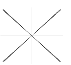
(a)	(b)

Figure 2: Panel (a): Schematic representation of the four sets $U_{\Delta}=\bigcup_{n}[\Delta_{1}t_{n-1}{\mathbf{e}},\Delta_{2}t_{n+1}{\mathbf{e}}]$ in ${\mathbb{R}}^{2}$ for $\Delta=(\Delta_{1},\Delta_{2})\in\{-1,1\}^{2}$; see Proposition 3.7. Panel (b): the image of the sets $U_{\Delta}$ in ${\mathbf{x}}$-space. The division points of the partitions $(A_{n})$ and $(B_{n})$ are $s_{n}=n^{\sqrt{n}}\log n$ and $t_{n}=\mathrm{e}^{s_{n}}=n^{n^{\sqrt{n}}}$, respectively. Use Proposition 3.6 with $K_{0}(s)=\mathrm{e}^{s}$, $s>s_{0}$ and $\e=0.5$. (a) z-space. (b) x-space (regular).

Proposition 3.7.

Assume the standard set-up. The excess measure $\rho$ has the continuous density $h$ in (2.6) and does not charge the coordinate planes. Moreover, $\rho\{\delta z_{i}\geq t\}=1/t^{\lambda}$ for $\delta=\pm 1$, $i=1,\ldots,d$ and $t>0$. Let $\tilde{\rho}$ be an excess measure on ${\mathbb{R}}^{d}\setminus\{{\mathbf{0}}\}$. Assume that for each open orthant $Q_{\Delta}$, $\Delta\in\{-1,1\}^{d}$, the restrictions of $\tilde{\rho}$ and $\rho$ to $Q_{\Delta}$ have the same univariate margins. One may then choose $\tilde{F}$ such that its margins are tail asymptotic to $F_{0}$, such that the sample clouds from $\tilde{F}$ converge to the Poisson point process $\tilde{N}$ with mean measure $\tilde{\rho}$, and such that the sample clouds from the d.f. $\tilde{G}=\tilde{F}\circ K$ converge onto the limit set $E_{\lambda,\theta}$ in (8).

Proof.

We sketch the construction. Choose $\hat{F}\in{\mathcal{D}}_{\lambda}(\tilde{\rho})$ with density $\hat{f}$ such that the sample clouds from $\hat{F}$ scaled by $c_{n}$ converge to $\tilde{N}$. For $\Delta\in\{-1,1\}^{d}$, let $U_{\Delta}$ be the image of the union $U$ in $Q_{\Delta}$ by reflecting coordinates for which $\Delta_{j}=-1$ (see Figure 2 for an illustration). Let $\tilde{f}$ agree with $\hat{f}$ on the $2^{d}$ sets $U_{\Delta}$ and with $f$ elsewhere, so that, by the remark above on the convergence of the scaled sets $U$, $\tilde{f}$ and $\hat{f}$ differ only on an asymptotically negligible set. Alter $\tilde{f}$ on a bounded set to make it a probability density. Then the sample clouds from $\tilde{F}$ scaled by $c_{n}$ converge to $\tilde{N}$. In the corresponding partition $(A_{n})$ on ${\mathbf{x}}$-space we only change the measure on the “tiny” blocks $(s_{n-1},s_{n+1})^{d}$ (with $s_{n-1}\sim s_{n+1}$) around the positive diagonal, and their reflections. Hence, the scaled sample clouds from $\tilde{G}=\tilde{F}\circ K$ converge onto $E_{\lambda,\theta}$. ∎

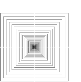
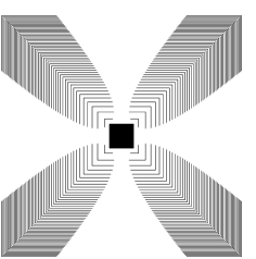
(a)	(b)

Figure 3: Panel (a): blocks $[-t_{n},t_{n}]^{2}=[-\mathrm{e}^{\sqrt{n}},\mathrm{e}^{\sqrt{n}}]^{2}$, $n\in\{2,4,6,\ldots,100\}$ in ${\mathbf{z}}$-space with the sets $[-\mathrm{e}^{\sqrt{n}}/n,\mathrm{e}^{\sqrt{n}}/n]\times[\mathrm{e}^{\sqrt{n-1}},\mathrm{e}^{\sqrt{n}}]$ and their reflections, which correspond to the blocks of partition $(B_{n})$ intersecting the axes, deleted. Panel (b): image of the blocks ($[-\sqrt{n},\sqrt{n}]^{2}$) and deleted blocks ($[-\sqrt{n}+\log n,\sqrt{n}-\log n]\times[\sqrt{n-1},\sqrt{n}]$) from Panel (b) in ${\mathbf{x}}$-space under the meta transformation $K_{0}(s)=\mathrm{e}^{s}$, $s>s_{0}$. (a) z-space (regular). (b) x-space.

We now discuss the second case: the block partition $(B_{n})$ in ${\mathbf{z}}$-space is regular, but $(A_{n})$ is not. Figure 3 depicts sequences of cubes $s_{n}C$ and $t_{n}C$ in ${\mathbb{R}}^{2}$ on which partitions $(A_{n})$ and $(B_{n})$ are based in the special case when $s_{n}=\sqrt{n}$ and $t_{n}=K_{0}(s_{n})=\mathrm{e}^{s_{n}}=\mathrm{e}^{\sqrt{n}}$, along with subintervals $[-\mathrm{e}^{\sqrt{n}}/n,\mathrm{e}^{\sqrt{n}}/n]\times\{\mathrm{e}^{n}\}$ in ${\mathbf{z}}$-space mapping onto $[-\sqrt{n}+\log n,\sqrt{n}-\log n]\times\{\sqrt{n}\}$ in ${\mathbf{x}}$-space, which correspond to the partition blocks intersecting the coordinate axes. We now have the following result.

In the standard set-up with d.f.s $F$ and $G=F\circ K$, margins $F_{0}$ and $G_{0}=F_{0}\circ K_{0}$ and densities $f$ and $g$ there are two formulations of the asymptotic behaviour, analytic and probabilistic. The analytic formulation states that $f(r{\mathbf{w}})/f(r{\mathbf{e}})$ converges for $r\to\infty$ to a limit function $h$ of the form $c/n_{D}^{\lambda+d}$ where $n_{D}$ is a continuous gauge function (of a bounded open star-shaped set $D$ containing the origin). The behaviour of the meta density is quite different: $g(r{\mathbf{u}})/g(r{\mathbf{e}})$ converges to zero on the complement of the compact set $E=E_{\lambda,\theta}$ and tends to $+\infty$ on the interior of this set. The probabilistic version treats the asymptotic behaviour of sample clouds. The sample clouds from $F$, scaled by $a_{n}$, converge to a Poisson point process with intensity $c_{0}h$; the sample clouds from $G$ scaled by $b_{n}$ converge onto $E$. Here

$$1-F_{0}(c_{n})=1-G_{0}(b_{n})=1/n,\qquad c_{n}=K_{0}(b_{n}).$$ (13)

The figures show that the meta transformation $K$ moves points outside the coordinate planes towards the diagonals. The block partitions introduced above enable us to make this more precise.

Proposition 3.8.

Let $F$ and $G=F\circ K$ satisfy the standard set-up with densities $f$ and $g$. There exists a perturbation $\tilde{F}$ with density $\tilde{f}$ and meta d.f. $\tilde{G}=\tilde{F}\circ K$ with density $\tilde{g}$ with the properties:

• $\tilde{f}\leq f$ outside the unit ball, and hence $\tilde{g}\leq g$ outside a bounded set;

• $\tilde{f}\equiv f$ on the $d$ coordinate planes, and hence $\tilde{g}\equiv g$ on the coordinate planes;

• for any unit vector $\zeta$ with nonzero components and any sequences ${\mathbf{z}}_{n}=r_{n}\zeta_{n}$ with $r_{n}\to\infty$ and $\zeta_{n}\to\zeta$ eventually $\tilde{f}({\mathbf{z}}_{n})\equiv f({\mathbf{z}}_{n})$;

• for any unit vector $\xi$ with non-zero components which does not lie on one of the $2^{d}$ diagonal rays and any sequence ${\mathbf{x}}_{n}=r_{n}\xi_{n}$ with $r_{n}\to\infty$ and $\xi_{n}\to\xi$ eventually $\tilde{g}({\mathbf{x}}_{n})=0$;

• the sample clouds from $\tilde{F}$ scaled by $c_{n}$ in (13) converge to a Poisson point process with intensity $c_{0}h$;

• the sample clouds from $\tilde{G}$ scaled by $b_{n}$ in (13) converge onto the diagonal cross $E_{\times}$ in (10).

Proof.

The construction is simple. We introduce a regular partition for $F$, and delete the mass in the atoms $B_{n}$ which intersect a coordinate plane $\{z_{i}=0\}$, replacing it on a thin ridge around the coordinate planes to ensure that the second condition holds. In the end, we increase the density on the unit ball outside the coordinate planes to ensure that the new function $\tilde{f}$ is a probability density. We shall now give the details for dimension $d=2$. We focus on the positive horizontal axis. Choose $t_{n}=n$. Choose $t_{n1}=r_{n}=\mathrm{o}(n)$ but so that $s_{n1}\sim s_{n}=K_{0}^{-1}(t_{n})$. This is possible since slow variation of $L_{0}=K_{0}^{-1}$ implies that $L_{0}(\e t_{n})/L_{0}(t_{n})\to 1$ for any $\e>0$. Set $\tilde{f}\equiv 0$ on the atom $(n-1,n)\times(-r_{n},r_{n})$ but keep $\tilde{f}\equiv f$ on the rectangle $(n-1,n)\times(-\mathrm{e}^{-n},\mathrm{e}^{-n})$. Do this for $n\geq n_{0}$, and do the same for the three other halfaxes. The first four conditions hold by construction. The fifth condition follows by the ${\mathbf{L}}^{1}$ convergence of $\tilde{h}_{n}({\mathbf{w}})=\tilde{f}(r_{n}{\mathbf{w}})/f(r_{n}{\mathbf{e}})\to h({\mathbf{w}})$ for $r_{n}\to\infty$ on $\e B^{c}$ by Lebesgue’s theorem on dominated convergence with variable bound $h_{n}=f(r_{n}{\mathbf{w}})/f(r_{n}{\mathbf{e}})$. The last condition holds if we delete all mass in the atoms $B_{n}$ intersecting the axes since that implies that $\tilde{g}$ vanishes identically on the atoms $[s_{n-1},s_{n}]\times[-s_{n1},s_{n1}]$ whose union for $n\geq n_{0}$ for any $r>1$ and $\e>0$ eventually contains the sector $S_{r\e}\subset\{x_{1}>0\}$ bounded by the halflines $x_{2}=\pm\mathrm{e}^{-\e}(x_{1}-r)$, $x_{1}\geq r$. The mass in the rim between two successive cubes, with the exception of the atoms intersecting the axes, is moved towards the diagonals. This establishes the last statement. We leave it to the reader to check that the subrectangles on which the density is retained are so thin that they do not influence the asymptotic behaviour of the sample clouds from the meta distribution. This is a univariate issue. If $1-F_{0}^{o}(t)=\mathrm{O}(\mathrm{e}^{-t})$ for $t\to\infty$ then the meta d.f. $G_{0}^{o}=F_{0}^{o}\circ K_{0}$ satisfies $n(1-G_{0}^{o}(\e b_{n}))\to 0$ for any $\e>0$. ∎

The incompatibility of the partitions $(A_{n})$ and $(B_{n})=(K(A_{n}))$ introduced in this section gives one technical explanation for the peculiar sensitivity of the limit shape of sample clouds from the meta distribution. If we regard the atoms of the partition $(B_{n})$ as nerve cells, then regularity of $(A_{n})$ will make the region around the coordinate planes in ${\mathbf{z}}$-space far more sensitive than the remainder of the space, and it is not surprising that cutting away these regions has drastic effects on the limit.

3.3 Mixtures

In the standard set-up, there is a heavy-tailed d.f. $F$ with density $f$ and a light-tailed meta d.f. $G=F\circ K$ with density $g$. The margins of $f$ are equal and symmetric, and so are the margins of $g$. The sample clouds from $F$ converge in distribution to a Poisson point process on ${\mathbb{R}}^{d}\setminus\{{\mathbf{0}}\}$ with a homogeneous mean measure; the sample clouds from $G$ converge onto the compact set $E_{\lambda,\theta}\subset[-1,1]^{d}$. By a perturbation of the density $f$, we may obtain a new meta density whose sample clouds converge onto the diagonal cross $E_{\times}$, see Theorem 3.8, even though the perturbation is so small that the asymptotics of the heavy-tailed distribution are preserved. In this section, using a different technique, we perform an additional perturbation. The asymptotics of the heavy-tailed d.f. are again preserved, but the sample clouds from the meta distribution now converge onto the union of the diagonal cross and a compact star-shaped set $A$, the closure of an open star-shaped set in $(-1,1)^{d}$ with a continuous gauge function.

Start with a pair of d.f.s $F$ and $G=F\circ K$ in the standard set-up. Suppose $\hat{F}\in{\mathcal{D}}_{\lambda}(\rho)$ has margins $\hat{F}_{i}$, which are tail asymptotic to the margins $F_{0}$ of $F$ at $\pm\infty$ and which are continuous and strictly increasing. The margins of the meta d.f. $\hat{G}=\hat{F}\circ K$ have the same properties: continuous, strictly increasing and tail asymptotic to $G_{0}$. We assume that the limit set for $\hat{G}$ is the diagonal cross. We shall replace $\hat{F}$ by a d.f. $\tilde{F}$, where $\mathrm{d}\tilde{F}=\mathrm{d}\hat{F}+\mathrm{d}F^{o}$ outside a bounded set and where the marginal tails of $F^{o}$ are negligible compared to those of $\hat{F}$, and hence so too the marginal tails of $G^{o}=F^{o}\circ K$ with respect to those of $\hat{G}=\hat{F}\circ K$. It follows that $\tilde{F}$ and $\hat{F}$ have the same asymptotics, but it is possible to choose $G^{o}$ to have the prescribed limit set $A$. The limit set of $\tilde{G}$ then is the union, $E_{\times}\cup A$.

Example 1.

Let $G^{o}$ have density $g^{o}({\mathbf{x}})=g_{*}(\|{\mathbf{x}}\|_{\infty})$ where $g_{*}$ is continuous, strictly decreasing and positive, and varies rapidly. The margins of $G^{o}$ are equal, and have a symmetric density $g_{0}^{o}(s)\sim(2s)^{d-1}g_{*}(s)$ because of the rapid variation of $g_{*}$. Suppose $g_{0}(s)\sim as^{b}\mathrm{e}^{-ps^{q}}$ with $a,p,q$ positive. Let $g_{*}(s)\sim g_{0}(s)/s^{d}$. Then $g_{0}^{o}(s)\ll g_{0}(s)$, but for $c>1$ we find $g_{0}(cs)\ll g_{0}^{o}(s)$ since $\log s\ll s^{q}$ implies $\mathrm{e}^{-p(cs)^{q}}\leq s^{2}\mathrm{e}^{-ps^{q}}$ eventually. Let $g_{0}(c_{n})\sim 1/n$ and $g^{o}_{0}(a_{n})\sim 1/n$. Then $a_{n}\leq c_{n}\leq cc_{n}$ eventually for any $c>1$, and hence $a_{n}\sim c_{n}$. Let $1-G_{0}(b_{n})=1/n$. Then $b_{n}\sim c_{n}$ by univariate EVT. The sample clouds from the d.f. $\hat{G}$ above, scaled by $a_{n}$ (or $b_{n}$ or $c_{n}$), converge onto the diagonal cross $E_{\times}$, but the sample clouds from $G^{o}$ with the same scaling converge onto the cube $[-1,1]^{d}$, even though the tails of the margins of $G^{o}$ are negligible compared to those of $\hat{G}$. It follows that the heavy-tailed d.f.s $\hat{F}$ and $\tilde{F}$ have the same asymptotics, the margins are tail asymptotic and $\tilde{F}\in{\mathcal{D}}_{\lambda}(\rho)$ with the same scaling as $\hat{F}$. For the meta distributions $\hat{G}=\hat{F}\circ K$ and $\tilde{G}=\tilde{G}\circ K$ with $\mathrm{d}\tilde{G}({\mathbf{x}})=\mathrm{d}\hat{G}({\mathbf{x}})+g_{*}(\|{\mathbf{x}}\|_{\infty})\,\mathrm{d}{\mathbf{x}}$, the situation is different. The sample clouds from $\tilde{G}$ converge onto the union of the diagonal cross and the coordinate cube.

If we replace the d.f. with density $g_{*}(\|{\mathbf{x}}\|_{\infty})$ by a d.f. which has density $g_{*}(n_{D}({\mathbf{x}}))$ outside a bounded set, the sample clouds converge onto the union of $E_{\times}$ and the closure of $D$.

Proposition 3.9.

Let $F$ and $G=F\circ K$ with margins $F_{0}$ and $G_{0}$ satisfy the standard set-up. Let $1-G_{0}(b_{n})=1/n$. Let $\hat{F}\in{\mathcal{D}}_{\lambda}(\rho)$ have margins $\hat{F}_{i}$ which are continuous and strictly increasing and tail asymptotic to $F_{0}$ at $\pm\infty$. Let $\hat{G}$ have limit set $E_{\times}$. Let $D\subset(-1,1)^{d}$ be an open star-shaped set which contains the origin and has a continuous gauge function. There exists a continuous strictly decreasing positive function $g_{*}$ on $[0,\infty)$ which varies rapidly such that

$$s^{d-1}g_{*}(s)/g_{0}(s)\to 0,\qquad s^{d-1}g_{*}(s)/g_{0}(cs)\to\infty,\qquad c>1,$$ (14)

where $g_{0}$ is the marginal density of $G$. Let $\tilde{G}$ be a d.f. such that $\mathrm{d}\tilde{G}({\mathbf{x}})=\mathrm{d}\hat{G}({\mathbf{x}})+g_{*}(n_{D}({\mathbf{x}}))\,\mathrm{d}{\mathbf{x}}$ outside a bounded set, and define $\tilde{F}=\tilde{G}\circ K^{-1}$. Then $\tilde{F}$ has the same asymptotics as $\hat{F}$ and the sample clouds from $\tilde{G}$ scaled by $b_{n}$ converge onto the closure of $E_{\times}\cup D$.

Proof.

The tails of the margins of $F^{o}$ are negligible with respect to the tails of the margins of $\hat{F}$. This ensures that $\tilde{F}$ and $\hat{F}$ have the same asymptotics. Outside a bounded set the sample from $\tilde{G}$ is the superposition of a sample from $\hat{G}$ and from $G^{o}$. Hence, the scaled sample clouds from $\tilde{G}$ converge onto the union of $E_{\times}$ and the closure of $D$. It remains to find a function $g_{*}$ which satisfies (14). Choose $g_{*}(s)\sim g_{0}(s)/s^{d}$. Then the first limit relation holds. Write $g_{0}=\mathrm{e}^{-\psi}$. By assumption, $\psi$ varies regularly with exponent $\theta>0$. Hence, $\psi(s)\geq s^{\theta/2}$ eventually and for any $c>1$ there exists a constant $s_{0}$ such that

$$\psi(cs)-\psi(s)\geq(c^{\theta}-1)s^{\theta/2}/2\geq 2\log s,\qquad s\geq s_{0}.$$

This implies $g_{0}(cs)\ll g_{0}(s)/s\sim s^{d-1}g_{*}(s)$. ∎

Although the shape of the limit set is rather unstable under even slight perturbations of the original distribution, one may note the persistence of the diagonal cross as a subset of the limit set. For scaling constants $b_{n}$ in (13), the univariate projections of the sample clouds $M_{n}=\{{\mathbf{X}}_{1}/b_{n},\ldots,{\mathbf{X}}_{n}/b_{n}\}$ converge onto $[-1,1]$. Hence, the limit set $E$ for the multivariate sample clouds $M_{n}$, if it exists, has univariate projections $[-1,1]$. One may use the invariance principle for limit distributions in multivariate EVT to show why the set $E$ often contains the diagonal cross $E_{\times}$. We shall use the ideas expressed in Figure 2.

Proposition 3.10.

Let $F$ and $G=F\circ K$ with margins $F_{0}$ and $G_{0}$ satisfy the conditions of the standard set-up. Let $\tilde{F}$ have margins $F_{i}$ which are continuous and strictly increasing and tail asymptotic to $F_{0}$. Assume the sample clouds from $\tilde{F}$ scaled by $c_{n}$ converge to a Poisson point process with mean measure $\tilde{\rho}$, where $\tilde{\rho}$ charges $(0,\infty)^{d}$. If the sample clouds from $\tilde{G}=\tilde{F}\circ K$ can be scaled to converge onto a limit set $\tilde{E}$ with coordinate projections $[-1,1]$, then $E$ contains the point ${\mathbf{e}}=(1,\ldots,1)$.

Proof.

We make use of the block partitions of Section 3.2. Consider the situation sketched in Figure 2. It suffices to look at the positive orthant. Consider cubes $C^{A}_{n}:=(s_{n}-Ma(s_{n}),s_{n}+Ma(s_{n}))^{d}$ centered at diagonal points $s_{n}{\mathbf{e}}$ for some $M>1$, where $a(s)$ is the scale function of the marginal d.f. $G_{0}$. Recall that $a^{\prime}(s)\to 0$ and hence $a(s)/s\to 0$ as $s\to\infty$ which gives $C_{n}^{A}/s_{n}\to\{{\mathbf{e}}\}$ for $s_{n}\to\infty$. The corresponding points in ${\mathbf{z}}$-space are centered at the diagonal points $t_{n}{\mathbf{e}}$ with $t_{n}=K_{0}(s_{n})$, and given by $C_{n}^{B}=K(C_{n}^{A})=(K_{0}(s_{n}-Ma(s_{n})),K_{0}(s_{n}+Ma(s_{n})))^{d}$. Set $t_{n}^{\pm}=K_{0}(s_{n}\pm Ma(s_{n}))$. Then

$$\bigl{(}1-F_{0}(t_{n}^{\pm})\bigr{)}/\bigl{(}1-F_{0}(t_{n})\bigr{)}=\bigl{(}1-G_{0}\bigl{(}s_{n}\pm Ma(s_{n})\bigr{)}\bigr{)}/\bigl{(}1-G_{0}(s_{n})\bigr{)}\to\mathrm{e}^{\mp M}$$

by univariate EVT applied to $G_{0}$. Regular variation of $1-F_{0}$ then gives $t_{n}^{\pm}/t_{n}\to\mathrm{e}^{\pm M/\lambda}$. Thus $C^{B}_{n}/t_{n}\to(\mathrm{e}^{-M/\lambda},\mathrm{e}^{M/\lambda})^{d}$. For large $M$, this limit cube constitutes a large part of $(0,\infty)^{d}$ in ${\mathbf{z}}$-space. Take $A>1$ large and $M/\lambda>A$. Let $t_{n}=c_{n}$ and $s_{n}=b_{n}$ be the scaling constants defined by $1-G_{0}(s_{n})=1-F_{0}(t_{n})=1/n$. Let $\e>0$ be small and $n$ so large that $a(s_{n})/s_{n}<\e$. Then the sample points ${\mathbf{Z}}_{1}/t_{n},\ldots,{\mathbf{Z}}_{n}/t_{n}$ in the cube $(\mathrm{e}^{-A},\mathrm{e}^{A})^{d}$ yield points ${\mathbf{X}}_{i}/s_{n}$ in ${\mathbf{e}}+(-\e,\e)^{d}$. Hence, ${\mathbf{e}}\in E$ if $\tilde{\rho}$ charges $(0,\infty)^{d}$. ∎

4 Discussion

In situations where chance plays a role the asymptotic description often consists of two parts, a deterministic term, catching the main effect, and a stochastic term, describing the random fluctuations around the deterministic part. Thus, the average of the first $n$ observations converges to the expectation; under additional assumptions the difference between the average and the expectation, blown up by a factor $\sqrt{n}$, is asymptotically normal. Empirical d.f.s converge to the true d.f.; the fluctuations are modeled by a time-changed Brownian bridge. For a positive random variable, the $n$-point sample clouds $N_{n}$, scaled by the $1-1/n$ quantile, converge onto the interval $[0,1]$ if the tail of the d.f. is rapidly varying; if the tail is asymptotic to a von Mises function then there is a limiting Poisson point process with intensity $\mathrm{e}^{-s}$.

Convergence to the first-order deterministic term in these situations is a much more robust affair than convergence of the random fluctuations around this term. So it is surprising that for meta distributions perturbations of the original distribution which do not affect the second-order fluctuations of the sample cloud at the vertices may drastically alter the shape of the limit set, the deterministic first-order term. This paper tries to cast some light on the sensitivity of the meta distribution and the limit set $E$ to small perturbations of the original distribution.

Bivariate asymptotics are well expressed in terms of polar coordinates. Two points far off are close together if the angular parts are close and if the quotient of the radial parts is close to one. This geometry is respected by certain partitions. A partition is regular if points in the same atom are uniformly close as one moves out to infinity. Call probability distributions equivalent if they give the same or asymptotically the same weight to the atoms of a regular partition. Equivalent distributions have the same asymptotic behaviour with respect to scaling.

This paper compares the asymptotic behaviour of a heavy-tailed density with the asymptotic behaviour of the associated meta density with light-tailed margins. Small changes in the heavy-tailed density, changes which have no influence on its asymptotic behaviour, may lead to significant changes in the asymptotic behaviour of the meta distribution. We show that regular partitions for the heavy-tailed distribution and for the light-tailed meta distribution are incommensurate. The atoms at the diagonals in the light-tailed distribution fill up the quadrants for the heavy-tailed distribution; atoms at the axes in the heavy-tailed distribution fill up the four segments between the diagonals for the light-tailed distributions. Section 3.2 shows how equivalent distributions in one space give rise to different asymptotic behaviour in the other.

In our approach, the asymptotic behaviour in both spaces is investigated by rescaling. In the heavy-tailed world one obtains a limiting Poisson point process whose mean measure is an excess measure $\rho$ which is finite outside centered disks in the plane; in the light-tailed world the sample clouds converge onto a star-shaped limit set $E$. In the standard set-up the only relation between $\rho$ and $E$ is the parameter $\lambda$. This parameter describes the rate of decrease of the heavy-tailed marginal distributions; it also is one of the two parameters which determine the shape of the limit set $E$.

We can offer two explanations for the incompatibility of the asymptotics of a heavy-tailed d.f. $F$ and the light-tailed meta d.f. $G$. [

• (1)] The geometric explanation is that the meta transformation does not preserve direction. A ray in ${\mathbf{x}}$-space which does not lie in a diagonal plane is transformed into a curve whose direction is asymptotic to a halfaxis. Conversely a ray in ${\mathbf{z}}$-space which does not lie in a coordinate plane lies in one of the $2^{d}$ open orthants $Q_{\Delta}$ and is transformed by $K^{-1}$ into a curve which is asymptotic to the diagonal ray in the center of the orthant. This geometric distortion also occurs if one moves from heavy tails to less heavy tails, increasing the parameter $\lambda$ of regular variation, but to a lesser extent. See [1].

• The probabilistic interpretation is that the limit set $E$ describes the intermediate extremes whereas the limiting Poisson point process $N$ describes the asymptotics of the extreme order statistics. The d.f. $F^{o}$ in Section 3.3 contributes to the intermediate order statistics, but not to the extremes.

References

- [1] {bmisc}[auto:STB—2011/10/17—13:52:43] \bauthor\bsnmBalkema, \bfnmA. A.\binitsA.A., \bauthor\bsnmEmbrechts, \bfnmP.\binitsP. &\bauthor\bsnmNolde, \bfnmN.\binitsN. (\byear2012). \bhowpublishedThe shape of asymptotic dependence. In Prokhorov and Contemporary Probability Theory (A. Shiryaev, S. Varadhan and E. Presman, eds.). Springer. To appear. \bptokimsref \endbibitem
- [2] {barticle}[mr] \bauthor\bsnmBalkema, \bfnmA. A.\binitsA.A., \bauthor\bsnmEmbrechts, \bfnmP.\binitsP. &\bauthor\bsnmNolde, \bfnmN.\binitsN. (\byear2010). \btitleMeta densities and the shape of their sample clouds. \bjournalJ. Multivariate Anal. \bvolume101 \bpages1738–1754. \biddoi=10.1016/j.jmva.2010.02.010, issn=0047-259X, mr=2610743 \bptokimsref \endbibitem
- [3] {bbook}[mr] \bauthor\bsnmDaley, \bfnmD. J.\binitsD.J. &\bauthor\bsnmVere-Jones, \bfnmD.\binitsD. (\byear2008). \btitleAn Introduction to the Theory of Point Processes. Vol. II, \bedition2nd ed. \bseriesProbability and Its Applications (New York). \baddressNew York: \bpublisherSpringer. \bnoteGeneral theory and structure. \biddoi=10.1007/978-0-387-49835-5, mr=2371524 \bptokimsref \endbibitem
- [4] {bbook}[mr] \bauthor\bsnmMcNeil, \bfnmAlexander J.\binitsA.J., \bauthor\bsnmFrey, \bfnmRüdiger\binitsR. &\bauthor\bsnmEmbrechts, \bfnmPaul\binitsP. (\byear2005). \btitleQuantitative Risk Management. \bseriesPrinceton Series in Finance. \baddressPrinceton, NJ: \bpublisherPrinceton Univ. Press. \bnoteConcepts, techniques and tools. \bidmr=2175089 \bptokimsref \endbibitem
- [5] {bbook}[mr] \bauthor\bsnmResnick, \bfnmSidney I.\binitsS.I. (\byear1987). \btitleExtreme Values, Regular Variation, and Point Processes. \bseriesApplied Probability. A Series of the Applied Probability Trust \bvolume4. \baddressNew York: \bpublisherSpringer. \bidmr=0900810 \bptokimsref \endbibitem