TUM/T39-09-12
Hadron structure from lattice quantum chromodynamics

Abstract

This is a review of hadron structure physics from lattice QCD. Throughout this report, we place emphasis on the contribution of lattice results to our understanding of a number of fundamental physics questions related to, e.g., the origin and distribution of the charge, magnetization, momentum and spin of hadrons. Following an introduction to some of the most important hadron structure observables, we summarize the methods and techniques employed for their calculation in lattice QCD. We briefly discuss the status of relevant chiral perturbation theory calculations needed for controlled extrapolations of the lattice results to the physical point. In the main part of this report, we give an overview of lattice calculations on hadron form factors, moments of (generalized) parton distributions, moments of hadron distribution amplitudes, and other important hadron structure observables. Whenever applicable, we compare with results from experiment and phenomenology, taking into account systematic uncertainties in the lattice computations. Finally, we discuss promising results based on new approaches, ideas and techniques, and close with remarks on future perspectives of the field.

1 Introduction

Preface and disclaimer

A rarely appreciated fact is that most of the visible matter in our universe, composed of protons and neutrons, is dynamically generated by the strong interactions between the quarks and the gluons inside the nucleons, as described by QCD. Indeed, while the gluons are exactly massless, the light quark current masses are negligible compared to the observed nucleon mass of $m_{N}=938\text{ MeV}$. This fascinating and fundamental observation already gives a first indication that the inner structure of QCD bound states, the hadrons, must be immensely rich.

Lattice QCD calculations of fundamental hadron properties, in particular the hadronic masses and decay constants, go back to the early 1980’s [HP81, Wei83, F⁺82]. First lattice QCD studies of hadron structure in terms of the pion distribution amplitude and the pion form factor followed in the mid to late 1980’s [MS87a, MS88, DWWL89]. Since then, remarkable progress has been made with respect to the theoretical foundations of gauge theories on the lattice as well as the methods and algorithms required for their numerical implementation and large scale simulations on supercomputers. As a consequence, ab initio computations of the hadron spectrum can nowadays be performed in full lattice QCD very close to the physical pion mass [A⁺08k, D⁺08c], and hadron structure calculations have been pushed down to pion masses of around two times $m_{\pi}^{\text{phys}}\approx 139\text{ MeV}$. The aim of this report is to give a compact overview and review of the achievements in lattice QCD in the field of hadron structure, excluding mere hadronic spectrum studies. To be specific, the focus of this work is on the light up- and down-quark and gluon structure of the lowest lying spin-$0$, $1/2$, $1$ and $3/2$ (the pion, nucleon, $\rho$-meson and $\Delta$-baryon, respectively) bound states of QCD. We will mostly concentrate on the leading twist vector-, axial vector- and tensor-operators, which offer in general a probability interpretation of the corresponding observables.

In many cases, the amount of quenched and unquenched lattice QCD data is so large that a detailed discussion of all the available results is not possible. The inevitable selection of particular results is based roughly on the following criteria:

• dynamical fermion calculations vs simulations in the quenched approximation

• published in peer-reviewed articles vs published in proceedings

• lattice technology and ensembles; lowest accessible pion masses, operator renormalization, etc.,

where the order of the above items does not imply a strict hierarchy. This is of course to some extent based on personal experience and therefore not necessarily objective.

Before presenting results from lattice QCD, we give brief and basic introductions to hadron structure observables in theory and in experiment, lattice methods and techniques, and chiral perturbation theory (ChPT) calculations. Readers who are interested in the details of these topics are referred to the very useful books, reviews, overview articles and progress reports on the structure of the nucleon [TW] and its spin structure [BMN08], form factors [HdJ04, PPV07, ARZ07], PDFs [Sti08], GPDs [Ji98, GPV01, Die03, BR05, BP07], lattice hadron structure calculations [Org06, Häg07, Zan08], and chiral effective field theory and ChPT [Hol95, Sch03, SS05], as well as to the references in the corresponding sections below.

Substantial effort went into a consistent presentation of the relevant concepts, methods, techniques and results in this field. However, due to the large number of different sources that have been considered, it cannot be guaranteed that all notations, symbols and definitions in different parts of the report are perfectly consistent.

The following section gives a first introduction to and motivation for the particular hadron structure observables that will be discussed in the remainder of this review.

Hadron structure observables

It is well known that many fundamental properties hadrons, e.g., the distribution of their charge, the origin and strength of their magnetization, and their (possibly deformed) shape can be studied on the basis of hadron form factors $F(Q^{2})$, only depending on the squared momentum transfer $Q^{2}=-(P^{\prime}-P)^{2}$, with initial and final hadron momenta $P$ and $P^{\prime}$, respectively. Specifically, many of the classical hadron structure observables can be directly defined from form factors, including the charges or coupling constants, particularly the axial, pseudoscalar, and tensor charge of the nucleon, the magnetic moments of the nucleon, $\rho$-meson and $\Delta$-baryon, their quadrupole moments (present for particles of spin $\geq 1$), as well as (root) mean square charge radii of the pion, nucleon and other hadrons.

A second class of important observables is given by the parton distribution functions (PDFs) $f(x,\mu^{2})$. They encode essential information about the distribution of momentum and spin of quarks and gluons inside hadrons and have in general an interpretation as probability densities in the longitudinal momentum fraction $x$ carried by the constituents. Their dependence on the renormalization (“resolution”) scale $\mu^{2}$ is described by the well-known DGLAP evolution equations.

It turns out that both the form factors and the PDFs are fully encoded within the so-called generalized parton distributions (GPDs) [MRG⁺94, Ji97a, Rad97]. Generalized parton distributions, which we may generically denote by $H(x,\xi,t,\mu^{2})$, provide a comprehensive description of the partonic content of a given hadron, simultaneously as a function of the (longitudinal) momentum fractions $x$ and $\xi$ (representing to the longitudinal momentum transferred to the hadron) and the total momentum transfer squared, $t=\Delta^{2}=(P^{\prime}-P)^{2}$. Similarly to the PDFs, their dependence on the renormalization scale $\mu$ is described by corresponding evolution equations. Apart from precisely reproducing the form factors and PDFs in certain limiting cases, GPDs contain vital information about the decomposition of the total hadron spin in terms of (orbital) angular momenta carried by quarks and gluons, and correlations between the momentum, coordinate and spin degrees of freedom. Specifically, GPDs describe how partons carrying a certain fraction of the longitudinal momentum of the parent hadron moving in, e.g., $z$-direction are spatially distributed in the transverse $(x,y)$-plane. In summary, GPDs represent a modern and encompassing approach to the partonic structure of hadrons.

Another class of important hadron structure observables closely related to the PDFs are the hadronic distribution amplitudes (DAs), $\phi(x,\mu^{2})$. In contrast to the PDFs, they have the interpretation of probability amplitudes for finding a parton with momentum fraction $x$ in a hadron at small transverse parton separations. Distribution amplitudes play a central role in the description of exclusive processes at very large momentum transfers $\mu^{2}=Q^{2}$ and in many factorization theorems related to, e.g., $B$-meson decays.

Finally, in addition to the charges and magnetic moments, important information about hadron structure at low energies is provided by the electric and magnetic polarizabilities $\alpha_{E}$ and $\beta_{M}$. They describe the response of hadrons to external electric and magnetic fields in form of induced electric and magnetic dipole moments.

The quantities introduced above, i.e. the form factors, PDFs, GPDs, DAs and polarizabilities, clearly represent only a subset of all observables that provide important information about the structure of hadrons. Among the other relevant observables that have been studied quite extensively in lattice QCD are in particular decay constants, most prominently the pion decay constant $f_{\pi}$, and transition form factors, for example related to $N$-to-$\Delta$ transitions. We will not discuss them in this review. Recent lattice results for, e.g., $f_{\pi}$ from different collaborations can be found in [A⁺08h, D⁺08a, B⁺08b, A⁺08k, N⁺08b, ALVdW08, B⁺07c, H⁺07a, G⁺06d]. Lattice calculations of nucleon-to-$\Delta$ vector and axial-vector transition form factors have been performed mainly by the Athens-Cyprus-MIT group, and some of the more recent results can be found in [ALNT07, A⁺08f].

Why lattice QCD?

All the observables described above are universal (process independent), inherently non-perturbative objects. As we will see in the following sections, they also share exact definitions in terms of (forward or off-forward) hadron matrix elements of QCD quark and gluon operators. These matrix elements can, in turn, be written in the form of QCD path integrals, which makes them directly amenable to the methods of lattice gauge theory. Specifically, with QCD properly discretized on a finite Euclidean space-time lattice, the path integrals can be numerically and fully non-perturbatively computed in a systematic and controlled fashion. Most importantly, the statistical and systematic uncertainties of lattice QCD simulations can, at least in principle and increasingly also in practice, be systematically reduced. To this date, lattice QCD represents the only known and working approach to quantitatively study the non-perturbative aspects of QCD and QCD bound states from first principles.

To illustrate the strengths of the lattice approach, we first briefly recapitulate how hadron structure observables are accessed in experiment and phenomenology. Nature, as described by the standard model, provides only a very limited number of currents that can be used to study the quark content of hadrons directly: The spin-$1$ vector and axial-vector currents related to exchanges of the electroweak gauge bosons. Probably the most prominent example of an application of these couplings is elastic electron-nucleon scattering, representing the classic way to measure the nucleon vector form factors $F(Q^{2})$ over a large range of photon virtualities (squared momentum transfers) $Q^{2}$. It is well known, however, that there exist other types of fundamental local couplings, for example the tensor coupling, related to a parton helicity flip and so-called transversity observables, spin-$2$ couplings giving access to the energy-momentum and angular-momentum structure of hadrons (described by the “spin-$2$” energy momentum tensor $T^{\mu\nu}$) as well as higher-spin couplings. Remarkably, all these can only be investigated indirectly on the basis of QCD-factorization theorems for, e.g., deep inelastic scattering (DIS), Drell-Yan (DY) production, deeply virtual Compton scattering (DVCS) and related processes. At large scales $\mu^{2}=Q^{2}\gg\lambda^{2}_{\text{QCD}}$, DIS and DY-production processes give access in particular to the quark PDFs $f(x,\mu^{2})$ of the nucleon over a wide range of momentum fractions, $x$. Deeply virtual Compton scattering at large photon virtualities $Q^{2}\gg\lambda_{\text{QCD}}^{2}$ and squared momentum transfers $-t\ll Q^{2}$ is sensitive to the nucleon GPDs $H(x,\xi,t,\mu^{2})$ and their correlated dependence on $x$, $\xi$ and $t$. So it turns out that experimentally, a rather large number of different processes must be studied in order to access the structure of hadrons in great detail in terms of form factors, PDFs and GPDs. Further challenges arise in studies of polarized distribution functions, which in general demand a sophisticated preparation of polarized beams and targets. It is also important to recall that the electromagnetic (EM) current, which plays a central role in most of the processes discussed above, only provides access to the charge weighted combination of different quark flavors. A full mapping of the flavor structure therefore requires the use of different targets, e.g. protons and neutrons (for example in form of hydrogen and deuterium/deuteron targets), and/or a study of different final states in semi-inclusive or exclusive scattering processes. Finally, in contrast to the nucleon, other hadrons of interest like the pion, $\rho$-meson and $\Delta$-baryon are unstable and therefore do not easily form a target or beam in an experimental setup. Taken together, all these issues require enormous efforts on the experimental and theoretical sides. However during many decades of dedicated work remarkable progress has been made and invaluable insight has been gained into the structure of hadrons.

Coming back to the lattice approach, one of its main characteristics is that many of the above mentioned difficulties are absent. Most importantly, the lattice simulations are set up in a way that allows one to study a large number of local currents of interest (vector, axial-vector, tensor, spin-$2$ gravitational, higher spin,… -currents) directly and almost simultaneously for a given hadron. In addition, there is no need to use charge weighted currents, or to multiply them with tiny coupling constants. In other words, just ‘bare’ currents that couple to a single quark flavor with unit weight may be used. With respect to the hadron matrix elements, it is noteworthy that different polarizations of the initial and final hadron states can be easily included and accessed in a lattice calculation. A non-zero momentum transfer $q=\Delta=P^{\prime}-P$ to the hadron can also be taken into account in a straightforward manner, giving direct access to the $Q^{2}=-q^{2}$ and $t=\Delta^{2}$ dependencies of form factors and GPDs in the space-like region, $(q^{2},t)<0$, without increasing the cost of the calculation dramatically compared to the overall simulation costs. Although it is comparatively straightforward to put different meson and baryon ground states on the lattice, it is important to note that unstable hadrons require special care on finite Euclidean space-time lattices used in practical calculations, see, e.g., Ref. [Lüs91] for a discussion of the $\rho$-resonance in finite periodic box. An exception is the pion, which is stable in QCD, so that its structure in terms of the pion form factors, PDFs, and GPDs can be directly studied. Issues related to unstable hadrons on the lattice may be provisionally evaded by investigating them in a range of unphysically large quark masses where the hadron mass is below the decay threshold.

Following this praise of the lattice approach to hadron structure, we now briefly comment on some of its shortcomings. One of the most serious limitations is that the full $x$-dependence, which is related to bi-local operators on the light-cone, of parton distributions and GPDs cannot be studied directly on the lattice. Only the lowest $x$-moments of the distributions given by integrals of the form $\int dxx^{n-1}$, corresponding to matrix elements of local operators, can so far be reliably computed. In practice, calculations have been performed for $n=1,\ldots,4$ in selected cases. This is clearly insufficient to allow for a model-independent reconstruction of the $x$-dependence, and it also implies that contributions from quarks and anti-quarks cannot in principle be separated. It turns out that higher moments suffer from increasingly bad statistics. Further complications arise from the loss of continuum space symmetries on the lattice. As a consequence, even the local lattice vector current is not conserved and has to be renormalized. Lattice operators corresponding to higher moments (higher $n$) also require renormalization, and special care has to be taken to properly account for possible operator mixing, particularly with operators of lower dimensions. To this date, observables in the singlet channel, in particular moments of gluon PDFs and GPDs, have received little attention because of very low signal-to-noise ratios. This may change in the not-too-far future, however for the time being we will mostly have to concentrate on light quark operators in the isovector channel.

Among the more practical limitations due to limited computational resources are the rather small lattice sizes and coarse lattice spacings of present lattice simulations. However the arguably most important one is that the lowest up- and down-quark masses that can be reached in up-to-date hadron structure calculations are still unphysically large, $m_{q}^{\text{lat}}\sim 4\ldots 10\;m_{q}^{\text{phys}}$, corresponding to $m_{\pi}^{\text{lat}}\sim 2\ldots 3\;m_{\pi}^{\text{phys}}$ in terms of pion masses. As we will see and discuss throughout this report, this has dramatic consequences for many observables. Results from chiral perturbation theory provide in many cases a qualitative, and in some cases already a quantitative explanation for the characteristics of lattice results at these pion masses. Remarkable efforts are under way to perform lattice simulations with significant statistics directly at the physical pion mass, $m_{\pi}\approx 139\text{ MeV}$. The situation might therefore improve substantially in the near future at least for the pion structure. In the case of nucleon correlators, however, it follows from quite general arguments that the signal-to-noise ratio decreases exponentially towards smaller quark masses. Although it has to be seen in practice how large this effect really is, it may turn out that a substantial increase in statistics is required to retain a meaningful precision for nucleon structure observables much below the presently accessible pion masses. In this case, results from chiral perturbation theory will be of crucial importance to extrapolate the lattice data to the physical point.

2 Concepts

2.1 Operators and observables

In this section, we shall define and discuss some observables that are important for the investigation of the structure of hadrons. We will focus on the form factors, PDFs and GPDs that can be directly related to probability distributions of quarks and gluons in hadrons. Their phenomenological importance will be discussed in section 2.2. Hadronic distribution amplitudes and polarizabilities will be introduced below in sections 2.1.9 and 2.1.10, respectively. The gluonic structure of hadrons has so far only been investigated in lattice QCD in a few rare cases, which will be briefly discussed in section 4.3. In the following, we will concentrate on the quark structure and begin with a definition of bilocal quark operators,

$$O^{q}_{\Gamma}(x)=\int_{-\infty}^{\infty}\frac{d\eta}{2\pi}e^{i\eta x}\overline{q}\big{(}\!-\!\frac{\eta}{2}n\big{)}\!\,\Gamma\,\mathcal{U}_{[-\frac{\eta}{2}n,\frac{\eta}{2}n]}q\big{(}\frac{\eta}{2}n\big{)}\,,$$ (1)

where $q=u,d,s$ are the quark fields, the variable $x$ is directly related to the quark momentum fraction, and $n$ is a light cone vector to be specified below. In the following, we will often drop the label $q$ of $O^{q}$ denoting the quark flavor of the operator for notational simplicity. We will focus on the Dirac structures $\Gamma=\gamma^{\mu},\gamma^{\mu}\gamma_{5},i\sigma^{\mu\nu}$, and refer to the corresponding operators as vector, $O^{\mu}_{V}(x)$, axial-vector, $O^{\mu}_{A}(x)$ and tensor operators, $O^{\mu\nu}_{T}(x)$, respectively. The Wilson-line $\mathcal{U}$ in Eq. (1) ensures gauge invariance of the operators and is given by a path-ordered exponential,

$$\mathcal{U}_{[-\frac{\eta}{2}n,\frac{\eta}{2}n]}={\cal P}e^{ig\int_{\lambda/2}^{-\lambda/2}d\lambda\,n\cdot A(\lambda n)}\,.$$ (2)

In many cases, in particular in the framework of lattice QCD, calculations are based on towers of local operators rather than the bilocal operators in Eq. (1). The relevant local leading twist operators are given by

$$\mathcal{O}_{V[A]}^{\mu\mu_{1}\cdots\mu_{n-1}}(z) = \mathcal{S}_{\mu\mu_{1}\cdots\mu_{n-1}}\;\overline{q}(z)\,\gamma^{\mu}[\gamma_{5}]i{D^{\raisebox{2.41112pt}{$\scriptstyle\leftrightarrow$}}}{}^{\mu_{1}}\cdots\mskip 1.5mui{D^{\raisebox{2.41112pt}{$\scriptstyle\leftrightarrow$}}}{}^{\mu_{n-1}}\mskip 1.5muq(z)-\text{traces}$$

$$\mathcal{O}_{T}^{\mu\nu\mu_{1}\cdots\mu_{n-1}}(z) = \mathcal{A}_{\mu\nu}\mathcal{S}_{\nu\mu_{1}\cdots\mu_{n-1}}\;\overline{q}(z)\,i\sigma^{\mu\nu}i{D^{\raisebox{2.41112pt}{$\scriptstyle\leftrightarrow$}}}{}^{\mu_{1}}\cdots\mskip 1.5mui{D^{\raisebox{2.41112pt}{$\scriptstyle\leftrightarrow$}}}{}^{\mu_{n-1}}\mskip 1.5muq(z)-\text{traces}\,,$$ (3)

with left- and right-acting covariant derivatives ${D^{\raisebox{2.41112pt}{$\scriptstyle\leftrightarrow$}}}{}=({D^{\raisebox{2.41112pt}{$\scriptstyle\rightarrow$}}}{}-{D^{\raisebox{2.41112pt}{$\scriptstyle\leftarrow$}}}{})/2$, and where the symmetrization and anti-symmetrization of indices is denoted by $\mathcal{S}_{\mu\mu_{1}\cdots\mu_{n-1}}$ and $\mathcal{A}_{\mu\nu}$, respectively. Below, symmetrization will also be denoted by $\{\mu_{1}\mu_{2}\}$, and the subtraction of traces will be implicit.

The bilocal, Eq. (1), and local, Eq. (3), operators as well as the hadron structure observables that are based on them are related through moments in the momentum fraction $x$, given by the integral

$$f^{n}=\int_{-1}^{1}dxx^{n-1}f(x)\,.$$ (4)

Operators as defined in Eq. (1) and Eq. (3) have to be renormalized in QCD and therefore lead in general to renormalization scale, $\mu$, and scheme dependent quantities. We will suppress the explicit scale- and scheme-dependence of the observables most of the time for better readability. To be specific, we will consider in the following the quark structure of the pion (spin-$0$), nucleon (spin-$1/2$), $\rho$-meson (spin-$1$), and $\Delta$-baryon (spin-$3/2$), employing corresponding hadron matrix elements of the operators $\mathcal{O}_{\Gamma}(x)$. In the most general case, these matrix elements are off-diagonal (off-forward) in the incoming and outgoing hadron momenta, $P$ and $P^{\prime}$, and spins, $S$ and $S^{\prime}$. We set $\overline{P}=(P^{\prime}+P)/2$, choose the light-cone vector $n$ such that $n\cdot\overline{P}=1$, and denote the momentum transfer by $\Delta=P^{\prime}-P$ and the longitudinal momentum transfer (or skewness parameter) by $\xi=-n\cdot\Delta/2$. To avoid confusion with the additional scale (‘$Q^{2}$’-)dependence of many observables, we will mostly denote the squared momentum transfer by $t=\Delta^{2}$ instead of $Q^{2}(=-q^{2}=-t)$, which is commonly used for form factors. Following their transformation properties under Lorentz, parity and time-reversal transformations, one can parametrize the hadron matrix elements of the bilocal operators $O_{\Gamma}(x)$ in terms of real-valued generalized parton distributions (GPDs), which depend, apart from the renormalization scale $\mu$, on the three kinematic variables $x$, $\xi$ and $t$.

2.1.1 Form factors, PDFs and GPDs

2.1.2 Spin-0

For the pion, we have

$$\langle\pi(P^{\prime})|O_{V}^{\mu}(x)|\pi(P)\rangle = 2\overline{P}^{\mu}H^{\pi}(x,\xi,t)+\mbox{higher twist}\,,$$ (5)

$$\langle\pi(P^{\prime})|O_{A}^{\mu}(x)|\pi(P)\rangle = 0\,,$$ (6)

$$\langle\pi(P^{\prime})|O_{T}^{\mu\nu}(x)|\pi(P)\rangle = \frac{\overline{P}^{[\mu}\Delta^{\nu]}}{m_{\pi}}E_{T}^{\pi}(x,\xi,t)+\mbox{higher twist}\,,$$ (7)

with the leading twist vector and tensor GPDs $H^{\pi}(x,\xi,t)$ and $E_{T}^{\pi}(x,\xi,t)$, respectively, and where $A^{[\mu}B^{\nu]}=A^{\mu}B^{\nu}-A^{\nu}B^{\mu}$. The vanishing of the axial vector matrix element in Eq. (6) follows directly from parity transformation properties. The only structure that contributes in the forward limit, $\Delta=0$, is the pion parton distribution, $q^{\pi}(x)=H^{\pi}(x,0,0)$. The off-forward pion matrix element of the local vector operator, corresponding to $n=1$ in Eq. (3), can be in parametrized by a single form factor $A^{\pi}_{(n=1)0}(t)$,

$$\langle\pi(P^{\prime})|\overline{q}(0)\gamma^{\mu}q(0)|\pi(P)\rangle=2\overline{P}^{\mu}A^{\pi}_{10}(t)\,,$$ (8)

which is for, e.g., up-quarks in the $\pi^{+}$ identical to the well-known pion form factor, i.e. $A^{\pi^{+}}_{u,10}(t)=F_{\pi}(t=-Q^{2})$. Comparison with Eq. (5) shows that $\int_{-1}^{1}dxH^{\pi^{+}}_{u}(x,\xi,t)=F_{\pi}(t)$. Similarly, the matrix element of the local tensor operator is parametrized by the pion tensor form factor $B_{T10}^{\pi}(t)$,

$$\langle\pi(P^{\prime})|\overline{q}(0)i\sigma^{\mu\nu}q(0)|\pi(P)\rangle=\frac{\overline{P}^{[\mu}\Delta^{\nu]}}{m_{\pi}}B_{T10}^{\pi}(t)\,,$$ (9)

with $\int_{-1}^{1}dxE_{T}^{\pi}(x,\xi,t)=B_{T10}^{\pi}(t)$. We will see later that the forward limit of $B_{T10}^{\pi}(t)$ may be identified with the tensor anomalous magnetic moment, $\kappa^{\pi}_{T}$, of the pion. Corresponding matrix elements of the local operators for $n=2$ are given by

$$\langle\pi(P^{\prime})|\mathcal{O}_{V}^{\mu\mu_{1}}(0)|\pi(P)\rangle=2\overline{P}^{\mu}\overline{P}^{\mu_{1}}A^{\pi}_{20}(t)+2\Delta^{\mu}\Delta^{\mu_{1}}C^{\pi}_{20}(t)\,,$$ (10)

for the vector, and

$$\langle\pi(P^{\prime})|\mathcal{O}_{T}^{\mu\nu\mu_{1}}(0)|\pi(P)\rangle=\mathcal{A}_{\mu\nu}\mathcal{S}_{\nu\mu_{1}}\frac{\overline{P}^{\mu}\Delta^{\nu}}{m_{\pi}}\overline{P}^{\mu_{1}}B_{T20}^{\pi}(t)\,,$$ (11)

for the tensor case, where we have introduced the pion generalized form factors $A^{\pi}_{20}(t)$, $C^{\pi}_{20}(t)$ and $B_{T20}^{\pi}(t)$. They are related to the $x$-moments of the pion GPDs by

$$\int_{-1}^{1}dxxH^{\pi}(x,\xi,t) = A_{20}^{\pi}(t)+(-2\xi)^{2}C_{20}^{\pi}(t)\,,$$ (12)

$$\int_{-1}^{1}dxxE_{T}^{\pi}(x,\xi,t) = B_{T20}^{\pi}(t)\,,$$ (13)

In the forward limit, we find that $A_{20}^{\pi}$ is equal to the momentum fraction carried by quarks in the pion, $\langle x\rangle^{\pi}=\int_{-1}^{1}dxxq^{\pi}(x)=A_{20}^{\pi}(t\text{{=}}0)$.

2.1.3 Spin-1/2

In the case of the nucleon, the matrix elements can be parametrized by two vector GPDs $H(x,\xi,t)$ and $E(x,\xi,t)$, two axial vector GPDs $\widetilde{H}(x,\xi,t)$ and $\widetilde{E}(x,\xi,t)$, and four tensor GPDs $H_{T}(x,\xi,t)$, $E_{T}(x,\xi,t)$, $\widetilde{H}_{T}(x,\xi,t)$ and $\widetilde{E}_{T}(x,\xi,t)$ as follows [Ji97a, Die01]

$$\langle N(P^{\prime})|O_{V}^{\mu}(x)|N(P)\rangle = \overline{U}(P^{\prime})\left\{\gamma^{\mu}H(x,\xi,t)+\frac{i\sigma^{\mu\nu}\Delta_{\nu}}{2m_{N}}E(x,\xi,t)\right\}U(P)+\mbox{ht}\,,$$ (14)

$$\langle N(P^{\prime})|O_{A}^{\mu}(x)|N(P)\rangle = \overline{U}(P^{\prime})\left\{\gamma^{\mu}\gamma_{5}\widetilde{H}(x,\xi,t)+\frac{\gamma_{5}\Delta^{\mu}}{2m_{N}}\widetilde{E}(x,\xi,t)\right\}U(P)+\mbox{ht}\,,$$ (15)

$$\langle N(P^{\prime})|O_{T}^{\mu\nu}(x)|N(P)\rangle = \overline{U}(P^{\prime})\left\{i\sigma^{\mu\nu}H_{T}(x,\xi,t)+\frac{\gamma^{[\mu}\Delta^{\nu]}}{2m_{N}}E_{T}(x,\xi,t)\right.$$ (16)

$$+ \left.\frac{\overline{P}^{[\mu}\Delta^{\nu]}}{m_{N}^{2}}\widetilde{H}_{T}(x,\xi,t)+\frac{\gamma^{[\mu}\overline{P}^{\nu]}}{m_{N}}\widetilde{E}_{T}(x,\xi,t)\right\}U(P)+\mbox{ht}\,,$$

where “ht” denotes higher twist contributions, and where we have suppressed the dependence on the spins $S$ and $S^{\prime}$. It turns out that in many practical applications it is useful to work with the linear combination $\overline{E}_{T}=E_{T}+2\widetilde{H}_{T}$ instead of the GPD $E_{T}$. For vanishing momentum transfer, $\Delta=0$, the matrix elements in Eqs. (14), (15) and (16) can be parametrized by the well-known unpolarized, $q(x)$, polarized, $\Delta q(x)$, and transversity, $\delta q(x)$, parton distribution functions (PDFs), which are directly related to the corresponding GPDs by

$$q(x) = H(x,0,0)\,,$$ (17)

$$\Delta q(x) = \widetilde{H}(x,0,0)\,,$$ (18)

$$\delta q(x) = H_{T}(x,0,0)\,.$$ (19)

Matrix elements of the local vector and axial-vector currents,

$$\langle N(P^{\prime})|\overline{q}(0)\gamma^{\mu}q(0)|N(P)\rangle = \overline{U}(P^{\prime})\left\{\gamma^{\mu}F_{1}(t)+\frac{i\sigma^{\mu\nu}\Delta_{\nu}}{2m_{N}}F_{2}(t)\right\}U(P)\,,$$ (20)

$$\langle N(P^{\prime})|\overline{q}(0)\gamma^{\mu}\gamma_{5}q(0)|N(P)\rangle = \overline{U}(P^{\prime})\left\{\gamma^{\mu}\gamma_{5}G_{A}(t)+\frac{\gamma_{5}\Delta^{\mu}}{2m_{N}}G_{P}(t)\right\}U(P)\,,$$ (21)

are parametrized by the familiar Dirac, $F_{1}(t)$, Pauli, $F_{2}(t)$, axial-vector, $G_{A}(t)$, and induced pseudo-scalar , $G_{P}(t)$, nucleon form factors. The corresponding equation for the tensor current reads

$$\langle N(P^{\prime})|\overline{q}(0)i\sigma^{\mu\nu}q(0)|N(P)\rangle = \overline{U}(P^{\prime})\left\{i\sigma^{\mu\nu}A_{T10}(t)+\frac{\gamma^{[\mu}\Delta^{\nu]}}{2m_{N}}B_{T10}(t)\right.$$ (22)

$$+ \left.\frac{\overline{P}^{[\mu}\Delta^{\nu]}}{m_{N}^{2}}\widetilde{A}_{T10}(t)\right\}U(P)\,,$$

where we have introduced the tensor (quark helicity flip) form factors $A_{T10}(t)$, $B_{T10}(t)$ and $\widetilde{A}_{T10}(t)$. A comparison of $x$-integrals of Eqs. (14,15,16) with Eqs. (20,21,22) immediately reveals the relation between the form factors and the lowest moment of the GPDs,

$$F_{1}(t) = \int_{-1}^{1}dxH(x,\xi,t)\,,\quad F_{2}(t)=\int_{-1}^{1}dxE(x,\xi,t)\,,$$ (23)

$$G_{A}(t) = \int_{-1}^{1}dx\widetilde{H}(x,\xi,t)\,,\quad G_{P}(t)=\int_{-1}^{1}dx\widetilde{E}(x,\xi,t)\,,$$ (24)

$$A_{T10}(t) = \int_{-1}^{1}dxH_{T}(x,\xi,t)\,,\quad B_{T10}(t)=\int_{-1}^{1}dxE_{T}(x,\xi,t)\,,\quad\widetilde{A}_{T10}(t)=\int_{-1}^{1}dx\widetilde{H}_{T}(x,\xi,t)\,,$$

while time reversal transformation properties lead to

$$\int_{-1}^{1}dx\widetilde{E}_{T}(x,\xi,t)=0\,.$$ (26)

In the framework of lattice studies, the nucleon vector and axial-vector form factors are also denoted by $A_{(n=1)0}(t)=F_{1}(t)$, $B_{10}(t)=F_{2}(t)$, $\widetilde{A}_{10}(t)=G_{A}(t)$ and $\widetilde{B}_{10}(t)=G_{P}(t)$, emphasizing their relation (Eqs. 23,24) to the $(n\text{{=}}1)$-moments of the corresponding GPDs. The Dirac and Pauli form factors are related to Sachs nucleon electric and magnetic form factors by $G_{E}(t)=F_{1}(t)+t/(4m_{N}^{2})F_{2}(t)$ and $G_{M}(t)=F_{1}(t)+F_{2}(t)$, respectively. The forward values, $t=0$, of the form factors $F_{1}(t)$, $G_{A}(t)$ and $A_{T10}(t)$ can be identified as coupling constants or “charges”, where $F_{1}(t\text{{=}}0)$ just counts the number of valence quarks (carrying electrical charge). The “axial charge” or, to be more precise, the axial vector coupling constant is given by $g_{A}=G_{A}(t\text{{=}}0)$, and $g_{T}=A_{T10}(t\text{{=}}0)$ will be called the tensor charge. In the case of the induced pseudoscalar form factor $G_{P}(t)$, it is common practice to define the pseudoscalar coupling constant not at $t=0$ but by $g_{P}=(m_{\mu}/2m_{N})G_{P}(-0.88m_{\mu}^{2})$, i.e. for a momentum transfer squared of $t=-0.88m_{\mu}^{2}$, where $m_{\mu}$ is the mass of the muon. The Pauli form factor at $t=0$ gives the anomalous magnetic moment $\kappa=F_{2}(t\text{{=}}0)$, which is directly related to the magnetic moment $\mu=G_{M}(t\text{{=}}0)$ by $\kappa=\mu-F_{1}(t\text{{=}}0)$. It turns out that the combination of tensor form factors $\overline{B}_{T10}=B_{T10}+2\widetilde{A}_{T10}$ in the forward limit plays a role very similar to that of $\kappa$ and therefore may be identified with a tensor magnetic moment, $\kappa_{T}=\overline{B}_{T10}(t\text{{=}}0)$ [Bur05].

The matrix elements of the local operators for $n=2$ can be decomposed as follows

$$\langle N(P^{\prime})|\mathcal{O}_{V}^{\mu\mu_{1}}(0)|N(P)\rangle = \mathcal{S}_{\mu\mu_{1}}\overline{U}(P^{\prime})\bigg{\{}\gamma^{\mu}\overline{P}^{\mu_{1}}A_{20}(t)+\frac{i\sigma^{\mu\nu}\Delta_{\nu}}{2m_{N}}\overline{P}^{\mu_{1}}B_{20}(t)$$ (27)

$$+ \frac{\Delta^{\mu}\Delta^{\mu_{1}}}{m_{N}}C_{20}(t)\bigg{\}}U(P)\,,$$

$$\langle N(P^{\prime})|\mathcal{O}_{A}^{\mu\mu_{1}}(0)|N(P)\rangle = \mathcal{S}_{\mu\mu_{1}}\overline{U}(P^{\prime})\bigg{\{}\gamma^{\mu}\gamma_{5}\overline{P}^{\mu_{1}}\widetilde{A}_{20}(t)+\frac{\gamma_{5}\Delta^{\mu}}{2m_{N}}\overline{P}^{\mu_{1}}\widetilde{B}_{20}(t)\bigg{\}}U(P)\,,$$

(28)

$$\langle N(P^{\prime})|\mathcal{O}_{T}^{\mu\nu\mu_{1}}(0)|N(P)\rangle = \mathcal{A}_{\mu\nu}\mathcal{S}_{\nu\mu_{1}}\overline{U}(P^{\prime})\bigg{\{}i\sigma^{\mu\nu}\overline{P}^{\mu_{1}}A_{T20}(t)$$ (29)

$$+ \frac{\gamma^{[\mu}\Delta^{\nu]}}{2m_{N}}\overline{P}^{\mu_{1}}B_{T20}(t)+\frac{\overline{P}^{[\mu}\Delta^{\nu]}}{m_{N}^{2}}\overline{P}^{\mu_{1}}\widetilde{A}_{T20}(t)$$

$$+ \frac{\gamma^{[\mu}\overline{P}^{\nu]}}{m_{N}}\Delta^{\mu_{1}}\widetilde{B}_{T21}(t)\bigg{\}}U(P)\,,$$

in terms of vector, $A_{20}(t)$, $B_{20}(t)$, $C_{20}(t)$, axial-vector, $\widetilde{A}_{20}(t)$, $\widetilde{B}_{20}(t)$ and tensor, $A_{T20}(t)$, $B_{T20}(t)$, $\widetilde{A}_{T20}(t)$, $\widetilde{B}_{T21}(t)$ generalized form factors (GFFs). Comparing with the $x$-moments of Eqs.(20), (21) and (22), one finds the relations

$$\int_{-1}^{1}dxxH(x,\xi,t) = A_{20}(t)+(2\xi)^{2}C_{20}(t)\,,\quad\int_{-1}^{1}dxxE(x,\xi,t)=B_{20}(t)-(2\xi)^{2}C_{20}(t)\,,$$ (30)

$$\int_{-1}^{1}dxx\widetilde{H}(x,\xi,t) = \widetilde{A}_{20}(t)\,,\quad\int_{-1}^{1}dxx\widetilde{E}(x,\xi,t)=\widetilde{B}_{20}(t)\,,$$ (31)

$$\int_{-1}^{1}dxxH_{T}(x,\xi,t) = A_{T20}(t)\,,\quad\int_{-1}^{1}dxxE_{T}(x,\xi,t)=B_{T20}(t)\,,\quad$$

$$\int_{-1}^{1}dxx\widetilde{H}_{T}(x,\xi,t) = \widetilde{A}_{T20}(t)\,,\quad\int_{-1}^{1}dxx\widetilde{E}_{T}(x,\xi,t)=-2\xi\widetilde{B}_{T20}(t)\,.$$ (32)

As an example, and for later convenience, we finally give the form factor decomposition for the local vector operator in Eq. (3) for arbitrary $n$,

$$\langle N(P^{\prime})|\mathcal{O}_{V}^{\mu\mu_{1}\cdots\mu_{n-1}}|N(P)\rangle = \overline{U}(P^{\prime})\bigg{[}\sum_{\begin{subarray}{c}i=0\\ \text{even}\end{subarray}}^{n-1}\bigg{\{}\gamma^{\{\mu}\Delta^{\mu_{1}}\cdots\Delta^{\mu_{i}}\overline{P}^{\mu_{i+1}}\cdots\overline{P}^{\mu_{n-1}\}}A_{n,i}(t)$$ (33)

$$-i\frac{\Delta_{\alpha}\sigma^{\alpha\{\mu}}{2m_{N}}\Delta^{\mu_{1}}\cdots\Delta^{\mu_{i}}\overline{P}^{\mu_{i+1}}\cdots\overline{P}^{\mu_{n-1}\}}B_{n,i}(t)\bigg{\}}$$

$$+\frac{\Delta^{\mu}\Delta^{\mu_{1}}\cdots\Delta^{\mu_{n-1}}}{m_{N}}C_{n,0}(\Delta^{2})\big{|}_{n\text{ even}}\bigg{]}U(P).$$

Comparing this expression with the $x^{n-1}$-moment of Eq. (14), one finds the following decomposition of the unpolarized GPDs $H$ and $E$ in terms of generalized form factors [Ji98],

$$\int_{-1}^{1}dxx^{n-1}H(x,\xi,t) = \sum_{\begin{subarray}{c}i=0\\ \text{even}\end{subarray}}^{n-1}(-2\xi)^{i}A_{n,i}(t)+(-2\xi)^{n}C_{n,0}(t)\big{|}_{n\text{ even}},$$ (34)

$$\int_{-1}^{1}dxx^{n-1}E(x,\xi,t) = \sum_{\begin{subarray}{c}i=0\\ \text{even}\end{subarray}}^{n-1}(-2\xi)^{i}B_{n,i}(t)-(-2\xi)^{n}C_{n,0}(t)\big{|}_{n\text{ even}}.$$ (35)

Corresponding results for the nucleon axial-vector and tensor GPDs can be found in [Häg04].

2.1.4 Spin-1

For the spin-1 case (e.g. the $\rho$-meson), we concentrate on matrix elements of the vector and axial vector operators [BCDP01],

$$\langle\rho(P^{\prime})|n_{\mu}O_{V}^{\mu}(x)|\rho(P)\rangle = \epsilon_{\beta}(P^{\prime})^{*}\bigg{\{}-g^{\alpha\beta}n\cdot\overline{P}H_{1}(x,\xi,t)+n_{\mu}(g^{\mu\alpha}\overline{P}_{\beta}+g^{\mu\beta}\overline{P}_{\alpha})H_{2}(x,\xi,t)$$ (36)

$$- \frac{\overline{P}_{\alpha}\overline{P}_{\beta}}{2m_{\rho}^{2}}n\cdot\overline{P}H_{3}(x,\xi,t)+n_{\mu}(g^{\mu\alpha}\overline{P}_{\beta}-g^{\mu\beta}\overline{P}_{\alpha})H_{4}(x,\xi,t)$$

$$+ \left(m_{\rho}^{2}\frac{n_{\alpha}n_{\beta}}{n\cdot\overline{P}}+\frac{1}{3}g^{\alpha\beta}n\cdot\overline{P}\right)H_{5}(x,\xi,t)\bigg{\}}\epsilon_{\alpha}(P)\,,$$

parametrized by the five vector GPDs $H_{i=1\cdots 5}$, and

$$\langle\rho(P^{\prime})|n_{\mu}O_{A}^{\mu}(x)|\rho(P)\rangle = i\epsilon_{\alpha}(P^{\prime})^{*}\bigg{\{}-n_{\mu}\epsilon^{\mu\alpha\beta\nu}\overline{P}_{\nu}\widetilde{H}_{1}(x,\xi,t)$$ (37)

$$+ 2n_{\mu}\epsilon^{\mu\gamma\delta\nu}\frac{\Delta_{\gamma}\overline{P}_{\delta}}{m_{\rho}^{2}}\left(g_{\nu}^{\beta}\overline{P}^{\alpha}+g_{\nu}^{\alpha}\overline{P}^{\beta}\right)\widetilde{H}_{2}(x,\xi,t)$$

$$+ 2n_{\mu}\epsilon^{\mu\gamma\delta\nu}\frac{\Delta_{\gamma}\overline{P}_{\delta}}{m_{\rho}^{2}}\left(g_{\nu}^{\beta}\overline{P}^{\alpha}-g_{\nu}^{\alpha}\overline{P}^{\beta}\right)\widetilde{H}_{3}(x,\xi,t)$$

$$+ \frac{1}{2}n_{\mu}\epsilon^{\mu\gamma\delta\nu}\Delta_{\gamma}\overline{P}_{\delta}\frac{\left(g_{\nu}^{\beta}n^{\alpha}+g_{\nu}^{\alpha}n^{\beta}\right)}{n\cdot\overline{P}}\widetilde{H}_{4}(x,\xi,t)\bigg{\}}\epsilon_{\beta}(P)\,,$$

parametrized by the four axial vector GPDs $\widetilde{H}_{i=1\cdots 4}$. The only structures that contribute in the forward limit are the two unpolarized distributions

$$H_{1}(x) = H_{1}(x,0,0)\,,$$ (38)

$$H_{5}(x) = H_{5}(x,0,0)\,,$$ (39)

which are related to the unpolarized structure functions $F_{1}(x)$ and $b_{1}(x)$ parametrizing the hadronic tensor for spin-$1$ particles, and one polarized distribution

$$\widetilde{H}_{1}(x) = \widetilde{H}_{1}(x,0,0)\,,$$ (40)

which is related to the corresponding polarized structure function $g_{1}(x)$.

In the case of a spin-$1$ hadron, three vector, $G_{i=1\ldots 3}$, and two axial-vector, $\widetilde{G}_{i=1\ldots 2}$, form factors are needed for the parametrization of the matrix elements of the corresponding local currents,

$$\langle\rho(P^{\prime})|\overline{q}(0)\gamma^{\mu}q(0)|\rho(P)\rangle = \epsilon_{\alpha}(P^{\prime})^{*}\bigg{\{}-g^{\alpha\beta}\overline{P}^{\mu}G_{1}(t)+(g^{\mu\alpha}\overline{P}_{\beta}+g^{\mu\beta}\overline{P}_{\alpha})G_{2}(t)$$ (41)

$$- \frac{\overline{P}_{\alpha}\overline{P}_{\beta}}{2m_{\rho}^{2}}\overline{P}^{\mu}G_{3}(t)\bigg{\}}\epsilon_{\beta}(P)\,,$$

$$\langle\rho(P^{\prime})|\overline{q}(0)\gamma^{\mu}\gamma_{5}q(0)|\rho(P)\rangle = i\epsilon_{\alpha}(P^{\prime})^{*}\bigg{\{}-\epsilon^{\mu\alpha\beta\nu}\overline{P}_{\nu}\widetilde{G}_{1}(t)+2\epsilon^{\mu\gamma\delta\nu}\frac{\Delta_{\gamma}\overline{P}_{\delta}}{m_{\rho}^{2}}\left(g_{\nu}^{\beta}\overline{P}^{\alpha}+g_{\nu}^{\alpha}\overline{P}^{\beta}\right)\widetilde{G}_{2}(t)$$ (42)

$$+ 2\epsilon^{\mu\gamma\delta\nu}\frac{\Delta_{\gamma}\overline{P}_{\delta}}{m_{\rho}^{2}}\left(g_{\nu}^{\beta}\overline{P}^{\alpha}-g_{\nu}^{\alpha}\overline{P}^{\beta}\right)\widetilde{G}_{3}(t)\bigg{\}}\epsilon_{\beta}(P)\,,$$

where we dropped the contraction with $n_{\mu}$.

Comparing with Eqs. (36,37) integrated over $x$, we find

$$G_{i}(t) = \int_{-1}^{1}dxH_{i}(x,\xi,t)\,,\quad i=1,\ldots 3\,,$$ (43)

$$\widetilde{G}_{i}(t) = \int_{-1}^{1}dx\widetilde{H}_{i}(x,\xi,t)\,,\quad i=1,\ldots 2\,.$$ (44)

Since the GPDs $H_{5}$ and $\widetilde{H}_{4}$ parametrize structures proportional to $n\cdot\epsilon^{*}n\cdot\epsilon$ which cannot appear in the decomposition of the matrix elements in Eqs. (41,42), their integrals over $x$ must vanish. Furthermore, the integrals over $x$ of $H_{4}$ and $\widetilde{H}_{3}$ vanish due to time reversal transformation properties, so that

$$\int_{-1}^{1}dxH_{4,5}(x,\xi,t)=\int_{-1}^{1}dx\widetilde{H}_{3,4}(x,\xi,t)=0\,.$$ (45)

The vector form factors $G_{i=1\ldots 3}$ are related to the charge (or electric), $G_{C}(t)$, magnetic, $G_{M}(t)$, and quadrupole, $G_{Q}(t)$, form factors by

$$G_{C}(t) = \left(1+\frac{2}{3}\eta\right)G_{1}(t)-\frac{2}{3}\eta G_{2}(t)+\frac{2}{3}\eta\left(1+\eta\right)G_{3}(t)\,,$$ (46)

$$G_{M}(t) = G_{2}(t)\,,$$ (47)

$$G_{Q}(t) = G_{1}(t)-G_{2}(t)+\left(1+\eta\right)G_{3}(t)\,,$$ (48)

where $\eta=-t/(4m_{\rho}^{2})$. Analogously to the nucleon case, we define a $\rho$-magnetic moment by $\mu_{\rho}=G_{M}(t\text{{=}}0)$, which may be understood as given in terms of a ‘$\rho$-magneton’ $e/(2m_{\rho})$ (i.e. natural units). The forward limit of the quadrupole form factor gives the $\rho$-quadrupole moment, $Q_{\rho}=G_{Q}(t\text{{=}}0)/m_{\rho}^{2}$.

2.1.5 Spin-$3/2$

In the case of a spin-$3/2$ state, e.g. the $\Delta$-baryon, the matrix element of the local vector current can be parametrized by four form factors $a_{1,2}$ and $c_{1,2}$,

$$\langle\Delta(P^{\prime})|\overline{q}(0)\gamma^{\mu}q(0)|\Delta(P)\rangle = \overline{U}_{\alpha}(P^{\prime})\Bigg{\{}-g^{\alpha\beta}\left(\gamma^{\mu}a_{1}(t)+\frac{\overline{P}^{\mu}}{m_{\Delta}}a_{2}(t)\right)$$ (49)

$$- \frac{\Delta^{\alpha}\Delta^{\beta}}{4m_{\Delta}^{2}}\left(\gamma^{\mu}c_{1}(t)+\frac{\overline{P}^{\mu}}{m_{\Delta}}c_{2}(t)\right)\Bigg{\}}U_{\beta}(P)\,,$$

where the $U_{\alpha}(P)$ are the well-known Rarita-Schwinger spinors, which can be constructed from products of a polarization vector (spin-$1$) and a Dirac spinor (spin-$1/2$). They obey the relations $P^{\alpha}U_{\alpha}(P)=0$ and $\gamma^{\alpha}U_{\alpha}(P)=0$ for an on-shell $\Delta$-baryon. The relation of the form factors $a_{1,2}$ and $c_{1,2}$ in Eq. (49) to Sachs’ charge (or electric), $G_{E0}$, electric quadrupole, $G_{E2}$, magnetic dipole, $G_{M1}$, and magnetic octupole, $G_{M3}$, form factors is given by [NL90]

$$G_{E0}(t) = \bigg{(}1+\frac{2}{3}\eta\bigg{)}\Big{\{}a_{1}(t)+(1+\eta)a_{2}(t)\Big{\}}-\frac{1}{3}\eta(1+\eta)\Big{\{}c_{1}(t)+(1+\eta)c_{2}(t)\Big{\}}\,,$$ (50)

$$G_{E2}(t) = \Big{\{}a_{1}(t)+(1+\eta)a_{2}(t)\Big{\}}-\frac{1}{2}(1+\eta)\Big{\{}c_{1}(t)+(1+\eta)c_{2}(t)\Big{\}}\,,$$ (51)

$$G_{M1}(t) = \bigg{(}1+\frac{4}{5}\eta\bigg{)}a_{1}(t)-\frac{2}{5}\eta(1+\eta)c_{1}(t)\,,$$ (52)

$$G_{M3}(t) = a_{1}(t)-\frac{1}{2}(1+\eta)c_{1}(t)\,,$$ (53)

where $\eta=-t/(4m_{\Delta}^{2})$. At zero momentum transfer, the magnetic dipole form factor defines the magnetic moment, $\mu_{\Delta}=G_{M1}(0)=a_{1}(0)$, in units of natural magnetons $e/(2m_{\Delta})$. The only form factors that contribute in Eq. (49) at $t=0$ and that are therefore directly accessible in the forward limit are $a_{1}$ and $a_{2}$, but only in form of the linear combination $G_{E0}(0)=a_{1}(0)+a_{2}(0)$, corresponding to the number of quarks minus anti-quarks in the $\Delta$-baryon, or equivalently its electric charge in the case that a charge weighted current is used in Eq. 49.

2.1.6 Physics content of form factors, PDFs and GPDs

First, we note that the moments of PDFs, which can be obtained from forward matrix elements of the local quark operators in Eq. (3), always correspond to linear combinations of moments of quark and anti-quark distributions. Concentrating for definiteness on the twist-2 PDFs of the nucleon, one finds

$$\langle x^{n-1}\rangle_{q} = \int_{-1}^{1}dxx^{n-1}q(x)=\int_{0}^{1}dxx^{n-1}\big{[}q(x)-(-1)^{n-1}\overline{q}(x)\big{]}\,,$$ (54)

$$\langle x^{n-1}\rangle_{\Delta q} = \int_{-1}^{1}dxx^{n-1}\Delta q(x)=\int_{0}^{1}dxx^{n-1}\big{[}\Delta q(x)+(-1)^{n-1}\Delta\overline{q}(x)\big{]}\,,$$ (55)

$$\langle x^{n-1}\rangle_{\delta q} = \int_{-1}^{1}dxx^{n-1}\delta q(x)=\int_{0}^{1}dxx^{n-1}\big{[}\delta q(x)-(-1)^{n-1}\delta\overline{q}(x)\big{]}\,,$$ (56)

where it has been used that quark PDFs for $x<0$ correspond to anti-quark distributions at $-x>0$, i.e. $q(-x)=-\overline{q}(x)$, $\Delta q(-x)=\Delta\overline{q}(x)$ and $\delta q(-x)=-\delta\overline{q}(x)$. Since the sign factors $\pm(-1)^{n-1}$ only depend on the charge conjugation properties of the operators, i.e. $-(-1)^{n-1}$ for the vector- and tensor-, and $+(-1)^{n-1}$ for the axial-vector operator, similar results hold of course for other hadrons. In particular, Eq. (54) also holds for the pion PDF, $q(x)\rightarrow q_{\pi}(x)$, as well as for the unpolarized $\rho$-meson PDFs in Eqs. (38, 39), i.e. for $q(x)\rightarrow H_{1}(x),H_{5}(x)$. Similarly, for the polarized PDF of the $\rho$-meson in Eq. (40), one obtains Eq. (55) with $\Delta q(x)\rightarrow\widetilde{H}_{1}(x)$. Such simple decompositions in terms of quark and anti-quark contributions are also possible for moments of GPDs at $\xi=0$ and non-zero $t$, but not for $\xi\not=0$.

Observables like, e.g., the proton and neutron electromagnetic (EM) form factors, i.e. $F^{p,n}_{1}(t)$ and $F^{p,n}_{2}(t)$, parametrize matrix elements of the EM current, which is a charge weighted linear combinations of quark currents,

$$\langle N(P^{\prime})|\sum_{q=u,d,\ldots}e_{q}\overline{q}(0)\gamma^{\mu}q(0)|N(P)\rangle = \overline{U}(P^{\prime})\left\{\gamma^{\mu}F^{N}_{1}(t)+\frac{i\sigma^{\mu\nu}\Delta_{\nu}}{2m_{N}}F^{N}_{2}(t)\right\}U(P)\,,$$ (57)

where $N=p,n$. Taking into account only up- and down-quark contributions, and using isospin symmetry, these charge weighted FFs can be related to (unweighted) FFs in the $u-d$ (‘isovector’) and $u+d$ (‘isosinglet’) channels,

$$F^{p}_{i}(t)-F^{n}_{i}(t) = F_{i}^{p,u-d}(t)$$

$$3\big{(}F^{p}_{i}(t)+F^{n}_{i}(t)\big{)} = F^{p,u+d}_{i}(t)\,,$$ (58)

where $i=1,2$, and, e.g., $F_{1}^{p,u-d}=F_{1}^{p,u}-F_{1}^{p,d}$ stands for (unweighted) up- minus down-quark contributions to $F_{1}$ of the proton, which is often just written as $F_{1}^{u-d}$. In lattice calculations, there is no need to use charge weighted currents, and one therefore usually works with individual up- and down-quark currents or isovector and isosinglet combinations. Isospin symmetry is also used to relate the neutron beta decay matrix element to the proton matrix elements of the isovector axial vector current,

$$\langle n|\overline{d}\gamma^{\mu}\gamma_{5}u|p\rangle = \langle p|\overline{u}\gamma^{\mu}\gamma_{5}u-\overline{d}\gamma^{\mu}\gamma_{5}d|p\rangle=\overline{U}(P)\gamma^{\mu}\gamma_{5}U(P)g_{A}^{u-d}\,,$$ (59)

where $g_{A}^{u-d}=g_{A}^{3}$ is the isovector axial vector coupling constant.

The physical relevance of form factors at zero momentum transfer, i.e. the charges, magnetic moments and quadrupole moments is well established. We just recall that, e.g., a non-zero positive (negative) quadrupole moment for the spin-$1$ $\rho$-meson indicates a deviation from a spherically symmetric to a prolate (oblate) spheroidal charge distribution. The slopes in $Q^{2}=-t$ of the form factors at $Q^{2}=0$ define mean square (charge) radii (rms radii), i.e.

$$\langle r_{i}^{2}\rangle=-\frac{6}{F_{i}(0)}\left.\frac{dF_{i}(Q^{2})}{dQ^{2}}\right|_{Q^{2}=0}\,,$$ (60)

where $i=1,2,\ldots$, and similar definitions hold for Sachs’ electric, magnetic etc. form factors $G_{i}$ with $i=E,M,\ldots$. The normalization factor $F_{i}(0)$ is usually replaced by unity in the case that the corresponding form factor vanishes at $Q^{2}=0$, for example for the Dirac form factor of the neutron, $F^{n}_{1}$. At non-zero momentum transfer $\Delta=(0,\mathbf{\Delta})$ in the Breit frame $\mathbf{P}=-\mathbf{P^{\prime}}$, the three-dimensional Fourier-transforms with respect to $\mathbf{\Delta}$ of Sachs’ electric and magnetic form factors have the classical interpretations of charge and magnetization densities, respectively [Sac62]. Strictly speaking, these interpretations hold only in the non-relativistic limit, $m_{h}\rightarrow\infty$, a restriction that does not apply to the density interpretation of FFs and GPDs in so-called impact parameter space to be discussed below.

A key feature of PDFs is their well-known interpretation as probability distributions in the momentum fraction $x$. The simplest example is the pion PDF $q^{\pi}(x)$, which represents the probability of finding an ‘unpolarized’ quark in the pion, $q^{\pi}(x)=q^{\pi}_{+}(x)+q^{\pi}_{-}(x)$, summed over the quark helicities $\lambda=+,-$. The twist-2 unpolarized and polarized PDFs of the nucleon in Eqs.(17,18) can be decomposed as $q(x)=q_{+}(x)+q_{-}(x)$ and $\Delta q(x)=q_{+}(x)-q_{-}(x)$, where $q_{+/-}(x)=q^{\Lambda=+1}_{+/-}=q^{\Lambda=-1}_{-/+}$ have the interpretation of number densities of quarks with, e.g., positive/negative helicity in a nucleon with positive helicity $\Lambda=+1$. The probability interpretation of $\delta q(x)$ in Eqs.(19) is concealed in the helicity basis but becomes clear in the transversity basis,

$$|P,S_{\perp}=(1,0)=\uparrow\rangle = \frac{1}{\sqrt{2}}\big{(}|P,+\rangle+|P,-\rangle\big{)}\,,$$

$$|P,S_{\perp}=(0,1)=\downarrow\rangle = \frac{1}{\sqrt{2}}\big{(}|P,+\rangle+i|P,-\rangle\big{)}\,,$$ (61)

where $\delta q(x)=q_{\uparrow}(x)-q_{\downarrow}(x)$, and $q_{\uparrow/\downarrow}(x)$ are densities of $\uparrow/\downarrow$-transversely polarized quarks in a $\uparrow$-transversely polarized hadron. In the case of a spin-$1$ hadron, e.g. the $\rho$-meson, the two unpolarized distribution functions in Eqs. 38 and 39 have a slightly different density interpretation of the form [HJM89]

$$H_{1}(x) = \frac{1}{3}\sum_{\begin{subarray}{c}\lambda=\pm\\ \Lambda=0,\pm 1\end{subarray}}q^{\Lambda}_{\lambda}(x)\,,$$ (62)

$$H_{5}(x) = \frac{1}{2}\sum_{\lambda=\pm}\left(2q^{0}_{\lambda}(x)-q^{+1}_{\lambda}(x)-q^{-1}_{\lambda}(x)\right)\,,$$ (63)

while the polarized distribution $\widetilde{H}_{1}(x)$ in Eq. 40 can be decomposed in the same way as for the nucleon, $\widetilde{H}_{1}(x)=q^{+1}_{+}(x)-q^{+1}_{-}(x)$. Similar interpretations hold for anti-quark as well as gluon distribution functions. Note that a gluon transversity distribution does not exist for a spin-$1/2$ hadron. It turns out that the interpretation of the PDFs as probability distributions (i.e. their positivity) is valid under evolution at leading order to higher renormalization scales $\mu$ [LSW78, BST98], but is in general not guaranteed for higher order evolution.

Turning our attention to the GPDs, we note that at first sight a general probabilistic interpretation seems to be lost: 1) The underlying hadron matrix elements are non-diagonal for non-zero momentum transfer, i.e. $\xi\not=0$, $t\not=0$. 2) The physical interpretation of the GPDs in the the so-called DGLAP region, $0\leq\xi\leq x\leq 1$ ($0\geq\xi\geq x\geq-1$), where the GPDs generically describe the emission and reabsorption of quarks (anti-quarks) similarly to PDFs, differs strongly from the so-called ERBL region, $|x|\leq|\xi|$, where the GPDs describe the emission of a quark anti-quark pair.

2.1.7 Geometrical interpretation

Importantly, it has been noted by Burkardt [Bur00] that a probability density interpretation of the GPDs is possible for vanishing longitudinal momentum transfer, $\xi=0$. In this case, the momentum transfer to the hadron is purely transverse, $t=-\Delta_{\perp}^{2}$, and the Fourier-transform of, e.g., the GPD $H(x,\xi=0,t)$ with respect to $\Delta_{\perp}$ to the so-called impact parameter space described by the variable $b_{\perp}$ has the interpretation of a probability density in $x$ and $b_{\perp}$. In simple terms, this is because the Fourier-transformation diagonalizes the underlying hadron matrix elements in terms of hadron states in a mixed representation $|P^{+},R_{\perp}\rangle$, where the center of momentum of the hadron may be set to zero, $R_{\perp}=0$. That is,

$$H_{h}(x,b_{\perp})=\int_{-\infty}^{\infty}\frac{d^{2}\Delta_{\perp}}{(2\pi)^{2}}e^{-i\Delta_{\perp}\cdot b_{\perp}}H_{h}(x,\xi=0,t)\,,$$ (64)

is the probability density of quarks carrying a momentum fraction $x$ at distance $b_{\perp}$ to the center of momentum of the parent hadron $h$, as illustrated in Fig. 1. Probability density interpretations, as for the PDFs discussed above, also hold for, e.g., the polarized and tensor/transversity nucleon GPDs, $\widetilde{H}(x,0,t)$ and $H_{T}(x,0,t)$, respectively. An interpretation of the nucleon GPD $E(x,0,t)$ in the framework of impact parameter densities has already been given in [Bur02], and a comprehensive physical interpretation of the GPDs in impact parameter space can be given based on probability densities of (longitudinally or transversely) polarized quarks in a (longitudinally or transversely) polarized nucleon [DH05].

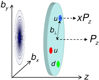
Figure 1: Illustration of a quark distribution in impact parameter space.

To give an example, the corresponding density for transverse polarization is given by

$$\rho(x,b_{\perp},s_{\perp},S_{\perp}) = \left\langle N_{\perp}\right|\int\limits_{-\infty}^{\infty}\frac{d\eta}{2\pi}e^{i\eta x}\overline{q}\big{(}\!-\!\frac{\eta}{2}n,b_{\perp}\big{)}\!\,\frac{1}{2}\big{[}\gamma^{+}-s_{\perp}^{j}i\sigma^{+j}\gamma_{5}\big{]}\,q\big{(}\frac{\eta}{2}n,b_{\perp}\big{)}\left|N_{\perp}\right\rangle$$

$$= \frac{1}{2}\left\{H(x,b_{\perp}^{2})+s_{\perp}^{i}S_{\perp}^{i}\left(H_{T}(x,b_{\perp}^{2})-\frac{1}{4m_{N}^{2}}\Delta_{b_{\perp}}\widetilde{H}_{T}(x,b_{\perp}^{2})\right)\right.$$

$$+ \frac{b_{\perp}^{j}\epsilon^{ji}}{m_{N}}\left(S_{\perp}^{i}E^{\prime}(x,b_{\perp}^{2})+s_{\perp}^{i}\overline{E}_{T}^{\prime}(x,b_{\perp}^{2})\right)+\left.s_{\perp}^{i}\frac{(2b_{\perp}^{i}b_{\perp}^{j}-b_{\perp}^{2}\delta^{ij})}{m_{N}^{2}}S_{\perp}^{j}\widetilde{H}_{T}^{\prime\prime}(x,b_{\perp}^{2})\right\}\,,$$

(65)

where the nucleon states are $\left|N_{\perp}\right\rangle=\left|P^{+},R_{\perp}=0,S_{\perp}\right\rangle$, and $f^{\prime}(b_{\perp}^{2})=\partial_{b_{\perp}^{2}}f(b_{\perp}^{2})$. The interpretation of the different GPDs becomes now very clear: While $H(x,b_{\perp}^{2})$ is the spherically symmetric charge distribution, the GPD $E(x,b_{\perp}^{2})$ is responsible for dipole-like distortions $\propto\mathbf{S}\times\mathbf{b}$ of the charge density. Similarly, the tensor GPD $E_{T}$ accounts for dipole-distortions of the form $\mathbf{s}\times\mathbf{b}$ for transversely polarized quarks.

Finally, the tensor GPDs $H_{T}$ and $\widetilde{H}_{T}$ contribute to the monopole structure $\propto\mathbf{S}\cdot\mathbf{s}$, and to the quadrupole distortion given by the last term in Eq. (65). Similar expressions hold for longitudinal polarizations [DH05], as well as for transversely polarized quarks in the pion [B⁺08h].

In particular with respect to lattice QCD calculations it is interesting to study $x$-moments of the density in Eq. (65). The first moment, $n=1$, is then entirely given in terms of nucleon vector, $F_{1,2}$, and tensor form factors (Fourier transformed to impact parameter space) and corresponds to the $x$-integrated density of quarks minus the density of anti-quarks, according to Eqs. (54),(56). All $n$-even moments are given by the sum of quark and anti-quark densities and are therefore strictly positive. We note that the probability density interpretation of GPDs, including the standard form factors as their first moments, in impact parameter space holds independently of a non-relativistic approximation or a special frame like the Breit-frame, in contrast to the classical interpretation of the three-dimensional Fourier-transforms introduced by Sachs [Sac62].

2.1.8 Fundamental sum rules

Based on Noethers theorem, fundamental momentum and spin sum rules can be derived [JM90, Ji97b] from the energy-momentum and angular momentum density tensor of QCD. Here, we will concentrate on the nucleon, but we note that it is straightforward to derive similar results for the pion as well as hadrons of higher spin. First we note that the off-forward nucleon matrix element of the gauge invariant, symmetric and traceless QCD energy-momentum tensor $T^{\mu\nu}$ can be parametrized in terms of three form factors $A(t)$, $B(t)$ and $C(t)$,

$$\langle N(P^{\prime})|T^{\mu\nu}|N(P)\rangle = \mathcal{S}_{\mu\nu}\overline{U}(P^{\prime})\left\{\gamma^{\mu}\overline{P}^{\nu}A(t)+\frac{i\sigma^{\mu\rho}\Delta_{\rho}}{2m_{N}}\overline{P}^{\nu}B(t)+\frac{\Delta_{\mu}\Delta^{\nu}}{m_{N}}C(t)\right\}U(P)\,,$$ (66)

where the energy-momentum tensor and the form factors in Eq. (66) contain implicit sums over all fundamental fields, i.e. the quarks and gluons. A comparison with the definition of the vector GPDs in Eq. (14) reveals that the form factors of the energy-momentum tensor are identical to the GFFs that parametrize the second, $(n\text{{=}}2)$-moments of the GPDs $H$ and $E$ (for quarks and gluons), see Eq. (30), i.e.

$$A(t)=A_{20}(t)\,,\quad B(t)=B_{20}(t)\,,\quad C(t)=C_{20}(t)\,.$$ (67)

Following Noethers theorem, the nucleon momentum sum rule can then be written as

$$1=A(0)=\sum_{q}A^{q}_{20}(0)+A^{g}_{20}(0)=\sum_{q}\langle x\rangle_{q}+\langle x\rangle_{g}\,,$$ (68)

which holds in practically identical form of course also for all other hadrons. For the spin-$1/2$ nucleon, the corresponding spin sum rule reads [Ji97b]

$$\frac{1}{2}=\frac{1}{2}\big{(}A(0)+B(0)\big{)}=\frac{1}{2}\big{(}\sum_{q}\langle x\rangle_{q}+\langle x\rangle_{g}+\sum_{q}B^{q}_{20}(0)+B^{g}_{20}(0)\big{)}\equiv\sum_{q}J_{q}+J_{g}\,,$$ (69)

and is therefore, in addition to the momentum fractions carried by the quarks and gluons, completely determined by the second moments of the GPDs $E^{q,g}(x,\xi,t)$ in the forward limit $\xi=0$, $t=0$, see Eq. (30). Furthermore, since the GFF $C_{20}(t)$ contributes with different sign to the second moments of the GPDs $H$ and $E$ in Eq. (30), we can also write the total quark and gluon angular momenta $J_{q,g}$ in Eq. (69) as

$$J_{q,g} = \frac{1}{2}\int_{-1}^{1}dxx\big{\{}H^{q,g}(x,\xi,0)+E^{q,g}(x,\xi,0)\big{\}}=\frac{1}{2}\big{(}A^{q,g}_{20}(0)+B^{q,g}_{20}(0)\big{)}\,,$$ (70)

which are independent of $\xi$. Clearly, the sum rules in Eq. (68) and (69) as well as the individual terms on their right hand sides are all gauge invariant. We note that $B(0)$ is called the anomalous gravitomagnetic moment [KO62, KZ70, Ter99, BHMS01] and, according to Eq. (68) and (69), has to vanish identically when summed over quarks and gluons,

$$B(0)=\sum_{q}B^{q}_{20}(0)+B^{g}_{20}(0)=0\,.$$ (71)

From a study of the underlying (local) QCD operators [Ji97b], one finds that the total quark angular momentum $J_{q}$ can be naturally decomposed,

$$J_{q} = \frac{1}{2}\Delta\Sigma+L_{q}\,,$$ (72)

in terms of the quark spin contribution, $\Delta\Sigma$, and the quark orbital angular momentum $L_{q}$, which are separately gauge invariant. As repeatedly stated in the literature, such a gauge invariant decomposition in terms of the gluon spin and OAM is not possible for $J_{g}$, using just local operators. However, one has to keep in mind that the gauge invariant and measurable gluon spin contribution, $\Delta G$, is given by the $x$-integral of the polarized distribution $\Delta g(x)$,

$$\Delta G=\int_{-1}^{1}dx\Delta g(x)\,,$$ (73)

which is in turn defined through a non-local gauge-invariant gluon operator. It is well known that the integration over $x$ of this non-local gluon spin operator cannot be analytically performed to obtain a gauge-invariant, local gluon spin operator [Jaf96]. In view of this, one might just define a gauge invariant gluon orbital angular momentum as [Ji97b]

$$L_{g} \equiv J_{g}-\Delta G\,.$$ (74)

We note that such a definition has been critically discussed in [BMN08]. In summary, based on Eqs. (69), (72) and (74), we can write down a decomposition of the nucleon spin,

$$\frac{1}{2} = \frac{1}{2}\Delta\Sigma+L_{q}+J_{g}$$

$$\bigg{(} = \frac{1}{2}\Delta\Sigma+L_{q}+\Delta G+L_{g}\bigg{)}_{\text{using Eq.~{}(\ref{Lg})}}\,,$$ (75)

where each term is separately gauge invariant and measurable. We would like to point out that the individual terms on the right hand side of Eq. (75) are scale, $\mu$, and scheme dependent in QCD. At least the quark spin and total angular momentum, $J_{q}$, are defined through nucleon matrix elements of local quark operators and are therefore directly calculable in lattice QCD.

2.1.9 Hadronic distribution amplitudes

Hadronic distribution amplitudes (DAs) $\phi(x,\mu)$ are universal, non-perturbative functions that play a fundamental role in hard exclusive processes and QCD-factorization theorems. Meson DAs in particular are essential ingredients in the description of heavy-to-light form factors in the framework of light cone sum rules, see, e.g., [BZ05], and in corrections to the “naive” factorization of non-leptonic decays of $B$-mesons to $\pi\pi$, $K\pi$ etc. [BBNS99, BBNS01] as well as radiative and semi-leptonic decays like $B\rightarrow\rho\gamma,K^{*}\gamma,\pi l\nu,\ldots$ [BFS01, AP02, BB02b] (for an overview we refer to Table 1 in [Ste03]). They are therefore of direct phenomenological importance for the study of $CP$-violation and the determination of CKM-parameters. Distribution amplitudes can be written as momentum integrals of Bethe-Salpeter wave functions $\varphi(x,k_{\perp})$, $\phi(x,\mu)\sim\int^{\mu^{2}}d^{2}k_{\perp}\varphi(x,k_{\perp})$, and have the interpretation of probability amplitudes for finding a parton with momentum fraction $x$ in a hadron at small transverse separation (related to the cut-off $\mu$) of the constituents. At very large momentum transfer $Q^{2}$, hadron form factors $F(Q^{2})$ can be written as convolutions of two corresponding distribution amplitudes and a hard scattering kernel $T$ that can be calculated perturbatively, $F(Q^{2})\sim\int dxdy\phi(x,Q^{2})T(x,y,Q^{2})\phi(y,Q^{2})$.

The distribution amplitude for, e.g., the $\pi^{+}$, $\phi_{\pi}(\xi)$, parametrizes the pion-to-vacuum matrix element of a bi-local light cone operator similar to the ones defined in Eq. (1),

$$\langle 0|\overline{d}(-z)\!\,\gamma^{\mu}\gamma_{5}\,\mathcal{U}_{[-z,z]}u(z)|\pi(P)\rangle = if_{\pi}P^{\mu}\int_{-1}^{1}d\xi e^{-i\xi P\cdot z}\phi_{\pi}(\xi)\,.$$ (76)

The DA $\phi_{K}(\xi)$ for a $K^{+}$ is defined in the same way, with replacements $d\rightarrow s$ and $f_{\pi}\rightarrow f_{K}$. Comparing with the standard definition of the pion and kaon decay constants, one finds

$$\int_{-1}^{1}d\xi\phi_{\pi,K}(\xi)=1\,.$$ (77)

The variables $x=(1+\xi)/2$ and $\overline{x}=1-x=(1-\xi)/2$ describe the longitudinal momentum fractions of the quark and the anti-quark in the meson. Higher moments of the DAs are defined by

$$\int_{-1}^{1}d\xi\xi^{n-1}\phi_{\pi,K}(\xi)=\langle\xi^{n-1}\rangle_{\pi,K}\,.$$ (78)

They parametrize meson-to-vacuum matrix elements of local quark operators, e.g. for the pion

$$\langle 0|\mathcal{S}_{\mu\mu_{1}\cdots\mu_{n-1}}\;\overline{d}\,\gamma_{\mu}\gamma_{5}\mskip 1.5mui{D^{\raisebox{2.41112pt}{$\scriptstyle\leftrightarrow$}}}{}^{\mu_{1}}\cdots\mskip 1.5mui{D^{\raisebox{2.41112pt}{$\scriptstyle\leftrightarrow$}}}{}^{\mu_{n-1}}\mskip 1.5muu-\text{traces}|\pi(P)\rangle = if_{\pi}P_{\mu}P^{\mu_{1}}\cdots P^{\mu_{n-1}}\langle\xi^{n-1}\rangle_{\pi}\,.$$ (79)

In the isospin-symmetric case one has $\phi_{\pi}(\xi)=\phi_{\pi}(-\xi)$, so that $\langle\xi^{2n-1}\rangle_{\pi}=0$. In the case of vector mesons, for example the $\rho$ and the $K^{*}$, two types of distributions amplitudes exist at twist-2 level, $\phi_{\|}(\xi)$ and $\phi_{\perp}(\xi)$. The DA $\phi_{\perp}(\xi)$ describes transversely polarized mesons and parametrizes matrix elements of the form $\langle 0|\overline{d}(-z)\Gamma\mathcal{U}_{[-z,z]}u(z)|\rho(P)\rangle$ where $\Gamma=i\sigma_{\mu\nu}$, and $\phi_{\|}(\xi)$ describes longitudinally polarized mesons, parametrizing matrix elements of vector and axial vector operators, $\Gamma=\gamma_{\mu}$ and $\Gamma=\gamma_{\mu}\gamma_{5}$, respectively. For details we refer to [BB96]. Distribution amplitudes can be conveniently expanded in terms of Gegenbauer polynomials $C_{n}^{3/2}(\xi)$,

$$\phi_{\pi,K}(\xi)=\frac{3}{4}(1-\xi^{2})\left\{1+\sum\limits_{n=1}^{\infty}a^{\pi,K}_{n}C_{n}^{3/2}(\xi)\right\}\,$$ (80)

where the Gegenbauer moments carry the full information about the scale dependence of the DA, $a^{\pi,K}_{n}=a^{\pi,K}_{n}(\mu^{2})$.

For the proton, one studies the nucleon-to-vacuum matrix element of a tri-local three-quark light-cone operator, given by [CZ84]

$$\epsilon^{abc}\langle 0|\left\{\mathcal{U}_{[z_{3},z_{1}]}u_{i}(z_{1})\right\}^{a}\left\{\mathcal{U}_{[z_{3},z_{2}]}u_{j}(z_{2})\right\}^{b}d_{k}(z_{3})^{c}|P,S\rangle\,,$$ (81)

where $z_{i}^{2}=0$, and Dirac and color indices are denoted by $i,j,k$ and $a,b,c$, respectively. The matrix element in Eq. (81) can be conveniently parametrized at leading twist in terms of an overall non-perturbative factor $f_{N}$, the nucleon ‘decay constant’, times vector, axial-vector and tensor Dirac structures, including the respective (Fourier-transformed) distribution amplitudes $V$, $A$ and $T$. Using isospin symmetry, it can be shown that at twist-2 level, all three amplitudes may be written in terms of just a single nucleon distribution amplitude $\varphi(x_{1},x_{2},x_{3})$, which is a function of the momentum fractions of the three valence quarks $x_{i}$, with $\sum_{i=1\ldots 3}x_{i}=1$ [Dzi88]. The moments of the proton DA are defined by

$$\varphi^{klm}=\int_{0}^{1}dx_{1}dx_{2}dx_{3}\delta\big{(}\sum_{i=1\ldots 3}x_{i}-1\big{)}x_{1}^{k}x_{2}^{l}x_{3}^{m}\varphi(x_{1},x_{2},x_{3})\,,$$ (82)

and parametrize proton-to-vacuum matrix elements of towers of local three-quark operators including covariant derivatives. Some more details will be given in section 5.2 below.

2.1.10 Polarizabilities

The electric polarizability describes the response of a hadron to an external electric field $\mathbf{E}$ in form of an induced electric dipole moment (EDM) $\mathbf{d}^{\text{ind}}=\alpha_{E}\mathbf{E}$. Similarly, an external magnetic field $\mathbf{B}$ induces a magnetic dipole moment proportional to the magnetic polarizability, $\boldsymbol{\mu}^{\text{ind}}=\beta_{M}\mathbf{B}$, in addition to the static magnetic moment related to the magnetic form factor, $\mu=G_{M}(Q^{2}=0)$.

In a low energy expansion in the photon energy $\omega$, the nucleon Compton scattering amplitude $T_{\text{Compt.}}$ to order $\mathcal{O}(\omega^{2})$ can be parametrized by the nucleon electric and magnetic polarizabilities, $\alpha_{E}$ and $\beta_{M}$,

$$T_{\text{Compt.}}=T_{\text{Compt.}}^{\text{point}}+\omega\omega^{\prime}\boldsymbol{\epsilon}^{\prime*}\cdot\boldsymbol{\epsilon}\,\alpha_{E}+\big{(}\mathbf{q}^{\prime}\times\boldsymbol{\epsilon}^{\prime*}\big{)}\cdot\big{(}\mathbf{q}\times\boldsymbol{\epsilon}\big{)}\,\beta_{M}+\mathcal{O}(\omega^{3})\,,$$ (83)

with photon polarization $\epsilon$ ( $\epsilon^{\prime}$) and four momentum $(\omega,\mathbf{q})$ ($(\omega^{\prime},\mathbf{q}^{\prime})$) of the incoming (outgoing) photon. Clearly, the polarizabilities describe the response of the nucleon to the electric ($\propto\omega\boldsymbol{\epsilon}$) and magnetic ($\propto\mathbf{q}\times\boldsymbol{\epsilon}$) components of the photon fields.

With respect to lattice calculations, it is important to note that the effects of the external fields can be accounted for by using an effective non-relativistic Hamiltonian with interaction term

$$H_{\text{eff}}^{\text{int}}=-\frac{1}{2}\big{(}\alpha_{E}\mathbf{E}^{2}+\beta_{M}\mathbf{B}^{2}\big{)}\,,$$ (84)

from which in particular the amplitude in Eq. (83) at low energies can be derived. The polarizabilities thus lead to shifts of the hadron masses of $\mathcal{O}(\mathbf{E}^{2},\mathbf{B}^{2})$ in the presence of external EM fields.

2.2 Hadron structure in experiment and phenomenology

Here we give a very brief overview of selected hadron structure observables in experiment and phenomenology.

2.2.1 Form factors and polarizabilities

The pion form factor $F_{\pi}(Q^{2})$ at low $Q^{2}\simeq 0.01,\ldots,0.3$ GeV² has been measured in experiments where a pion beam is scattered off the electrons of a liquid hydrogen target [A⁺86]. Investigations of the pion form factor in pion electroproduction, $ep\rightarrow e\pi^{+}n$, [B⁺78, A⁺78, B⁺79, V⁺01] at larger $Q^{2}\simeq 0.3,\ldots,10$ GeV² are based on the assumption of pion exchange dominance and described by quasi-elastic scattering on a virtual pion in the proton. These studies are in general subject to larger systematic uncertainties.

The magnetic moments of the proton and the neutron have been measured to excellent accuracy in experiments based on nuclear resonance [A⁺08i], $\mu_{p}=1+\kappa_{p}=2.7928$ and $\mu_{n}=-1.9130$. The isovector axial vector coupling constant is known to very high precision from neutron beta decay [A⁺08i], $g_{A}^{u-d}=g_{A}^{(3)}=a_{3}=1.2695(29)$. Using $SU(3)$ flavor symmetry, $g_{A}^{(3)}$ and the octet axial coupling constant, $g_{A}^{(8)}=a_{8}$, can be related to the hyperon decay constants $F$ and $D$ by $g_{A}^{(3)}=F+D$ and $g_{A}^{(8)}=3F-D$ [AEL95], which are measured to fair accuracy in hyperon $\beta$-decay [A⁺08i]. The proton and neutron electromagnetic form factors, i.e. Sachs’ form factors $G^{p,n}_{E,M}(Q^{2}=-t)$, at non zero momentum transfer are in general accessible in unpolarized elastic electron-nucleon scattering described by the standard Rosenbluth cross section. The results of these Rosenbluth-separation measurements have been improved and challenged in the last couple of years by experiments with polarized electron beams on polarized and unpolarized targets (beam-target asymmetry and polarization transfer measurements, respectively). For reviews of recent experimental results on nucleon EM form factors we refer to [HdJ04, PPV07, ARZ07]. In summary, results are available for

• $G^{p}_{E}$ from Rosenbluth-separation in a range of $Q^{2}\leq 0.1,\ldots,2$ GeV²

• $G^{p}_{M}$ from Rosenbluth-separation in a range of $Q^{2}\leq 0.1,\ldots,30$ GeV²

• $G^{n}_{M}$ from quasi-elastic electron scattering from deuterium (inclusive and with neutron tagging) using Rosenbluth-separation for $Q^{2}\leq 10$ GeV², however with increasing uncertainties for increasing values $Q^{2}$

• $G^{n}_{E}$ from polarization transfer and beam-target asymmetry measurements in a range of $Q^{2}\leq 0.1,\ldots,2$ GeV²

• $G^{p}_{E}/G^{p}_{M}$ from polarization transfer and beam-target asymmetry measurements in a range of $Q^{2}\leq 0.2,\ldots,6$ GeV²

Note that the Rosenbluth measurements of $G_{E}$ are limited to small $Q^{2}$ since the cross section is dominated by $G_{M}$ at large momentum transfers. Rosenbluth-separation analyses have in the past been based on the single-photon-exchange approximation. The difference that is seen for the ratio $G^{p}_{E}/G^{p}_{M}$ between Rosenbluth-separation and (beam and target) polarization measurements at large values of the momentum transfer squared might indicate that two-photon exchange contributions are non-negligible [GV03]. Further uncertainties in FF measurements are related to, e.g., nuclear effects in the analysis of electron scattering from deuterium and normalization uncertainties in the Rosenbluth-separation.

Assuming isospin symmetry, the charge weighted form factor results for the proton and neutron can be used to perform a flavor separation to obtain isovector and isosinglet or individual unweighted up- and down quark contributions, see Eq. 2.1.6.

Strange quark contributions to the form factors have been obtained from parity violating electron proton scattering. At present, experimental results for the strange quark contributions to the proton form factors are largely compatible with zero [A⁺07a, B⁺09b].

Proton electric and magnetic polarizabilities, $\alpha^{p}_{E}$ and $\beta^{p}_{M}$, are mainly known from real Compton scattering (RCS), e.g. at MAMI [OdL⁺01], with reasonable accuracy. Recent average values by the particle data group are $\alpha^{p}_{E}=(12.0\pm 0.5)10^{-4}\text{ fm}^{3}$ and $\beta^{p}_{M}=(1.9\pm 0.5)10^{-4}\text{ fm}^{3}$ [A⁺08i]. Experimental results for the neutron polarizabilities still suffer from rather large statistical and systematic uncertainties and do not yet provide a consistent picture. For reviews on nucleon polarizabilities, see e.g. [HdJ04, Sch05, DW08].

The pion polarizability, more precisely $\alpha^{\pi^{+}}_{E}-\beta^{\pi^{+}}_{M}$, has been determined from radiative pion photoproduction off the proton, $\gamma p\rightarrow\gamma\pi^{+}n$, at, e.g., MAMI [A⁺05a], and the scattering of pions on the Coulomb field of a large nucleus using the Primakoff effect at, e.g., Serpukhov [A⁺83, A⁺85]. Experiments using the Primakoff effect at COMPASS/CERN are ongoing. The situation is however somewhat unclear since the available results, which are based on different measurements and analysis methods, are not quite consistent within errors. For an overview of results from experiment and chiral perturbation theory calculations, see [GIS06].

2.2.2 PDFs and GPDs

Parton distribution functions (PDFs) of the nucleon are mainly accessible in deep inelastic lepton-nucleon scattering (DIS), semi-inclusive DIS (SIDIS), Drell-Yan lepton pair production and inclusive jet production in proton-(anti-)proton collisions. The basis of global PDF analyses are QCD factorization theorems, allowing to decompose cross sections and the corresponding structure functions in terms of hard scattering kernels and the PDFs, which parametrize the non-perturbative physics. The underlying perturbative QCD calculations of, e.g., the coefficient functions for unpolarized DIS and splitting functions for the evolution have already been pushed to impressive three-loop order (NNLO), see [VVM05] and references therein. Global phenomenological analyses of unpolarized PDFs have been carried out at NLO [MRST03, MRST04, N⁺08a, B⁺09a] and NNLO [AMP06, MSTW07, DDFL⁺07]. Recently, a first global analysis of polarized (helicity) PDFs at NLO has been presented [dFSSV08], and previous global analyses are described in [GRSV01, BB02a, LSS06]. From the phenomenological studies, unpolarized valence quark PDFs, $(u,d)(x)$, are known to high accuracy. Further results are available for the unpolarized antiquark, $(\overline{u},\overline{d})(x)$, and strange (sea) quark, $(s,\overline{s})(x)$, distributions, the corresponding polarized quark PDFs, as well as the unpolarized gluon distribution, $g(x)$. For a review of the spin structure of the proton and polarized PDFs we refer to [Bas05], and a discussion of recent progress in unpolarized PDFs can be found in [Sti08]. A precise measurement of the spin structure function $g_{1}(x)$ and corresponding results for the quark spin contributions to the nucleon spin have been recently reported by the HERMES collaboration [A⁺07b]. Despite enormous theoretical and experimental efforts over the last decade, the polarized gluon distribution, $\Delta g(x)$ is still only roughly constrained [HK08, A⁺08e, dFSSV08, A⁺08b]. Potential sources of uncertainties in global PDF analyses include contributions from higher twist, higher-order corrections, treatment of heavy flavors, and the need for phenomenological ansätze for the $x$-dependence of the PDFs at the input scale.

The $x$-moments of PDFs, which may be compared to lattice QCD calculations, can in principle be directly obtained by integrating the phenomenological PDFs (weighted with some power of $x$) over $x$. In practice, structure functions are of course only known for a certain range, $x=x_{\text{min}},\ldots,x_{\text{max}}$, due to a limited kinematical coverage in the experiments. The systematic uncertainty that is introduced by a necessarily model dependent extrapolation of the experimental results to $x=0$ and $x=1$, or by phenomenological parametrizations of the PDFs that determine (at least to some extent) their behavior for $x\rightarrow 0$ and $x\rightarrow 1$, is in general difficult to quantify.

Generalized parton distribution functions can be accessed in deeply virtual Compton scattering (DVCS) [MRG⁺94, Ji97a, Rad97, BMK02], wide-(large-) angle Compton scattering [DFJK99, Rad98], and related exclusive meson production processes. Of particular importance in the case of DVCS is the interference with the Bethe-Heitler (BH) process. The BH-amplitude can be described by the comparatively well-known nucleon form factors, see the discussion above. As usual, beam- and target-spin, as well as beam-charge asymmetries are constructed to reduce systematic uncertainties and to facilitate the analysis in terms of the individual unpolarized and polarized GPDs. A separation of contributions from up- and down-quark GPDs is attempted by using proton (hydrogen) and quasi-free neutron (deuterium) targets. First experimental DVCS results in form of the beam spin asymmetry have been presented in 2001 by HERMES at DESY [A⁺01] and CLAS at JLab [S⁺01]. Since then, much more results became available from measurements performed by the H1, ZEUS and HERMES collaborations at DESY (see, e.g., [C⁺03, A⁺05c, A⁺07c, A⁺08a]) and the Hall A and Hall B/CLAS collaborations at JLab (see, e.g., [MC⁺06, C⁺06b, G⁺08a]) . Recently, transverse (proton) target spin asymmetries measured at HERMES [A⁺08c] and DVCS cross section measurements with a longitudinally polarized beam on a neutron target at Hall A [M⁺07a] have been published and used to put first model dependent constraints on the total angular momentum of up- and down-quarks, $J_{u,d}$, in the proton. Compared to PDFs it turns out that the experimental and phenomenological analysis of GPDs is significantly more demanding. Based on a QCD factorization theorem [CFS97, CF99], DVCS and deeply virtual meson production at leading order can be described by complex valued Compton form factors of the form

$$\mathcal{H}(\xi,t)=\int^{1}_{-1}dx\left\{\frac{1}{\xi-x-i\epsilon}-\frac{1}{\xi+x-i\epsilon}\right\}H(x,\xi,t)\,,$$ (85)

and similar for the expressions involving the GPDs $E$, $\widetilde{H}$ and $\widetilde{E}$. The integration over $x$ clearly makes a direct extraction of GPDs as functions of the three variables $x$, $\xi$ and $t$ impossible (this is part of the “deconvolution problem” discussed in, e.g., [Die03]). Furthermore, the imaginary part of Eq.(85) is given by $\text{Im}\mathcal{H}(\xi,t)=\pi(H(\xi,\xi,t)-H(-\xi,\xi,t))$ and therefore only sensitive to the GPD at the crossover trajectory $x=\pm\xi$, so that only the real part of Eq.(85) may provide access to the full GPD $H(x,\xi,t)$ for $x\not=\xi$. However, using dispersion relations for the DVCS amplitude, it has been shown that the real part of Eq.(85) can be written as

$$\text{Re}\mathcal{H}(\xi,t)=\text{PV}\int^{1}_{-1}dx\left\{\frac{1}{\xi-x}-\frac{1}{\xi+x}\right\}H(x,x,t)+2\sum_{m=1}^{\infty}2^{2m}C_{2m,0}(t)\,,$$ (86)

where PV denotes the principle value of the integral, and the $C_{2m,0}(t)$ are the generalized form factors, contributing to higher moments $n=m+1$ of the GPDs $H$ and $E$ as in Eq. 30 for $n=2$. For studies of the analytic properties of the DVCS amplitudes, we refer to [Ter01, Ter05, DI07, Pol08, KMPK08]. In summary, one finds that DVCS and deeply virtual meson production at leading order only give access to GPDs at $x=\pm\xi$, apart from the contribution of the generalized form factors $C_{2m,0}(t)$ in Eq.(86). From the above discussion, it is clear that a description of these DVCS processes in terms of GPDs requires at least a partial modeling of their combined $x$-, $\xi$- and $t$-dependence. Attempts in this direction are for example described in [VGG99, GPV01, FMS03, DFJK05, GT06, AHLT07, AHLT09], and a more critical discussion of this topic can be found in [KMPK08]. For the above reasons, a direct comparison of moments of GPDs from lattice QCD and moments of the partially modeled GPDs has to be handled with some care.

Wide-angle Compton scattering, i.e. Compton scattering at large energy and momentum transfer squared, $s\sim|t|\sim|u|$, gives access to $1/x$-moments of GPDs at $\xi=0$, the so-called Compton form factors $R_{V}(t)=\int dxx^{-1}H(x,0,t)$, etc. [DFJK99, Rad98]. Measurements of wide-angle Compton scattering and also wide-angle meson photoproduction cross sections and helicity correlations could in particular help to understand the correlated $x$- and $t$-dependence of the GPDs. For a short review we refer to [Kro07] and references therein.

While PDFs of valence quarks in the pion, $q^{\pi}_{V}(x)$, can be well constrained from $\pi N$ DY lepton pair production [SMRS92, GRS99], the corresponding sea quark distribution can only be determined in a model dependent way [GRS99]. The distribution of gluons in the pion, $g^{\pi}(x)$, can be accessed in prompt photon production $\pi^{\pm}p\rightarrow\gamma X$ only at large $x$. An overview of early attempts to measure $g^{\pi}(x)$ can be found in [B⁺96]. The systematic uncertainties in the moments of pion PDFs obtained from such phenomenological analyses should be kept in mind when comparing to results from lattice QCD.

2.3 Hadrons in lattice quantum chromodynamics

2.3.1 Basics of lattice QCD

For an introduction to lattice gauge theories, we refer to the excellent monographs [Rot97, Rot05, Cre, MM, Smi02, DD].

Common to the observables discussed in the previous sections is that they share exact definitions in terms of hadronic matrix elements of QCD quark and gluon operators, which in turn can be written in the form of QCD path integrals. For a typical QCD correlator or expectation value, one has

$$\langle\mathcal{O}\rangle=\frac{1}{Z}\int[dq][d\overline{q}][dA]\;e^{iS_{QCD}[q,\overline{q},A]}\;\mathcal{O}\,,$$ (87)

where $\mathcal{O}$ consists of a product of quark and gluon fields, and

$$S_{QCD}=S_{q}+S_{g}=\int\!d^{4}x\left\{\overline{q}\left(i\not D-m\right)-\frac{1}{2}\text{Tr}F^{\mu\nu}F_{\mu\nu}\right\}\,,$$ (88)

denotes the standard continuum QCD action, where we have suppressed all flavor, Dirac and color indices for notational simplicity.

As a prerequisite for the numerical computation of the path integral, the theory is formulated in Euclidean space-time, as obtained from an analytic continuation to imaginary times, $t=x_{0}\rightarrow-it_{E}=-ix_{4}$, where $t_{E}$ is the real Euclidean time. Since $iS^{M}_{QCD}\rightarrow-S^{E}_{QCD}$, the Euclidean formulation avoids the oscillating exponential in Minkowski space-time that would prevent a numerical evaluation of the path integral. An ultra-violet regularization of the theory is provided by the discretization of space-time in form of a hypercubic lattice with lattice spacing $a$, corresponding to a cut-off $\mu=1/a$. An exactly local gauge invariant discretized path integral can be formulated in terms of discretized quark fields, $q(x=an)$, living on the lattice sites $n$, and the so-called link variables $U_{\mu}(an)=e^{iagA_{\mu}(an)}\in SU(3)$, which replace the gluon fields and which are connecting the sites, as illustrated in Fig. 2.

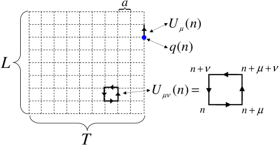
Figure 2: Illustration of basic lattice quantities.

We will set $a=1$ in the following for better readability and restore factors of $a$ later when necessary. For the correlator in Eq. (87), the discretization corresponds to the replacement

$$\langle\mathcal{O}\rangle\rightarrow\frac{1}{Z}\int\bigg{[}\prod_{i}dq(i)\bigg{]}\bigg{[}\prod_{j}d\overline{q}(j)\bigg{]}\bigg{[}\prod_{k,\mu}dU_{\mu}(k)\bigg{]}\;e^{-\sum_{n,m}\overline{q}(n)M_{n,m}q(m)-S_{g}[U]}\;\mathcal{O}\,,$$ (89)

where we have introduced the fermion matrix $M$. For, e.g., the standard Wilson gauge action we have

$$S_{g}^{W}[U]=\beta\sum_{P}\bigg{\{}1-\frac{1}{2N_{c}}\text{Tr}\big{(}U_{P}+U^{\dagger}_{P}\big{)}\bigg{\}}\,,$$ (90)

involving a sum over all distinct elementary plaquettes $U_{P}\hat{=}U_{\mu\nu}(n)$, which are built up from a product of four link variables as illustrated in Fig. 2. The coupling is given by $\beta=2N_{c}/g^{2}$. The Wilson gauge action reproduces the continuum action at small lattice spacings up to terms $\propto a^{2}$. The construction of a proper fermion action, i.e. $M_{n,m}$, is non-trivial. According to the Nielsen-Ninomiya theorem [NN81a, NN81b], it requires an explicit breaking of continuum chiral symmetry of the massless theory to obtain a theory that is free of fermion doublers, is local and leads to the correct equation of motion in the continuum limit. An introduction to chiral symmetry and lattice QCD is given in [CW04]. Different lattice actions that are used in practice will be discussed in the following section 2.3.2. We note that in general, improvement terms in the lattice action and the lattice operators are required to avoid discretization errors starting at $\mathcal{O}(a)$.

Most frequently, one is interested in correlators built up from quark fields $\mathcal{O}(n_{1},n_{2},\ldots)=q(n_{1})q(n_{2})\ldots\overline{q}(m_{1})\overline{q}(m_{2})\ldots$, for which one finds after integration over the Grassmann valued quark fields

$$\langle\mathcal{O}(n_{1},n_{2},\ldots)\rangle=\frac{1}{Z}\int\bigg{[}\prod_{k,\mu}dU_{\mu}(k)\bigg{]}e^{-S_{g}[U]}\det M[U]\sum_{\text{contract.}}M^{-1}_{n_{i},m_{j}}[U]M^{-1}_{n_{k},m_{l}}[U]\ldots\,,$$ (91)

where the sum runs over all contributing contractions of the $q(n_{i})$ and $\overline{q}(m_{j})$. The numerical integration over the link variables in Eq. (91) requires a finite lattice volume. Typical state-of-the-art lattice QCD simulations are performed for lattices of size, e.g., $L^{3}\times L_{t}=32^{3}\times 64$. The number of integration variables for such lattices is of the order of $32^{3}\times 64\times(N_{c}^{2}-1)\times 4\approx 67000000$, clearly showing that statistical methods must be employed. The basic idea is to generate a sequence or chain of so-called configurations ${U_{i}}$ where each $U_{i}$ represents link variables $U_{\mu}(n)$ for all $\mu$ and $n$, which sample the probability distribution given by $e^{-S[U]}$ (importance sampling). This can be achieved using a Markov-process (update-process) where the transition probability for going from one field configuration, $U$, to the next, $U^{\prime}$, satisfies detailed balance. Detailed balance can, for example, be implemented in form of the Metropolis algorithm (Metropolis accept-reject steps), where the new configuration $U^{\prime}$ is always accepted when the action decreases, and only accepted with probability $e^{-S[U^{\prime}]}/e^{-S[U]}<1$ when the action increases. However, the ordinary Metropolis algorithm will be extremely inefficient when non-local updates are required in the generation of the configurations, which is in particular the case when the full fermion determinant, $\det M[U]$, is taken into account. Non-local updates can be performed by evolving the system in a deterministic way in “simulation time” with finite time steps according to Hamiltonian equations of motion along a “classical” trajectory to a new field configuration, which is finally accepted or rejected based on the Metropolis acceptance test. Since the Hamiltonian for the evolved configuration stays close to its initial value, unacceptably high rejection rates as in the case of a random global change of the field configuration can be avoided. All this can be properly implemented in form of the widely used Hybrid Monte Carlo (HMC) algorithm, which is free of systematic errors. The effects of the fermion determinant can be included into the Hamiltonian and the HMC algorithm employing pseudo-fermionic fields and a corresponding pseudo-fermonic action. With an ensemble of $N_{\text{conf}}$ configurations $U_{i=1,\ldots,N_{\text{conf}}}$ generated by, e.g., the HMC algorithm, an estimate for the expectation value $\langle\mathcal{O}(n_{1},n_{2},\ldots)\rangle$ is given by

$$\langle\mathcal{O}(n_{1},n_{2},\ldots)\rangle\approx\overline{\mathcal{O}}(n_{1},n_{2},\ldots)=\frac{1}{N_{\text{conf}}}\sum_{i=1}^{N_{\text{conf}}}\sum_{\text{contract.}}M^{-1}_{n_{1},m_{1}}[U_{i}]M^{-1}_{n_{2},m_{2}}[U_{i}]\ldots\,,$$ (92)

with a statistical error proportional to $N_{\text{conf}}^{-1/2}$. A lattice QCD calculation of a correlator as in Eq. (92) therefore requires 1) the generation of a set of configurations, which is particularly expensive due to the presence of the fermion determinant $\det M[U]$, and 2) the computation of quark propagators $M^{-1}_{n,m}[U_{i}]$, i.e. the numerical inversion of the fermion matrix for a given ensemble of configurations. In the past, many lattice simulations have been done in the quenched approximation where $\det M[U]\rightarrow 1$, corresponding to neglecting sea quark loops, in order to reduce the computational expense. The quenched approximation is not a controlled approximation and only becomes exact in the limit of infinitely heavy quarks, which is why dynamical (unquenched) calculations including the full fermion determinant are indispensable.

A typical $N_{f}=2+1$ lattice QCD calculation with two light (up and down) and one heavier (strange) quark involves three dimensionless input parameters (assuming fixed spatial, $L$, and temporal, $L_{t}$, lattice extents): The coupling constant $\beta$ in the gauge action, Eq. (90), and the quark masses $m_{u}=m_{d}$ and $m_{s}$ in the fermion determinant. The calculation of dimensionful quantities requires the determination of the lattice spacing $a$ in physical units, which can only be done a posteriori by a matching of lattice results for e.g. the mass of the nucleon or the rho, or the heavy quark quark potential at the “Sommer scale” [Som94], with results from experiment and/or phenomenology. The determination of the lattice scale is therefore subject to, and a source of, statistical and systematic uncertainties.

Costs of dynamical fermion simulations typically rise approximately with some power of the lattice extent $L$ and powers of the inverse lattice spacing and the inverse light quark mass. Until a couple of years ago, unquenched simulations where found to be restricted to the “heavy quark” regime, corresponding to pseudoscalar (pion) masses in a range of $m_{\pi}\approx 600\text{ MeV}\ldots 1000\text{ MeV}$. Due to the predicted rise of cost with powers of $1/m_{q}$, $L$ and $1/a$, simulations below $m_{\pi}\approx 300\text{ MeV}$, let alone close to the physical pion mass, were regarded as unattainable. However, due to ongoing progress in the development of machines and the resulting increase in computer power, significantly improved algorithms and other conceptual advances, lattice hadron structure calculations at pion masses of around $300\text{ MeV}$ actually became feasible during the recent years. Based on these developments, current predictions are way more optimistic than before, giving hope that in the not-too-far future lattice hadron structure calculations of selected observables may be possible with reasonable statistics close to or even directly at the physical pion mass. For a recent review of the status of lattice QCD simulations, including cost estimates, we refer to [Jan08].

Concerning the investigation of the structure of hadrons, the choice of the lattice parameters and the lattice size is roughly speaking a two-scales problem. On the one hand, the quark masses and/or the lattice extent must be sufficiently large so that not only the hadron under investigation, but also other relevant degrees of freedom, in particular the virtual pions (the “pion cloud”), which are essential for the hadron structure, fit into the lattice volume. At the same time, the lattice spacing should be small enough (the coupling large enough) so that the internal structure of the hadron can be resolved in the first place and discretization effects can be kept under control. The spatial dimensions of the relevant states may be measured in terms of their de Broglie wavelengths and rms radii. As a rule of thumb it is often required that $m_{\pi}L\geq 4$, but if this is sufficient to suppress finite volume effects clearly must be studied case-by-case and will depend on the observable under consideration. Typical lattice spacings are $a\approx 0.1\text{ fm}$ or smaller, which may be compared to the rms radius of, e.g., the nucleon at currently accessible quark masses on the lattice, which is $\langle r^{2}\rangle^{1/2}\approx 0.5\text{ fm}$. A further restriction in conventional lattice hadron structure calculations comes from the fact that the lattice momenta accessible in a finite volume, $V=L^{3}$, are discrete and given by $p=2\pi n/(aL)$, $-L/2\leq n\leq L/2$, for periodic boundary conditions in spatial directions, i.e. $q(\vec{x}+L\vec{e}_{j})=q(\vec{x})$ for quark fields. This leads to lowest non-vanishing momentum components ($n=1$) that are rather large, $p\gtrapprox 0.3\text{ GeV}$.

In order to finally obtain predictions at the physical point, the continuum and infinite volume limits have to be taken, and the quark masses eventually have to be tuned to their physical values. The continuum limit is in general achieved by tuning the coupling to the value where the lattice correlation length, generically given by the inverse mass gap in lattice units, $\xi^{\text{lat}}=(aE-aE_{0})^{-1}=(am)^{-1}$, diverges, such that the physical (continuum) mass stays finite. In practice, the expected discretization errors of the lattice results proportional to $a$ or $a^{2}$ may be studied directly by performing simulations at different couplings $\beta$, and the continuum limit can be taken by performing extrapolations in the lattice spacing. As will be briefly discussed in section 2.4 below, extrapolations to $a=0$, $L=\infty$, and in particular $m^{\text{lat}}_{q}=m^{\text{phys}}_{q}$ may be systematically studied in the framework of the low energy effective field theory of QCD. In summary, lattice QCD simulations are subject to a number of statistical and systematic uncertainties:

• statistical errors from the Monte Carlo evaluation of the path-integral

• discretization effects due to finite lattice spacing

• finite size (volume) effects due to finite lattice volume

• large unphysical quark (pion) masses

• statistical and systematic errors in the setting of the lattice scale

Additional uncertainties in hadron structure observables arise for example in the calculation of lattice renormalization constants, from contributions of excited states to hadron correlation functions and from extrapolations required by large lowest non-vanishing lattice momenta. Of central importance is that all these uncertainties can at least in principle be systematically and continuously reduced by using larger ensembles of configurations, reducing the lattice spacing (increasing the coupling), increasing the lattice size, and lowering the quark masses. This is different from model calculations, which certainly can and in many cases do provide a better understanding of how QCD works, but generically suffer from uncontrollable systematic uncertainties.

2.3.2 Lattice actions: Overview

Gauge actions

Starting from the original Wilson gluon action in Eq. (90), many $\mathcal{O}(a^{n})$-improved gauge actions have been introduced over the years. This is systematically described in the form of the Symanzik improvement program [Sym83a, Sym83b]. A large variety of gauge field actions have been used in large scale lattice simulations, mostly differing in the numerical values of certain improvement coefficients. For example, the standard Wilson gauge action has been used in dynamical Wilson fermion simulations by QCDSF/UKQCD since 2000 [Stü01, Irv01] and by JLQCD [A⁺03]. A tree-level Symanzik improved action is employed by ETMC [Urb07] in dynamical Wilson twisted mass fermion simulations, and by QCDSF in recent dynamical Wilson fermion studies [C⁺09]. Simulations by MILC are based on a one-loop Symanzik improved action with Asqtad staggered quarks, see [B⁺01, A⁺04] and references therein. A tapole-improved Symanzik action was used in [Z⁺02]. Similar (renormalization-group improved) gauge actions in the form of the Iwasaki action were used in, e.g., dynamical overlap fermion simulations by JLQCD [A⁺08l], Wilson fermion simulations by PACS-CS [A⁺08k] and domain wall fermion calculations by RBC/UKQCD [A⁺08h], and in the form of the doubly-blocked Wilson (DBW2) action by RBC [A⁺05e].

A further way of improving lattice simulations, for example concerning chiral properties of Wilson fermions and taste symmetry breaking of staggered fermions, is to replace the original “thin” link variables by so-called fat or smeared gauge links. Smeared links can be iteratively constructed by replacing each link by a weighted average of the link and nearby gauge paths represented by products of three or more links (e.g. staples). Typical examples are APE smearing [A⁺87] and HYP blocking/smearing [HK01], where the latter only includes staples that lie within the hypercube attached to the original gauge link. The differentiable stout smearing [MP04] has been used in a number of recent studies [D⁺08c, L⁺09, C⁺09], and a differentiable form of APE smearing was proposed in [KLW04] in the context of Fat Link Clover Improved (FLIC) fermions [Z⁺02].

Smearing generically suppresses short-range fluctuations of the gauge fields and is therefore useful in many practical applications.

Lattice fermions

Wilson fermions [Wil] are numerically simple to implement, well understood and tested, and cost-efficient for not too small quark masses. The Wilson fermion action action is obtained by adding the so-called Wilson term of the form $-ar/2\sum_{n}\overline{q}(n)\!\boxempty\!q(n)$ to the naively discretized action. The Wilson term removes the fermion doubler modes and vanishes in the continuum limit, but breaks chiral symmetry explicitly at finite lattice spacing. The Wilson fermion action can be written as

$$S^{WF} = \frac{1}{2\kappa}\sum_{n,m}\overline{q}(n)M_{n,m}q(m)\,,$$ (93)

with

$$M_{n,m}=\delta_{nm}-\kappa\sum_{\mu}\bigg{\{}(r-\gamma_{\mu})U_{\mu}(n)\delta_{n+\hat{\mu},m}+(r+\gamma_{\mu})U^{\dagger}_{\mu}(n-\hat{\mu})\delta_{n-\hat{\mu},m}\bigg{\}}$$ (94)

where $\hat{\mu}$ denotes a unit vector in $\mu$-direction, $r$ is the Wilson parameter (in most applications $r=1$), and the hopping parameter $\kappa$ is defined by $\kappa=(8r+2m_{q})^{-1}$. Lattice spacing errors for Wilson fermions are generically of $\mathcal{O}(a)$. The Wilson fermion action can be $\mathcal{O}(a)$-improved using the so-called clover term $ia/4c_{SW}\sum_{n}\overline{q}(n)\sigma_{\mu\nu}F_{\mu\nu}(n)q(n)$ [SW85] with a properly discretized field strength tensor. The $\mathcal{O}(a)$-improvement can be achieved numerically by tuning the Sheikholeslami-Wohlert coefficient $c_{SW}$. Wilson fermions are used in large scale numerical simulations by, e.g., QCDSF/UKQCD with $n_{f}=2$ flavors [Stü01, Irv01], QCDSF with $n_{f}=2+1$ flavors[G⁺07e], and PACS-CS with $n_{f}=2+1$ flavors [A⁺08k]. Due to improved methods, e.g. the rational hybrid Monte Carlo (RHMC) algorithm [CK04], mass preconditioning and Hasenbusch acceleration [Has01], it is by now feasible to employ Wilson fermions at low quark masses where $m_{\pi}<300$ MeV.

In their original form, Wilson fermions suffer from additive quark mass renormalization, which leads in particular to numerical instabilities in simulations at small quark masses. This can be avoided by working with twisted-mass Wilson Fermions, which can be obtained by adding a twisted mass term of the form $i\mu_{q}\overline{q}\gamma_{5}\tau_{3}q$ to the Wilson fermion action [FGSW01], with mass parameter $\mu_{q}$, and where $\tau_{3}$ acts in flavor space. Another advantage of twisted mass fermions is that discretization errors for many observables can be reduced to be $\mathcal{O}(a^{2})$ by tuning the bare quark mass to its critical value, i.e. when working at so-called ‘maximal twist’ [FR04]. On the downside, the twisted mass term leads to a violation of isospin and parity symmetry at $\mathcal{O}(a^{2})$. Twisted mass Wilson fermions are cost-efficient and used in large scale numerical simulations by the ETMC [Urb07]. A review of twisted mass lattice QCD is given in [Shi08].

Staggered (Kogut-Susskind) fermions represent another highly cost-efficient fermion discretization that is free of the usual doublers and possesses a remnant chiral symmetry for vanishing quark masses, which is sufficient to prevent additive quark mass renormalization. However, staggered fermion fields carry an additional (unphysical) quantum number called ‘taste’. The four different tastes of staggered fermions complicate the physical interpretation of the results, and in many practical applications the fourth root of the staggered fermion determinant is taken in order to reduce the four taste degrees of freedom to a single fermionic DOF. The validity of this ‘fourth-root-trick’ is currently under intense debate, see [BGSS08, Cre08] and references therein. Staggered fermions have been widely used in numerical simulations over the last decade by the MILC collaboration in the form of the Asqtad (a-squared tadpole improved) staggered quark action [B⁺01, A⁺04]. The lowest pion masses that have been reached are $m_{\pi}\approx 270$ MeV.

Recently, interest has shifted towards using chiral (or Ginsparg-Wilson [GW82]) fermions in large scale lattice simulations. The Dirac operator $D$ of chiral fermions is required to satisfy the Ginsparg-Wilson relation $\{D,\gamma_{5}\}=aD\gamma_{5}D$, which has a non-zero RHS at finite lattice spacing, corresponding to broken continuum chiral symmetry. However, GW-fermion theories are invariant under a lattice chiral symmetry transformation [Lüs98], which is not only appealing from a theoretical point of view, but also proves beneficial for a number of practical reasons: The fermion action is automatically $\mathcal{O}(a)$ improved, operator renormalization is simplified by reduced/eliminated mixing of operators (operator renormalization will be discussed in the following sections), it is in particular guaranteed that the vector and axial-vector current renormalization constants agree, $Z_{A}=Z_{V}$, and additive quark mass renormalization is absent. The two types of chiral fermions that are employed in numerical simulations are domain wall [Kap92] and overlap fermions [Neu98]. At the moment, computational resources are not sufficient as to allow for full overlap fermion simulations. Overlap fermion calculations by JLQCD have been performed in a fixed topological sector [A⁺08l]. Domain wall (DW) fermions are formulated in 5 dimensions, and provide the full lattice chiral symmetry only when the extent of the fifth dimension, $L_{5}$, is approaching infinity. They have the advantage that $L_{5}$ can be tuned to achieve a compromise between residual chiral symmetry breaking on the one hand and computational cost on the other. In typical DW lattice simulations $L_{5}=16$ or $32$, with pion masses as low as $m_{\pi}\approx 300$ MeV. Domain wall fermions have been employed by RBC in simulations with $n_{f}=2$ [A⁺05e], and by RBC/UKQCD with $n_{f}=2+1$ [A⁺08h] flavors.

In the ideal case, the fermion action that is being used for the computation of the lattice gauge configurations (i.e. including the fermion determinant) is identical to the fermion action that is being used for the calculation of quark propagators. In other words, one consistently uses the same type of lattice fermion for the sea and valence quarks. In order to benefit from the numerical efficiency of, e.g., Wilson or staggered fermions, and at the same time from the desired chiral properties of overlap or DW fermions, so-called hybrid or mixed action schemes have been devised, where cost-efficient fermion discretizations are used for the time-consuming and expensive calculation of the gauge configurations, and where the quark propagators are based on chiral fermion formulations. In this case, the valence bare quark masses may be tuned in order to match the masses of mesons and baryons in the pure sea quark and hybrid formulations. One has to keep in mind, however, that mixed action simulations suffer from unitarity violation at finite lattice spacing. Mixed action calculations have been performed by, e.g., the LHPC collaboration [H⁺08a, WL⁺08], using domain wall valence fermions in combination with Asqtad staggered sea quarks of the gauge configurations provided by MILC.

2.3.3 Basic methods and techniques

An excellent introduction to lattice hadron structure calculations can be found in [Hor00]. Below, we only briefly introduce some of the basic methods and techniques employed in numerical studies of hadrons in lattice QCD.

Two- and three-point functions

Lattice studies of hadron matrix elements introduced in section 2.1 are mostly based on hadron two- and three-point functions. Two-point functions have the following form:

$$C_{\text{2pt}}(t,\mathbf{P}) = \langle h(t,\mathbf{P})h^{\dagger}(0,\mathbf{P})\rangle\,.$$ (95)

Here $h^{\dagger}(t,\mathbf{P})$ and $h(t,\mathbf{P})$ are interpolating fields for the source and sink, respectively, of a hadron with lattice momentum $\mathbf{P}$ at the Euclidean time $t$. The interpolating fields are given by products of quark fields, which are combined in color, Dirac and flavor space in order to provide the quantum numbers of the hadron under consideration. The exact form of the interpolating field for a given hadron is not unique. With $h(t,\mathbf{P})=\sum_{\mathbf{x}}e^{-i\mathbf{x}\cdot\mathbf{P}}h(t,\mathbf{x})$, standard choices for the $\pi^{+}$, the proton, $p$, and the $\rho^{+}$ are

$$\pi^{+}\big{(}J^{P}=0^{-}\big{)} : \quad h(t,\mathbf{x})=\overline{d}(t,\mathbf{x})[\gamma_{4}]\gamma_{5}u(t,\mathbf{x})\,,$$ (96)

$$p\big{(}J^{P}=\text{$\frac{1}{2}$}^{+}\big{)} : \quad h_{i}(t,\mathbf{x})=\epsilon_{abc}\left\{u^{a}(t,\mathbf{x})^{T}C\gamma_{5}d^{b}(t,\mathbf{x})\right\}u^{c}_{i}(t,\mathbf{x})\quad i=1\ldots 4\,,$$ (97)

$$\rho^{+}\big{(}J^{P}=1^{-}\big{)}) : \quad h_{j}(t,\mathbf{x})=\overline{d}(t,\mathbf{x})\gamma_{j}u(t,\mathbf{x})\quad j=1\ldots 3\,$$ (98)

where $[\gamma_{4}]$ indicates the possibility to include $\gamma_{4}$, and $C$ denotes the charge conjugation matrix. It should be noted that the interpolating field in Eq.(97) has no definite parity, and a projection operator may be used to suppress the negative parity contributions, see below. A Rarita-Schwinger interpolating field for, e.g., the spin-$3/2$ $\Delta^{+}$-baryon is given by

$$\Delta^{+}\big{(}J^{P}=\text{$\frac{3}{2}$}^{+}\big{)}:\quad h_{i,\alpha}(t,\mathbf{x}) = \epsilon_{abc}\bigg{(}2\left\{u^{a}(t,\mathbf{x})^{T}C\gamma_{\alpha}d^{b}(t,\mathbf{x})\right\}u^{c}_{i}(t,\mathbf{x})$$ (99)

$$+ \left\{u^{a}(t,\mathbf{x})^{T}C\gamma_{\alpha}u^{b}(t,\mathbf{x})\right\}d^{c}_{i}(t,\mathbf{x})\bigg{)}\quad i=1\ldots 4\,.$$

Clearly, these interpolating fields do not directly create the physical pion, nucleon, $\rho$-meson and $\Delta$-baryon ground states. However, they do have a non-zero overlap with the physical states, which can be enhanced by using spatially smeared instead of point-like quark fields,

$$q^{S}(t,\mathbf{x})=\sum_{\mathbf{y}}H(\mathbf{x},\mathbf{y},t;[U])q(t,\mathbf{y})\,,$$ (100)

where the smearing kernel $H$ is hermitian and transform as

$$H(\mathbf{x},\mathbf{y},t;[U])\rightarrow G(\mathbf{x},t)H(\mathbf{x},\mathbf{y},t;[U])G^{-1}(\mathbf{y},t)\,$$ (101)

under gauge transformations. In practice, the source and sink smearing is often implemented in form of the iterative Jacobi smearing [A⁺93], which depends on two smearing parameters. These parameters can be tuned to provide an optimal overlap with the physical hadron wave function.

Hadron three-point functions are given by

$$C^{\mathcal{O}}_{\text{3pt}}(\tau,\mathbf{P}^{\prime},\mathbf{P}) = \langle h(\mathbf{P}^{\prime},t_{\text{snk}})\sum_{\mathbf{x}}e^{i\mathbf{x}\cdot\mathbf{\Delta}}\mathcal{O}(\tau,\mathbf{x})h^{\dagger}(\mathbf{P},0)\rangle\,,$$ (102)

describing a hadron that is probed by an operator $\mathcal{O}(\tau,\mathbf{x})$ at time $\tau$, which is Fourier transformed with respect to $\mathbf{x}$ to momentum space with a momentum transfer $\mathbf{\Delta}=\mathbf{P}^{\prime}-\mathbf{P}$.

The Euclidean time dependence of two- and three-point functions can be obtained by inserting time translation operators, $\exp(-\hat{P}_{4}t)$, to shift the interpolating fields to $t=0$, and by inserting complete sets of energy-momentum eigenstates, $|E_{m}(\mathbf{P})\rangle$, into Eqs. (95) and (102). One obtains for the pion

$$C^{\pi}_{\text{2pt}}(t,\mathbf{P}) = Z(P)\big{\{}e^{-E(\mathbf{P})t}+e^{-E(\mathbf{P})(T-t)}\big{\}}+\cdots=2Z(P)\cosh((T/2-t)E(\mathbf{P}))+\cdots$$

$$C^{\pi,\mathcal{O}}_{\text{3pt}}(\tau,\mathbf{P}^{\prime},\mathbf{P}) = \big{(}Z(P^{\prime})Z(P)\big{)}^{1/2}\langle\pi(\mathbf{P^{\prime}})|\mathcal{O}(0)|\pi(\mathbf{P})\rangle\times$$ (106)

$$\left\{\begin{array}[]{c}e^{-(t_{\text{snk}}-\tau)E(\mathbf{P^{\prime}})-\tau E(\mathbf{P})}+\cdots\quad,t_{\text{snk}}\geq\tau\\ (-1)^{n_{4}+n_{5}}e^{-(\tau-t_{\text{snk}})E(\mathbf{P^{\prime}})-(T-\tau)E(\mathbf{P})}+\cdots\quad,T\geq\tau\geq t_{\text{snk}}\end{array}\right.\,,$$

where $T$ denotes the time extent of the lattice, $T\geq t_{snk}$, while $n_{4}$ and $n_{5}$ are the number of $\gamma_{4}$ and $\gamma_{5}$ matrices, respectively, in the operator. Contributions from excited states with energies $\ldots>E^{\prime\prime}>E^{\prime}$ and from wrap-around effects are denoted by the dots in Eqs.(LABEL:C2ptPi,106). For e.g. $t_{\text{snk}}\geq\tau$, they are suppressed if $T-t,t,\tau\gg(E^{\prime}-E)^{-1}$ and $t_{\text{snk}}-\tau\gg(E^{\prime}-E)^{-1}$. The nucleon two-point function can be written as

$$C^{N}_{\text{2pt};i,j}(t,\mathbf{P}) = \big{(}Z(P)\overline{Z}(P)\big{)}^{1/2}\sum_{S}\big{\{}\overline{U}_{i}(P,S)U_{j}(P,S)e^{-E(\mathbf{P})t}\big{\}}+\cdots\,.$$ (107)

where the dots represent contributions due to wrap-around effects (e.g. anti-nucleons moving in opposite time direction) that are suppressed for $T\gg E^{-1}$, and from excited states, for example the first excited positive parity state corresponding to the Roper resonance $N(1440)$, that are suppressed for $t\gg(E^{\prime}-E)^{-1}$. Contributions from negative parity partners, for example the $N^{*}(1535)$ resonance, and anti-nucleons are additionally suppressed by projection onto the upper Dirac components,

$$C^{N}_{\text{2pt};\Gamma_{\text{unpol}}}(t,\mathbf{P})=\text{Tr}\big{(}\Gamma_{\text{unpol}}C^{N}_{\text{2pt}}(t,\mathbf{P})\big{)}\,,$$ (108)

where $\Gamma_{\text{unpol}}=(1+\gamma_{4})/2$. The nucleon three-point function can be written as

$$C^{N,\mathcal{O}}_{\text{3pt};\Gamma_{\text{pol}}}(\tau,\mathbf{P}^{\prime},\mathbf{P}) = e^{-(t_{\text{snk}}-\tau)E(\mathbf{P^{\prime}})-\tau E(\mathbf{P})}\big{(}\overline{Z}(P^{\prime})Z(P)\big{)}^{1/2}\times$$ (109)

$$\sum_{S,S^{\prime}}\text{Tr}\big{\{}\Gamma_{\text{pol}}\overline{U}(P,S)U(P^{\prime},S^{\prime})\big{\}}\langle P^{\prime},S^{\prime}|\mathcal{O}(0)|P,S\rangle+\cdots\,,$$

where we have introduced a polarized projector $\Gamma_{\text{pol}}$, e.g. $\Gamma_{\text{pol}}=\Gamma_{\text{unpol}}(1-\gamma_{5}\gamma_{3})/2$, which suppresses contributions from negative parity states and at the same time allows to access the spin structure of the nucleon. The two- and three-point functions for spin-1 states like the $\rho$-meson can be written in a way similar to the pion correlators in Eq.(106), except for the appearance of polarization vectors $\epsilon_{j}(\mathbf{P^{\prime}})^{*}$ and $\epsilon_{i}(\mathbf{P})$ for the sink and source, respectively, see, for example, Ref. [H⁺07b]. The corresponding formalism for spin-$3/2$ $\Delta$-baryon correlators can be found in [LDW92].

Lattice calculations of two-point functions clearly provide access to the spectrum of mesons and baryons, including hybrid and exotic states via the exponential decay in the Euclidean time $t$. Particularly relevant for hadron structure calculations discussed in this work are of course the masses (and dispersion relations) of the respective ground states, which may be directly obtained from plateaus in the effective mass $m_{\text{eff}}(t)=\ln C_{\text{2pt}}(t-1,\mathbf{0})/C_{\text{2pt}}(t,\mathbf{0})$, or from (multi-) exponential fits to the two-point functions. The hadron three-point functions in Eqs.(106) and (109) give direct access to the hadron matrix elements of the local quark operators that have been discussed in section 2.1, and thereby the form factors and generalized form factors that parametrize the non-perturbative physics. One option to extract the lattice estimates of the hadronic matrix element is to perform simultaneous fits to the time dependences of the two- and three-point functions, based on Eqs. (106), (or (107), (109)), possibly also including excited state contributions, with energies $E(\mathbf{P}),E(\mathbf{P}^{\prime}),\ldots$, overlap factors $Z$, and the sought-after matrix elements $\langle h(P^{\prime})|\mathcal{O}|h(P)\rangle$ as fitting parameters. In the case that a spin-projection has been used in the hadron three-point function, for example as for the nucleon in Eq. (109), the extracted hadron matrix element will be understood as implicitly including this spin-projection. Alternatively, ratios of three- and two-point functions can be constructed in order to remove overlap and exponential factors in Eqs. (106) and (109). An often used ratio is

$$R_{\mathcal{O}}(\tau,P^{\prime},P)=\frac{C^{\mathcal{O}}_{\text{3pt}}(\tau,\mathbf{P}^{\prime},\mathbf{P})}{C_{\text{2pt}}(t_{\text{snk}},\mathbf{P}^{\prime})}\left[\frac{C_{\text{2pt}}(t_{\text{snk}}-\tau,\mathbf{P})\;C_{\text{2pt}}(\tau,\mathbf{P}^{\prime})\;C_{\text{2pt}}(t_{\text{snk}},\mathbf{P}^{\prime})}{C_{\text{2pt}}(t_{\text{snk}}-\tau,\mathbf{P}^{\prime})\;C_{\text{2pt}}(\tau,\mathbf{P})\;C_{\text{2pt}}(t_{\text{snk}},\mathbf{P})}\right]^{1/2}\,,$$ (110)

which is approximately time-independent, i.e. exhibits a plateau in $\tau$, for an operator insertion sufficiently far away from source and sink, $t_{\text{snk}}\gg\tau\gg 0$. Note that this holds for arbitrary choices of momenta $P$ and $P^{\prime}$ (in particular $P\not=P^{\prime}$), projectors $\Gamma$, and operators $\mathcal{O}$. The situation is slightly different for the pion, since pion masses in modern lattice calculations are approaching values for which wrap-around effects are in general non-negligible, i.e. where the full $\cosh(T/2-t)$ time dependence of the pion two-point functions has to be taken into account. In this case, a residual time dependence of $R_{\mathcal{O}}(\tau,P^{\prime},P)$ remains, which is however well understood and, up to small systematic errors, does not spoil the usefulness of the ratio. Different ratios have been used in the literature, see, e.g., [WDL92, LDW92, H⁺07b, BFJ⁺07]. A salient feature of ratios as in Eq.(110) is that statistical fluctuations of the involved quark propagators in the numerator and denominator cancel out to some extent. On the other hand, the square root in Eq.(110) poses a potential disadvantage as two-point functions at or close to $t_{\text{snk}}$ (where they are most noisy) may take values that are very close to zero or even negative, in which case it is not clear what to do with the square root of a negative number. This does happen in practice in particular at large momenta, and in such cases it is most safe to exclude the corresponding two-point functions/hadron momenta from the analysis. An alternative way of dealing with this problem using shifted two-point functions has been suggested and used in [B⁺07f]. Once a plateau in the ratio Eq. 110 has been identified, an average may be taken to increase the statistics, and a lattice estimate of the hadronic matrix element is then given by

$$\langle h(P^{\prime})|\mathcal{O}|h(P)\rangle_{\text{lat}}=C(P^{\prime},P)\frac{1}{\tau_{\text{max}}-\tau_{\text{min}}+1}\sum_{\tau=\tau_{\text{min}}}^{\tau_{\text{max}}}R_{\mathcal{O}}(\tau,P^{\prime},P)\,,$$ (111)

where $C(P^{\prime},P)$ is a known kinematical coefficient.

The lattice estimate of $\langle h(P^{\prime})|\mathcal{O}|h(P)\rangle$ (which may already include a spin projection) obtained from Eq. 111, or from a simultaneous fit to the two- and three-point functions as described above, can then be set equal to the corresponding continuum parametrization of the hadron matrix element in terms of (generalized) form factors, as given in Eqs. (8,9,10,11,20,21,22,…). Since the lattice momenta $\mathbf{P},\mathbf{P}^{\prime}$ are discrete, only specific values of the squared momentum transfer $t=\Delta^{2}=(P^{\prime}-P)^{2}$ can be reached. Typically, several different combinations of the accessible $\mathbf{P},\mathbf{P}^{\prime}$, e.g. all $L/(2\pi)\mathbf{P}=(\pm 1,0,0),(0,\pm 1,0),(0,0,\pm 1)$ for fixed $\mathbf{P^{\prime}}=2\pi/L(0,0,0)$, give the same value of $t$. Furthermore, we note that the (generalized) form factors for a given hadron and type of operator (vector, axial-vector, tensor operator with $l$-derivatives) by definition only depend on $t$ (or $Q^{2}$), but are in particular independent of the hadron spins $S,S^{\prime}$ (or the spin-projection) and of the specific indices $\mu,\nu,\mu_{1},\ldots$ of the local operators given in Eq. (3). For a given value of $t$, it is therefore possible to construct a set of equations of the form “$\langle h(P^{\prime})|\mathcal{O}|h(P)\rangle_{\text{lat}}=$ continuum parametrization in terms of (generalized) form factors”, for all available and contributing $\mathbf{P},\mathbf{P}^{\prime}$ with $t=(P^{\prime}-P)^{2}$, spins or spin projections, and operator-indices. This gives an in general overdetermined set of linear equations, which may finally be numerically solved by $\chi^{2}$-minimization to obtain the (generalized) form factors. For details, we refer to [H⁺03]. Alternatively to the construction of an overdetermined, potentially very large set of linear equations, one might use in the first place only linear combinations of matrix elements of particular momenta, polarizations and operator indices that are parametrized by just a single or two (generalized) form factors at a time. This approach has, for example, been successfully employed in studies of the electromagnetic form factors of vector mesons in [H⁺07b] and the $\Delta$-baryon in [A⁺09a].

It is important to note that the observables extracted in this way not only carry statistical errors due to the Monte-Carlo computation of the correlation functions, but are also subject to systematic uncertainties. Discretization errors have to be expected from equating a lattice estimate of a hadron matrix element with the corresponding continuum parametrization. In particular, for the calculation of the kinematical coefficients in the system of equations, one might either employ the continuum or the lattice dispersion relation for $E(\mathbf{P})$, or even use the “measured” dispersion relation obtained from a numerical analysis of the hadron two-point functions. Additionally, special attention has to be paid to the classification of local operators in discretized Euclidean space-time, as will be discussed in the following section.

Lattice operators and renormalization

The lattice operator $\mathcal{O}(\tau,\mathbf{x})$ in Eq. (102) is the Euclidean, discretized version of the continuum operators that have been discussed in section 2.1. Three-point functions have in general discretization errors of $\mathcal{O}(a)$, which may be removed by adding improvement terms to the lattice operators. The improvement terms have to respect the symmetry properties of the original operator and must vanish in the continuum limit. An $\mathcal{O}(a)$-improved variant of, for example, the point-like lattice vector current, $\mathcal{J}^{V}_{\mu}(x)=\overline{q}(x)\gamma_{\mu}q(x)$, is given by

$$\mathcal{J}^{V,\text{impr}}_{\mu}(x)=\big{(}1+ac_{0}m_{q}\big{)}\overline{q}(x)\gamma_{\mu}q(x)+ac_{2}\hat{\partial}_{\nu}\big{(}\overline{q}(x)i\sigma_{\mu\nu}q(x)\big{)}\,,$$ (112)

with $\hat{\partial}_{\mu}q(x)=(q(x+\hat{\mu})-q(x-\hat{\mu}))/(2a)$, and where the $c_{0,2}$ are real-valued improvement coefficients, which depend on the coupling $\beta$. Similar improvements are possible for the axial and tensor currents and the corresponding operators including covariant derivatives like, e.g., the vector operator with one covariant derivate

$$\mathcal{O}_{\mu\nu}(x)=\overline{q}(x)\gamma_{\mu}\hat{D^{\raisebox{2.41112pt}{$\scriptstyle\leftrightarrow$}}}{}_{\nu}q(x) = \frac{1}{4}\bigg{\{}\overline{q}(x)\gamma_{\mu}\big{[}U_{\nu}(x)q(x+\hat{\nu})-U_{-\nu}(x)q(x-\hat{\nu})\big{]}$$ (113)

$$- \big{[}\overline{q}(x+\hat{\nu})U^{\dagger}_{\nu}(x)-\overline{q}(x-\hat{\nu})U^{\dagger}_{-\nu}(x)\big{]}\gamma_{\mu}q(x)\bigg{\}}\,,$$

which also suffers from discretization errors of $\mathcal{O}(a)$. Presently, improvement coefficients are often only known to leading-order in lattice perturbation theory, and $\mathcal{O}(a)$-improved operators are therefore in practice unfortunately of limited use.

Although the lattice regularization of QCD makes an infinite renormalization unnecessary, a finite renormalization is still required in order to be able to compare results obtained in the “lattice regularization scheme” with experiment and phenomenology, where the (in general) scheme and scale dependent quantities are often quoted in the modified minimal subtraction, $\overline{\text{MS}}$, scheme at a certain renormalization scale $\mu$. Also, different lattice actions correspond to different regularization schemes, so that lattice results have to be transformed to a common scheme in order to be comparable.

Many complications arise from the loss of continuum space symmetries on the lattice. To begin with, it is important to note that the local vector current $\mathcal{J}^{V}_{\mu}(x)$, is not conserved on the lattice. To obtain the correct values for the charges or baryon numbers of hadrons, the local lattice vector current operator has to be renormalized, $\mathcal{J}^{V,\text{ren}}_{\mu}=Z_{V}\mathcal{J}^{V}_{\mu}$. The renormalization constant $Z_{V}$ can be fixed by, e.g., demanding that the number of $u-\overline{u}$ minus $d-\overline{d}$ quarks, as measured by the isovector vector current, in the proton is equal to one. Alternatively, a conserved vector current can be constructed on the lattice based on the Noether procedure [KS81], which is for Wilson type fermions of the form

$$\mathcal{J}^{V,\text{cons}}_{\mu}(x) = \frac{1}{4}\big{\{}\overline{q}(x)\left(\gamma_{\mu}-r\right)U_{\mu}(x)\gamma_{\mu}q(x+\hat{\mu})+\overline{q}(x+\hat{\mu})\left(\gamma_{\mu}+r\right)U^{\dagger}_{\mu}(x)\gamma_{\mu}q(x)$$ (114)

$$+ \left(x\rightarrow x-\hat{\mu}\right)\big{\}}\,.$$

The operators in Eqs. (1,3) in continuous Minkowski space-time can be classified according to their Lorentz transformation properties. In Euclidean space-time, the relevant symmetry group is $O(4)$, which is for the case of a discretized lattice theory reduced to the hypercubic group $H(4)$. Corresponding traceless and symmetric discrete lattice operators, $\mathcal{O}_{j}$, in Euclidean space-time may therefore be identified by studying the irreducible subspaces of $H(4)$ [G⁺96a]. Multiplicatively renormalized lattice operators $\mathcal{O}^{\text{ren}}_{j}$ are given by

$$\mathcal{O}^{\text{ren}}_{i}=Z_{ij}\mathcal{O}_{j}\,,$$ (115)

where a possible operator mixing under renormalization is taken into account by the renormalization matrix $Z$. Following the notation of [G⁺96a], the relevant index combinations for the 1-derivative vector operators, Eq. (113), are

$$\mathcal{O}^{b}_{1234} = \frac{1}{2}\big{(}\mathcal{O}_{44}-\frac{1}{3}\left\{\mathcal{O}_{11}+\mathcal{O}_{22}+\mathcal{O}_{33}\right\}\big{)}\,,\;\;$$

$$\mathcal{O}^{b}_{34} = \frac{1}{\sqrt{2}}\big{(}\mathcal{O}_{33}-\mathcal{O}_{44}\big{)}\,,\;\;$$

$$\mathcal{O}^{b}_{12} = \frac{1}{\sqrt{2}}\big{(}\mathcal{O}_{11}-\mathcal{O}_{22}\big{)}\,,$$ (116)

belonging to the 3-dimensional representation $\tau^{3}_{1}$. Together with the “non-diagonal” operators of $\tau^{6}_{3}$,

$$\mathcal{O}^{a}_{\mu\nu}=\frac{1}{\sqrt{2}}\big{(}\mathcal{O}_{\mu\nu}+\mathcal{O}_{\nu\mu}\big{)}\,,\quad\mu,\nu=1\ldots 4\,\,,\mu\not=\nu$$ (117)

this gives a total of 9 linearly independent index combinations which can be used in a lattice analysis. Since no operator mixing is present in this case, two renormalization constants, $Z_{V}^{a}$ and $Z_{V}^{b}$, are required for the renormalization of the lattice operators in Eq. (116) and Eq. (117). The full classification according to the irreducible representations of $H(4)$ for the vector and axial vector operators with up to three covariant derivatives can be found in [G⁺96a]. In the case of the 1-derivative tensor operators $\mathcal{O}^{T}_{\mu\nu\mu_{1}}$, Eq. (3) with $\Gamma=\sigma_{\mu\nu}$ and $n=2$, the relevant lattice operators transform according to the two 8-dimensional representations $\tau^{8}_{1}$ and $\tau^{8}_{2}$. Examples for operators belonging to these multiplets are given by $(\mathcal{O}^{T}_{122}-\mathcal{O}^{T}_{133})$ for $\tau^{8}_{1}$ and $(\mathcal{O}^{T}_{123}+\mathcal{O}^{T}_{132})$ for $\tau^{8}_{2}$ [G⁺05g].

Operator mixing, which is present for two derivative operators, has been studied in some detail in [G⁺05f], where also mixing coefficients for the improved Wilson action have been worked out in lattice perturbation theory at 1-loop level. It has been noted in particular that vector operators with two covariant derivatives that transform according to the representation $\tau_{1}^{(8)}$ of $H(4)$, i.e. operators of the type $\mathcal{O}^{DD}_{\{\mu\nu\nu\}}=\overline{q}\gamma_{\{\mu}{D^{\raisebox{2.41112pt}{$\scriptstyle\leftrightarrow$}}}{}_{\nu}{D^{\raisebox{2.41112pt}{$\scriptstyle\leftrightarrow$}}}{}_{\nu\}}q$ with $\mu\not=\nu$, mix with lower dimensional operators of the type $\mathcal{O}^{\partial}_{\mu\nu\omega}=\partial_{\omega}(\overline{q}\sigma_{\mu\nu}q)$.

Operator renormalization constants can be calculated in lattice perturbation theory or non-perturbatively. At one-loop order in lattice perturbation theory, they are of the form

$$Z^{\overline{\text{MS}}}_{ij}=\delta_{ij}-\frac{g^{2}}{(4\pi)^{2}}\big{(}-\gamma_{ij}\log(a^{2}\mu^{2})+\big{[}B_{ij}^{\text{latt}}-B_{ij}^{\overline{\text{MS}}}\big{]}\big{)}+\mathcal{O}(g^{4})\,,$$ (118)

with the anomalous dimensions $\gamma_{ij}$, and where the non-trivial part is given by the difference between the finite constants, $B_{ij}^{\text{latt}}-B_{ij}^{\overline{\text{MS}}}$. Over the years, lattice perturbation theory calculations of operator renormalization constants have been performed by a number of authors for different lattice actions. More recent studies for Wilson, domain wall and overlap fermions can be found in, e.g., [AIKT03, Cap06, IP06, G⁺06b]. For an introduction to lattice perturbation theory and renormalization, we refer to [Cap03]. In many cases, it turns out that even improved 1-loop lattice PT renormalization constants deviate quite strongly from the result obtained from a “non-perturbative” calculation. The use of 1-loop perturbative renormalization constants can therefore be a serious source of systematic uncertainties. Non-perturbative renormalization constant can be calculated following, e.g., the so-called Rome-Southampton method [MPS⁺95]. Similar to a momentum subtraction scheme, the operator renormalization constant $Z^{\text{NP-MOM}}_{\mathcal{O}}$ for a scale $\mu^{2}=p^{2}$ is non-perturbatively fixed by demanding that

$$Z_{q}^{-1}(\mu)Z^{\text{NP-MOM}}_{\mathcal{O}}(\mu)\frac{1}{4N_{c}}\text{Tr}\big{\{}\Gamma^{\text{latt}}_{\mathcal{O}}(p)(\Gamma^{\text{tree}}_{\mathcal{O}}(p))^{-1}\big{\}}=1\,,$$ (119)

where the trace runs over color and Dirac indices, and where $\Gamma^{\text{latt}}_{\mathcal{O}}(p)$ and $\Gamma^{\text{tree}}_{\mathcal{O}}(p)$ are lattice and tree-level off-shell vertex functions, respectively, given by amputated quark correlation functions,

$$\Gamma^{\text{}}_{\mathcal{O}}(p)=S_{\langle q\overline{q}\rangle}^{-1}(p)C_{\langle q\mathcal{O}\overline{q}\rangle}(p)S_{\langle q\overline{q}\rangle}^{-1}(p)\,.$$ (120)

The calculation of the non-gauge-invariant, gauge-field averaged quark propagators, $S_{\langle q\overline{q}\rangle}^{-1}$, and quark correlation functions, $C_{\langle q\mathcal{O}\overline{q}\rangle}$, has to be done in a fixed gauge, for example Landau gauge. The lattice operators in the NP-MOM scheme, $\mathcal{O^{\text{NP-MOM}}}=Z^{\text{NP-MOM}}_{\mathcal{O}}\mathcal{O^{\text{latt}}}$, can finally be transformed to the (perturbative) $\overline{\text{MS}}$ scheme with a multiplicative renormalization constant $Z^{\overline{\text{MS}}}_{\mathcal{O},\text{NP-MOM}}$, which can be calculated in continuum perturbation theory in, e.g., Landau gauge to a given order. Care has to be taken that the scale $\mu^{2}=p^{2}$ is chosen in a range so that a perturbative calculation of $Z^{\overline{\text{MS}}}_{\mathcal{O},\text{NP-MOM}}(\mu)$ is justified, and at the same time discretization effects due to the high resolution $1/\mu$ in the numerical calculation of $Z^{\text{NP-MOM}}_{\mathcal{O}}(\mu)$ are under control. May details concerning the non-perturbative renormalization of quark bilinears can be found in [G⁺99a].

Non-perturbative operator renormalization has also been studied in the Schrödinger functional scheme [LNWW92], see, e.g., [GJP99, G⁺03] and references therein.

Lattice computation of hadron correlators; The sequential source technique

Inserting Eqs. (96) to (98) into Eq. (102), and integrating out the $q$ and $\overline{q}$ fields in the path integral, see Eq. (91), the three-point correlation functions are given by the path integral of products of (gauge field dependent) quark propagators $M^{-1}_{x,y}[U_{i}]$. To give a simple example, we consider a standard meson two-point function $C^{\Gamma}_{\text{2pt}}(t,\mathbf{P})$ as defined in Eq. (95), where the Dirac matrix $\Gamma$ specifies the type of meson, e.g. $\Gamma=\gamma_{5},\gamma_{4}\gamma_{5}$ for a pseudoscalar (pion) and $\Gamma=\gamma_{i}$ for a vector meson ($\rho$), cf. Eqs. (96,98).

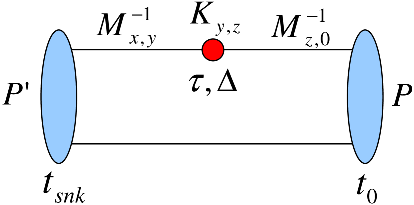
Figure 3: Illustration of a connected contribution to a meson three-point function.

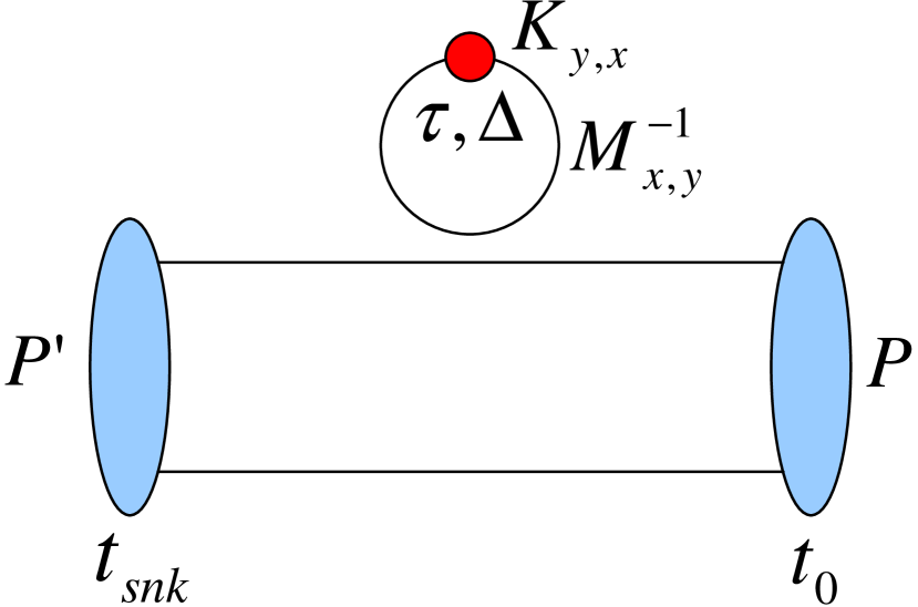
Figure 4: Illustration of a quark line disconnected contribution to a meson three-point function.

Using the $\gamma_{5}$-hermiticity of the fermion matrix, i.e. $\gamma_{5}M\gamma_{5}=(M)^{\dagger}$, translation invariance, $m_{u}=m_{d}$, and setting $\Gamma=\gamma_{5}$ for definiteness, one finds for a pion with momentum $\mathbf{P}$

$$C^{\pi}_{\text{2pt}}(t,\mathbf{P})=\sum_{\mathbf{x}}e^{-i\mathbf{x}\mathbf{P}}\langle\text{Tr}\{M^{-1}_{(\mathbf{x},t);(0,0)}(M^{-1}_{(\mathbf{x},t);(0,0)})^{\dagger}\}\rangle_{U}=\langle G^{\pi}(t,\mathbf{P})\rangle_{U}\,,$$ (121)

i.e. the two-point function (or pion propagator $G^{\pi}(t,\mathbf{P})$) can be readily expressed in terms of the point-to-all quark propagator $M^{-1}_{x,0}$. The corresponding three-point function, Eq. (102), for a $\pi^{+}$ probed by an up-quark operator $\mathcal{O}=\overline{u}K^{\mathcal{O}}u$ can be written as

$$C^{\pi,\mathcal{O}}_{\text{3pt}}(\tau,\mathbf{P}^{\prime},\mathbf{P}) = \sum_{\mathbf{x},y,z}e^{-i\mathbf{x}\mathbf{P}^{\prime}}\langle\text{Tr}\{M^{-1}_{(\mathbf{x},t_{\text{snk}});y}\tilde{K}^{\mathcal{O}}_{y,z}(\tau,\mathbf{\Delta})M^{-1}_{z,0}(M^{-1}_{(\mathbf{x},t_{\text{snk}});0})^{\dagger}\}\rangle_{U}$$ (122)

$$- \langle G^{\pi}(t_{\text{snk}},\mathbf{P}^{\prime})\sum_{y,z}\text{Tr}\{M^{-1}_{z,y}\tilde{K}^{\mathcal{O}}_{y,z}(\tau,\mathbf{\Delta})\}\rangle_{U}\,,$$

which receives contributions from quark-line connected and disconnected parts in the first and the second line, respectively, as illustrated in Figs. 4 and 4. Both quark-line disconnected and connected diagrams involve “point-to-all” and “all-to-all” quark propagators, $M^{-1}_{x,y=0}$ and $M^{-1}_{x,y}$, respectively. While the point-to-all propagators are routinely and efficiently computed by solving sets of linear equations of the type $M_{xz}(M^{-1})_{zy=0}=M_{xz}\phi_{z}=s_{x}$ with source $s$ using, for example, the conjugate gradient method, the inversion of the full Dirac matrix to obtain the all-to-all propagators is prohibitively expensive. Fortunately, for connected diagrams, all-to-all propagators can be completely avoided by using the sequential source technique [MMRT86]. The sequential source technique requires a fixing of the sink interpolating field, in particular the sink time $t_{\text{snk}}$, momentum $\mathbf{P}^{\prime}$, and spin (or the spin-projection). The inconvenient all-to-all propagator in Fig. 4 can then be incorporated into the propagator structure denoted by $\Sigma$ in Fig. 6, called the sequential propagator, which is obtained from $M\gamma_{5}\Sigma^{\dagger}=s^{\prime}$, where the source $s^{\prime}$ itself is written in terms of a point-to-all quark propagator. The advantage of fixing the sink momentum and quantum numbers is that once a set of propagators $M^{-1}_{x,0}$ and sequential propagators $\Sigma$ has been calculated, one is free to study any quark operator $\mathcal{O}$ of interest with some momentum transfer of $\Delta=P^{\prime}-P$ by performing a simple contraction,

$$C^{\pi,\mathcal{O}}_{\text{3pt,con.}}(\tau,\mathbf{P}^{\prime},\mathbf{P})=\sum_{x,y}\big{\langle}\text{Tr}\big{(}\Sigma_{0,x}(t_{\text{snk}},\mathbf{P}^{\prime})\tilde{K}^{\mathcal{O}}_{x,y}(\tau,\mathbf{\Delta})M^{-1}_{y,0}\big{)}\big{\rangle}_{U}\,,$$ (123)

see the illustration in Fig. 6. An alternative to fixing the sink is to construct sequential propagators based on a fixed quark operator $\mathcal{O}$ and momentum transfer $\Delta=P^{\prime}-P$.

Figure 5: Illustration of the sequential source technique.

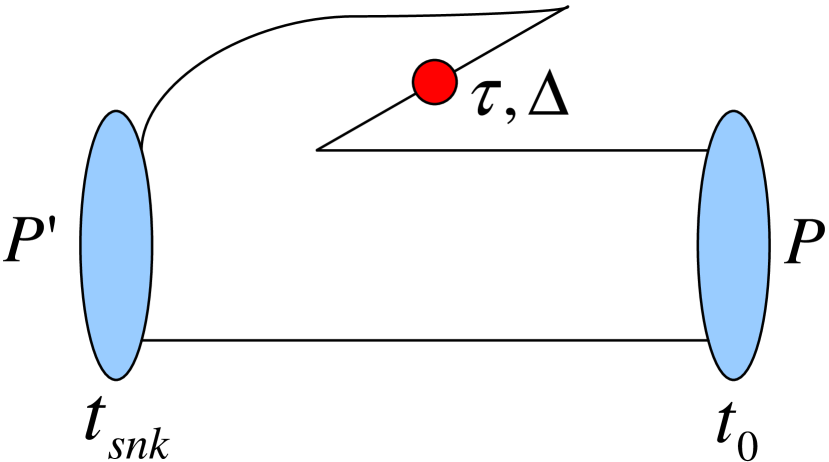
Figure 6: Illustration of anti-quark contributions to a meson three-point function.

We note that the omission of disconnected diagrams, Fig. 4, does not correspond to a calculation in the pure valence quark sector, not even in the quenched approximation. Contributions from anti-quarks can be thought of as already implicitly included in the connected diagrams in the form of so-called “z-graphs”, as illustrated in Fig. 6. Lattice calculations that are based on a finite set of local quark operators therefore do not allow to disentangle contributions from quarks and anti-quarks to observables.

2.3.4 Disconnected diagrams and stochastic methods

Contributions from disconnected diagrams, Fig. 4, which are computationally very expensive due to the unavoidable presence of all-to-all propagators, are often neglected in practical lattice calculations. In the case that the lattice action is isospin symmetric with $m_{u}=m_{d}$, disconnected diagrams cancel out in the isovector channel, i.e. for $\mathcal{O}^{u-d}$. Neglecting disconnected contributions clearly leads to an additional systematic uncertainty for flavor singlet observables. Attempts to compute them are based on stochastic methods. For an introduction to “noise methods”, see, e.g., [Wil99]. First, a set of random noise vectors (or random sources, stochastic sources), for example based on complex $Z(2)$ noise [DL94], $\eta^{(j)}=\pm 1,\pm i$, $(j=1,\ldots,N_{\eta})$, is generated, with the crucial property $N_{\eta}^{-1}\sum_{j}\eta^{(j)}_{x}\eta^{(j)\dagger}_{y}=\delta_{xy}+\mathcal{O}(N_{\eta}^{-1/2})$ (for simplicity, we again suppress Dirac and color indices). The random noise vectors may then be used as random sources in the inversion of $M_{xz}(M^{-1})_{zy=0}=M_{xz}\phi_{z}=\eta^{(j)}_{x}$, which is solved for all $j$ to obtain $\phi^{(j)}$, as in the case of the point-to-all propagators described above. An unbiased estimate of the all-to-all propagator is then given by

$$\frac{1}{N_{\eta}}\sum_{j}\phi^{(j)}_{x}\eta^{(j)\dagger}_{y} = (M^{-1})_{xy}+(M^{-1})_{xz}\left\{\frac{1}{N_{\eta}}\sum_{j}\eta^{(j)}_{z}\eta^{(j)\dagger}_{y}-\delta_{zy}\right\}=(M^{-1})_{xy}+\mathcal{O}(N_{\eta}^{-1/2})\,,$$

showing that the stochastic error of $\mathcal{O}(N_{\eta}^{-1/2})$ is directly related to the (near) off-diagonal elements in $\sum_{j}\eta^{(j)}_{z}\eta^{(j)\dagger}_{y}$. In practice, depending on the number of gauge configurations and stochastic sources and the observable under consideration, the stochastic error can be larger than the usual gauge noise from the Monte Carlo integration. In such cases, a reduction of the stochastic noise is essential. Several noise reduction methods and improvement techniques have been invented and used in practical computations over the years.

The method of “partitioning” [Wil99] or “dilution” [F⁺05] is based on a replacement of each noise vector $\eta^{(j)}$ by a set of new noise vectors $\eta^{(j,p)}$, $p=1,\ldots,N_{p}$, where the $\eta^{(j,p)}$ have zero entries for many color, Dirac and space-time indices. Hence $N_{p}$ times as many inversions are required to get the solution vectors $\phi^{(j,p)}$ for all $j,p$. Assuming that $\eta^{(j)}=\sum_{p}\eta^{(j,p)}$, an estimate of the propagator is then given by $\sum_{j,p}\phi^{(j,p)}_{x}\eta^{(j,p)\dagger}_{y}$, with reduced statistical noise from the off-diagonal contributions. Clearly, the computational overhead due to the larger number of inversions must be taken into account in judging the efficiency of the partitioning.

The truncated eigenmode approach [NEL⁺01] is based on the orthonormal eigensystem of the hermitian fermion matrix $Q\mathbf{v}^{(j)}=\gamma_{5}M\mathbf{v}^{(j)}=\lambda_{j}\mathbf{v}^{(j)}$ and the corresponding spectral decomposition of its inverse,

$$Q^{-1}_{xy}=\sum^{N_{\lambda}}_{j}\frac{1}{\lambda_{j}}\mathbf{v}^{(j)}_{x}\mathbf{v}^{(j)\dagger}_{y}\,.$$ (125)

In the region of small quark masses, the sum will be dominated by the lowest eigenvalues. They can be calculated explicitly, providing a truncated version of the propagator. The remaining subdominant part of $M^{-1}=Q^{-1}\gamma_{5}$ can then be estimated using random noise vectors as described above, reducing the stochastic noise compared to a full stochastic calculation. This approach has been successfully used in, e.g., the calculation of string breaking [BND⁺05], and meson two-point-functions [F⁺05].

Another (perturbative) noise reduction technique, based on the hopping parameter expansion (HPE), is useful in the heavy quark regime and particularly for the (ultralocal) Wilson action [TDLY98]. To briefly introduce this method, we note that the disconnected diagrams as in Fig. 4 are given by correlators of the form $\langle\text{Tr}\{\Gamma M^{-1}\}\times G_{h}\rangle_{U}$, where $G_{h}$ is the hadron propagator, and $\Gamma$ is one of the 16 elements of the Dirac algebra. An unbiased reduction of the noise in the stochastic estimate of the trace can then be achieved by subtracting suitable traceless matrices from $\Gamma M^{-1}$. To this end, the Wilson fermion matrix is written in the form $M=1-\kappa D$ with the lattice Dirac matrix $D$ and the hopping parameter $\kappa=(8r+2m_{q})^{-1}$, see Eqs. (93,94) and related discussion. For large $m_{q}$, the quark propagator can then be expanded in powers of the hopping parameter in a geometric series, $M^{-1}=1+\kappa D+\kappa^{2}D^{2}+\ldots$, which suggest to use $\kappa D,\kappa^{2}D^{2},\ldots$ as a basis to construct the traceless matrices required for the subtraction [TDLY98]. Similar methods based on these ideas, for example the “hopping parameter acceleration”, were already successfully employed in practice [BND⁺05, CBS07, BCS08].

2.3.5 “One-end-trick”

Stochastic sources, $\eta^{(j)}$, are not only an essential tool for the evaluation of disconnected diagrams, but can also be very useful in the calculation of connected contributions to hadron correlators, using the so-called “one-end-trick” [FM99]. For the two-point function Eq. (121) for the pion, $\Gamma=\gamma_{5}$, a stochastic source $\eta^{(j)}_{(\mathbf{x},t)}=\eta^{(j)}_{(\mathbf{x})}\delta_{t,t_{0}}$, with the corresponding solution vector (see section above)

$$\phi^{(j)}_{(\mathbf{x},t);t_{0}}=\sum_{\mathbf{z}}(M^{-1})_{(\mathbf{x},t);(\mathbf{z},t_{0})}\eta^{(j)}_{(\mathbf{z},t_{0})}\,,$$ (126)

is sufficient to give an unbiased estimate of the form

$$\sum_{\mathbf{x}}\langle\text{Tr}\{\sum_{j}^{N_{\eta}}\phi^{(j)}_{(\vec{x},t);t_{0}}\phi^{(j)\dagger}_{(\vec{x},t);t_{0}}\}\rangle_{U} \approx \frac{1}{V}\sum_{\mathbf{x},\mathbf{y}}\langle\text{Tr}\{M^{-1}_{(\mathbf{x},t);(\mathbf{y},t_{0})}(M^{-1}_{(\mathbf{x},t);(\mathbf{y},t_{0})})^{\dagger}\}\rangle_{U}=C^{\pi}_{\text{2pt}}(t,\mathbf{P})\,,$$ (127)

with a stochastic error of $\mathcal{O}(N_{\eta}^{-1/2})$. Compared to Eq. 121, one finds that the estimate with stochastic sources leads to an additional volume average, $V^{-1}\sum_{\mathbf{y}}$, and therefore potentially a dramatic increase in statistics. The reason is that the summation over the source position $\mathbf{y}$ is already implicit in the stochastic average. This has been numerically studied and also extended to other mesons and for the calculation of three- and four-point functions in hadron structure calculations [Sim07, BJKK08, AK08, B⁺08e], where in many cases a substantial increase in statistics was found at fixed cost for the pion using stochastic sources compared to conventional point sources. Some recent applications will be discussed in more detail in sections 3.3 and 6.0.1 below.

2.3.6 Partially twisted boundary conditions

Many of the fundamental hadron structure observables that were introduced and discussed in section 2.1 above are defined at vanishing momentum transfer squared, $t=0$ or $q^{2}=-Q^{2}=0$. Typical examples are mean square radii, Eq. (60), the anomalous magnetic moment of the nucleon, $\kappa=F_{2}(Q^{2}=0)$, the quadrupole moment of the $\rho$-meson, $Q_{\rho}=G_{Q}(Q^{2}=0)/m_{\rho}^{2}$, and angular momentum contributions to the nucleon spin, Eq. (70), $J=(A_{20}(t\text{{=}}0)+B_{20}(t\text{{=}}0))/2$. The numerical analysis of these quantities requires, however, small non-zero values of the momentum transfer $q=\Delta=P^{\prime}-P$: Derivatives in the definition of charge radii have to be approximated by finite differences, and the other relevant form factors and generalized form factors are multiplied by factors of $\Delta$ in the parametrization of the respective hadron matrix elements, cf. Eqs. (9,20,21,22,41,42,66,…), and therefore cannot be extracted in the forward limit, $P^{\prime}=P$. As already noted in section 2.3.1, periodic boundary conditions are conventionally used in spatial directions for the discretized fields, leading to discrete momenta of the form $\mathbf{P}=(2\pi/(aL))\mathbf{n}$. The analysis of the observables mentioned above is therefore challenging in current lattice simulations, where lattice spacings $a$ and spatial extents $L$ are such that the lowest non-zero momentum components are $P\gtrapprox 0.3\text{ GeV}$, resulting in comparatively large non-zero momentum transfers of $|t|^{\not=0}\gtrsim 0.15-0.4\text{ GeV}^{2}$. Furthermore, because of the discrete lattice momenta, neighboring values of $t$ are often separated by large gaps of up to $\approx 0.5\text{ GeV}^{2}$. The interpolation between accessible values of the momentum transfer, and the extrapolation to the forward limit therefore requires in general a parametrization of the ($t$-) $Q^{2}$-dependence of the (generalized) form factors based on a certain ansatz, e.g., a monopole or dipole, which introduces additional systematic uncertainties. These difficulties may be avoided to some extent by using so-called partially twisted boundary conditions (pTBCs) [SV05, BC05] in spatial directions. The advantage of pTBCs over (fully) twisted BCs is that they are only applied to the valence quark fields in the quark propagators, while the sea quarks obey the conventional periodic BCs. Hence existing dynamical gauge configurations generated using periodic BCs may be employed for the calculation of correlators. The price one has to pay is the appearance of additional finite volume effects, see below.

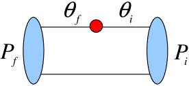
Figure 7: Illustration of pTBCs.

As illustrated in Fig. 7, pTBCs are of the form

$$q_{f,i}(\mathbf{x}+aL\hat{\mathbf{e}}_{j})=e^{i(\boldsymbol{\theta}_{f,i})_{j}}q_{f,i}(\mathbf{x})\,$$

with twisting angles $(\boldsymbol{\theta}_{f,i})_{j}=0,\ldots,2\pi$, $j=1,2,3$, for the ‘final’ and and ‘initial’ valence quark fields. Denoting the conventional discrete (‘Fourier’) momenta by $\mathbf{P}^{F}_{f,i}=(2\pi/(aL))\mathbf{n}_{f,i}$, and setting $\mathbf{P}^{\text{pTBC}}_{f,i}=\mathbf{P}^{F}_{f,i}+\boldsymbol{\theta}_{f,i}/(aL)$, the squared momentum transfer for twisted BCs is given by

$$t=\big{(}E(\mathbf{P}^{\text{pTBC}}_{f})-E(\mathbf{P}^{\text{pTBC}}_{i})\big{)}^{2}-\big{(}\mathbf{P}^{\text{pTBC}}_{f}-\mathbf{P}^{\text{pTBC}}_{i}\big{)}^{2}\,,$$

where as usual $E(\mathbf{P})^{2}=m^{2}+\mathbf{P}^{2}$. Clearly, setting the conventional discrete (‘Fourier’) momenta equal to zero, $\mathbf{n}_{f,i}=0$, and tuning the twisting angles $\boldsymbol{\theta}_{f,i}$, arbitrarily small values of the momenta and thereby the momentum transfer can be accessed. Non-zero Fourier momenta and twisting angles can also be combined to reach larger fine-tuned values of $t$ allowing to, e.g., fill the gaps between the $t$-values that are accessible with periodic BCs. Partially twisted BCs can be implemented in practice by replacing the pTBC quark fields by new quark fields, $\tilde{q}(x)$, which obey periodic BCs, $q(x)=\exp(i\boldsymbol{\theta}\cdot\mathbf{x}/L)\tilde{q}(x)$. Since this can be seen as gauge transformation, in order to implement pTBCs, effectively only the link variables in the propagators have to be replaced, $U_{x,x+a\hat{\mathbf{e}}_{j}}\rightarrow\exp(i\boldsymbol{\theta}_{j}a/L)U_{x,x+a\hat{\mathbf{e}}_{j}}$ [FJS06].

Finite volume effects (FVEs) due to pTBCs were shown to be in general exponentially suppressed in the volume [SV05, BC05], i.e. $\propto\e^{-m_{\pi}L}$. Detailed studies [JT07, JT08c] in partially quenched chiral perturbation theory (pQChPT), see following section, showed that they can indeed expected to be small in current lattice calculations of the pion form factor, and that isospin symmetry breaking effects in particular can be avoided by working in the Breit frame, i.e. choosing $\boldsymbol{\theta}_{f}=-\boldsymbol{\theta}_{i}$. Similar investigations in the nucleon sector showed that the FVEs from pTBCs are small, of the order of a few percent, for the isovector electric form factor [Tib06], but can be as large as $\approx 20\%$ in the case of the magnetic or Pauli form factor [Tib06, JT08a], for small twisting angles and typical parameters of current lattice simulations. This has to be kept in mind regarding the preliminary lattice results for $F_{2}^{u-d}$ obtained with pTBCs that will be discussed below in section 6.0.4. Some applications of pTBC in meson structure calculations will be presented in sections 3.3.

2.4 Chiral effective field theory and chiral perturbation theory

Due to the substantial progress in lattice QCD simulations over the last couple of years, the lowest pion masses that can be reached in hadron structure investigations today are $\sim 300$ MeV in physical volumes of $\sim(3\mbox{fm})^{3}$, with lattice spacings $\sim 0.1$ fm. Clearly, to exploit the lattice results as much as possible, extrapolations to the infinite volume limit, the continuum limit, and to the physical pion mass are necessary. In order not to spoil the “ab-initio”-character of lattice QCD calculations, such extrapolations must be addressed in a systematic way. This is in general possible using the methods of low energy effective field theories (EFT), based on a systematic expansion in powers $p/\Lambda$, where $p$ generically denotes a small mass, energy or momentum, and where $\Lambda$ is a “large” energy scale. In massless QCD, the chiral $SU(3)_{L}\times SU(3)_{R}$ (where $SU(3)_{L/R}$ acts on the left and right handed $u$, $d$, and $s$ quark fields, respectively) symmetry is spontaneously broken at the fundamental chiral symmetry breaking scale $\Lambda_{\chi}$, giving rise to eight Goldstone bosons. The Goldstone bosons can be identified with the pions, kaons and the eta, and to leading order in $p/\Lambda$, the low energy EFT of QCD can be uniquely formulated in terms of these degrees of freedom. One often identifies $\Lambda^{2}_{\chi}=(4\pi f^{0}_{\pi})^{2}\approx 1\text{ GeV}^{2}$, where $f^{0}_{\pi}\simeq 0.09\text{ GeV}$ is the pion decay constant in the chiral limit. An alternative is to set the chiral symmetry breaking scale equal to the mass of the lowest lying non-Goldstone meson, i.e. the $\rho$-meson. The low energy EFT of QCD is, strictly speaking, non-renormalizable, and an increasing number of couplings or low energy constants (LECs), in addition to $f^{0}_{\pi}$, are required at higher orders to permit a systematic order-by-order renormalization. The a priori unknown LECs thereby parametrize part of the physics of the underlying full theory that is not directly accessible within the low energy EFT. The predictive power of the EFT-approach is due the fact that the LECs are universal and process independent.

Terms providing an explicit chiral symmetry breaking at non-zero quark masses can be included in the EFT in a perturbative way, giving rise to non-vanishing pseudoscalar meson masses. The meson masses are related to the quark masses in a non-trivial manner, described by the Gell-Mann-Oakes-Renner (GMOR) relation at leading order,

$$m_{\pi}^{2}=-\frac{1}{(f^{0}_{\pi})^{2}}\langle\overline{\psi}\psi\rangle\overline{m}+\mathcal{O}(p/\Lambda_{\chi})\,$$ (128)

where $\langle\overline{\psi}\psi\rangle=\langle(\overline{u}u+\overline{d}d)\rangle$ is the quark condensate, and $\overline{m}=(m_{u}+m_{d})/2$. Similar relations hold for the kaons and the $\eta$-meson. A power counting scheme has been developed that allows for a systematic expansion in $p/\Lambda_{\chi}$ to all orders, where pion loop diagrams are suppressed by $(p/\Lambda_{\chi})^{2}$ relative to the tree level contributions [GL84]. Such a perturbative expansion is called chiral perturbation theory (ChPT) and predicts in particular the form of the quark mass dependence (or pion mass dependence using Eq.(128)) of, e.g., pseudoscalar meson masses, decay constants, form factors, etc. Apart from the analytic quark mass dependence in terms of powers of $m_{\pi}^{2}$, pion loop diagrams in ChPT lead to the famous (“non-analytic”) chiral logarithms, $m_{\pi}^{2}/(4\pi f^{0}_{\pi})^{2}\ln(m_{\pi}^{2}/\lambda^{2})$. Here, we have included a factor $(4\pi)^{2}$ that is characteristic for the loop integration, and $\lambda$ is the renormalization scale. An illustration of contributions to the pion form factor at leading order ($\mathcal{O}(p^{2})$) and 1-loop ($\mathcal{O}(p^{4})$) level is given in Fig. 8.

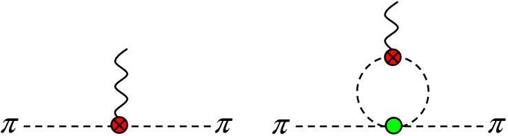
Figure 8: Illustration of contributions to the pion form factor in ChPT. The coupling to the external vector current is denoted by the crossed circle.

References to meson structure observables that have been studied in ChPT will be given at the beginnings of sections 3 and 4.

The inclusion of baryons DOFs into the low energy EFT is formally straightforward, but leads to conflicts within the simple power counting scheme used in the pure mesonic sector, since baryon momenta in the full relativistic theory are generically large, $p_{B}\simeq m_{B}\simeq\Lambda_{\chi}$. The power counting scheme can be saved by treating the baryons as heavy particles and employing a non-relativistic expansion in $p/m_{B}$, where $p=p_{B},p_{\pi},m_{\pi},\ldots$ [JM91]. The result of such a procedure, which can formally be carried out to any order, is called heavy baryon ChPT (HBChPT). For an early review we refer to [BKM95]. In HBChPT, higher resonances are usually integrated out and consistently included in an implicit way in the form of counter-term contributions. It has however been noted early on that the $\Delta(1232)$ resonance is special in at least two ways. First, the nucleon-$\Delta$ mass splitting is less than two times the pion mass and therefore does not qualify easily as a large scale, and at the same time the pion-nucleon-$\Delta$ coupling constant is phenomenologically large. Based on these observations, a formalism called small scale expansion (SSE) was developed to consistently include explicit $\Delta(1232)$ degrees of freedom into the HBChPT formalism [HHK97b]. Within the SSE, the mass splitting $\text{{\small$\Delta$}}m_{N\Delta}\approx 0.27\text{ GeV}$ is treated on the same level as the pion mass, momentum, etc. as small parameter $\epsilon=\text{{\small$\Delta$}}m_{N\Delta},p_{\pi},m_{\pi},\ldots$ We note that a number of nucleon structure calculations have been performed in a somewhat modified version of the HBChPT-SSE developed in [HW02] and further pursued in, e.g., studies of the nucleon mass and of $g_{A}$ in [PMW⁺06] and [PMHW07], respectively. Another method including explicit $\Delta$-DOFs, called $\delta$-expansion scheme, where the small expansion parameter is $\delta=\Delta/\Lambda_{\chi}\sim m_{\pi}/\Delta$, implying that $\delta^{2}\sim m_{\pi}$, has been developed in [PP03] and, e.g., employed in a relativistic (see below) ChPT-study of the magnetic moment of the $\Delta$-baryon [PV05].

For many years, due to the lack of a consistent relativistic formulation, hadron structure observables have been mostly investigated in the HBChPT (and the SSE, $\delta$-expansion) formalism. This is slowly changing since Becher and Leutwyler [BL99] developed a consistent power counting scheme including baryons based on the so-called infrared regularization (IR) of loop integrals. This has been employed for example already in [KM01] in a slightly modified form for the analysis of the nucleon electromagnetic form factors. Since then, further covariant renormalization schemes like the extended on-mass shell (EOMS) [SGS04] and the modified IR ($\overline{\text{IR}}$) [DGH08] schemes have been developed, so that today solid alternatives to the HBChPT approach are available. An approach alternative to the usual dimensional regularization of loop integrals is based on a finite-range regularization (FRR) [DHB99, YLT03, LTY04].

To this day, a large number of baryon structure observables have been studied in covariant and heavy BChPT, for example nucleon form factors, including charge radii, magnetic moments and the axial vector coupling constant, moments of polarized and unpolarized nucleon PDFs and GPDs, including in particular the form factors of the QCD energy momentum tensor nucleon polarizabilities, etc. For a recent review of the investigation of baryons in ChPT we refer to [Ber08].

Depending on the order of the chiral expansion, the pion mass dependence of a given hadronic matrix element depends in general on several a priori unknown LECs. One can envisage at least two different scenarios:

• In the rare case that all relevant LECs can be determined from experiment and phenomenology, ChPT gives a parameter-free prediction of the pion mass dependence of the observable under consideration to a given order, which can be directly compared to results from lattice QCD.

• In the general case, the numerical values of (some of) the LECs are unknown. The unknown LECs may be then be obtained from a fit of the full ChPT result to lattice simulation data at different $m_{\pi}$ and results from experiment at the physical pion mass (if available). Alternatively, one may want to fit to lattice data points alone in order to be able to ‘predict’ (a priori or a posteriori) the value at the physical point.

In either case, it is of crucial importance to study the convergence of the ChPT series, and to avoid stretching the chiral extrapolation beyond its region of applicability. These are difficult tasks in praxis since most of the lattice hadron structure results are available only for pion masses larger than $300$ MeV. The region of applicability of ChPT is being studied intensively and will certainly depend to some extent on the calculational scheme, e.g. HBChPT compared to covariant BChPT, as well as the observables under consideration. On the lattice side, one has to keep in mind that in most cases finite volume and discretization effects are not perfectly under control, so that an extrapolation in the pion mass alone based on infinite volume, continuum ChPT is subject to systematic uncertainties of largely unknown size. At this point, it should be stressed that ChPT not only predicts the form of the pion mass dependence of hadronic observables, but can also be extended to include finite volume effects as well as corrections at non-zero lattice spacing (discretization effects). Chiral perturbation theory calculations in a finite volume have already been carried out for different hadron structure observables. An interesting example is the axial-vector coupling constant $g_{A}$ that was studied in HBChPT in finite volume in [BS04, K⁺06, PMHW07]. Discretization effects for different (mixed) lattice actions have been investigated in particular for hadron masses and decay constants (see, e.g., [BRS04, BBRS05]) and also for nucleon magnetic moments [BS03].

Chiral perturbation theory calculations at higher orders, including finite volume and discretization effects, are certainly desirable. However, one has to keep in mind that the number of unknown LECs increases with the order of the ChPT calculation.

References to results from ChPT for the structure of mesons and baryons in terms of form factors and moments of PDFs and GPDs will be given at the beginnings of the corresponding sections below.

3 Lattice results on form factors

3.1 Overview of lattice results

Here we briefly summarize the current standing of each of the topics that will be discussed in more detail later in this section.

First lattice calculations in the quenched approximation of the pion electromagnetic form factor, $F_{\pi}(Q^{2})$, have been published already in the late 1980’s [MS88, DWWL89]. Since then, further quenched and unquenched lattice results for $F_{\pi}(Q^{2})$ have been been presented [vdHKL04, BEF⁺05, H⁺06], and an extensive study in unquenched lattice QCD has more recently been published in [B⁺07f]. Up-to-date calculations in unquenched lattice QCD employing for example partially twisted boundary conditions (pTBCs) to access $F_{\pi}(Q^{2})$ at very low non-zero $Q^{2}$ and all-to-all propagators (see end of previous section 2.3.3) can be found in [Sim07, BFJ⁺07, B⁺08e, J⁺08, FLS09]. First results for the tensor form factor of the pion, $B^{\pi}_{T10}$, have been published in [B⁺08h].

A first lattice calculation of the electric form factor of the proton in quenched QCD was published in 1989 [MS89]. Since then, several quenched lattice QCD studies of the nucleon electromagnetic form factors, including charge radii and magnetic moments, appeared [DWL90, LWD91, WDL92, G⁺05e, BLW⁺06]. Interestingly, to this date, there is only a small number of peer-reviewed publications on the electromagnetic form factors of the nucleon in unquenched lattice QCD available [AKNT06, LBO⁺08]. A larger number of unquenched results can be found in proceedings [N⁺04, R⁺05, E⁺05, E⁺06b, G⁺06c, G⁺07a, G⁺07b, OY08, B⁺08f]. For an overview and a discussion of nucleon electromagnetic form factors in lattice QCD we also refer to [ARZ07].

Early studies of the axial vector form factors, $G_{A}(Q^{2})$ and $G_{P}(Q^{2})$, of the nucleon in quenched QCD have been presented in [LDD⁺94, LDDW95], and more recent results in unquenched lattice QCD can be found in [AKL⁺07, LBO⁺08].

The nucleon isovector axial vector coupling constant $g_{A}=G_{A}(Q^{2}=0)$ was studied quite intensively in recent years. A detailed quenched study based on chiral (domain wall) fermions can be found in [SOOB03], and dynamical lattice results have been published in [K⁺06, E⁺06a, Y⁺08]. Unquenched calculations of the isosinglet axial vector coupling constant have been presented in [FKOU95, DLL95, G⁺99b], including estimates of contributions from disconnected diagrams.

The nucleon tensor charge, $g_{T}$, has been investigated in quenched QCD for the first time in [ADHK97] and later using domain wall fermions in [OBO06]. More recent results for $g_{T}$ in full QCD can be found in [D⁺02, G⁺05g, E⁺06b, LBO⁺08]. First unquenched lattice QCD calculations of the nucleon tensor form factors $g_{T}(Q^{2}=-t)=A_{T10}(t)$, $B_{T10}(t)$ and $\tilde{A}_{T10}(t)$ have been presented in [G⁺05g, G⁺07d].

A first direct lattice calculation of $\rho$-meson vector form factors, $G_{C}(Q^{2})$, $G_{M}(Q^{2})$ and $G_{Q}(Q^{2})$, in quenched QCD was published recently [H⁺07b] (restricted to $Q^{2}=0$ and a single non-zero momentum transfer, $Q^{2}\simeq 0.1$ GeV²). A short while ago, preliminary results for $G_{C}(Q^{2})$, $G_{M}(Q^{2})$ and $G_{Q}(Q^{2})$ for a range of values of $Q^{2}$ were obtained in full lattice QCD [G⁺08d]. Related results based on density-density correlators in quenched and unquenched lattice QCD can be found in [AdFT03, AK07, AK08].

The electromagnetic form factors of the decuplet baryons, including their quadrupole and octupole moments, have been studied already some time ago in quenched lattice QCD based on results for $Q^{2}=0$ and a single non-zero momentum transfer $Q^{2}\sim 0.1\text{ GeV}^{2}$ [LDW92] and more recently for $Q^{2}\sim 0.23\text{ GeV}^{2}$ in [B⁺09c]. A more detailed analysis of the $Q^{2}$-dependence of the electromagnetic form factors of the $\Delta$-baryon in quenched and unquenched lattice QCD has been performed recently [A⁺09a].

Selected results from mostly from unquenched (including hybrid) lattice QCD simulations will be discussed in some detail below.

3.2 Results from chiral perturbation theory

Pion

The $m_{\pi}$- and $Q^{2}$-dependence of the pion vector form factor in infinite volume has already been calculated 25 years ago at 1-loop level in ChPT in the seminal paper by Gasser and Leutwyler [GL84] (see also [GL85]). A finite volume study of $F_{\pi}(Q^{2})$ to $\mathcal{O}(p^{4})$ using lattice regularized ChPT was carried out in [BL05]. Results for the pion form factor in the framework of partially-quenched ChPT (PQChPT) at one-loop order in a finite volume, including the lattice spacing dependence for a mixed-action theory of Ginsparg-Wilson valence quarks and staggered sea quarks were obtained in [BJT06]. By now, many observables in the mesonic sector have also been studied at NNLO ($\mathcal{O}(p^{6})$), including 2-loop diagrams. An overview can be found in [Bij07]. Particularly relevant for the structure of the pion is the pion mass dependence of $F_{\pi}(Q^{2})$ at 2-loops in infinite volume ChPT [GM91, BCT98]. First results for the pion mass and $Q^{2}$-dependence of the tensor (chiral-odd ) form factor of the pion, $B^{\pi}_{T10}(Q^{2})$, were obtained in [DMS07] at leading 1-loop level in ChPT. Results for the pion vector and tensor form factor in a finite volume in the framework of PQChPT became available soon thereafter [CDS07]. Furthermore, due to the reduced space-time symmetries on the lattice, the off-forward pion matrix elements of the vector current and the tensor operator receive finite volume corrections in form of additional kinematical structures and calculable “form factors”, which have been worked out in [MS07]. Finite volume effects introduced by partially twisted boundary conditions are in general exponentially suppressed [BC05, SV05]. Although probably small in current dynamical calculations of the pion form factor, they may be non-negligible in future lattice calculations at pion masses $m_{\pi}<300\text{ MeV}$ and for not too large volumes, as has been worked out in PQChPT to NLO in [JT07] for rest frame kinematics, where both isospin and hypercubic symmetry breaking effects are present. More recently, these calculations have been revisited in the Breit frame, where isospin and a discrete rotational symmetry are preserved [JT08c].

Nucleon

As explained in section 2.4, a direct implementation of baryons, in particular the nucleon, into the relativistic EFT framework leads to a conflict with the standard ChPT-expansion due to lack of a consistent power counting scheme. This has been overcome in the heavy baryon ChPT (HBChPT) formalism, which has been used in practice from the early 1990’s on. The isovector Dirac and Pauli form factors of the nucleon were studied at 1-loop level ($\mathcal{O}(p^{4})$) in SU(2) HBChPT in [BKKM92], and further activities in this framework during the early years have been reviewed in [BKM95], including results for the nucleon axial-vector form factor $G_{A}(Q^{2})$ and the pseudo-scalar form factor $G_{P}(Q^{2})$. Systematically taking into account explicit $\Delta$-baryon degrees-of-freedom in the chiral expansion, the isovector nucleon form factors $G_{E,M}(Q^{2})$ and $F_{1,2}(Q^{2})$ were revisited in the framework of the small scale expansion (SSE) (see section 2.4) in [BFHM98]. Based on a modified chiral power counting of the isovector $\Delta$-nucleon transition coupling constant $c_{V}$, a calculation of the nucleon isovector anomalous magnetic moment $\kappa$ to NLO ($\mathcal{O}(\epsilon^{3})$) in the framework of a revised version of the SSE HBChPT formalism was presented in [HW02]. These calculations were extended later [G⁺05e] to include the full $Q^{2}$-dependence of the isovector nucleon form factors, $F_{1,2}(Q^{2})$, at NLO in SSE HBChPT. Employing a consistent power counting scheme based on infrared-regularization ($IR$) [BL99], the nucleon vector form factors have been investigated in relativistic baryon ChPT (BChPT) in [KM01], where explicit results for the pion mass dependence of the isovector and isoscalar anomalous magnetic moments and the charge radii of $G_{E,M}(Q^{2})$ can be found. Nucleon electromagnetic form factors were also studied in relativistic BChPT in [FGS04] employing the extended on-mass-shell renormalization scheme. In [WLTY07] and [WLTY08], chiral extrapolations of the nucleon magnetic form factors and octet-baryon charge radii, respectively, have been studied using finite-range regularization.

A detailed study of the nucleon axial vector coupling constant $g_{A}$ in the SSE approach to $\mathcal{O}(\epsilon^{3})$ has been presented in [HPW03]. The lattice spacing dependence at $\mathcal{O}(a)$ of $g_{A}$, for Wilson fermions and a mixed formulation of Wilson sea and Ginsparg-Wilson valence fermions, has been studied in the framework of PQChPT including explicit $\Delta$-DOFs in [BS03]. In a work by the same authors [BS04], the leading finite volume corrections to $g_{A}$ have been obtained in HBChPT including explicit $\Delta$-DOFs, in a framework that differs somewhat from the SSE formalism mentioned above. Subsequently, the SSE calculation of [HPW03] was extended to include finite volume corrections and applied to unquenched lattice QCD results in [K⁺06]. In addition, a matching and comparison of the employed SSE-LECs to the LECs used in [BS04] was attempted. Results for the axial vector and pseudoscalar form factors, including the axial vector coupling constant, have also been obtained in relativistic BChPT to $\mathcal{O}(p^{4})$ [SFGS07]. Due to the reformulated IR-scheme employed in this work, it was also possible to include the axial vector meson $a_{1}$ explicitly as an additional DOF in the chiral expansion. The specific form of $g_{A}$ at 2-loop level in HBChPT has been worked out in [BM06], where also the coefficient of the double logarithmic term, as well as several other numerically important contributions, were obtained. More recently, lattice spacing artifacts for the nucleon matrix element of the axial vector current have been investigated to $\mathcal{O}(a^{2})$, for a mixed action approach of Ginsparg-Wilson and staggered sea quarks, in PQChPT with explicit $\Delta$ DOFs [Jia07].

The leading chiral logarithmic contributions in HBChPT to the nucleon tensor charge can be be found in [AS02, CJ01], and in [DMS07], the full set of nucleon tensor form factors have been studied in HBChPT at leading 1-loop level. A broad study of baryon matrix elements of twist-2 operators including vector, axial vector and tensor currents in the framework of (partially quenched) HBChPT at finite and infinite volume has been presented in [DL05].

Delta

The leading non-analytic contributions in HBChPT to the magnetic and quadrupole moments of the decuplet baryons, including the $\Delta$ resonance, were studied for the first time in [BSS94], however no explicit expressions for the pion mass dependences of $\mu_{\Delta}$ and $Q_{\Delta}$ are given in this work. More explicit results are given in [BM96], where the HBChPT calculation of the decuplet magnetic moments has been revisited, differing from [BSS94] by the inclusion of the Roper resonance as intermediate state, and in the treatment of $SU(3)$ flavor symmetry. On the basis of the $\delta$-expansion scheme detailed in [PP03], the $m_{\pi}$-dependence of the magnetic moment of the $\Delta$-baryon has been calculated in a covariant way to NLO [PV05]. A study of the magnetic moment of the $\Delta$-baryon using the extended on-mass-shell renormalization scheme in relativistic BChPT has been presented in [HWGS06].

Recently, the pion mass dependence of the axial vector coupling constant of the $\Delta$-baryon has been studied in full and partially quenched HBChPT to NLO [JT08b], where also isospin relations for the underlying $\Delta$-matrix elements of the axial vector current were derived, which could serve as a useful guide for future lattice calculations of this observable.

Charge radii, magnetic and quadrupole moments of decuplet baryons, with particular emphasis on a separation of connected and disconnected contributions, were investigated recently in [Tib09] using partially quenched ChPT.

Polarizabilities

The Compton scattering amplitude for the nucleon, parametrized by the nucleon electric, magnetic and spin polarizabilities, has been studied at length over the years in ChPT. For an overview, we refer to the review [Ber08] and the extensive studies in [HGHP04, BMM⁺05, DTWL06]. The spin-independent nucleon polarizabilities, cf. section 2.1.10, Eq. (83), were studied first in [BKM91, BKM92] in HBChPT at leading 1-loop level (to $\mathcal{O}(q^{3})$). In [BKSM93], this calculation was extended to $\mathcal{O}(q^{4})$. Contributions from kaons and baryon resonances as intermediate states were studied in [BS92] at leading order in the heavy baryon limit. A calculation of the polarizabilities in the SSE scheme to $\mathcal{O}(\epsilon^{3})$ including explicit $\Delta$-baryon intermediate states was presented in [HHK97a], and a similar study in the $\delta$-expansion scheme, also including explicit $\Delta$-DOFs, can be found in [PP03]. More recently, the volume dependence of the polarizabilities has been studied in the framework of HBChPT [DTWL06], where also results for (partially) quenched QCD are provided.

3.3 Pion form factors

Instead of going in detail through the history of lattice QCD calculations of the pion electromagnetic form factor, we will concentrate here on recent results for $F_{\pi}$ obtained in unquenched lattice simulations. To begin with, we show in Fig. 10 an overview plot of $F_{\pi}(Q^{2})$ as a function of $Q^{2}$, including experimental data points and (chirally extrapolated, see below) lattice QCD results from QCDSF-UKQCD for $n_{f}=2$ flavors of improved Wilson fermions and Wilson glue [B⁺07f]. The large number of lattice data points have been obtained on the basis of 15 ensembles with pion masses ranging from $400$ to $1200\text{ MeV}$ and for lattice spacings in the range $a\sim 0.07,\ldots,0.12\text{ fm}$. Since the local (non-conserved) vector current has been used, the bare lattice data has been renormalized to ensure charge conservation, i.e. such that $F_{\pi}(Q^{2}=0)=1$. A monopole ansatz

$$F_{\pi}(Q^{2},m_{\pi}^{2})=\frac{F_{\pi}(0)}{1+\frac{Q^{2}}{m_{\text{mono}}^{2}(m_{\pi}^{2})}}\,,$$ (129)

with $F_{\pi}(0)=1$ and $m_{\text{mono}}^{2}(m_{\pi}^{2})=c_{0}+c_{1}m_{\pi}^{2}$ was fitted to the lattice data to simultaneously parametrize the $Q^{2}$- and $m_{\pi}^{2}$-dependence. On the basis of this fit, the lattice results have been shifted to the physical point by subtracting the difference $F_{\pi}(Q^{2},(m^{\text{lat}}_{\pi})^{2})-F_{\pi}(Q^{2},(m^{\text{phys}}_{\pi})^{2})$ from the individual data points. The shifted data points are shown in Fig. 10, and turn out to be in very good agreement with the experimental results over the full range of $Q^{2}=0,\ldots,4.4\text{ GeV}^{2}$, and in particular at small $Q^{2}$ as displayed in the inset in the upper right corner of Fig. 10. Notwithstanding the overall successful description of the lattice results based on Eq. 129, it is important to explicitly study the pion mass dependence of the monopole masses, as obtained from separate monopole fits at fixed $m_{\pi}$. This can be done on the basis of Fig. 10, displaying $m_{\text{mono}}^{2}$ as a function of $m_{\pi}^{2}$. Comparing different ansätze for the pion mass dependence of $m_{\text{mono}}$, it was shown that the form $m_{\text{mono}}^{2}(m_{\pi}^{2})=c_{0}+c_{1}m_{\pi}^{2}$ that has been used in the global fit above provides the best description of the lattice data in terms of $\chi^{2}/\text{DOF}$. The resulting chiral extrapolation, represented by the shaded band in Fig 10, gives a value of $m_{\text{mono}}=0.727\pm 0.016_{\text{stat}}+0.024_{\text{vol}}\pm 0.046_{\text{sys}}\text{ GeV}$ at the physical pion mass, where also estimates of uncertainties due to finite volume effects (vol) and the fit- and chiral-extrapolation ansatz (sys) have been included. This corresponds to a mean square charge radius of $\langle r_{\pi}^{2}\rangle=6/m_{\text{mono}}^{2}=0.441\pm 0.019_{\text{stat}}-0.029_{\text{vol}}\pm 0.056_{\text{sys}}\text{ fm}^{2}$, which is in good agreement with the experimental value of $\langle r_{\pi}^{2}\rangle=0.451(11)\text{ fm}^{2}$ from the PDG [A⁺08i]. Since most of the lattice data points in Fig. 10 correspond to rather large pion masses of $m_{\pi}>590\text{ MeV}$, and since the only data point with $m_{\pi}=400\text{ MeV}$ has little statistical weight, a theory-based chiral extrapolation employing results from ChPT discussed in the previous section has not been attempted in this case.

Figure 9: Pion electromagnetic form factor $F_{\pi}$ in lattice QCD (horizontal dashes) and experiment (diamonds) (from [B⁺07f]).

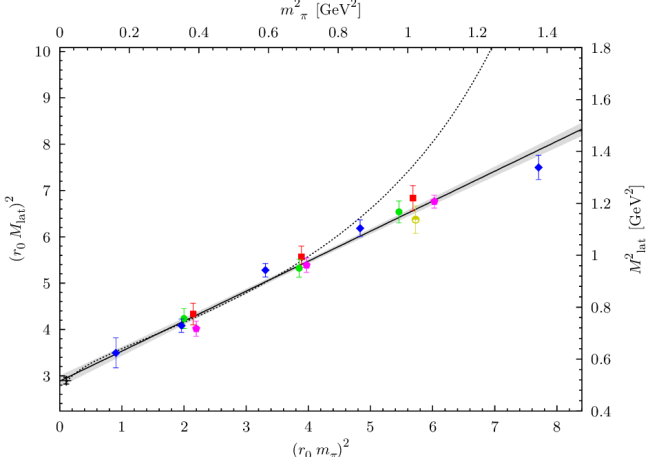
Figure 10: Chiral extrapolation of the monopole mass (from [B⁺07f]).

Recently, RBC-UKQCD calculated the pion form factor for a pion mass of $m_{\pi}=330\text{ MeV}$, employing partially twisted boundary conditions, as explained at the end of section 2.3.3 above, to reach very low non-zero values of $Q^{2}$ [B⁺08e]. The calculation is based on a simulation with $n_{f}=2+1$ flavors of domain wall fermions and the Iwasaki gauge action, for a single lattice spacing of $a\approx 0.114\text{ fm}$ in a volume of $V\approx(2.74\text{ fm})^{3}$. In contrast to traditional point sources, random wall (or noise-) sources with $Z(2)$ noise on a single color- and spin-index combination have been used for the inversion of the Dirac matrix. For this particular calculation, it was shown that a reduction of the computational cost by a factor of $\approx 12$ could be achieved compared to a conventional point source computation with the similar statistical precision. In combination with twisted boundary conditions for the valence quarks (pTBCs), high precision results were obtained for the pion form factor at very small, non-zero values of the momentum transfer squared, $Q^{2}=0.013,0.022$ and $0.035\text{ GeV}^{2}$, as displayed in Fig. 12. Quite remarkably, the lowest $Q^{2}$ accessed in the lattice calculation is even below the lowest $Q^{2}$ reached by experiment, and the statistical errors of the two leftmost lattice data points in Fig. 12 are smaller than for the experimental data points. Owing to the very low $Q^{2}$ that could be accessed, and the reasonably low pion mass of $330\text{ MeV}$, a fit to results from $SU(2)$ ChPT at NLO for the simultaneous $Q^{2}$- and $m_{\pi}^{2}$- dependence of the pion form factor has been attempted, using the original result by Gasser and Leutwyler [GL84]

$$F_{\pi}(t=-Q^{2},m_{\pi}^{2})=1+\frac{1}{6f_{\pi}^{2}}\left(t-4m_{\pi}^{2}\right)\overline{J}(t,m_{\pi}^{2})+\frac{t}{6(4\pi f_{\pi})^{2}}\left(\overline{l}_{6}^{r}-\frac{1}{3}\right)\,,$$ (130)

where $f_{\pi}=f_{\pi}^{0}\approx 0.087\text{ GeV}$ denotes the pion decay constant in the chiral limit, $\overline{J}(t,m_{\pi}^{2})$ is a non-analytic function of $t/m_{\pi}^{2}$, and the (scale independent) LEC $\overline{l}_{6}^{r}$ is related to the scale dependent LEC (counter-term) $l_{6}^{r}(\lambda)$ by

$$l_{6}^{r}(\lambda)=-\frac{1}{96\pi^{2}}\left(\overline{l}_{6}^{r}+\log\frac{m_{\pi}^{2}}{\lambda^{2}}\right)\,.$$ (131)

A fit to the lattice data points in Fig. 12, represented by the dashed-dotted line, gives $\langle r_{\pi}^{2}\rangle=0.418(31)\text{ fm}^{2}$, and $l_{6}^{r}(\lambda)=-9.3(1.0)\,10^{-3}$ for $\lambda=m_{\rho}$, where the error includes the statistical error as well as uncertainties in the determination of the lattice spacing, $f_{\pi}^{0}$, and from the continuum extrapolation, all added in quadrature. Very good agreement of the chirally extrapolated form factor at the physical point, given by the continuous line, and the experimental data points is found for the lowest values of $Q^{2}$ in Fig. 12.

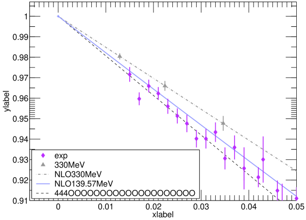
Figure 11: Pion electromagnetic form factor at low $Q^{2}$ (from [B⁺08e]).

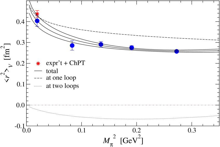
Figure 12: Pion charge radius in experiment and lattice QCD (from [J⁺08]).

An interesting study of the pion form factor for $n_{f}=2$ overlap fermions with Wilson kernel and the Iwasaki gauge action in a fixed topological sector has been presented recently by the JLQCD collaboration [J⁺08]. Results have been obtained for a lattice spacing of $a=0.118\text{ fm}$ in a volume of $V\approx(1.9\text{ fm})^{3}$, for four different pion masses ranging from very low $288$ to $522\text{ MeV}$. Using all-to-all propagators, a remarkable statistical precision was achieved with a comparatively small number of only $\mathcal{O}(100)$ configurations per ensemble. Contributions to the all-to-all propagators from the 100 lowest-lying modes of the overlap Dirac operator have been treated exactly, while the higher modes were stochastically estimated using $Z_{2}$ noise and the dilution method proposed in [F⁺05]. The $Q^{2}$-dependence of the pion vector form factor has been fitted with an ansatz based on the $\rho$-meson pole (monopole term) plus polynomial corrections, and the mean square pion charge radius and curvature term $c_{V}$ were extracted from the usual expansion $F_{\pi}(Q^{2})=1-6^{-1}\langle r_{\pi}^{2}\rangle Q^{2}+c_{V}(Q^{2})^{2}+\mathcal{O}(Q^{6})$. Figure 12 displays the resulting values for $\langle r_{\pi}^{2}\rangle$ as a function of $m_{\pi}^{2}$, which are somewhat low compared to the results discussed above by QCDSF/UKQCD and RBC-UKQCD in the overlapping region of $m_{\pi}\sim 300-500\text{ MeV}$. The result of a simultaneous chiral fit to $\langle r_{\pi}^{2}\rangle$ and $c_{V}$ based on $2$-loop (NNLO) chiral perturbation theory [GM91, BCT98] with four free parameters (LECs) is represented by the solid lines in Fig. 12. Interestingly, the 2-loop contribution, indicated by the dotted line, is found to be substantial, of $\mathcal{O}(20\%)$, in the region where lattice data points are available. Leading finite volume corrections have been included in the analysis of the pion vector form factor using 1-loop lattice regularized ChPT [BL05], from which it is expected that the pion charge radius decreases for $L\rightarrow\infty$. Finally, from a simultaneous 2-loop ChPT fit additionally including lattice results for the scalar charge radius, $\langle r_{\pi}^{2}\rangle_{S}$ (extracted from the scalar form factor using the ansatz $F^{S}_{\pi}(Q^{2})=F^{S}_{\pi}(0)(1-6^{-1}\langle r_{\pi}^{2}\rangle_{S}Q^{2}+c_{S}(Q^{2})^{2})$), a value of $\langle r_{\pi}^{2}\rangle=0.404\pm(22)_{\text{stat}}\pm(22)_{\text{sys}}\text{ fm}^{2}$ was found at the physical pion mass, where the systematic error is due to variations in some LECs and the fitting ranges.

To further substantiate this interesting analysis, it would be important to study possible effects from working in a fixed (trivial) topological sector in more detail.

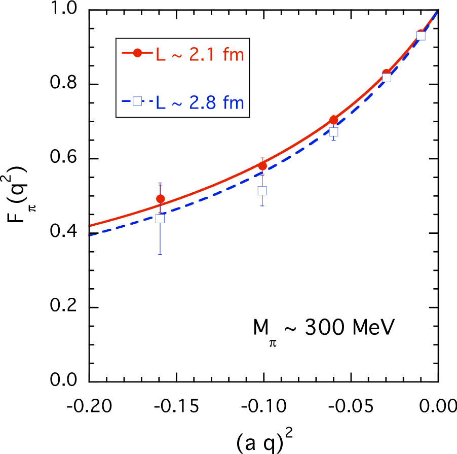
Figure 13: Pion form factor (from [Sim07]).

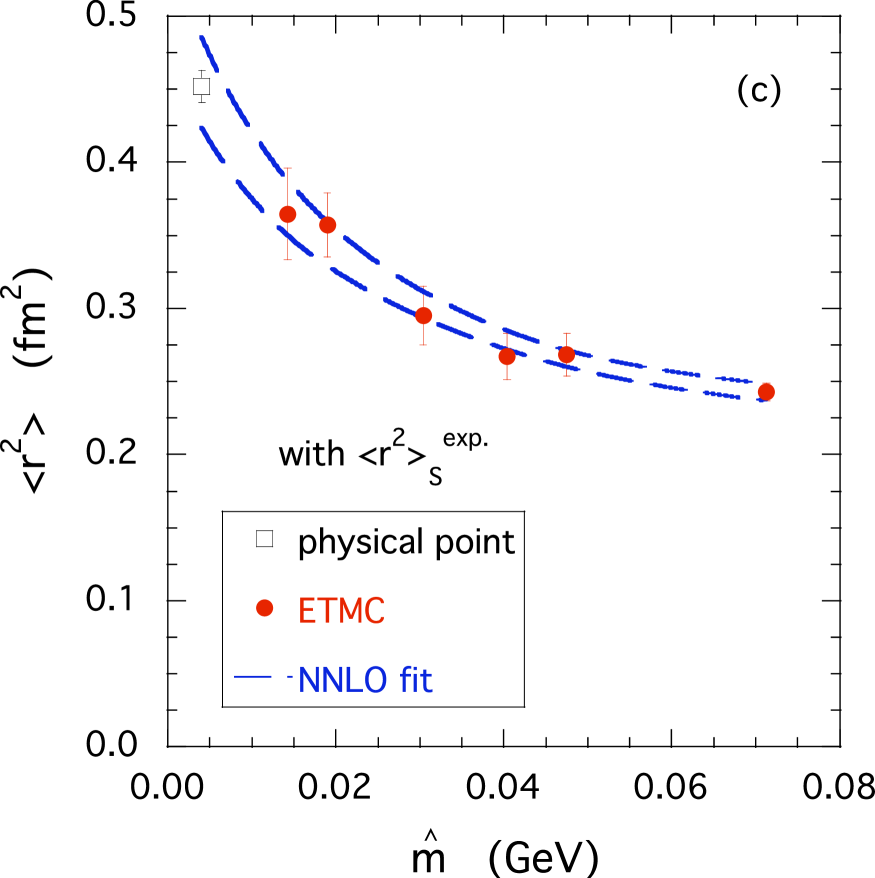
Figure 14: Pion mean square radius as function of the renormalized quark mass (from [FLS09]).

An extensive and detailed study of the pion form factor was presented recently by ETMC based on simulations with $n_{f}=2$ twisted mass fermions (tuned to maximal twist) and the tree-level improved Symanzik gauge action [FLS09]. Calculations were performed for six pion masses from $m_{\pi}\simeq 260\text{ MeV}$ to $m_{\pi}\simeq 580\text{ MeV}$, lattice spacings of $a\simeq 0.07\text{ fm}$ $a\simeq 0.09\text{ fm}$ and volumes of $V\approx(2.1\text{ fm})^{3}$, $V\approx(2.2\text{ fm})^{3}$ and $V\approx(2.8\text{ fm})^{3}$. All-to-all propagators based on the stochastic-source method and the “one-end-trick” described above and in sections 2.3.4, 2.3.5 were used together with partially twisted boundary conditions (pTBCs) (see section 2.3.6) to compute pion three-point functions in the Breit frame for (non-zero) $Q^{2}$ as low as $(Q^{2})^{\not=0}_{\text{min}}\approx 0.05\text{ GeV}^{2}$. Results for the pion form factor as a function of the squared momentum transfer in lattice units are displayed in Fig. 14 (note that $a^{-2}\approx 4.8\text{ GeV}^{2}$). A comparison of the lattice results for the two different volumes and with predictions from ChPT including pTBCs in a finite volume [JT08c] indicate that finite size effects are on the few-percent-level, of about the same size as the statistical errors. To minimize systematic uncertainties from FSE, the analysis was restricted to ensembles with $m_{\pi}L\gtrapprox 4$. Discretization effects were roughly estimated by comparing the main simulations results for $a\simeq 0.09\text{ fm}$ with a smaller number of results at $a\simeq 0.07\text{ fm}$ and found to be of the same order as the statistical uncertainties.

The $Q^{2}$-dependence of the lattice form factor data was fitted with a monopole ansatz, Eq. (129) with $m_{\text{mono}}(m_{\pi}^{2})=\text{const}$ as free parameter, as indicated in Fig. 14 by the solid line. From the fit, the mean square radius and curvature where obtained from $\langle r_{\pi}^{2}\rangle=6/m_{\text{mono}}^{2}$ and $c_{V}=1/m_{\text{mono}}^{4}$, respectively. Corresponding results for $\langle r_{\pi}^{2}\rangle$ are displayed in Fig. 14 as a function of the renormalized quark mass $\hat{m}\propto m_{\pi}^{2}+h.o.$ (see GMOR relation in Eq. (128)). The dashed lines represent the $1\sigma$ error band of a simultaneous chiral fit at NNLO to the lattice results for $\langle r_{\pi}^{2}\rangle$, $m_{\pi}^{2}(\hat{m})$, $f_{\pi}$ and $c_{V}$. In order to reduce the substantial uncertainties in the relevant low energy constants (fit parameters), in particular $\bar{l}_{i=1,\ldots,4}$, in the chiral fit, the experimental result for the scalar mean square radius of $\langle r_{\pi}^{2}\rangle^{\exp}_{S}=0.61\pm 0.04\text{ fm}^{2}$ was included and simultaneously fitted at NNLO together with the lattice results for the other observables mentioned before. The fit represented by the error band in Fig. 14 provides a very good description of the lattice data, and due to the singnificant upwards bending at low quark masses, the extrapolated result of $\langle r_{\pi}^{2}\rangle^{\text{phys}}=0.456\pm 0.030_{\text{stat}}\pm 0.024_{\text{sys}}$ fully overlaps with the experimental value at the physical point (indicated by the open square). Estimates of uncertainties from finite size and discretization effects have been added in quadrature to provide the systematic error. For the details of this extensive analysis, including the values of the numerous fitted low energy constants, we refer to the original publication [FLS09].

An overview and a direct comparison of the recent results for the pion charge radius discussed in this section will be given below in section 3.8, cf. Figs. 63 and 64.

First lattice results for the pion tensor form factor $B^{\pi}_{T10}(Q^{2})$ as defined in Eq. 9 will be discussed in section 4.4.7 in the context of moments of pion generalized parton distributions.

3.4 Nucleon form factors

3.4.1 Dirac and Pauli form factors

Figure 16 presents a typical comparison between results from a lattice QCD calculation [AKNT06] and experiment for the isovector Dirac, $F^{u-d}_{1}(Q^{2})$, and Pauli, $F^{u-d}_{2}(Q^{2})$, form factors. The lattice results are based on simulations with $n_{f}=2$ flavors of Wilson fermions at a lattice spacing of $a\approx 0.08$ fm (obtained from an extrapolation of the nucleon mass to the chiral limit) in volumes of $V\approx(1.9\text{ fm})^{3}$. The local vector current has been renormalized by demanding that $F^{u-d}_{1}(0)=1$. Overall, the lattice data shows small statistical errors and a smooth $Q^{2}$-dependence. The direct comparison in Fig. 16 exemplifies the substantial difference of the slope in $Q^{2}$ of lattice and experimental results. Concerning normalization and pion mass dependence of $F^{u-d}_{2}(Q^{2})$, we note that the lattice values were obtained using the continuum parametrization in Eq. 20 with $m_{N}=m_{N}^{\text{lat}}$, i.e. the pion mass, volume, and lattice spacing dependent nucleon mass for the corresponding ensemble. Empirically, it is known that the lattice nucleon mass drops approximately linearly in $m_{\pi}$ towards the physical point (see, e.g., [WL⁺08]), $m^{\text{lat}}_{N}\sim\text{const}+\alpha m_{\pi}$ with $\alpha\sim 1$, so that the choices $m_{N}=m_{N}^{\text{lat}}$ or $m_{N}=m_{N}^{\text{phys}}$ on the right-hand-side in Eq. 20 lead to noticeably different results for $F_{2}(Q^{2})$. This issue has been discussed in some detail in Ref. [G⁺05e] in connection with the chiral extrapolation of quenched lattice results from QCDSF/UKQCD, and should always be kept in mind when studying the pion mass dependence of the form factor $F^{u-d}_{2}(Q^{2})$ (for example in Fig. 16) and the anomalous magnetic moment $\kappa=F_{2}(0)$. Concerning $F^{u-d}_{1}(Q^{2})$, one finds that the overall $Q^{2}$-slope over the full range of $Q^{2}=0,\cdots,2.5\text{ GeV}^{2}$ changes only very little going from $m_{\pi}=0.69\text{ GeV}$ down to $m_{\pi}=0.38\text{ GeV}$.

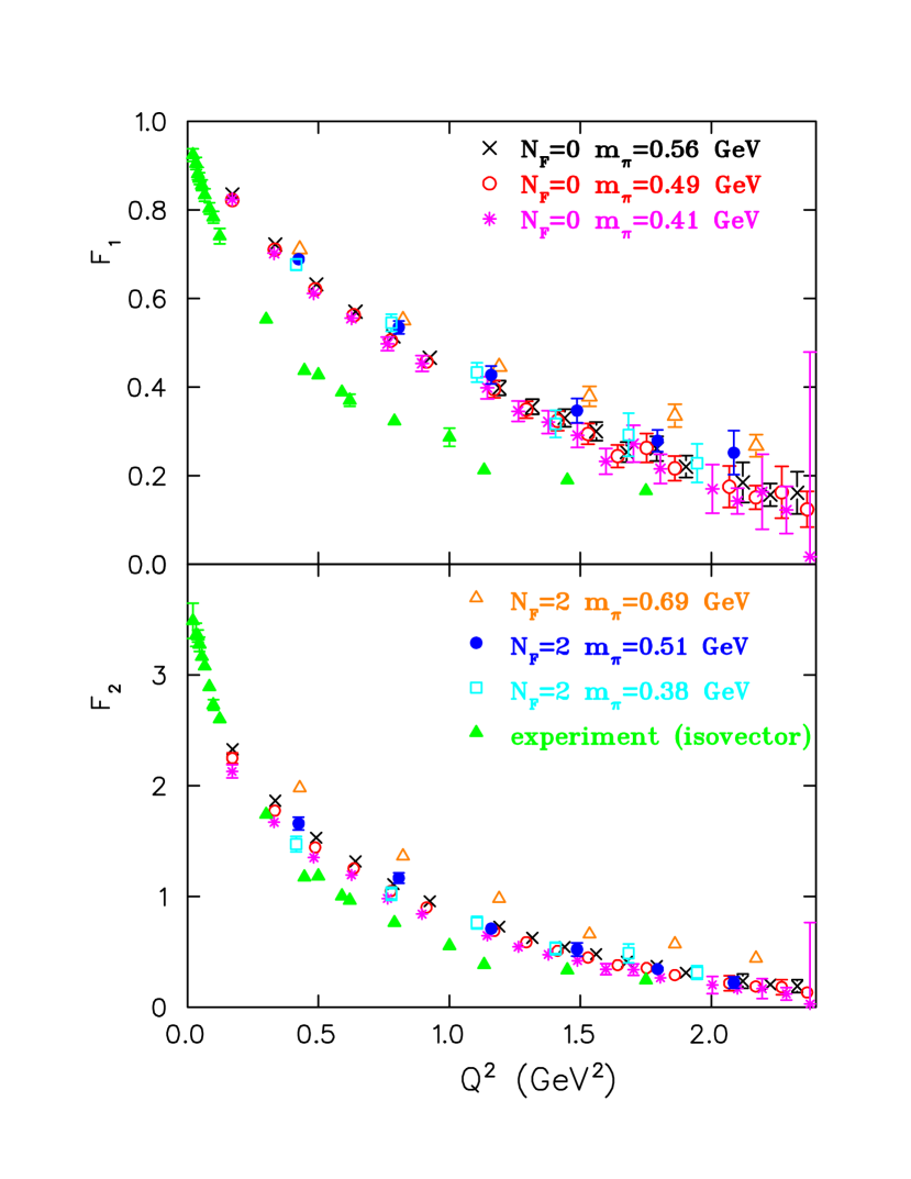
Figure 15: Nucleon form factors $F_{1}$ (top) and $F_{2}$ (bottom) in the isovector channel compared to experimental data (from [AKNT06]).

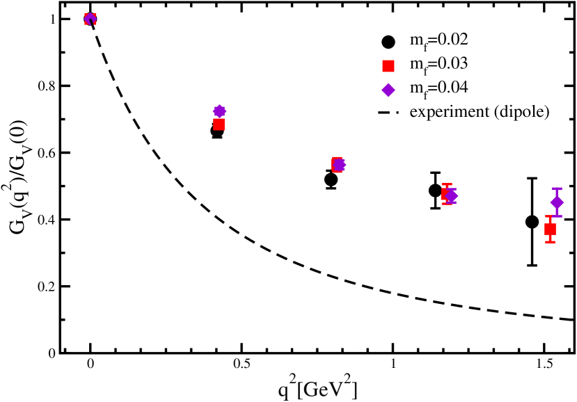
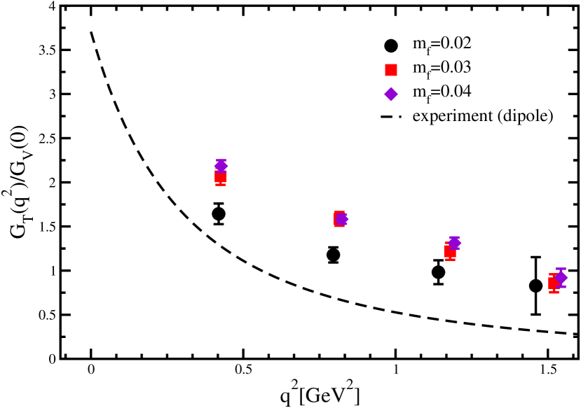
Figure 16: Nucleon form factors $F_{1}$ (top) and $F_{2}$ (bottom) in the isovector channel compared to dipole parametrizations of experimental data (from [LBO⁺08]).

Very similar observations can be made on the basis of recent results from the RBC collaboration for $n_{f}=2$ flavors of domain wall fermions and a doubly-blocked Wilson (DBW2) gauge action shown in Fig. 16 [LBO⁺08]. Results have been obtained for three different pion masses, $m_{\pi}=0.695,0.607,0.493\text{ GeV}$, at a lattice spacing of $a\approx 0.11$ fm, determined from a calculation and extrapolation of the mass of the $\rho$-meson, and for a volume of $V\approx(1.9\text{ fm})^{3}$. As above, the lattice nucleon mass has been used for the extraction of $F^{u-d}_{2}(Q^{2})$. The $Q^{2}$-slope of $F^{u-d}_{1}(Q^{2})$ from the lattice is again substantially flatter than for the phenomenological dipole fit describing the experimental data. At the same time, within statistical errors, there is no systematic pion mass dependence visible of the lattice data points for $F^{u-d}_{1}(Q^{2})$. Corresponding results for the Dirac mean square radius will be discussed in the following section, cf. Fig. 23. Preliminary results for the Dirac and Pauli form factors, based on configurations generated by RBC-UKQCD with $n_{f}=2+1$ flavors of domain wall fermions and the Iwasaki gauge action, have been presented recently by LHPC [S⁺08]. Gaussian-smeared sources with APE-smeared links and carefully tuned parameters were employed to obtain an optimal overlap with the nucleon ground state, supporting the use of a source-sink separation of $\approx 1.0\text{ fm}$ for the three-point functions. Coherent sequential propagators based on 4 nucleon and 4 anti-nucleon sources were employed to increase the statistics. Figures 18 and 18 show the $Q^{2}$-dependence of $F_{1}$ and $F_{2}$ in the isovector channel for pion masses from $\approx 298$ to $\approx 406\text{ MeV}$. Consistent results were obtained for the “fine” lattices, with an estimated lattice spacing of $\approx 0.084\text{ fm}$, and the “coarse” lattice with $a\approx 0.114\text{ fm}$. The spatial volumes are $V\approx(2.7\text{ fm})^{3}$ in both cases. As indicated by the dipole fits, the slope in $Q^{2}$ of both form factors slightly increases with decreasing pion masses, but even at the lowest pion mass the lattice data at non-zero $Q^{2}$ is still far above the experimental results.

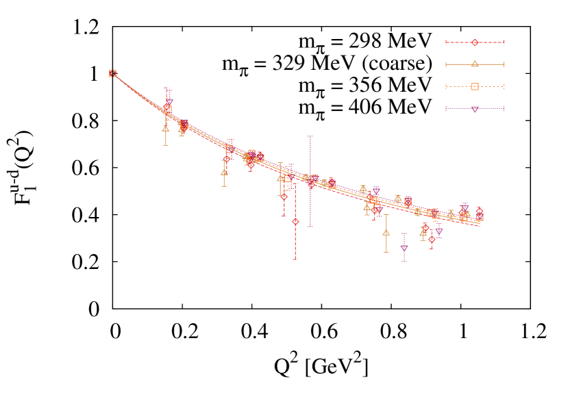
Figure 17: Isovector form factor $F_{1}$ together with dipole parametrization from (from proceedings [S⁺08]).

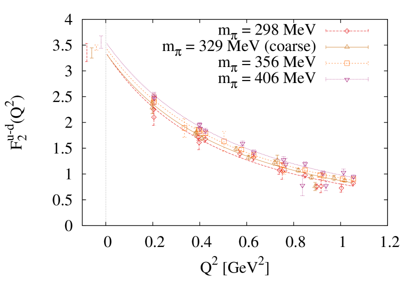
Figure 18: Isovector form factor $F_{2}$ together with dipole parametrization from (from proceedings [S⁺08]).

A preliminary comparison of a full $n_{f}=2+1$ DW calculation with a hybrid calculation for $n_{f}=2+1$ flavors of domain wall fermions and staggered Asqtad sea quarks, based on gauge configurations provided by the MILC collaboration, has been performed recently in [B⁺08f]. This careful studied revealed good consistency for $F_{1}^{u-d}$ of the full DW and the hybrid results with lattice spacings of $a\approx 0.084\text{ fm}$ and $a\approx 0.124\text{ fm}$, respectively, indicating that discretization effects are small. Volume effects in the case of the hybrid approach were also analyzed and found to be negligible within statistical errors.

3.4.2 Charge radii and anomalous magnetic moment

Over the last couple of years, the QCDSF-UKCQD collaboration has performed extensive hadron structure calculations using $n_{f}=2$ flavors of clover-improved Wilson fermions and Wilson gluons for a large number of pion masses, several lattice spacings and volumes. In [G⁺06c], the lattice data for the nucleon Dirac and Pauli form factors was fitted with a standard $p$-pole ansatz

$$F_{i}(Q^{2})=\frac{F_{i}(0)}{\left(1+\frac{Q^{2}}{p\,m_{i}^{2}}\right)^{p}}\,,$$ (132)

for $i=1,2$, choosing $p=2$ for $F_{1}$ and $p=3$ for $F_{2}$, and where $F_{2}(0)$ and $m_{i}$ were treated as free fitting parameters. The local vector current has been renormalized by demanding that $F^{u-d}_{1}(0)=1$. Results for the isovector mean square radius for $F_{1}$, Eq. (60), obtained from $\langle r_{1}^{2}\rangle=6/m_{1}^{2}$, are shown in Fig. 20 as a function of $m_{\pi}^{2}$. In [G⁺07a], a slightly more general ansatz has been used to describe the $Q^{2}$-dependence of $F_{1}$ and $F_{2}$,

$$F_{i}(Q^{2})=\frac{F_{i}(0)}{1+c_{i,2}Q^{2}+c_{i,2i+2}Q^{2i+2}}\,,$$ (133)

where $c_{i2}$, $c_{i4}$ and $F_{2}(0)$ are fitting parameters. Within the available statistics, both ansätze in Eq. (132) and Eq. (133) provided similarly good descriptions of the lattice data. Results for the Pauli form factor radius based on the parametrization in Eq. (133), with $\langle r_{2}^{2}\rangle=6c_{22}$, are displayed in Fig. 20 as a function of the pion mass. We note that the lattice data points in Fig. 20 and 20 correspond to a range of lattice spacings, $a\approx 0.67,\ldots,0.85\text{ fm}$ (chirally extrapolated) that have been fixed using the nucleon mass, and to different volumes from $V\approx(1.2\text{ fm})^{3}$ to $V\approx(1.9\text{ fm})^{3}$, with $m_{\pi}L>3.5$.

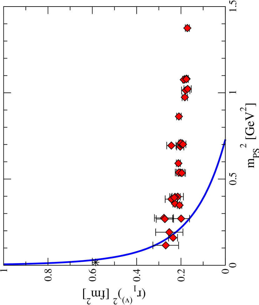
Figure 19: Isovector mean square charge radius for $F^{u-d}_{1}$ (from proceedings [G⁺06c]). Phenomenological value from [BHM07].

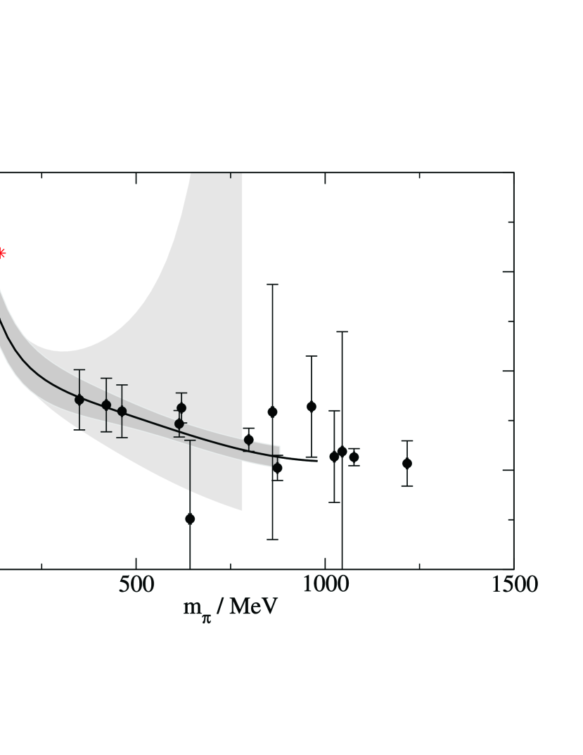
Figure 20: Isovector mean square radius for $F^{u-d}_{2}$ (from proceedings [G⁺07a]).

Within statistics, remarkably consistent results were obtained for $\langle r_{1}^{2}\rangle_{u-d}$ and $\langle r_{2}^{2}\rangle_{u-d}$ for the different ensembles (lattice spacings and volumes). Concerning the pion mass dependence, one finds that $\langle r_{1}^{2}\rangle_{u-d}$ is very slowly and approximately linearly rising over the full range from $m_{\pi}\sim 1.2\text{ GeV}$ down to $m_{\pi}\sim 0.330\text{ GeV}$, and that even at the lowest available pion mass the lattice result are roughly a factor of two below the experimental number $\langle r_{1}^{2}\rangle_{u-d}=0.635\pm 0.007\text{ fm}^{2}$ (PDG [A⁺08i]), in accordance with the discussion of Figs. 16 and 16 above. We note that a recent dispersion relation analysis of experimental data gives a smaller value $\langle r_{1}^{2}\rangle_{u-d}=0.585\pm 0.017$ [BHM07].

An explanation for the discrepancy between the lattice results and the experimental data may be given on the basis of chiral perturbation theory, which generically predicts that the isovector charge radius diverges logarithmically in the chiral limit. The chiral extrapolations indicated by the lines and bands in Figs. 20, 20 and 21 were based on the results developed in [HW02, G⁺05e] to $\mathcal{O}(\epsilon^{3})$ in the SSE of HBChPT. To this order, the pion mass dependence of $\langle r_{1}^{2}\rangle_{u-d}$ is given by [G⁺05e]

$$\langle r_{1}^{2}\rangle_{u-d}^{\text{SSE}} = -\frac{1}{(4\pi f_{\pi})^{2}}\left\{1+7g_{A}^{2}+\left(10g_{A}^{2}+2\right)\ln\left(\frac{m_{\pi}}{\lambda}\right)\right\}+\frac{c_{A}^{2}}{54\pi^{2}f_{\pi}^{2}}\Bigg{\{}26+30\ln\left(\frac{m_{\pi}}{\lambda}\right)$$ (134)

$$+ 30\frac{\Delta m_{\Delta N}}{\sqrt{\Delta m_{\Delta N}^{2}-m_{\pi}^{2}}}\ln\left(\frac{\Delta m_{\Delta N}}{m_{\pi}}+\sqrt{\frac{\Delta m_{\Delta N}^{2}}{m_{\pi}^{2}}-1}\right)\Bigg{\}}-\frac{12B_{10}^{(r)}(\lambda)}{(4\pi f_{\pi})^{2}}\,,$$

which, in addition to the counter term $B_{10}^{(r)}(\lambda)$ that removes the regularization scale dependence, is governed by four LECs: $f_{\pi}$, $g_{A}$, the axial transition pion-nucleon-$\Delta$ coupling constant $c_{A}=g_{\pi N\Delta}$, and $\Delta m_{\Delta N}$ (all in the chiral limit). Using their phenomenological values at the physical point as input, and setting the counter term equal to zero at a scale of $\lambda=600\text{ MeV}$ [G⁺05e], the SSE result provides a prediction for the $m_{\pi}$-dependence as indicated by the solid curve in Fig. 20. Clearly, at the given order, the SSE HBChPT formula is maximally applicable up to the lowest accessible lattice pion masses of $\approx 500\text{ MeV}$. At larger pion masses, the SSE prediction does not flatten off fast enough and therefore undershoots the lattice data points. However, it does provide a link between the lattice data at the lowest pion masses and the chiral limit. This indicates that future lattice results for $\langle r_{1}^{2}\rangle_{u-d}$ not much below $m_{\pi}\approx 300\text{ MeV}$ may show a strong upwards bending and therefore a clear deviation from the linear $m_{\pi}^{2}$ dependence. However, it should be noted that the SSE prediction also misses the experimental number by $\approx 20\%$, indicating that higher order corrections may be important already at the physical pion mass. A quantitative comparison with lattice results around or above $m_{\pi}^{\text{phys}}$ should therefore be considered with some caution.

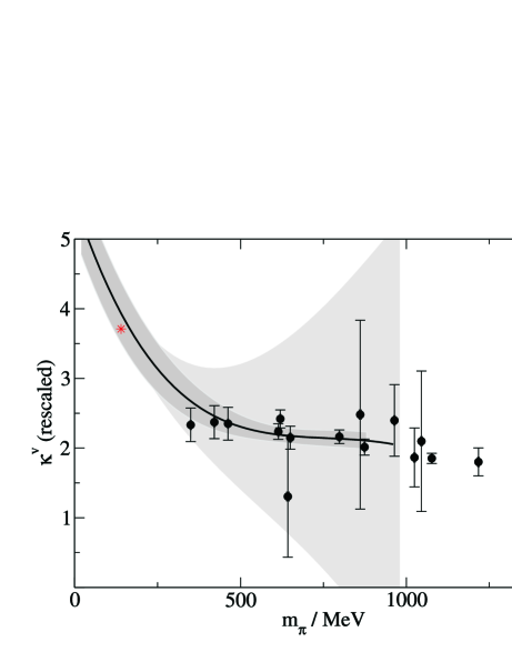
Figure 21: Isovector anomalous magnetic moment $\kappa^{u-d}$ (from proceedings [G⁺07a]).

We now come back to the results from QCDSF-UKQCD for the isovector mean square radius of $F_{2}$ shown in Fig. 20, obtained from the parametrization in Eq. (133). As for $\langle r_{1}^{2}\rangle_{u-d}$, the lattice results at the lowest available pion masses of $\approx 350$ to $\approx 400\text{ MeV}$ are $\approx 50\%$ below the experimental result, $\langle r_{2}^{2}\rangle_{u-d}=0.776\pm 0.011\text{ fm}^{2}$. In contrast to the isovector Dirac form factor, the Pauli form factor is predicted to diverge linearly as $1/m_{\pi}$ in the chiral limit. To $\mathcal{O}(\epsilon^{3})$ in SSE HBChPT, the pion mass dependence of $\langle r_{2}^{2}\rangle_{u-d}$ is given by [G⁺05e]

$$\langle r_{2}^{2}\rangle_{u-d}^{\text{SSE}}=\frac{m_{N}}{\kappa_{u-d}(m_{\pi})}\Bigg{\{}\frac{g_{A}^{2}}{8\pi f_{\pi}^{2}m_{\pi}}+\frac{c_{A}^{2}}{9\pi^{2}f_{\pi}^{2}\sqrt{\Delta m_{\Delta N}^{2}-m_{\pi}^{2}}}\ln\left(\frac{\Delta m_{\Delta N}}{m_{\pi}}+\sqrt{\frac{\Delta m_{\Delta N}^{2}}{m_{\pi}^{2}}-1}\right)+24B_{c2}\Bigg{\}}\,$$ (135)

and involves, in addition to the LECs discussed above, also the (pion mass dependent) isovector anomalous magnetic moment $\kappa_{u-d}(m_{\pi})$ and the constant $B_{c2}$. The SSE expression for $\kappa_{u-d}$ reads [G⁺05e]

$$\kappa_{u-d}^{\text{SSE}} = \kappa_{u-d}^{0}-\frac{g_{A}^{2}\,m_{\pi}m_{N}}{4\pi F_{\pi}^{2}}+\frac{2c_{A}^{2}\Delta m_{\Delta N}m_{N}}{9\pi^{2}F_{\pi}^{2}}\Bigg{\{}\sqrt{1-\frac{m_{\pi}^{2}}{\Delta m_{\Delta N}^{2}}}\ln\left(\frac{\Delta m_{\Delta N}}{m_{\pi}}+\sqrt{\frac{\Delta m_{\Delta N}^{2}}{m_{\pi}^{2}}-1}\right)$$ (136)

$$+ \ln\left(\frac{m_{\pi}}{2\Delta m_{\Delta N}}\right)\Bigg{\}}+\frac{4c_{A}c_{V}g_{A}m_{N}m_{\pi}^{2}}{9\pi^{2}F_{\pi}^{2}}\ln\left(\frac{2\Delta m_{\Delta N}}{\lambda}\right)+\frac{4c_{A}c_{V}g_{A}m_{N}m_{\pi}^{3}}{27\pi F_{\pi}^{2}\Delta m_{\Delta N}}$$

$$- \frac{8c_{A}c_{V}g_{A}\Delta m_{\Delta N}^{2}m_{N}}{27\pi^{2}F_{\pi}^{2}}\Bigg{\{}\left(1-\frac{m_{\pi}^{2}}{\Delta m_{\Delta N}^{2}}\right)^{3/2}\ln\left(\frac{\Delta m_{\Delta N}}{m_{\pi}}+\sqrt{\frac{\Delta m_{\Delta N}^{2}}{m_{\pi}^{2}}-1}\right)$$

$$+ \left(1-\frac{3m_{\pi}^{2}}{2\Delta m_{\Delta N}^{2}}\right)\ln\left(\frac{m_{\pi}}{2\Delta m_{\Delta N}}\right)\Bigg{\}}-8E_{1}^{(r)}(\lambda)m_{N}m_{\pi}^{2}\,,$$

and depends on two more LECs, the isovector anomalous magnetic moment $\kappa^{0}_{u-d}$ and the isovector nucleon-$\Delta$ transition coupling constant $c_{V}=c^{0}_{V}$ in the chiral limit, as well as an additional scale dependent counter term parameter $E_{1}^{(r)}(\lambda)$. They were treated as free parameters in a simultaneous fit of the SSE HBChPT formulas for the mean square radius $\langle r_{2}^{2}\rangle_{u-d}$ (Eq. 135) and $\kappa_{u-d}$ to the lattice data points in Figs. 20 and 21, obtained from the more general ansatz Eq. (133). The fit result for $\langle r_{2}^{2}\rangle_{u-d}$ is shown in Fig. 20 as smaller error band, where the width of the band represents the statistical errors only. Although the SSE chiral extrapolation provides some curvature towards the physical point, it still underestimates the experimental result by $\approx 25\%$. We note that results for $\langle r_{2}^{2}\rangle_{u-d}$ and $\kappa^{u-d}$ based on the $p$-pole ansatz in Eq. (132) (presented in [G⁺06c] but not shown here) lead to visibly different chiral fits, with a central extrapolation curve for $\langle r_{2}^{2}\rangle_{u-d}$ that is up to $25\%$ below the one in Fig. 20. This reveals that the ansatz used to parametrize the form factors can have a significant impact on the resulting chiral extrapolation. Similar results also hold for the anomalous magnetic moment, as we will discuss in the following.

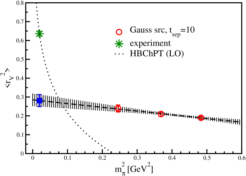
Figure 22: Isovector Dirac rms radius from RBC for $n_{f}=2$ flavors of DW fermions (from [LBO⁺08]). Experimental value from the PDG [A⁺08i].

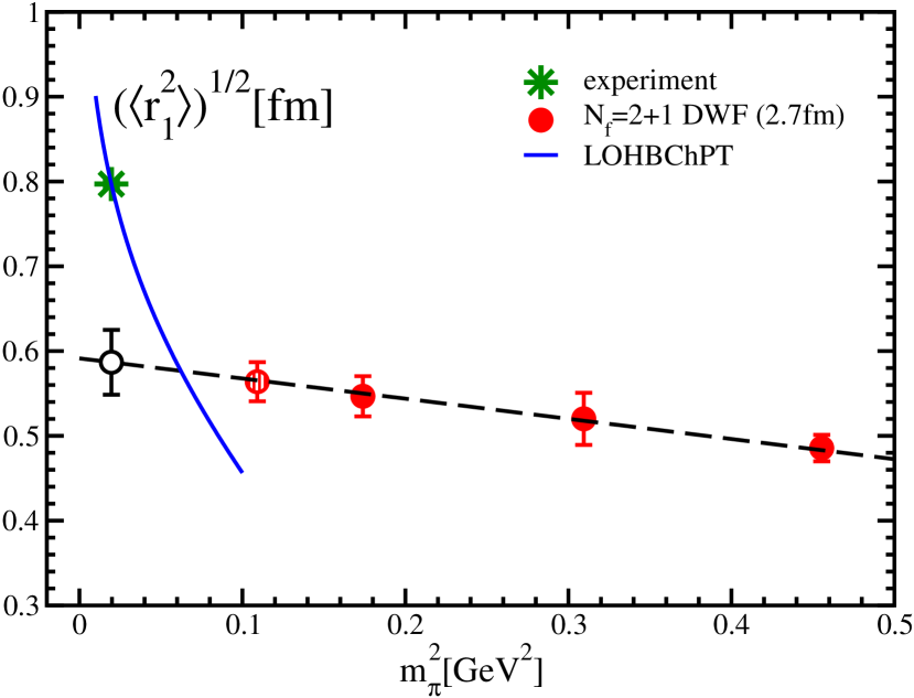
Figure 23: Isovector Dirac rms radius from RBC-UKQCD $n_{f}=2+1$ flavors of DW fermions with $t_{\text{sep}}=12$ (from lattice proceedings [OY08]). Experimental value from the PDG [A⁺08i].

The lattice data points in Fig. 21 were obtained from the parametrization in Eq. (133), providing the required extrapolations of the Pauli form factor lattice data at non-zero momentum transfer to $Q^{2}=0$. The results for $\kappa_{u-d}$ were scaled with a factor of $m_{N}^{phys}/m_{N}^{lat}(m_{\pi})$ to remove the additional pion mass dependence that comes in through the use of the pion mass dependent nucleon mass in the extraction of $F_{2}$, as explained above. Although slowly rising towards lower pion masses, the lattice results still lie $\approx 25\%$ below the experimental value at the lowest pion masses of $\approx 350$ to $\approx 400\text{ MeV}$. The chiral extrapolation of the lattice results based on a simultaneous fit to $\langle r_{2}^{2}\rangle_{u-d}$ and $\kappa_{u-d}$ (based on Eq. (135) and Eq. (136)) as discussed above is presented by the error band in Fig. 21. It is promising to see that the chiral fit overlaps within errors with the value from experiment. Such an agreement within errors between extrapolated lattice results and experiment could not be observed on the basis of the $p$-pole ansatz in Eq. 132 used in [G⁺06c]. We note, however, that the lattice values for $\langle r_{2}^{2}\rangle_{u-d}$ and $\kappa_{u-d}$ obtained from the more general ansatz in Eq. (133) have larger errors than the results from the $p$-pole parametrization, and a comparison of the two approaches is at this point clearly limited by statistics. Still, we conclude that different methods to parametrize and extrapolate nucleon form factors to $Q^{2}=0$ may lead to significantly different final results, in particular for $F_{2}(Q^{2})$ and in combination with a chiral extrapolation to the physical point. This is a serious source of systematic uncertainty, and below in sections 3.6, 3.7, 6.0.4, we will discuss some alternative and also new approaches, for example based on background field methods and pTBCs to access small non-zero $Q^{2}$, which may help to improve the situation in the near future. For a detailed discussion of chiral fits based on Eqs. (134), (135) and (136) to quenched lattice data and of the corresponding LECs, we refer to [G⁺05e].

Results for the isovector Dirac rms radius from the RBC collaboration, based on $n_{f}=2$ flavors of domain wall fermions for a lattice spacing of $a\approx 0.11$ fm and a volume of $V\approx(1.9\text{ fm})^{3}$, are shown in Fig. 23 [LBO⁺08]. The rms radius has been obtained from dipole fits to the form factor data displayed in Fig. 16. The results, which are in overall agreement with the lattice data from QCDSF-UKQCD presented in Fig. 20, are more than a factor of two below the experimental value and only show a hint of a slope in $m_{\pi}^{2}$, so that a linear extrapolation in $m_{\pi}^{2}$ to the physical pion mass fails dramatically. As mentioned already above, LO HBChPT predicts a strong non-linear pion mass dependence at lower pion masses (represented by the dashed line), clearly indicating that an extrapolation linear in $m_{\pi}^{2}$ is most probably misleading in this case.

More recently, RBC-UKQCD presented results for the Dirac and Pauli form factor based on simulations with $n_{f}=2+1$ flavors of domain wall fermions and the Iwasaki gauge action [OY08] (for simulation details, see [A⁺08h]). Calculations were performed for pion masses of $\simeq 331$, $\simeq 419$, $\simeq 557$ and $\simeq 672\text{ MeV}$, a lattice spacing of $a\simeq 0.114\text{ fm}$ and volumes of $\simeq(1.82\text{ fm})^{3}$ and $\simeq(2.74\text{ fm})^{3}$. Bare quark masses and the lattice scale were fixed using $SU(2)$ ChPT fits and experimental values for the $\pi$, $K$ and $\Omega$ meson masses. The dynamical lattice strange quark mass turned out to be $\approx 12-15\%$ larger than the physical strange quark mass. A comparatively large sink-source time separation of $t_{\text{sep}}=12$ units corresponding to $\approx 1.37\text{ fm}$ was chosen for the nucleon three-point functions in order minimize contaminations from excited states, which in principle could be very helpful in reducing this sort of systematic error. In practice, however, while statistically clean plateaus for the ratio of three- to two-point functions could be observed for $t_{\text{sep}}=10$ , the statistics is notably worse for $t_{\text{sep}}=12$, to an extent that it may even be difficult to identify a proper plateau region in the first place, see for example Fig. 76 by RBC related to moments of PDFs. Furthermore, we note that the nucleon two point functions that enter the ratio of three- to two-point functions in Eq. (110) in particular at the sink position $t_{\text{snk}}$, may show significant fluctuations at large times. Therefore, while excited states may contaminate the plateau for too small $t_{\text{snk}}$, choosing a specific large source-sink separation may introduce an additional systematic uncertainty through $C_{\text{2pt}}(t_{\text{snk}})$.

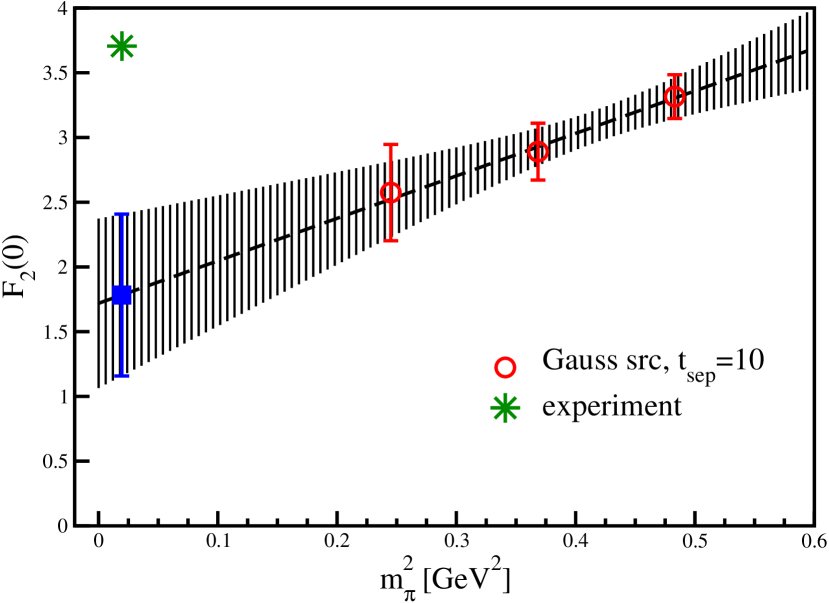
Figure 24: Isovector anomalous magnetic moment for $n_{f}=2$ flavors of DW fermions (from [LBO⁺08]).

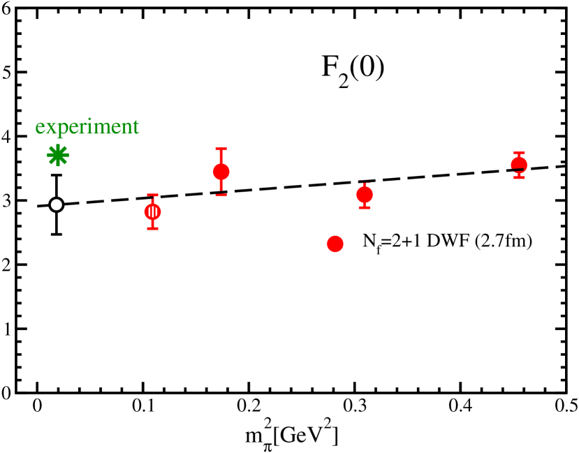
Figure 25: Isovector anomalous magnetic moment for $n_{f}=2+1$ flavors of DW fermions with $t_{\text{sep}}=12$ (from proceedings [OY08]).

Figure 23 shows the pion mass dependence of the Dirac rms radius from these $n_{f}=2+1$ simulations, as obtained from dipole fits to $F_{1}(Q^{2})$. Even at the lowest accessible pion mass of $\simeq 331\text{ MeV}$, no sign of an upwards bending is visible. Consequently, the notorious linear extrapolation to the physical pion mass, represented by the dashed line, fails. A comparison of Fig. 23 and Fig. 23, shows that the $n_{f}=2+1$ results lie systematically above than the values obtained for $n_{f}=2$ flavors of DW fermions. Though the effect is not dramatic within statistical errors, it would be interesting to find out if this is related to a systematic uncertainty, e.g. the setting of the scale or the different source-sink separations, or a genuine effect due to the dynamical strange quark.

Results for the isovector anomalous magnetic moment, $\kappa_{u-d}$, from RBC and RBC-UKQCD for $n_{f}=2$ and $n_{f}=2+1$ flavors of DW fermions are displayed in Fig. 25 and Fig. 25, respectively. Note that in both cases the pion mass dependent lattice nucleon mass has been used to extract $F^{u-d}_{2}(Q^{2})$ (cf. Eq.20), which was then fitted with a dipole ansatz and extrapolated to $Q^{2}=0$ to obtain $\kappa_{u-d}=F^{u-d}_{2}(0)$. While the linear chiral extrapolation of the $n_{f}=2+1$ lattice data to the physical pion mass gives a value that is almost compatible within errors with the number from experiment, it clearly fails in the case of the $n_{f}=2$ results. The latter shows that a naive linear extrapolation of a small number of data points lacking sufficient statistical precision may be very misleading.

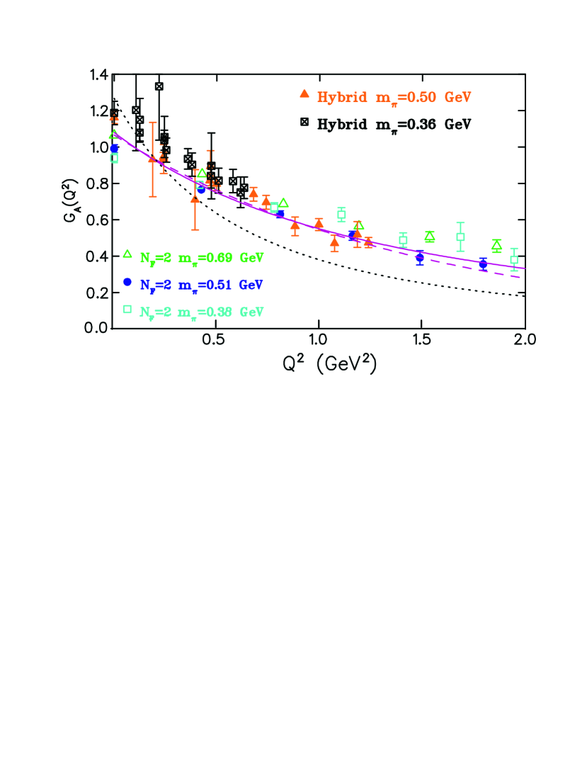
Figure 26: Isovector axial vector form factor $G^{u-u}_{A}(Q^{2})$ (from [AKL⁺07]; the figure has been edited for this review).

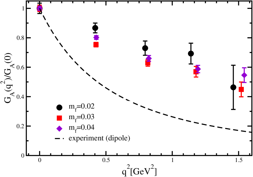
Figure 27: Normalized isovector axial vector form factor $G^{u-d}_{A}(Q^{2})/G^{u-d}_{A}(0)$ for $n_{f}=2$ flavors of DW fermions (from [LBO⁺08]).

3.4.3 Axial vector and pseudoscalar form factor

All results discussed in this section have been non-perturbatively renormalized. For the details, we refer to the original works.

Having discussed the vector form factors, we now turn our attention towards the axial-vector form factors of the nucleon. Figure 27 shows results for the proton isovector axial-vector form factor $G^{u-d}_{A}(Q^{2})$ from the Athens-Cyprus-MIT collaboration [AKL⁺07] for $n_{f}=2$ flavors of Wilson fermions together with corresponding results based on the $n_{f}=2+1$ hybrid calculation from LHPC, for pion masses as indicated in the legends. The underlying axial-vector currents have been non-perturbatively renormalized based on Refs. [B⁺06a, E⁺06a]. We first note that the normalizations of the lattice data, i.e. the forward limit values $g_{A}=G_{A}(Q^{2}=0)$, do not agree for the different dataset. In particular, the result from the hybrid calculation does not agree with the Wilson fermion result at similar pion masses, i.e. for $m_{\pi}\sim 500,510\text{ MeV}$ and $m_{\pi}\sim 360,380\text{ MeV}$. Possible reasons for such discrepancies, as well as the pion mass dependence of $g_{A}$ will be discussed in a separate paragraph below. Apart from the normalization, and considering the scatter at the lower pion masses, there is overall good agreement of the lattice data points within statistical errors . Specifically, there is no clear systematic pion mass dependence visible at larger $Q^{2}$, and the slope in $Q^{2}$ seems to be approximately independent of $m_{\pi}$. This observation is in agreement with the $n_{f}=2$ domain wall fermion data from RBC [LBO⁺08] for $G^{u-d}_{A}(Q^{2})/G^{u-d}_{A}(0)$ displayed in Fig. 27, where for example at $Q^{2}\sim 0.4\text{ GeV}$ the lattice value is first decreasing going from $m_{\pi}=695\text{ MeV}$ to $m_{\pi}=607\text{ MeV}$, only to increase to an even larger value for $m_{\pi}=493\text{ MeV}$. It has been speculated that this increase at the lowest pion mass is a finite volume effect [LBO⁺08], which would be quite remarkable considering that $m_{\pi}L\approx 4.75$ for this ensemble. In any case, the $Q^{2}$-slope of the lattice results shown in Figs. 27 and 27 is consistently much flatter than the one observed in experiment, represented by the dashed dipole curves.

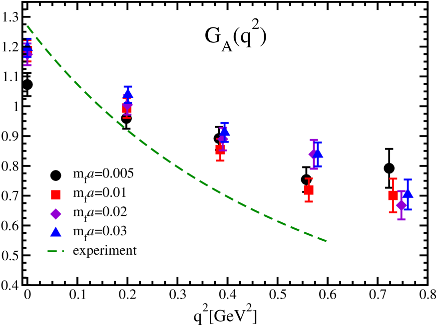
Figure 28: Isovector axial vector form factor $G^{u-u}_{A}(Q^{2})$ for $n_{f}=2+1$ flavors of DW fermions with (from proceedings [OY08]).

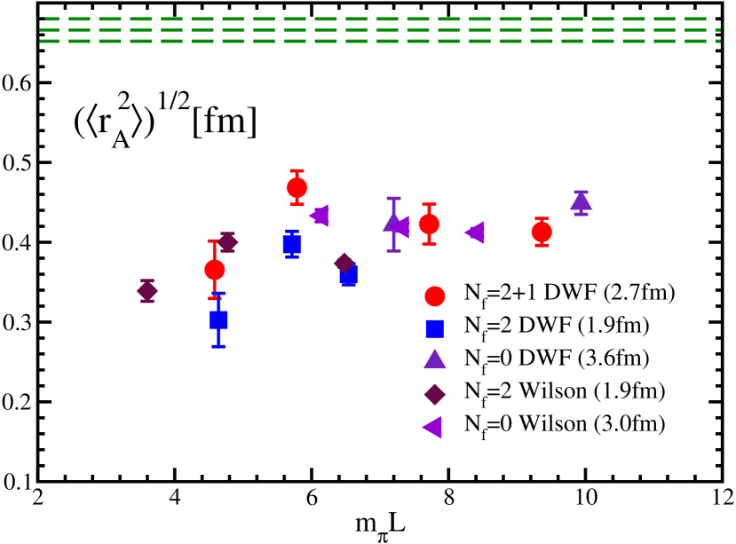
Figure 29: Isovector axial vector rms radius (from proceedings [OY08]).

More recent results from RBC-UKQCD for $G^{u-d}_{A}(Q^{2})$, for $n_{f}=2+1$ flavors of DW fermions are shown in Fig. 29 [OY08]. The different quark masses $m_{u}=m_{d}$ in the legend correspond to pion masses of $\approx 331$, $\approx 419$, $\approx 557$ and $\approx 672\text{ MeV}$. Apart from the results for the lightest quark mass, $ma=0.005$, which may be subject to finite volume effects, the lattice data points seem to come closer to the experimental result (indicated by the dashed line) as the quark mass decreases.

An overview of different dynamical and quenched lattice calculations, including the $n_{f}=2+1$ DW fermion results, of the axial vector radius $\langle r_{A}^{2}\rangle^{1/2}$ obtained from dipole fits to $G^{u-d}_{A}(Q^{2})$, is given in Fig. 29 [OY08]. The data points lie in a range of $\langle r_{A}^{2}\rangle^{1/2}=\approx 0.3,\ldots,0.5\text{ fm}$ and are significantly below experiment indicated by the dashed lines, where values between $\langle r_{A}^{2}\rangle^{1/2}=0.57\text{ fm}$ and $0.72\text{ fm}$ have been reported (see, e.g., the discussion in [SFGS07]). We note that lattice results for $m_{\pi}L\lessapprox 5$ are somewhat lower than the rest, however contrary to the claim in [OY08], no clear “scaling” in $m_{\pi}L$ can be observed. In particular the data points with $m_{\pi}L\approx 6.0,\ldots,6.5$ scatter significantly, indicating that other systematic effects related to the pion mass dependence, the range of $Q^{2}$ used in the underlying dipole fits, the setting of the scale, etc., are relevant in this case.

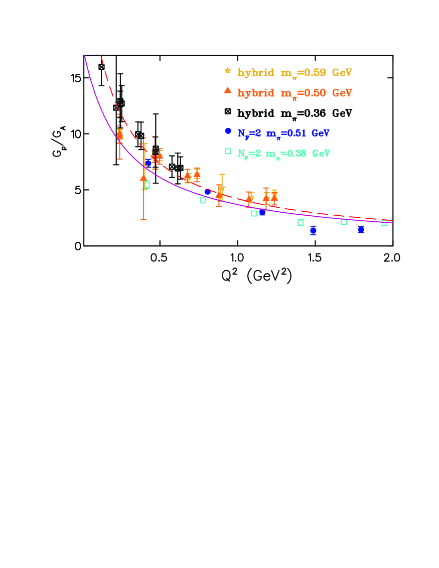
Figure 30: Ratio $\big{(}G^{u-d}_{A}/G^{u-d}_{P}\big{)}(Q^{2})$ (from [AKL⁺07]; the figure has been edited for this review).

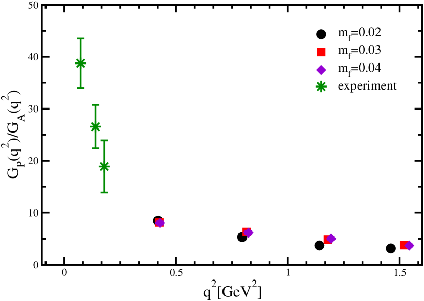
Figure 31: Ratio $\big{(}G^{u-d}_{A}/G^{u-d}_{P}\big{)}(Q^{2})$ (from [LBO⁺08]).

Results for the induced pseudo-scalar form factor in form of the ratio $\big{(}G^{u-d}_{P}/G^{u-d}_{A}\big{)}(Q^{2})$ from the Athens-Cyprus-MIT collaboration are shown in Fig. 31, for the same ensembles and lattice data as in Fig. 27. The ratio decreases rapidly for larger $Q^{2}$ as is expected from pion pole dominance, which states that

$$\frac{G^{u-d}_{P}(Q^{2})}{G^{u-d}_{A}(Q^{2})}\sim\frac{4m_{N}^{2}}{m_{\pi}^{2}+Q^{2}}\,.$$ (137)

This is plotted for comparison as dashed line in Fig. 31 for a lattice pion and nucleon mass of $m_{\pi}=0.411\text{ GeV}$ and $m_{N}=1.109\text{ GeV}$ respectively, and describes the overall trend of the lattice data well. While the results of the hybrid calculation appear to be overall consistent within errors, some discrepancies are visible for the $n_{f}=2$ Wilson fermion results. Specifically, taking into account that the ratio in Fig. 31 is independent of renormalization issues, it is quite remarkable that the values obtained from the $n_{f}=2$ Wilson fermion calculation are $\approx 40\%$ below the result from the $n_{f}=2+1$ hybrid calculation, at the lowest pion masses of $m_{\pi}\approx 360,\ldots,370\text{ MeV}$ and for a momentum transfer squared of $Q^{2}\approx 0.4\text{ GeV}$. Since for the Wilson fermion data point $m_{\pi}L\sim 3.5$, in comparison to a much larger value of $m_{\pi}L\sim 6.25$ for the hybrid case, it may be that finite volume effects are at least partially responsible for the observed discrepancy.

Figure 31 displays results for $\big{(}G^{u-d}_{P}/G^{u-d}_{A}\big{)}(Q^{2})$ from the $n_{f}=2$ domain wall fermion calculation by RBC [LBO⁺08], together with experimental data points from [C⁺93]. Although the experimental errors are rather large, Fig. 31 still shows exemplary the steep rise at lower values of the momentum transfer squared that may be observed in future lattice studies of $G_{P}(Q^{2})$ at lower pion masses and smaller $Q^{2}$.

3.4.4 Axial vector coupling constant

Having discussed the $Q^{2}$-dependence of the axial-vector and induced pseudo-scalar form factors, we now turn our attention to the axial-vector coupling, $g_{A}$, which we identify with the forward value of the nucleon axial-vector form factor, $g_{A}=G_{A}(Q^{2}=0)$, see Eq. (59). In the following, we will be concentrating on the isovector channel, $g_{A}=g^{u-d}_{A}$. Results for $g^{u+d}_{A}=\Delta\Sigma^{u+d}=G^{u+d}_{A}(Q^{2}=0)$ in the isosinglet channel will be presented in the framework of the nucleon spin structure in section 4.4.3 below.

Noting that the isovector axial vector coupling constant, $g^{u-d}_{A}$, plays a central role in QCD low energy dynamics, that it can be comparatively easily accessed on the lattice through the local isovector axial vector current, and that its experimental value is rather well known, it may be seen as an important “benchmark observable” for lattice QCD calculations [E⁺05]. Experimentally, it is known to high statistical precision from neutron beta decay, with an average value of $g_{A}=1.2695(29)$ from the PDG [A⁺08i]. The QCDSF-UKQCD collaboration has studied $g_{A}$ on the basis of a large number of ensembles for different pion masses in the range of $m_{\pi}\approx 600\text{ MeV}$ to $m_{\pi}\approx 1200\text{ MeV}$, lattice spacings from $a\approx 0.07\text{ fm}$ to $a\approx 0.11\text{ fm}$ and different volumes from $V\approx(0.95\text{ fm})^{3}$ to $V\approx(2.0\text{ fm})^{3}$, using $n_{f}=2$ flavors of improved Wilson fermions [K⁺06]. An overview of the results plotted versus $m_{\pi}^{2}$ is given in Fig. 33. To understand the distribution of the lattice data points in Fig. 33, it is important to note that the two lowest lying points correspond to finite volume simulations with smallest lattice volumes of only $V\approx(1.0\text{ fm})^{3}$. At least one more low lying point for $\beta=5.29$ can be identified that also correspond to a finite volume calculation with $V\approx(1.3\text{ fm})^{3}$, while the bulk of the lattice data points in Fig. 33 was obtained for larger volumes. This strongly indicates that finite volume effects may be significant, i.e. larger than $10\%$, for $m_{\pi}L<4$.

Noting that the inclusion of the $\Delta(1232)$-resonance is crucial to obtain value of $g_{A}$ larger than $1$ from the Adler-Weisberger sum rule, the pion mass dependence of $g_{A}$ has been worked out to $\mathcal{O}(\epsilon^{3})$ SSE-HBChPT (with explicit $\Delta$-intermediate states) in [HPW03] in infinite volume. This has been extended to finite volume in [Wol05, K⁺06] in the framework of the SSE of HBChPT, and a similar finite volume calculation of $g_{A}$ with explicit $\Delta$-DOFs can also be found in [BS04]. The result can be written as $g_{A}(L)=g_{A}(L=\infty)+\Delta g_{A}(L)$, with

$$g^{\text{SSE}}_{A}(L=\infty) = g_{A}^{0}+\left\{4\,B_{9}^{r}(\lambda)-8\,g_{A}^{0}B_{20}^{r}(\lambda)-\frac{(g_{A}^{0})^{3}}{16\pi^{2}f_{\pi}^{2}}-\frac{25c_{A}^{2}g_{1}}{324\pi^{2}f_{\pi}^{2}}+\frac{19c_{A}^{2}g_{A}^{0}}{108\pi^{2}f_{\pi}^{2}}\right\}m_{\pi}^{2}$$ (138)

$$- \left((g^{0}_{A})^{3}+\frac{1}{2}\,g^{0}_{A}\right)\frac{m_{\pi}^{2}}{4\pi^{2}f_{\pi}^{2}}\ln{\left(\frac{m_{\pi}}{\lambda}\right)}+\frac{4c_{A}^{2}g_{A}^{0}}{27\pi\Delta f_{\pi}^{2}}\,m_{\pi}^{3}$$

$$+ \left(25c_{A}^{2}g_{1}\Delta^{2}-57c_{A}^{2}g_{A}^{0}\Delta^{2}-24c_{A}^{2}g_{A}^{0}m_{\pi}^{2}\right)\frac{\sqrt{m_{\pi}^{2}-\Delta^{2}}}{81\pi^{2}f_{\pi}^{2}\Delta}\arccos\left(\frac{\Delta}{m_{\pi}}\right)$$

$$+ \frac{25c_{A}^{2}g_{1}\left(2\Delta^{2}-m_{\pi}^{2}\right)}{162\pi^{2}f_{\pi}^{2}}\ln\left(\frac{2\Delta}{m_{\pi}}\right)+\frac{c_{A}^{2}g_{A}^{0}\left(3m_{\pi}^{2}-38\Delta^{2}\right)}{54\pi^{2}f_{\pi}^{2}}\ln\left(\frac{2\Delta}{m_{\pi}}\right)$$

to $\mathcal{O}(\epsilon^{3})$ in the SSE [HPW03, K⁺06]. The expansion involves the LECs $f_{\pi}$, $g^{0}_{A}$, $c_{A}=g_{\pi N\Delta}$, $\Delta m_{N\Delta}$, $g_{1}$ (all in the chiral limit) and the scale dependent counter-terms $B^{r}_{9,20}(\lambda)$. For the complete (somewhat lengthy) expression for $\Delta g_{A}(L)$ at $\mathcal{O}(\epsilon^{3})$, we refer to [Wol05, K⁺06]. Since the finite volume formulas are essentially obtained from infinite volume expressions by replacing momentum integrals by sums over discrete momentum modes, $\mathbf{p}=2\pi/L\mathbf{n}$ with integer $\mathbf{n}_{i}$, $\Delta g_{A}(L)$ does not depend on any additional LECs. On the technical side, we note that the counter terms in [K⁺06] have been redefined compared to [HPW03] in order to match the definitions in HBChPT (without explicit $\Delta$-DOFs), which allows for a direct comparison of the LECs in HBChPT and SSE HBChPT to the given order. Treating the counter term and the couplings $g_{A}$ and $g_{1}$ as free parameters, while fixing the other LECs to their physical or chiral limit values known from the literature, the finite volume SSE HBChPT result has been fitted to all lattice data points with $m_{\pi}<770\text{ MeV}$ (including all volumes) in Fig. 33. The resulting prediction of the volume dependence of $g_{A}$ is displayed as solid line and compared to lattice data points in Fig. 33 for a pion mass of $\approx 770\text{ MeV}$. Keeping in mind that simulation results for rather large values of $m_{\pi}$ have been taken into account in the fit, the SSE HBChPT result describes the lattice data surprisingly well within the statistical errors. In a second step, the fit results were used to shift the lattice data points to the infinite volume limit by subtracting the finite volume correction, $\Delta g_{A}(L)=g_{A}(L)-g_{A}(L=\infty)$, from the lattice data points, $g_{A}^{\text{lat}}(L=\infty)=g_{A}^{\text{lat}}(L)-\Delta g_{A}(L)$, at the given pion masses. The resulting data points together with the infinite volume chiral extrapolation are shown Fig. 36, where in contrast to Fig. 33 only lattice data for $m_{\pi}<630\text{ MeV}$, represented by the filled symbols, have been taken into account in the chiral fit. Compared to Fig. 33 one finds that the different finite volume lattice data points for $g_{A}$ have been shifted to larger values in the infinite volume limit, where they agree with each other within statistical errors. The central value of the infinite volume chiral extrapolation underestimates the experimental result by $\approx 10\%$ at the physical point, but there is a small overlap when the extrapolation error of $\approx 10\%$ is taken into account. Despite the overall success, the application of the SSE HBChPT results to lattice data with $m_{\pi}\gtrapprox 600\text{ MeV}$ should be regarded with caution, and it would be important to repeat this study including lattice results for pion masses of $m_{\pi}\approx 300\text{ MeV}$ and below.

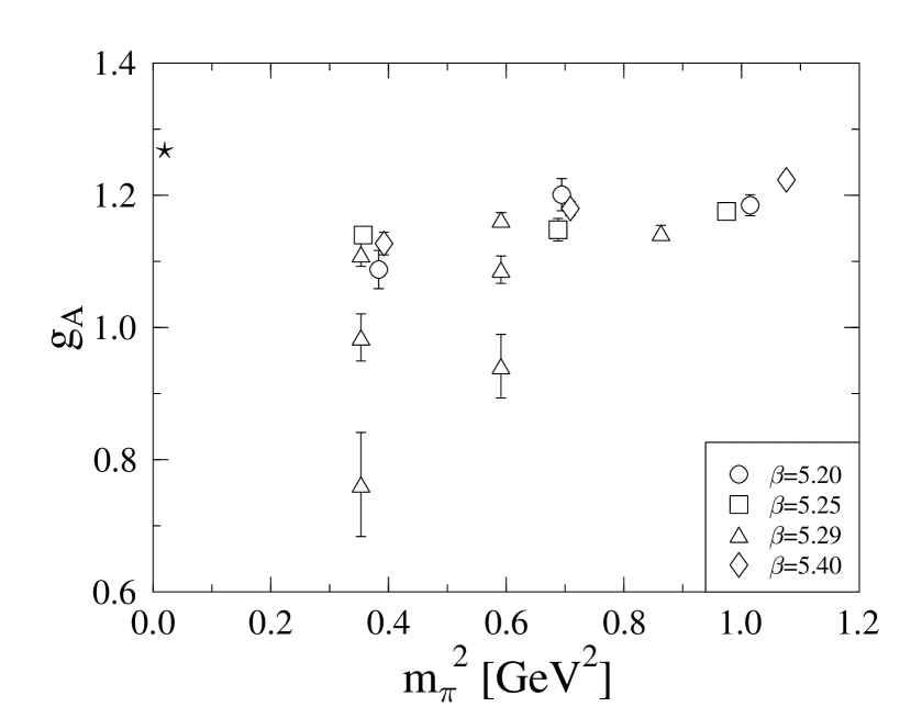
Figure 32: Isovector axial vector coupling constant $g_{A}$ (from [K⁺06]).

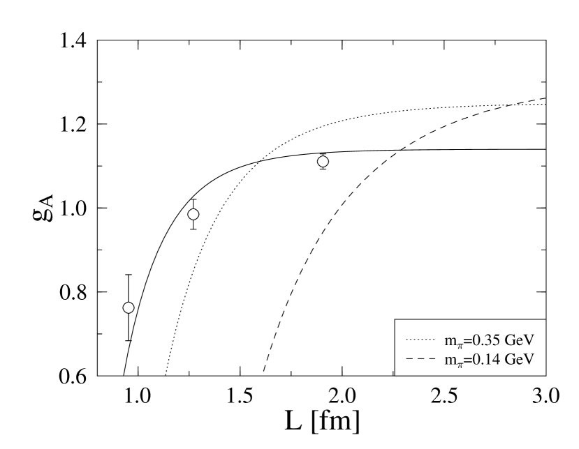
Figure 33: Volume dependence of the isovector axial vector coupling constant $g_{A}$ (from [K⁺06]).

A detailed study of the infinite volume SSE HBChPT extrapolation of $g_{A}$ has been presented in [PMHW07]. From a fit to lattice data points and the experimental value, the convergence pattern of the chiral extrapolation was numerically investigated by a subsequent series expansion in powers of $m_{\pi}$. As displayed in Fig. 34, the chiral expansion in $m_{\pi}$ slowly converges only for pion masses below $\approx\text{{\small$\Delta$}}m_{\Delta N}\approx 300\text{ MeV}$. This indicates that systematic uncertainties in a conventional HBChPT extrapolation of $g_{A}$, where explicit $\Delta$-DOFs have been integrated out and are only included in the form of LECs (couplings) at higher orders in the chiral Lagrangian, may be substantial above $m_{\pi}\approx 300\text{ MeV}$. An explicit, “non-perturbative” inclusion of the $\Delta$-resonance appears to be crucial for $g_{A}$.

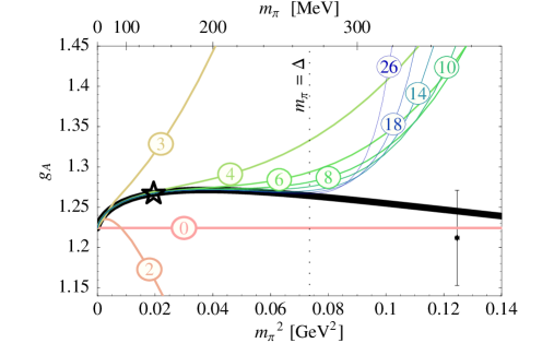
Figure 34: Study of the convergence pattern of the SSE HBChPT extrapolation of $g_{A}$ to $\mathcal{O}(\epsilon^{3})$ in infinite volume (from [PMHW07]). The numbers $n=0,2,3,4,\ldots$ represent the orders at which the expansion in $m_{\pi}$ was truncated.

The results from QCDSF/UKQCD are in overall agreement with calculations performed by LHPC based on the hybrid approach of domain wall valence and Asqtad sea quarks [E⁺06a], as can be seen from Fig. 36, where the uncorrected, “large” volume results from Fig. 33 are presented by the upwards pointing triangles. In particular for $m_{\pi}\approx 600\text{ MeV}$, the QCDSF/UKQCD data points, corresponding to volumes of $V\approx(1.5,\ldots,2\text{ fm})^{3}$, would be slightly shifted upwards by finite volume corrections, and therefore agree within statistics with the LHPC results, which have been obtained for $V\approx(2.5\text{ fm})^{3}$ ($V\approx(3.5\text{ fm})^{3}$ for the leftmost data point in Fig. 36). A chiral fit based on results from HBChPT including explicit $\Delta$-DOFs in a finite volume [BS04] (very similar to the SSE HBChPT calculation discussed above) to the LHPC lattice data given by the filled squares is shown in Fig. 36 as shaded band. Finite volume corrections were found to be small and negligible within statistical errors, as can also be inferred directly from the two leftmost data points in Fig. 36 that were obtained for $V\approx(2.5\text{ fm})^{3}$ and $V\approx(3.5\text{ fm})^{3}$, respectively. This is in agreement with the results presented in Fig. 33, which point towards small finite volume corrections for $L\geq 2.5\text{ fm}$ even for the lowest accessible pion masses of $m_{\pi}\approx 350\text{ MeV}$, i.e. for $m_{\pi}L\gtrapprox 4.5$. The infinite volume chiral extrapolation based on the LHPC results in Fig. 36 is found to be in good agreement with the experimental value within errors.

A somewhat different point of view concerning finite volume corrections to $g_{A}$ is expressed in [Y⁺08] on the basis of recent results obtained for $n_{f}=2+1$ flavors of domain wall fermions displayed in Fig. 38. It has been noted in particular that the lattice data point for the lowest pion mass of $m_{\pi}\approx 330\text{ MeV}$ for $V\approx(2.7\text{ fm})^{3}$ in Fig. 38 lies $\approx 10\%$ lower than the results at $m_{\pi}\approx 420\text{ MeV}$ as well as the results from LHPC (denoted by “$N_{f}=2+1$ Mix”) at $m_{\pi}\approx 350\text{ MeV}$. Motivated by the empirical observation that the volume dependence of a number of results for $g_{A}$ from different groups can be approximately described in terms of the single variable $m_{\pi}L$, an ansatz of the form $A+Bm_{\pi}^{2}+C\exp(-m_{\pi}L)$ has been used to simultaneously fit the volume and pion mass dependence of the lattice data. Results of such fits are shown by the dashed lines in Fig. 38 for the volumes $V\approx(2.7\text{ fm})^{3}$ and $V\approx(1.8\text{ fm})^{3}$. These phenomenological fits indeed suggest the presence of significant finite volume corrections in the relevant region of $m_{\pi}\approx 330,\ldots,360\text{ MeV}$ and for volumes of $V<(3\text{ fm})^{3}$, in contradiction to the SSE HBChPT results discussed above, as shown in particular in Fig. 33. It may, however, be noted noted that the low-lying, leftmost lattice data point in Fig. 38 has been obtained from a central average over the somewhat asymmetric plateau in the ratio of three- to two-point functions displayed on the top in Fig. 38. Due to the asymmetrically distributed data points around $t=6$, the choice of the plateau region is a potential source of an additional systematic uncertainty. If included, it may reduce the statistical significance of the observed difference to the other lattice data points at $m_{\pi}\approx 350\text{ MeV}$ and $m_{\pi}\approx 420\text{ MeV}$ in Fig. 38.

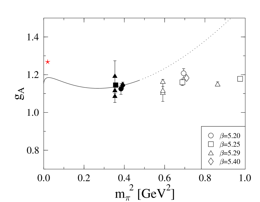
Figure 35: Isovector axial vector coupling constant $g_{A}$ (from [K⁺06]).

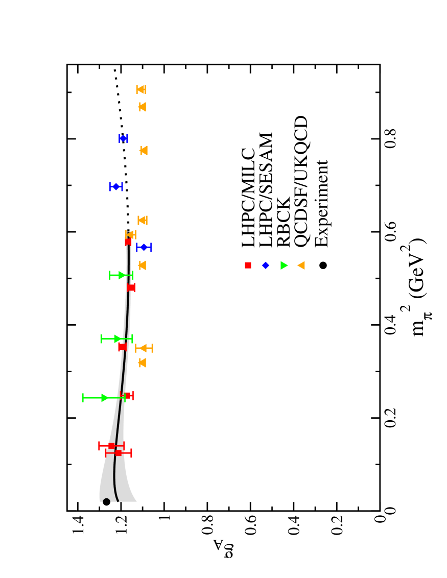
Figure 36: Isovector axial vector coupling constant $g_{A}$ [E⁺06a] compared to results from QCDSF/UKQCD [K⁺06], LHPC/SESAM [D⁺02] and RBC [OO05] (figure from [E⁺06a]).

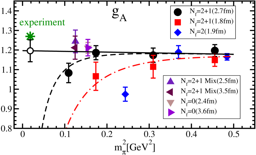
Figure 37: Isovector axial vector coupling constant $g_{A}$ (from [Y⁺08]).

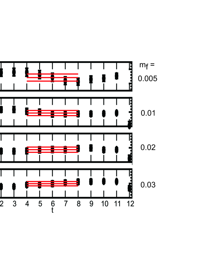
Figure 38: Plateaus for $g_{A}$ (from [Y⁺08]).

3.4.5 Tensor form factors and tensor charge

As before, all results discussed in this section have been obtained for non-perturbatively renormalized operators and are given in the $\overline{\text{MS}}$ scheme at a renormalization scale of $\mu=2\text{ GeV}$, unless stated otherwise. For details, we refer to the original works.

An overview of lattice results from QCDSF/UKQCD for the tensor form factor $G_{T}(t=-Q^{2})=A_{T10}(t=-Q^{2})$ for up- and down-quarks is given Fig. 39, obtained for pion masses of $m_{\pi}\approx 600,\ldots,1200\text{ MeV}$, lattice spacings of $a\approx 0.07,\ldots,0.11\text{ fm}$ and volumes of $V\approx(1.4,\ldots,2.0\text{ fm})^{3}$ [G⁺05g]. Contributions from disconnected diagrams, which would only drop out in the isovector channel, were not included. However, since the underlying tensor operator $\overline{q}i\sigma^{\mu\nu}q$ flips the helicity of the quarks, the disconnected contributions will not contribute in the combined continuum and chiral limit, $(a,m_{q})\rightarrow 0$, and are expected to be suppressed even at finite quark masses. The lattice data points in Fig. 39 have already been extrapolated to the continuum limit and the physical pion mass by means of a simultaneous global fit to the full $Q^{2}$-, $m_{\pi}$- and $a$-dependence, including all available ensembles. A dipole ansatz of the form

$$A_{T10}^{\text{dipole},m_{\pi},a}(t)=\frac{A_{T10}^{0}(0)+\alpha_{1}m_{\pi}^{2}+\alpha_{2}a^{2}}{\left(1-\frac{t}{(m_{D}^{0}+\alpha_{3}m_{\pi}^{2})^{2}}\right)^{2}}\ ,$$ (139)

with five fit parameters $A_{T10}^{0}(0)$, $m_{D}^{0}$ and $\alpha_{1},\ldots,\alpha_{3}$, where the $\alpha_{i}$ describe the lattice spacing and $m_{\pi}^{2}$-dependence of the forward value and the dipole mass, has been fitted to the lattice data points. In a second step, the fit result was used to shift the original data points to the continuum limit and the physical pion mass by subtracting the difference $A_{T10}^{\text{dipole},m_{\pi}^{\text{latt}},a}(t)-A_{T10}^{\text{dipole},m_{\pi}^{\text{phys}},a=0}(t)$.

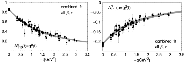
Figure 39: Tensor form factor $G_{T}(t=Q^{2})=A_{T10}(t=Q^{2})$ (from [G⁺05g]).

The overall agreement of the shifted data points in Fig. 39 shows that this simplistic treatment of the $Q^{2}$-, $m_{\pi}$- and $a$-dependence works surprisingly well, but clearly a more sophisticated approach will be necessary in the case that lattice data at lower pion masses is included. From the global simultaneous fit, a tensor charge of $g^{u}_{T}=A^{u}_{T10}(Q^{2}=0)=0.857(13)$ for up-, and $g^{d}_{T}=A^{d}_{T10}(Q^{2}=0)=-0.212(05)$ for down-quarks was found. This agrees within statistical errors with the results from a separate linear chiral extrapolation of $g^{u}_{T}$ and $g^{d}_{T}$, as plotted in Fig. 40. The $m_{\pi}^{2}$-dependence of the tensor charge is indeed to a very good approximation linear and almost flat over the whole range of accessible pion masses. We also quote the values for the dipole masses obtained from the fit using Eq. 139, which are $m^{u}_{D}=1.732(36)\text{ GeV}$ $m^{d}_{D}=1.741(56)\text{ GeV}$ at the physical pion mass. This translates into mean square tensor charge radii of $\langle r_{T}^{2}\rangle_{u}=0.156(7)\text{ fm}^{2}$ and $\langle r_{T}^{2}\rangle_{d}=0.154(10)\text{ fm}^{2}$, which are in the same ballpark as the (isovector) axial-vector radius $\langle r_{A}^{2}\rangle_{u-d}$ in Fig. 29, but clearly smaller than the isovector Dirac radius $\langle r_{1}^{2}\rangle_{u-d}$ in Fig. 20.

Results for the isovector tensor charge from RBC for $n_{f}=2$ flavors of domain wall fermions are displayed in Fig. 42 [LBO⁺08]. Clearly, the results for the three different pion masses with $m_{\pi}>490\text{ MeV}$ do not allow for a systematic extrapolation to the physical point, so that the value of $g^{u-d}_{T}=0.93(6)$ obtained from a linear extrapolation in $m_{\pi}^{2}$ should, in the best case, be seen as indicative. Figure 42 shows $g^{u-d}_{T}$ as obtained more recently by RBC-UKQCD in the framework of simulations with $n_{f}=2+1$ flavors of domain wall fermions [OY08] for pion masses between $\approx 331$ and $\approx 672\text{ MeV}$. The low value of the tensor charge at the smallest pion mass may be an indication for finite volume effects. Overall agreement is observed for the $n_{f}=2$ and $n_{f}=2+1$ results in Fig. 42 and Fig. 42, respectively, which in both cases were non-perturbatively renormalized and are given in the $\overline{\text{MS}}$ scheme at a scale of $\mu=2\text{ GeV}$.

Based on the hybrid approach of $n_{f}=2+1$ domain wall valence Asqtad staggered sea quarks, LPHC has computed the isovector tensor charge for pion masses in the range of $\approx 350\text{ MeV}$ to $\approx 760\text{ MeV}$, as displayed in Fig. 43 [E⁺06b]. In contrast to the corresponding study of the axial-vector operator discussed in section 3.4.4, the tensor operator, $\overline{q}i\sigma^{\mu\nu}q$, has in this case been renormalized and transformed to the $\overline{\text{MS}}$ scheme at a scale of $\mu=2\text{ GeV}$ using a non-perturbatively (NP-) improved perturbative renormalization constant,

$$Z_{\mathcal{O}}=Z_{\mathcal{O}}^{\text{PT}}\frac{Z_{A}^{\text{NPT}}}{Z_{A}^{\text{PT}}}\,,$$ (140)

with $\mathcal{O}=\mathcal{O}_{T}$, employing the non-perturbative axial-vector renormalization constant $Z_{A}^{\text{NPT}}$ in combination with $Z_{\mathcal{O}}^{\text{PT}}$ and $Z_{A}^{\text{PT}}$ obtained from 1-loop lattice perturbation theory [Bis05]. We note that although the perturbative renormalization constants are already close to unity due to HYP-smearing of the gauge fields, it is not guaranteed that the NP-improved renormalization factors in Eq. 140 agree within statistical errors with the (at this point unknown) fully non-perturbative renormalization factors. This potential systematic uncertainty should be kept in mind when comparing the lattice data from the mixed-action approach by LHPC, e.g. in Fig. 43, to other simulation results.

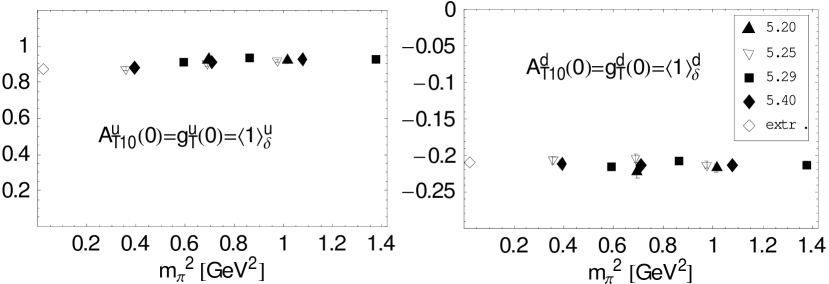
Figure 40: Tensor charge $g_{T}$ versus $m_{\pi}^{2}$ (from [G⁺05g]).

The shaded band in Fig. 43 represents a chiral extrapolation of the lattice data points based on a self-consistent rearrangement of the leading 1-loop HBChPT formula [AS02, CJ01], given by [E⁺06b]

$$g_{T}=\langle 1\rangle_{\delta u-\delta d} = \delta g_{T}^{0}\left(1-\frac{(4g_{A,\text{lat}}^{2}+1)}{2(4\pi)^{2}}\frac{m_{\pi,\text{lat}}^{2}}{f_{\pi,\text{lat}}^{2}}\ln\left(\frac{m_{\pi,\text{lat}}^{2}}{f_{\pi,\text{lat}}^{2}}\right)\right)+\delta c_{0}\frac{m_{\pi,\text{lat}}^{2}}{f_{\pi,\text{lat}}^{2}}\,,$$ (141)

where the LECs in the chiral limit have been replaced by the respective pion mass dependent values $g_{A,\text{lat}}$ and $f_{\pi,\text{lat}}$ obtained in the lattice calculation. Although chiral extrapolations based on self-consistently improved ChPT have shown some success in the extrapolation to the physical point and comparison with experimental results [E⁺06b], it is difficult to judge if the extrapolation in Fig. 43 describes the underlying physics correctly. After all, such a rearrangement of the chiral series cannot possibly account for all analytic and non-analytic structures in $m_{\pi}$ that are in principle relevant at the currently accessible pion masses. A value of $g_{T}=\langle 1\rangle_{\delta u-\delta d}\approx 0.82(2)$ is found at the physical ratio $m_{\pi,\text{phys}}^{2}/f_{\pi,\text{phys}}^{2}\approx 2.4$.

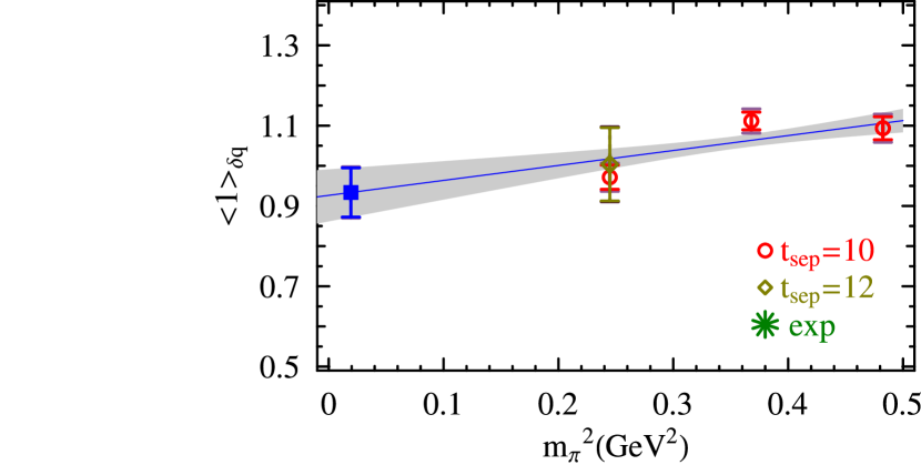
Figure 41: Pion mass dependence of the isovector tensor charge $g_{T}$ (from [LBO⁺08]).

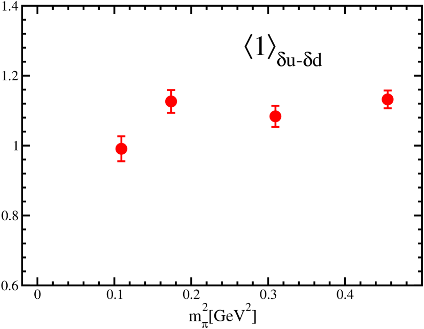
Figure 42: Pion mass dependence of the isovector tensor charge $g_{T}$ (from proceedings [OY08]).

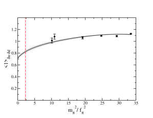
Figure 43: Pion mass dependence of the isovector tensor charge $g_{T}$ (from proceedings [E⁺06b]).

Lattice results for the nucleon tensor form factor $\overline{B}_{T10}(Q^{2})$ are particularly relevant for an understanding of the transverse nucleon spin structure, as explained in section 2.1.6, and will be discussed in relation with transverse spin densities of quarks in the nucleon in section 4.4.6 below.

3.5 Electromagnetic form factors of the $\rho$-meson

A first preliminary computation of the form factor $G_{1}(Q^{2})$ of the $\rho$-meson in unquenched lattice QCD has been performed using so-called density-density correlators [AK07] (for a very recent study by the same authors of hadron deformations using density-density correlators, we refer to [AK08] and section 6.0.1 below). For the case of the $\rho$-meson one considers four-point functions of the form

$$C^{\mu\nu}_{\text{4pt}}(\mathbf{x},t_{1},t_{2}) = \int d^{3}x_{1}d^{3}x_{2}\langle\rho(\mathbf{x}_{2},t)|J^{\mu}_{u}(\mathbf{x}+\mathbf{x}_{1},t_{2})J^{\nu}_{d}(\mathbf{x}_{1},t_{1})|\rho(\mathbf{x}_{0},t_{0})\rangle\,.$$ (142)

Fourier-transforming this with respect to $\mathbf{x}$, inserting of a complete set of states, and using isospin symmetry, one finds for e.g. $\mu=\nu=4$ at large time-distances $t_{2}-t_{1},t-t_{0},t-t_{2}\gg 0$ that $C^{44}_{\text{4pt}}(\mathbf{P},t_{1},t_{2})\propto e^{(-E_{\rho}(\mathbf{P})(t_{2}-t_{1}))}e^{(-E_{\rho}(\mathbf{P}^{\prime})(t-(t_{2}-t_{1})-t_{0}))}G_{1}(Q^{2})^{2}$, where $\mathbf{P}^{\prime}=0$, $Q^{2}=-(P-P^{\prime})^{2}$, from which the (squared) form factor $G_{1}(Q^{2})$ can be extracted by taking appropriate ratios with $\rho$-meson two-point-functions. Because of the integrals over $x_{1}$ and $x_{2}$ in Eq. (142), the evaluation of the 4-point correlator requires in general all-to-all propagators. It has been shown in [AK07] how the one-end trick that has already been successfully used for the calculation of pion correlators (see section 2.3.3 above) can also be used for the evaluation of the four-point functions of the $\rho$-meson, leading to a substantial reduction of the stochastic noise compared to the standard method using all-to-all propagators. Gaussian smearing, combined with HYP-smearing, of the interpolating source and sink fields was shown to be crucial to suppress contaminations from excited states. Using these methods, calculations have been performed for $n_{f}=2$ flavors of Wilson fermions and the Wilson gauge action, for pion masses of $\approx 384$, $\approx 510$ and $\approx 690\text{ MeV}$, a lattice spacing of $a\approx 0.08\text{ fm}$ and a volume of $V\approx(1.9\text{ fm})^{3}$. The results for the $\rho$-meson form factor $G_{1}(Q^{2})$ are displayed in Fig. 45, showing a very good precision over a wide range of $Q^{2}$. Keeping in mind the exploratory character of this calculation, the results in Fig. 45 seem already to indicate that the slope in $Q^{2}$, and therefore the charge radius, is increasing for decreasing pion mass.

Figure 44: $G_{1}$ of the $\rho$-meson as a function of the momentum transfer $Q^{2}$ for three $\kappa$ values (from proceedings [AK07]).

Figure 45: Pion mass dependence of the $\rho$-meson charge radius in the quenched approximation, compared to corresponding up- and strange-quark contributions to the $K^{*}$ charge radius (from [H⁺07b]).

An extensive study of the charge radii, magnetic and quadrupole moments of the $\rho$ and the $K^{*}$ mesons in quenched lattice QCD has been presented recently, based on fat-link irrelevant clover (FLIC) improved Wilson fermions and an $\mathcal{O}(a^{2})$ improved gauge action [H⁺07b]. Results have been obtained for a lattice spacing of $a\approx 0.128\text{ fm}$ in a volume of $V\approx(2.6\text{ fm})^{3}$, with pion masses as low as $\approx 300\text{ MeV}$. The local vector current has been renormalized by demanding charge conservation, i.e. $G_{C}(Q^{2}\text{{=}}0)=1$. Since the analysis has been restricted to a single non-zero $Q^{2}\approx 0.22\text{ GeV}^{2}$, it was assumed in the extraction of the magnetic moment $\mu=G_{M}(0)$ that the magnetic and charge form factors scale identically at small $Q^{2}$, such that $\mu_{\rho}=G_{M}(0)\simeq G_{M}(0.22\text{ GeV}^{2})/G_{C}(0.22\text{ GeV}^{2})$. For the same reason, the mean square charge radius was calculated from $\langle r^{2}\rangle=6(G_{C}(Q^{2})^{-1}-1)/Q^{2}$ for $Q^{2}\approx 0.22\text{ GeV}^{2}$, corresponding to a monopole ansatz for the $Q^{2}$-dependence of $G_{C}(Q^{2})$. Results for the charge radius of the $\rho$-meson as a function of the pion mass are shown in Fig. 45. As before, the charge radius is increasing at lower pion masses, with a value of $\langle r_{\rho}^{2}\rangle=0.546(97)\text{ fm}^{2}$ at $m_{\pi}\approx 300\text{ MeV}$. Figure 47 displays the magnetic moment in natural magnetons (also called the $g$-factor), which is approximately constant as a function of $m_{\pi}^{2}$. A value of $g_{\rho}=\mu_{\rho}=2.21(15)$ was obtained at the lowest accessible pion mass of $\approx 300\text{ MeV}$. The pion mass dependence of the $\rho$-meson quadrupole form factor $G_{Q}(Q^{2})$ at $Q^{2}\approx 0.22\text{ GeV}^{2}$ is displayed in Fig. 47. A small negative value of $G_{Q}(Q^{2}\approx 0.22\text{ GeV}^{2})=-0.0050(27)\text{ fm}^{2}$ was found at $m_{\pi}\approx 300\text{ MeV}$. Although the statistical errors are rather large, these results give a first indication that the charge distribution of the $\rho$-meson is oblate.

Figure 46: Pion mass dependence of the $\rho$-meson magnetic moment in natural units (g-factor) obtained from $\mu_{\rho}=G_{M}(0)\widetilde{=}G_{M}(0.22\text{ GeV}^{2})/G_{C}(0.22\text{ GeV}^{2})$ in the quenched approximation (from [H⁺07b]).

Figure 47: Pion mass dependence of the $\rho$-meson quadrupole moment in the quenched approximation (from [H⁺07b]).

First preliminary results for the electromagnetic form factors of the rho in unquenched lattice QCD, based on standard two- and three-point functions, have recently been obtained by QCDSF/UKQCD [G⁺08d]. Calculations have been performed for a set of ensembles for $n_{f}=2$ flavors of Wilson fermions, as described in the previous sections. Figure 49 shows the charge, magnetic and quadrupole form factors as functions of the momentum transfer squared for a pion mass of $\approx 400\text{ MeV}$ in a volume of $V\approx(1.8\text{ fm})^{3}$. The local vector current has been renormalized such that $G_{C}(Q^{2}=0)=1$. Monopole, dipole, and linear fits to $G_{C}(Q^{2})$, $G_{M}(Q^{2})$ and $G_{Q}(Q^{2})$, respectively, are represented by the shaded bands in Fig. 49. While the quality of the lattice data for $G_{C}(Q^{2})$ is very good, the results for $G_{M}(Q^{2})$ in particular show some scatter. Many of the lattice data points for the quadrupole form factor are compatible with zero within errors, but there is a general trend towards negative values at lower $Q^{2}$, indicating a non-spherical charge distribution within the rho. Since the mass of the $\rho$-meson is in this case close to or even slightly above the two-pion threshold, $m_{\rho}\gtrapprox 2m_{\pi}$, these results have to be considered with greatest care. For a related preliminary study of the $\rho$-meson mass from a phase-shift analysis in finite volume, performed in the same simulation framework, we refer to [G⁺08b]. The pion mass dependence of the charge radius, which has been obtained from monopole fits to the lattice data, is displayed in Fig. 49. From a linear interpolation in $m_{\pi}^{2}$, a value of $\langle r_{\rho}^{2}\rangle=0.46(3)\text{ fm}^{2}$ was found at $m_{\pi}\approx 450\text{ MeV}$. The magnetic moment has been obtained from an extrapolation of $G_{M}(Q^{2})$ to $Q^{2}=0$ using a dipole parametrization as shown in Fig. 49, and the results for $\mu_{\rho}$ as a function of $m_{\pi}^{2}$ are presented in Fig. 51. Within statistical errors, $\mu_{\rho}$ is approximately independent of the pion mass, and we note that the central values are somewhat below the results from [H⁺07b] displayed in Fig. 47. The linear interpolation in $m_{\pi}^{2}$ gives $\mu_{\rho}=1.69(10)$ at $m_{\pi}\approx 450\text{ MeV}$, which is $\approx 25\%$ below the corresponding values in Fig. 47. Further studies are necessary to see if this is related to the quenched approximation or the ansatz $\mu_{\rho}=G_{M}(0)\simeq G_{M}(0.22\text{ GeV}^{2})/G_{C}(0.22\text{ GeV}^{2})$ used in [H⁺07b], or any other systematic uncertainties affecting the unquenched results in Fig. 49. Results for the quadrupole moment, $Q_{\rho}=G_{Q}(Q^{2}=0)/m_{\rho}^{2}$, which have been obtained from linear extrapolations to $Q^{2}=0$, are presented in Fig. 51 versus the pion mass squared.

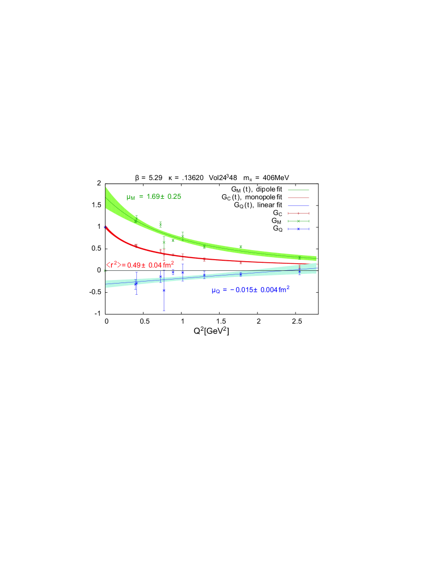
Figure 48: Electromagnetic form factors of the rho meson (from proceedings [G⁺08d]).

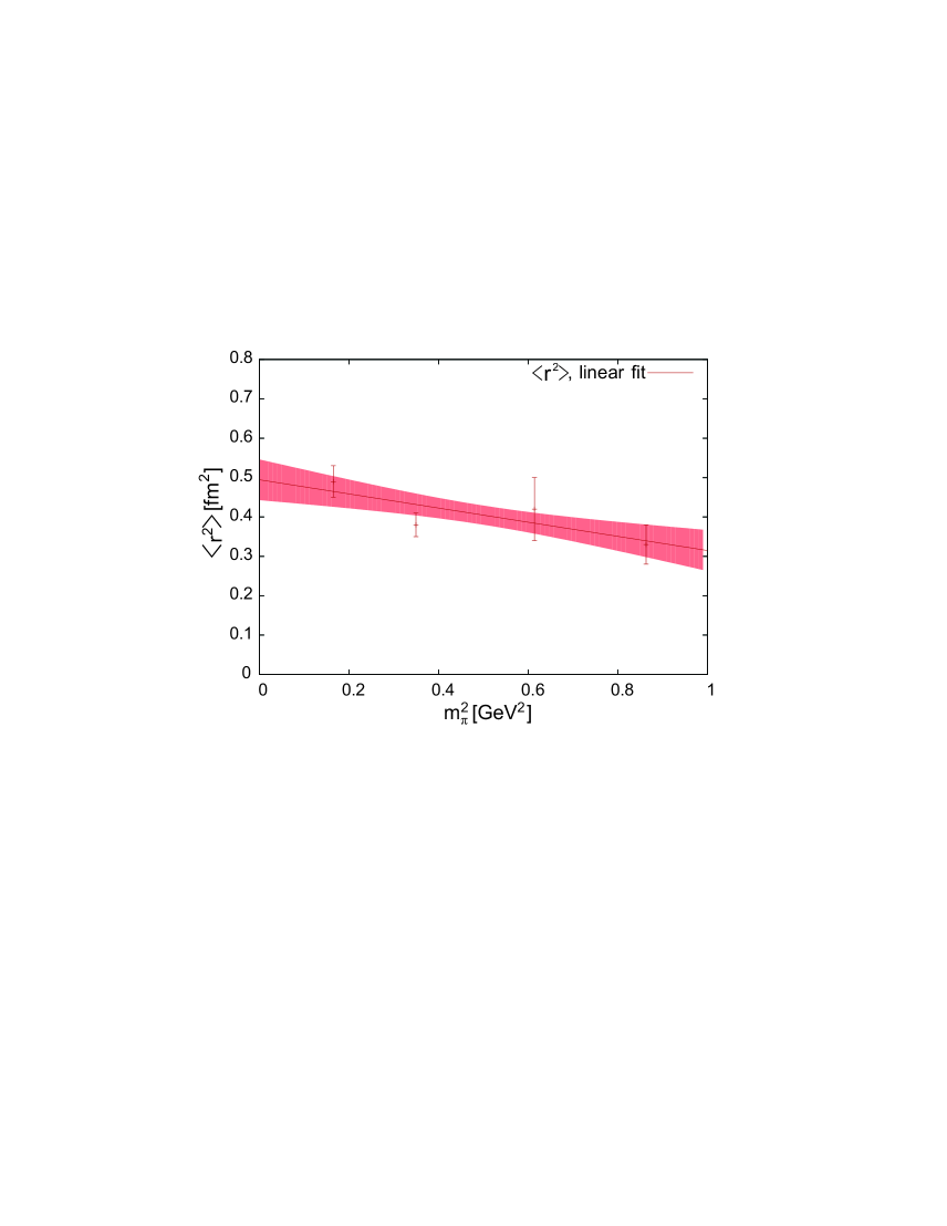
Figure 49: Pion mass dependence of the rho charge radius (from proceedings [G⁺08d]).

While the results at larger $m_{\pi}$ are compatible with zero within errors, a non-zero, negative value of $Q_{\rho}=-0.0125(15)\text{ fm}^{2}$ at $m_{\pi}\approx 450\text{ MeV}$ was obtained from a linear interpolation shown by the shaded band in Fig. 51. This is approximately a factor of two to three larger than the values in Fig. 47 above for $G_{Q}(Q^{2}\approx 0.22\text{ GeV}^{2})$ obtained in the quenched approximation. In summary, to this date all lattice QCD calculations of the quadrupole form factor of the $\rho$-meson give a non-zero and negative quadrupole moment $Q_{\rho}$, indicating that the charge distribution of the rho is oblate. Further improved studies of the form factors and critical analyses of the employed assumptions and extrapolations are certainly required for a better understanding of the systematic errors and in order to confirm these interesting preliminary results.

A study of the magnetic moment of spin-1 mesons using the background field method (purely based on hadron two-point functions) has been presented recently in [LMW08]. For a brief introduction to the background field method and the extraction of, e.g., magnetic moments from mass shifts we refer to section 3.7. Calculations were performed in the quenched approximation using Wilson fermions and the Wilson gauge action for pion masses ranging from $\approx 522\text{ MeV}$ to $\approx 1015\text{ MeV}$, a lattice spacing of $a\approx 0.1\text{ fm}$ and a volume of $V\approx(2.4\text{ fm})^{3}$. The values for the $g$-factor of the $\rho$-meson ($\mu_{\rho}$ in natural units) obtained in this study are in remarkably good agreement with the values from the conventional approach based on three-point functions display in Fig. 47 that were also calculated in the quenched approximation. It is encouraging to see that the two very different methods lead to such consistent results.

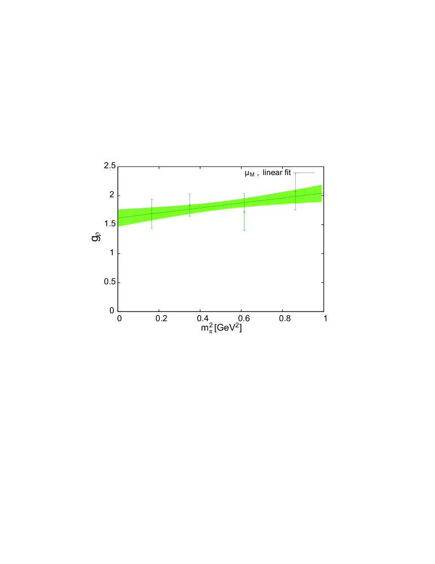
Figure 50: Pion mass dependence of the rho magnetic moment (from proceedings [G⁺08d]).

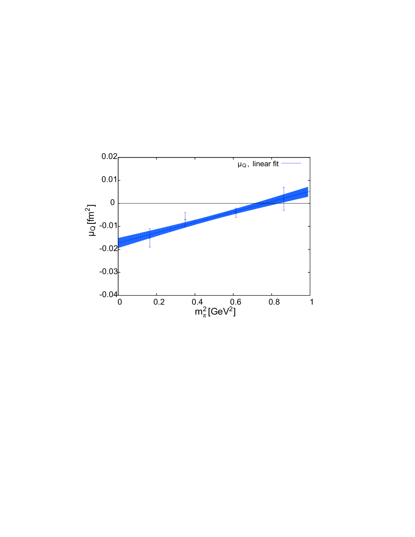
Figure 51: Pion mass dependence of the rho quadrupole moment (from proceedings [G⁺08d]).

3.6 Form factors of the $\Delta$-baryon

An extensive first study of the form factors of the decuplet baryons in quenched lattice QCD was published already in the early 1990’s [LDW92]. The calculations were performed for two values of the momentum transfer $Q^{2}=0$ and $Q^{2}\approx 0.16\text{ GeV}^{2}$, for three different pion masses, on a $24\times 12\times 12\times 24$ lattice, with a lattice spacing of $a\approx 0.128\text{ fm}$. Without going into the details of this early study, we mention here only that results were obtained for the charge radius, magnetic moment, quadrupole and octupole form factor in particular of the $\Delta$-resonance. From linear chiral extrapolations, values for the mean square charge radius of $\langle r_{\Delta}^{2}\rangle=0.393(90)\text{ fm}^{2}$, and for the magnetic form factor of $G^{\Delta^{+}}_{M1}(0.16\text{ GeV}^{2})=2.22(44)$ were obtained for, e.g., the $\Delta^{+}$. The central values of the quadrupole, $G^{\Delta^{+}}_{E2}$, and octupole, $G^{\Delta^{+}}_{M3}$, form factors at $Q^{2}=0.16\text{ GeV}^{2}$ were found to be negative and positive, respectively, but in both cases compatible with zero within statistical errors.

Results for the magnetic moment of the $\Delta^{+}$-baryon from a more recent study in quenched lattice QCD using FLIC fermions (with same lattice parameters as in the study of the $\rho$-meson discussed in the previous section) [B⁺06b] are displayed in Fig. 53 as a function of $m_{\pi}^{2}$, with a value of $\mu_{\Delta^{+}}\approx 1.80(15)$ in units of nuclear magnetons at a pion mass of $\approx 372\text{ MeV}$. Notably, the sign of the curvature for the proton and for the $\Delta^{+}$-state are opposite at lower pion masses. This may be understood in the framework of ChPT, where it has been shown that contributions to $\Delta$-decay that become increasingly important as one approaches the $\Delta\rightarrow N\pi$ threshold, have opposite signs in full QCD and QCD in the quenched approximation [LS96, L⁺04]. The different pion mass dependences of the proton and $\Delta$-baryon magnetic moments in Fig. 53 have therefore been interpreted as clear signature of the quenched approximation [L⁺04]. This “quenched oddity” [LS96] is interesting by itself but clearly makes a comparison of lattice results with experimental data in this channel even more delicate if not impossible.

Magnetic moments of baryons, specifically the $\Delta$ states, were also studied in quenched QCD using the background field method (see section 3.7 below) [LKZW05]. The calculations were based on the Wilson gauge and fermion actions, with a lattice spacing of $a\approx 0.1\text{ fm}$ for a volume of $\approx(2.4\text{ fm})^{3}$ and pion masses in the range of $\approx 520\text{ MeV}$ to $\approx 1010\text{ MeV}$. Quantization conditions for the external magnetic fields were not considered, and it was attempted to keep the boundary effects small by using Dirichlet boundary conditions, small values of the external fields, and by placing the sources centrally in the spatial direction. Four different values of the magnetic field $B$ for the up- and down-quarks were employed in the calculation of the two point functions, and even-power terms in the expansion Eq. 143 were eliminated by also computing the mass shifts $\Delta E$ for the corresponding negative values, $-B$, and then extracting the magnetic moments from $(\Delta E(B)-\Delta E(-B))/2$. The results for the magnetic moments in natural units were first converted to nuclear magnetons with factors of $m_{N}^{\text{phys}}/m^{\text{lat}}_{h}$, where $m^{\text{lat}}_{h}$ is the pion mass dependent hadron mass measured on the lattice, and then extrapolated to $m^{\text{phys}}_{\pi}$ using different ansätze for the pion mass dependence. Extrapolations linear in $m_{\pi}$ gave results for the baryon octet magnetic moments and the $\Delta^{++}$-baryon that were $\approx 10\%$ to $\approx 25\%$ above the experiment (in terms of absolute values), with the exception of the neutron magnetic moment, which came out slightly below the experimental result. The pion mass dependence of the proton and $\Delta^{+}$ magnetic moments turns out to be well compatible with the results in Fig. 53, and the central values obtained in [LKZW05] using the background field method are only slightly above the values from the standard form factor calculation of [BLW⁺06]. To study possible finite size effects, the background-field calculations were repeated for a smaller volume of $V\approx(1.6\text{ fm})^{3}$. The absolute values for the proton and neutron magnetic moment came out significantly lower than for the larger volume, even for large pion masses. This may indicate that effects from the boundary, due to abandoning the quantization condition and using Dirichlet boundary conditions, may be non-negligible and affect the results even in the larger volume.

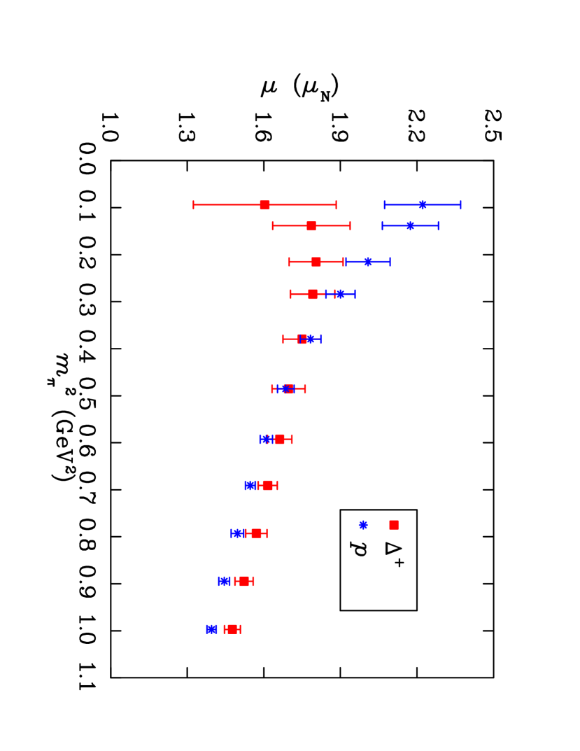
Figure 52: Pion mass dependence of the $\Delta^{+}$ magnetic moment in the quenched approximation (from proceedings [BLW⁺06]).

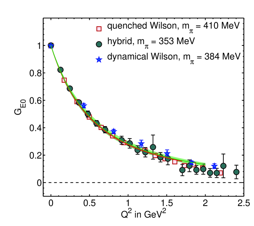
Figure 53: Connected contributions to the electric charge form factor of the $\Delta^{+}$-baryon (from [A⁺09a]).

An extensive study of the form factors of the $\Delta$-baryon for a much larger range of values of the momentum transfer squared, $Q^{2}=0,\ldots,2.25\text{ GeV}^{2}$, in quenched and unquenched lattice QCD was presented recently [A⁺09a]. Here we will concentrate on a discussion of the unquenched results. Calculations were performed using $n_{f}=2$ flavors of Wilson fermions and the Wilson gauge action for a lattice spacing of $a\approx 0.077\text{ fm}$ in a volume of $V\approx(1.85\text{ fm})^{3}$, for three values of the pion mass ranging from $\approx 384\text{ MeV}$ to $\approx 691\text{ MeV}$. Further results were obtained in the framework of the mixed action approach with $n_{f}=2+1$ flavors of DW valence fermions and Asqtad staggered sea quarks (using MILC configurations), for a lattice spacing of $a\approx 0.124\text{ fm}$, a volume of $V\approx(3.5\text{ fm})^{3}$, and a pion mass of $m_{\pi}\approx 353\text{ MeV}$. The analysis was based on a standard ratio of $\Delta^{+}$-three- to two-point functions, where the three-point functions were calculated using the sequential source technique with the sink momentum set to zero. In this study, the (local) charge weighted electromagnetic current, $J_{EM}^{\mu}=\sum_{q=u,d}e_{q}\overline{q}\gamma^{\mu}q$, was employed, and we note that only contributions from quark line connected diagrams were included. As usual, the current operator was renormalized such that $G^{\Delta^{+}}_{E0}(0)=1$. The $Q^{2}$-dependence of the electric charge form factor $G^{\Delta^{+}}_{E0}(Q^{2})$ is displayed in Fig. 53 for the lowest accessible pion masses, showing a very good precision of the lattice data points. Although the $n_{f}=2$ Wilson data points tend to be a bit higher, overall consistency of the results can be observed within statistical errors. A dipole fit to the $n_{f}=2+1$ mixed action calculation is represented by the lighter shaded error band, from which a mean square radius of $\langle r_{E}^{2}\rangle=0.411(28)\text{ fm}^{2}$ was obtained, compared to $\langle r_{E}^{2}\rangle=0.373(21)\text{ fm}^{2}$ for the $n_{f}=2$ Wilson case, for pion masses indicated in the figure.

Figure 55 shows corresponding results for the magnetic dipole form factor $G^{\Delta^{+}}_{M1}(Q^{2})$, also with quite remarkable statistical precision. In this case, an exponential ansatz, $G^{\Delta^{+}}_{M1}(Q^{2})=G^{\Delta^{+}}_{M1}(0)\exp(-Q^{2}/\Lambda^{2}_{M1})$, was used to fit the data and extrapolate to $Q^{2}=0$. The pion mass dependence of the resulting magnetic moment, $\mu_{\Delta^{+}}=G^{\Delta^{+}}_{M1}(0)$ transformed to nuclear magnetons by multiplication with a factor $2m^{\text{phys}}_{N}/(2m^{\text{lat}}_{\Delta})$, is displayed in Fig. 55. An extrapolation to the chiral limit based on a relativistic ChPT calculation in the $\delta$-expansion scheme [PV05] is indicated by the curves, clearly showing a cusp at the pion production threshold, $m_{\delta}>m_{N}+m_{\pi}$, where $\mu_{\Delta^{+}}$ acquires an imaginary part. Very good agreement with the central value of the experimental result, represented by the filled square, is found at the physical pion mass. Clearly, this has to be regarded with great caution due to the large errors of the experimental data point, as well as potential systematic uncertainties of the lattice calculation and the chiral extrapolation.

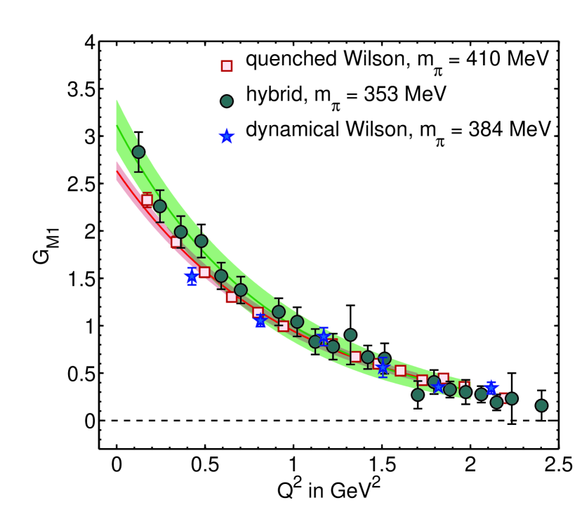
Figure 54: Connected contributions to the magnetic form factor of the $\Delta^{+}$-baryon (from [A⁺09a]).

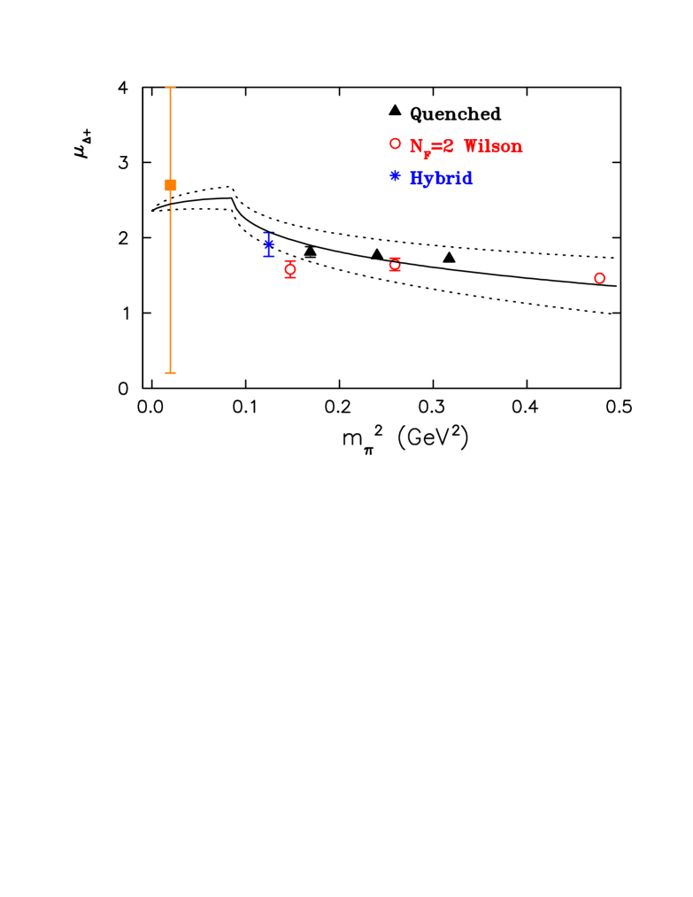
Figure 55: Pion mass dependence of the (real part of the) $\Delta^{+}$ magnetic form factor in units of nuclear magnetons (from [A⁺09a]).

The $Q^{2}$-dependence of the electric quadrupole form factor, $G^{\Delta^{+}}_{E2}(Q^{2})$, is shown in Fig. 57, together with extrapolations based on the exponential ansatz given above. Although the statistical errors are substantial, the data shows a clear trend towards sizeable negative values at $Q^{2}=0$.

A first calculation of the magnetic moments of the $\Delta$-baryons (and the $\Omega^{-}$) using background field methods in full QCD has been presented very recently [AOPV08b]. In this study, the constant external magnetic field, $B$, was implemented using a “patched” electromagnetic potential (or, in a different terminology, including transverse links [DTWL08]) as discussed in section 3.7, leading to the much less restrictive quantization condition $qB=2\pi n/L^{2}$. Calculations were performed for $n_{f}=2+1$ flavors of stout-smeared clover-Wilson fermions on anisotropic lattices with lattice spacings of $a_{t}\approx 0.035\text{ fm}$ and $a_{s}\approx 0.122\text{ fm}$ in temporal and spatial directions, respectively, spatial volumes of $V\approx(1.95\text{ fm})^{3}$ and $V\approx(2.93\text{ fm})^{3}$, and pion masses of $\approx 438\text{ MeV}$ and $\approx 548\text{ MeV}$ for the smaller, and $\approx 366\text{ MeV}$ for the larger volume. For the study of the $\Delta$ magnetic moments, three different $B$-fields, corresponding to $n=\pm 1/2,\pm 1$ and $\pm 2$, were employed. Boundary effects for the choice $n=\pm 1/2$ violating the quantization condition were expected to be negligible [AOPV08b]. Mass differences in the presence of the external magnetic fields were extracted from the $\Delta$- and $\Omega^{-}$-baryon two-point functions, from which the corresponding magnetic moments could be obtained as coefficients of the term linear in $B$, $\Delta m_{h}^{S_{z}}=m_{h}^{S_{z}}(-B)-m_{h}^{S_{z}}(B)=2\hat{S}_{z}B\mu+\mathcal{O}(B^{3})$, where $\hat{S}_{z}=S_{z}/S$ denotes the spin projected in $z$-direction. Comparing the results for the smaller and larger magnetic fields, clear effects from contributions of $\mathcal{O}(B^{3})$ could be observed in particular for larger values of $B$. The data points obtained for the smallest magnetic fields corresponding to $n=\pm 1/2$ were used as final numbers, and shifts from non-vanishing $\mathcal{O}(B^{3})$ terms were estimated to be at most $5\%$. The results for magnetic moment of the $\Delta^{+}$-baryon in units of nuclear magnetons are displayed in Fig. 57 as a function of $m_{\pi}^{2}$, together with the result of a ChPT calculation in the $\delta$-expansion scheme [PV05], represented by the error band. As already noted above with respect to Fig. 55, $\mu_{\Delta^{+}}$ acquires an imaginary part at the $\Delta\rightarrow\pi N$ threshold, i.e. for $m_{\delta}>m_{N}+m_{\pi}$. Comparing the results in Fig. 57 and Fig. 55, we note that the values from the background field calculation are $\approx 25-30\%$ above the data points obtained in the conventional form factor approach based on three-point functions. It would be important to understand the origin of this discrepancy and see if it is, e.g., related to the $Q^{2}$-extrapolation in the form factor calculation, or other systematic uncertainties in these studies. The usual discretization and finite volume effects (not related to the constant magnetic field and boundary effects) in the background field study were estimated to be small, $\approx 3\%$ and $\approx 2\%$, respectively. We note that this study is, in the terminology of [LMW08], “$U(1)$-quenched”, i.e. the constant external magnetic fields were implemented on the level of the valence quarks and the quark propagators, but not in the generation of the gauge configuration, so that the sea quarks effectively carry no electric charges. Effects from a coupling of the sea quarks to the electromagnetic fields were expected to be at most $1\%$. Taking all statistical and estimated systematic uncertainties into account, a value of $\mu_{\Omega^{-}}=-1.93(8)_{\text{stat}}(12)_{\text{sys}}$ in nuclear magnetons was given for the magnetic moment of the $\Omega^{-}$-baryon, obtained directly from a calculation close to the physical strange quark mass. It is encouraging to see that this is in excellent agreement with the average value from the PDG [A⁺08i], $\mu_{\Omega^{-}}=-2.02(5)_{\text{stat+sys}}$.

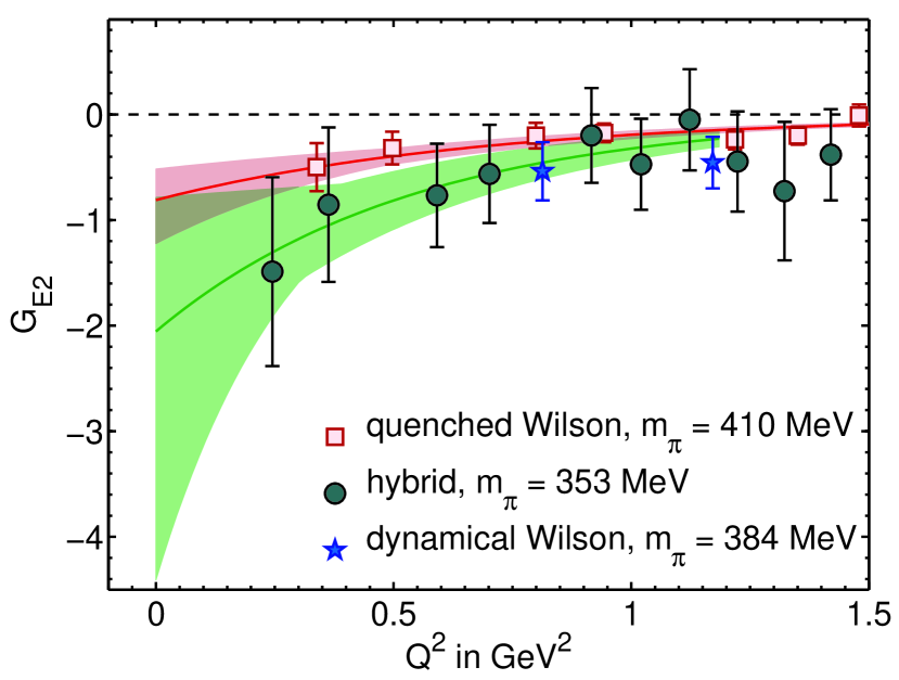
Figure 56: Connected contributions to the quadrupole form factor of the $\Delta^{+}$-baryon (from [A⁺09a]).

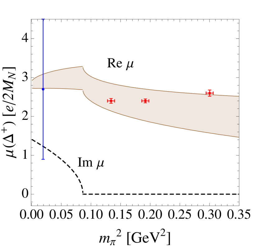
Figure 57: Pion mass dependence of the $\Delta^{+}$ magnetic moment from a background field calculation (from [AOPV08b]).

3.7 Background field methods and static hadron properties

Static quantities like magnetic moments and polarizabilities can be studied using background field methods. Constant electric $\mathbf{E}$ and magnetic $\mathbf{B}$ background fields lead to energy shifts (i.e. shifts in the hadron masses) that can be expanded for small fields,

$$\Delta E=-\mathbf{p}\cdot\mathbf{E}-\boldsymbol{\mu}\cdot\mathbf{B}-\frac{1}{2}\big{(}\alpha_{E}\mathbf{E}^{2}+\beta_{M}\mathbf{B}^{2}\big{)}+\ldots\,,$$ (143)

where the electric and magnetic dipole moments are denoted by $\mathbf{p}$ and $\boldsymbol{\mu}$, respectively, and where $\alpha_{E}$ is the electric, and $\beta_{M}$ is the magnetic polarizability. In a lattice calculation, the mass shifts can be extracted from the exponential decay of the corresponding hadron two-point correlators. Specifically for the magnetic moments $\mu$, background field methods provide an interesting alternative to the standard approach based on hadron three-point functions discussed in the previous sections, where $\mu$ is obtained from an extrapolation of the magnetic form factor to $Q^{2}=0$, $\mu=G_{M}(Q^{2}=0)$. A standard way to couple constant external fields, represented by the electromagnetic potential $A^{EM,\text{ext}}_{\mu}$, to quark fields in the continuum is to use the minimal coupling prescription, i.e. a covariant derivative $D_{\mu}=\partial_{\mu}-igA_{\mu}+ie_{q}A^{EM,\text{ext}}_{\mu}$, where $e_{q}$ is the electric charge of a quark. In the lattice framework, this corresponds to a replacement of the link variables, $U_{\mu}\rightarrow\exp(ie_{q}A^{EM,\text{ext}}_{\mu})U_{\mu}$, i.e. a multiplication with a $U(1)$ phase factor. In full QCD, the phase factors have in principle to be included already in the generation of the gauge configurations, which would, however, be prohibitively expensive since usually several different values of the external fields need to be considered. Therefore, to this date, background field calculations have been based on existing configurations generated for vanishing external fields, and non-zero electric and magnetic fields were only implemented on the level of the valence quark propagators. This approach has been dubbed “$U(1)$-quenched” [LMW08], since it corresponds to a situation where just the valence quarks carry electric charges and respond to the external fields, while the sea quarks are treated as uncharged objects. The effect of an electromagnetic coupling to the sea quarks can, however, be taken into account perturbatively by expanding the fermion action in the external fields,. This leads to insertions of the fields into hadron two-point correlators and therefore requires the computation of three- and four-point functions. A recent study and application of this approach to the electric polarizability of the neutron by Engelhardt [Eng07b] will be discussed below in section 3.7.1.

When placing constant external fields on a finite lattice, particular attention has to be paid to the boundary conditions. Consider for example a constant magnetic field in $z$-direction, $B=\mathbf{B}_{z}$, obtained from a background potential with non-zero $y$-component, $A^{\text{EM},\text{ext}}_{\mu=y}(x,y,z)=Bx$. If we require the corresponding links $U^{\text{EM},\text{ext}}_{y}=\exp(ie_{q}Bx)$ to be continuous across the boundary in the $x$-direction with periodic boundary conditions, the magnetic field component has to be “quantized” in the form $e_{q}B=2\pi n/L$ with integer $n$ and where $L$ denotes the spatial lattice extent. Unfortunately for the currently accessible lattice volumes, even for $n=1$ this corresponds to magnetic fields that are way too large to justify an expansion as in Eq. (143). Clearly, if the quantization condition is not fulfilled, the (otherwise constant) effective magnetic field seen by the charged quarks can strongly fluctuate due to the discontinuity of the link (or rather the discontinuity of the plaquette related to the magnetic flux, see below) at the boundary, which may seriously affect the mass shift. One approach that has been used in the literature to tame such finite volume effects is to employ Dirichlet boundary conditions in (for this example) the $x$-direction in combination with numerically small magnetic fields independent of any quantization condition (see, e.g., [LKZW05]). Boundary effects may then be kept at a minimum by placing the hadron source at maximal distance to the boundary, i.e. central in $x$-direction. A different method that directly relaxes the quantization condition is based on the realization that it is not the link variable that needs to be continuous across the boundary, but rather the plaquette in the $(x,y)$-plane that corresponds to the magnetic flux [AOPV08a, DTWL08]. The continuity of the plaquette can be achieved by setting another component of the EM-potential non-zero, this time in $x$-direction, specifically $A^{\text{EM},\text{ext}}_{\mu=x}(x,y,z)=-BLy$ at the $x$-boundary, i.e. when $(x,y,z)=(L-1,y,z)$, but keeping $A^{\text{EM},\text{ext}}_{\mu=x}(x,y,z)=0$ for $x\not=L-1$. Then, as long as $y\not=L-1$, the $(x,y)$-plaquette is given by $\exp(-ie_{q}B)$ on both sides of the $x$-boundary and is therefore indeed continuous. However, at the point where the plaquette crosses the boundaries in $x$- and $y$-direction, i.e. for $(x,y,z)=(L-1,L-1,z)$, the plaquette changes from $\exp(-ie_{q}B)$ to $\exp(ie_{q}B(L^{2}-1))$. A continuous magnetic flux then requires a quantized magnetic field given by $e_{q}B=2\pi n/L^{2}$. Hence, for typical spatial lattice extents of $L\geq 16$, the smallest allowed non-zero values of $B$ are significantly reduced compared to the initial constraint ensuring continuous links. This method of “patching” the potential by, e.g., setting $A^{\text{EM},\text{ext}}_{\mu=x}(x,y,z)=-BLy$ at the $x$-boundary has been studied and successfully used in calculations of the magnetic moment of the $\Delta$-baryon [AOPV08a, AOPV08b] and of the electric polarizabilities of hadrons [DTWL08], where in the latter case “transverse links” have been included at the time-boundary to relax the quantization condition for the background electric field. We note that the background field method may also be extended to the calculation of more general hadronic matrix elements by using exponentiated operators in the action [Det05].

3.7.1 Hadron polarizabilities

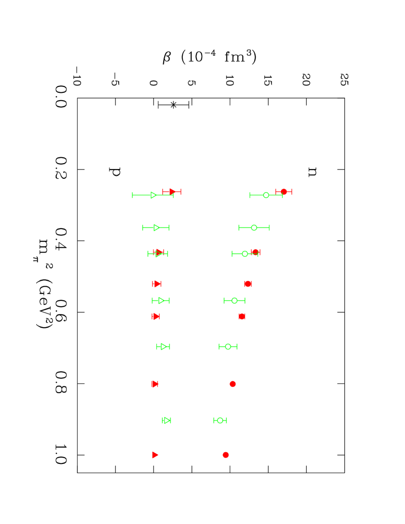
Figure 58: Pion mass dependence of the nucleon magnetic polarizabilities in the quenched approximation (from [LKZW05]).

Figure 59: Pion mass dependence of the neutron electric polarizability in the quenched approximation (from [CWLZ05]). Note that the overall sign of the lattice data should be inverted for comparison with experiment [S⁺07].

Extensive studies of hadron electric and magnetic polarizabilities in quenched lattice QCD have been presented in [CWLZ05] and [LZWC06], respectively. As described in sections 3.7,2.1.10, the electric, $\alpha_{E}$, and magnetic, $\beta_{M}$, polarizabilities lead to hadron mass shifts in the presence of static external electric, $\mathbf{E}$, and magnetic, $\mathbf{B}$, fields, i.e. $\Delta m(E)=m(E)-m(0)=-\alpha_{E}\mathbf{E}^{2}/2$ and $\Delta m(B)=m(B)-m(0)=-\beta_{M}\mathbf{B}^{2}/2$. Here we have already dropped possible contributions that are odd in the external fields, for example a magnetic moment contribution $-\boldsymbol{\mu}\cdot\mathbf{B}$, which are usually removed by considering averages over positive and negative valued fields. In quenched lattice QCD, the static external fields can be implemented by multiplying the link variables that enter the calculation of the quark propagators by phase factors, for example $U_{z}\rightarrow\exp(ie_{q}A_{z})U_{z}$ with a gauge potential $A_{z}(t)=\mathbf{E}_{z}t$ for a static electric field in $z$-direction, or $U_{y}\rightarrow\exp(ie_{q}A_{y})U_{y}$ with a gauge potential $A_{y}(\mathbf{x})=\mathbf{B}_{z}\mathbf{x}_{x}$ for a static magnetic field in $z$-direction. As discussed above in section 3.7, such additional $t$- or $\mathbf{x}$-dependent phase factors are in general in conflict with the (periodic) boundary conditions for the link variables on a finite lattice, and the electromagnetic fields have in principle to fulfill certain quantization conditions.

In [CWLZ05] and [LZWC06], a linearized version of the phase factors, $\exp(iq_{f}A)U\rightarrow(1+iq_{f}A)U$, was used together with Dirichlet boundary conditions in the respective directions. Four different values for the electric and for the magnetic fields were used, that allowed the extraction of the polarizabilities as coefficients of the $E^{2}$- and $B^{2}$-dependences from parabolic fits to the effective mass shifts. The effective mass shifts were obtained in a standard way from the exponential decay of hadron two-point functions in the presence/absence of the external fields. Most of the calculations were based on Wilson fermions and the Wilson gauge action, with pion masses in the range $m_{\pi}\approx 512,\ldots,1000\text{ MeV}$, for a lattice spacing of $a\approx 0.1\text{ fm}$ and a volume of $V\approx(2.4\text{ fm})^{3}$. Results for the for the proton and neutron magnetic polarizabilities as functions of the pion mass are shown in Figure 59, which may be compared to the average values from the PDG of $\beta_{M}^{p}=1.9(5)\cdot 10^{-4}$ for the proton, and of $\beta_{M}^{n}=3.7(2.0)\cdot 10^{-4}\text{ fm}^{3}$ for the neutron [A⁺08i]. While the lattice data points for $\beta_{M}^{p}$ are overall consistent with the value from experiment, the lattice results for the neutron magnetic polarizability are surprisingly different and show a trend towards large values of $\beta_{M}^{n}$ at smaller pion masses. Further calculations for a similar range of pion masses were performed based on clover improved Wilson fermions and a Lüscher-Weisz gauge action, for a lattice spacing of $a\approx 0.17\text{ fm}$ and a volume of $V\approx(2\text{ fm})^{3}$. Corresponding lattice results for the neutron electric polarizability are displayed in Fig. 59 [CWLZ05], which may be compared to the PDG average of $\alpha_{E}^{n}=11.6(1.5)\cdot 10^{-4}\text{ fm}^{3}$ [A⁺08i]. Importantly, it has been noted in [S⁺07] that the real-valued electric field used in [CWLZ05] in the (linearized) lattice phase factor, $U_{z}\rightarrow(1+ie_{q}\mathbf{E}_{z}t)U_{z}$, corresponds to an imaginary electric field in Minkowski space, $\mathbf{E}_{\text{Mink}}=i\mathbf{E}$, so that the sign of the mass shift has to be flipped, $\Delta m(E)=m(E)-m(0)=-\alpha_{E}\mathbf{E}_{\text{Mink}}^{2}/2=\alpha_{E}\mathbf{E}^{2}/2$. Consequently, the signs of the lattice data points in Fig. 59 should be flipped for comparison with the experimental value, turning the consistency of the lattice results with experiment that was observed in [CWLZ05] into a strong disagreement, $\alpha^{n,\exp}_{E}=11.6(1.5)\cdot 10^{-4}\text{ fm}^{3}$ compared to $\alpha^{n,\text{lat}}_{E}\approx-12(4)\cdot 10^{-4}\text{ fm}^{3}$ at the lowest accessible pion mass. These results have been challenged in a number of recent lattice calculations, which may also provide possible explanations for the observed striking discrepancy. Using a full, non-linearized, (real-valued) phase factor, $U_{z}\rightarrow\exp(e_{q}\mathbf{E}_{z}t)U_{z}$, together with periodic boundary conditions, calculations in quenched lattice QCD of the neutron electric polarizability were performed for domain wall as well as clover improved fermions and a renormalization improved gauge action in [S⁺07]. For the domain wall calculation with a lattice spacing of $a\approx 0.1\text{ fm}$ in a volume of $V\approx(1.6\text{ fm})^{3}$, a positive value of $\alpha_{E}^{n}=1.32(2)\cdot 10^{-4}\text{ fm}^{3}$ was found at a large pion mass ($m_{\pi}/m_{\rho}\approx 0.88$). The clover improved Wilson fermion results for the same lattice spacing, but a larger volume of $V\approx(2.4\text{ fm})^{3}$, are shown in Fig. 60 versus the squared pion mass, also providing positive values of the order of $\alpha_{E}^{n}\approx 2.0\cdot 10^{-4}\text{ fm}^{3}$.

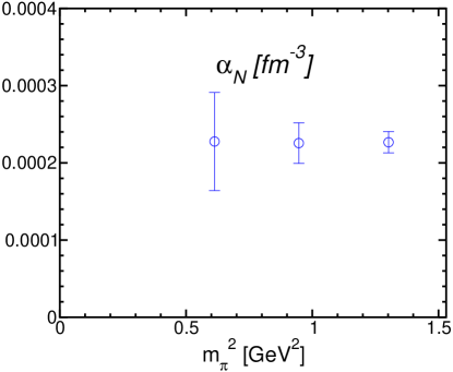
Figure 60: Pion mass dependence of the neutron electric polarizability (from [S⁺07]).

More evidence for a small positive value of $\alpha_{E}^{n}$ at similar pion masses has been found in a first study of the neutron polarizability in unquenched lattice QCD [Eng07b]. At first sight, such a calculation appears prohibitively expensive, since the static background fields would have to be included in the generation of the gauge configurations. The alternative method explored in [Eng07b] is to perturbatively expand the neutron two-point function in the electric background field $E$ to the desired order, $\mathcal{O}(E^{2})$, resulting in a set of space-time integrals of correlators, i.e. four-point functions, which only depend on the original gauge links but include explicit insertions of the external fields. Examples for corresponding connected diagram contributions are shown in Fig. 62, where a cross represents an insertion linear in the background gauge potential $A^{\text{ext}}_{\mu}$, and the encircled cross represents a contact term $\propto A^{\text{ext}}_{\mu}{}^{2}$. The relevant four point functions were computed using a standard sequential method, and contributions from disconnected diagrams were evaluated using stochastic sources with complex $Z(2)$ noise, see section 2.3.3. The neutron mass shift can then be extracted from the $t$-slope of the ratio of the expanded two-point function to the two-point function for vanishing background fields, $R_{2}(t)=G_{(E^{2})}(t)/G_{(E=0)}(t)$, i.e. $\Delta m=-R^{\prime}_{2}(t)$, where $t$ is the source-sink separation in the Euclidean time direction. In extracting $\Delta m$ from $R_{2}(t)$, special care has been taken with respect to additional contributions to the mass shift due to a constant background gauge potential $A^{\text{const}}_{z}=-E_{z}t_{0}$ on a finite lattice, where $t_{0}$ is the time for which the background gauge potential vanishes, $A_{z}=\mathbf{E}_{z}(t-t_{0})$. For the details, we refer to the corresponding discussions in [Eng07b, Eng07a], and just note that the final results in [Eng07b] were obtained by demanding that the mass shift is stationary in $A^{\text{const}}_{z}$ (or $t_{0}$). The numerical computations were based on a hybrid approach of domain wall valence fermions and staggered Asqtad sea quarks using gauge configurations provided by the MILC collaboration, as described in [E⁺06a, H⁺08a], for a lattice spacing of $a\approx 0.124\text{ fm}$ and a volume of $V\approx(2.5\text{ fm})^{3}$. A value of $\alpha^{n}_{E}=2.0(9)\cdot 10^{-4}$ fm³ was finally obtained for a pion mass of $\approx 760\text{ MeV}$. Interestingly, this number is well compatible with the results of the quenched calculation displayed in Fig. 60. The question then arises why the results from [CWLZ05], shown in Fig. 59, are so different in magnitude and sign. Possible explanations are the use of Dirichlet boundary conditions in [CWLZ05], the issue of a constant background gauge potential on a finite lattice [Eng07b, Eng07a], and the linearization of the phase factor employed in [CWLZ05]. The use of Dirichlet boundary conditions has been studied in [S⁺07], and the last two points have been investigated in [Eng07b]. Concerning the latter, it has been observed in particular that a linearization of the phase factor excludes contributions with insertions $\propto(A^{\text{ext}}_{\mu}{})^{2}$ as represented on the right hand side in Fig. 62. These are indeed irrelevant in the naive continuum limit, but in general are required to renormalize propagators with two insertions linear in the background gauge field as shown on the left hand side in Fig. 62. Figure 62 explicitly shows that both types of diagrams give substantial contributions to $R_{2}$, which however cancel to a large extent in the sum. In an attempt to understand the results of [CWLZ05], $\alpha^{n}_{E}$ was calculated again for values of $t_{0}$ (related to the constant background potential $A^{\text{const}}_{z}$) resembling the choices in [CWLZ05], and at the same time dropping the contributions from quadratic insertions $\propto A^{\text{ext}}_{\mu}{}^{2}$ to reproduce the situation of a linearized phase factor. Remarkably, these results turned out to be compatible with the findings in [CWLZ05], i.e. $\alpha^{n}_{E}$ was found to be significantly larger and of opposite (negative) sign, albeit with larger statistical errors [Eng07b].

The issues of real versus imaginary potentials in the phase factors and their linearization have also been studied recently in detail by Alexandru and Lee [AL08]. In the framework of a quenched study, they confirmed what has been discussed above, in particular that the use of a proper Euclidean phase factor gives small positive values for $\alpha^{n}_{E}$, in excellent quantitative agreement with the result from [Eng07b], and only slightly below the values in Fig. 60 from [S⁺07]. Furthermore, it was shown that a linearization of the phase factor leads to large negative values for the polarizability, fully consistent with the earlier results from [CWLZ05] displayed in Fig. 59 (when using the appropriate sign).

In any case, the results for the neutron electric polarizability from quenched lattice QCD in Fig. 60 and from the unquenched calculation discussed above [Eng07b] at pion masses around $600\text{ MeV}$ are approximately a factor of $5$ below the experimental average. This may be expected from ChPT calculations, which predict that $\alpha^{n}_{E}$ diverges as $1/m_{\pi}$ to $+\infty$ in the chiral limit [BKKM92]. Calculations at lower pion masses with better statistical precision have to be performed before a fully quantitative comparison of lattice results with experiment may be attempted using ChPT.

Figure 61: Contributions to the neutron two-point function expanded in the external gauge potential to $\mathcal{O}(A_{\mu}^{2})$ (from [Eng07b]).

Figure 62: Contributions of diagrams as in Fig. 62 to the ratio $R_{2}(t)$ (from [Eng07b]).

The electric polarizabilities of neutral and charged hadrons have very recently also been studied in unquenched lattice QCD in a mixed action approach based on the $n_{f}=2+1$ domain wall configuration from the RBC-UKQCD collaboration and tadpole-improved Clover-Wilson fermions for the valence quarks [DTWL08]. In contrast to the unquenched study in [Eng07b] discussed above, the calculation was mainly based on the energy shifts extracted directly from the corresponding hadron two-point functions. Effects from a coupling of the sea quarks to the electric background field were not included (“$U(1)$-quenched” [LMW08]). As usual, the electric field was implemented by multiplying the gauge links by $U(1)$ links of the form $U^{\text{EM},\text{ext}}_{\mu=z}=\exp(-ie_{q}E_{\text{\text{EM}}}t)$ with real valued $E_{\text{EM}}$ (requiring an analytic continuation to Minkowski space). Particular attention has been paid to the quantization conditions on a periodic lattice (see our discussion in section 3.7). It was argued that by including additional transverse links at the time boundary, the electromagnetic flux represented by the plaquette can be rendered continuous across the boundary if the electric field obeys the relaxed quantization condition $qE=2\pi n/(L_{t}L_{s})$ with integer $n$ and temporal and spatial lattice extents $L_{t}$ and $L_{s}$, respectively. Comparing effective masses in the presence of constant external electric fields, calculated with and without the transverse link, and with integer and non-integer $n$, the effectiveness of the method was also impressively verified on the numerical side. Values for the electric polarizabilities of different charge-neutral hadrons were obtained from fits to the particle energies as functions of the external field, corresponding to $n=1,-2,3,4,5,-6,7$. A preliminary value of $\alpha^{n}_{E}=3.6(1.3)\cdot 10^{-4}\text{ fm}^{3}$ was obtained for, e.g., the neutron electric polarizability at a pion mass of $m_{\pi}\approx 420\text{ MeV}$, which is in good agreement with the results from [S⁺07, Eng07b] discussed above. Concerning charged particles, it is clear that they will be accelerated in the presence of external electric fields, and at first sight it is not obvious how the two-point functions precisely depend on the Euclidean time, the particle momentum and the constant background field in this case. This has been studied in the non-relativistic limit in an effective field theory framework for a spin-$1/2$ particle coupled to a classical gauge field [DTWL06], where it was found that the exponential fall-off gets modified for charged particles: $C^{h}_{\text{2pt}}(t)\stackrel{{\scriptstyle NR}}{{\rightarrow}}\exp(-E_{h}t-q^{2}E^{2}_{\text{EM}}t^{3}/(6m_{h}))$, where $E_{h}$ is the hadron energy depending on the background field $E_{\text{EM}}$, and where the hadron mass is given by $m_{h}=E_{h}(E_{\text{EM}}=0)$. The energies $E_{h}$ of the charged hadrons in the presence of external fields were extracted from fits to the respective two-point functions using the full functional form of the $t$-dependence of $C^{h}_{\text{2pt}}(t)$. Finally, the electric polarizabilities $\alpha^{h}_{E}$ were obtained from fits to the $E_{\text{EM}}$-dependence of $E_{h}(E_{\text{EM}})=\alpha^{h}_{E}E^{2}_{\text{EM}}/2+\mathcal{O}(E^{4}_{\text{EM}})$. Examples for some of the preliminary results given in [DTWL08] are $\alpha^{\pi^{+}}_{E}=3.4(0.4)\cdot 10^{-4}\text{ fm}^{3}$ the pion, and $\alpha^{p}_{E}=8.8(5.9)\cdot 10^{-4}\text{ fm}^{3}$ for the proton, for $m_{\pi}\approx 420\text{ MeV}$. It would be highly interesting to extend and improve this promising study with respect to the statistics and systematics, for example by investigating potential finite volume and discretization effects, and in particular the pion mass dependence of the results in greater detail.

3.8 Discussion and summary

We have seen substantial progress in hadron form factor calculations in recent years, in particular related to dynamical $n_{f}=2$ and $n_{f}=2+1$ lattice QCD simulations. An overview of results from different collaborations for the pion and nucleon form factors is given in Fig. 63 and 64 for pion charge radius, in Figs. 65 and 66 for the nucleon isovector Dirac and Pauli mean square radii, and in Fig. 67 for the isovector anomalous magnetic moment. It is remarkable that calculations are carried out routinely with pion masses as low as $300\text{ MeV}$ with excellent statistical precision for the pion form factor and in some cases very good precision for the nucleon form factors. The statistics are in general lower for quantities like magnetic moments that have to be extracted from extrapolations of form factors to $Q^{2}=0$.

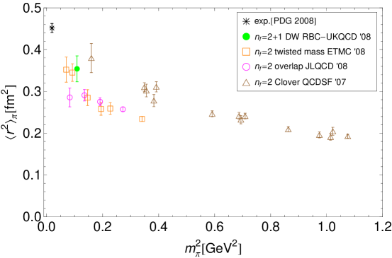
Figure 63: Overview of dynamical lattice QCD results for the pion mean square radius as a function of $m_{\pi}^{2}$.

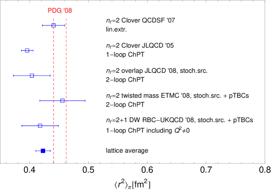
Figure 64: Overview of dynamical lattice QCD results for the chirally extrapolated pion mean square radius at the physical pion mass.

Thanks to the use of advanced methods involving all-to-all propagators, the one-end-trick and partially twisted boundary conditions, great progress has been reported by several collaborations with respect to the pion form factor, where high precision results have been obtained in unquenched lattice QCD for pion masses below $300\text{ MeV}$ and very small, non-zero values of the momentum transfer down to $Q^{2}\approx 0.01\text{ GeV}^{2}$. An overview of corresponding results for the mean square pion charge radius as a function of $m_{\pi}^{2}$ is displayed in Fig. 63. While an overall good consistency can be observed for most of the data points in the range of $m_{\pi}^{2}\approx 0.1,\ldots,0.4\text{ GeV}^{2}$, we note, however, that the data points from the $n_{f}=2$ clover improved Wilson fermion study by QCDSF/UKQCD lie significantly above the rest. This discrepancy may be at least partially due to the different ways $\langle r_{\pi}^{2}\rangle$ has been extracted from the $Q^{2}$-dependence of the form factor data: QCDSF/UKQCD fitted a monopole ansatz with the monopole mass as free parameter to lattice form factor data in a wide range of $Q^{2}=0,\ldots,\approx 4\text{ GeV}^{2}$. The RBC-UKQCD data point was obtained using 1-loop ChPT to describe simultaneously the $m_{\pi}$- and $Q^{2}$-dependence of $F_{\pi}(Q^{2})$ (calculated with pTBCs). JLQCD employed an ansatz based on the $\rho$-meson pole with polynomial corrections, while ETMC also used a monopole ansatz to fit the form factor data in a smaller range of $Q^{2}=0,\ldots,\approx 1.25\text{ GeV}^{2}$ (employing pTBCs). In addition, finite volume effects (although they have been included in several cases), discretization effects, and the setting of the scale may help to explain the observed differences.

The lattice results for the pion charge radius at the physical pion mass presented in Fig. 64 mostly agree within errors, which is remarkable by itself since the chiral extrapolations differ significantly in the details. Most of the central values, as well as the lattice average, are $\approx 10\%$ below the experimental result. It will be an interesting task to work out the precise origin of this discrepancy in future studies of the pion form factor.

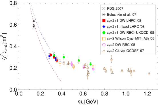
Figure 65: Overview of dynamical lattice QCD results for the isovector Dirac mean square radius. The dashed curve represents the leading 1-loop HBChPT prediction [BKKM92], and the dotted-dashed curve the result obtained in the SSE [G⁺05e], Eq. (134).

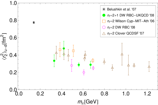
Figure 66: Overview of dynamical lattice QCD results for the isovector Pauli mean square radius.

Moving on to the nucleon form factors, we note that although there is some scatter visible in the case of the Dirac mean square radius in Fig. 65, a general trend towards the experimental value at small pion masses can still be observed. Chiral perturbation theory indeed predicts a steep rise of $\langle r_{1}^{2}\rangle$ towards the chiral limit as indicated by the dashed and dotted-dashed curves, but it seems that for a fully quantitative extrapolation to the physical pion mass, more precise lattice data is needed at pion masses below $300\text{ MeV}$. The statistical uncertainty of the lattice results for $\langle r_{2}^{2}\rangle$ and the anomalous magnetic moment in Figs. 66 and 67, respectively, is $\mathcal{O}(10\%)$ at the lowest pion masses, which must be significantly reduced before a quantitatively meaningful chiral extrapolation and comparison with the very precise experimental values can be performed. Partially twisted boundary conditions could help in these cases as they promise access to very small, non-zero values of the momentum transfer, and thereby significantly reduce the errors induced by the extrapolations based on, e.g., dipole fits to $Q^{2}=0$. For the presently accessible pion masses and statistics, a clear, systematic difference between the $n_{f}=2$ and $n_{f}=2+1$ cannot be observed for any of these observables.

Discrepancies between lattice data points that are observed even when statistical uncertainties are taken into account indicate the presence of systematic effects. Interestingly, in several cases finite volume and also discretization effects have been checked at least semi-quantitatively and were found to be smaller than the statistical errors. It may, however, be deceptive to assume that systematic errors are completely negligible in such cases. It would be very helpful if at least rough quantitative estimates of systematic uncertainties, including errors due to the setting of the lattice scale in physical units, would be routinely provided. From the overview plots in Figs. 65, 66 and 67, and the comparisons with the experimental data points it is in any case clear that a strong pion mass dependence is expected in the region below $\approx 300\text{ MeV}$. Obviously, while there is at least qualitative agreement with results from ChPT, naive linear extrapolations in $m^{2}_{\pi}$ from the currently accessible pion masses to the physical pion mass fail in general and should be avoided.

To this date, most lattice results for nucleon form factors are given in the isovector channel, where contributions from quark line disconnected diagrams drop out because of isospin symmetry. Estimates of disconnected contributions, even if only in the form of upper limits, would be very useful and allow to provide first quantitative results for the equally important isosinglet sector and the contributions from individual flavors.

An overview of lattice results for the nucleon axial vector coupling constant as a function of $m_{\pi}$ and the spatial box size $L$ is given in Fig. 68. The required renormalization of the axial vector current has been carried out in all cases non-perturbatively, where simulations with domain wall fermions have the clear advantage that $g_{A}/g_{V}$ is automatically renormalized due to the lattice chiral symmetry. Although the $g_{A}$-landscape in $m_{\pi}^{2}$ and box length $L$ is not completely smooth, in particular due to the low lying data points from RBC-UKQCD at low pion masses, it clearly shows that $g_{A}$ tends towards lower values as the box length decreases. In this case, finite volume effects are no longer necessarily seen as systematic uncertainty: The volume dependence has been included and studied in the framework of ChPT [BS04, K⁺06], and as no new low energy constants have to be introduced at finite volume, the $L$-dependence of $g_{A}$ provides an additional handle in the matching of ChPT predictions and lattice results. A fit to the simultaneous $m_{\pi}$- and $L$-dependence of the lattice data for $g_{A}$ based on ChPT may therefore help to better constrain the universal low energy constants and provide a more accurate and precise chiral and infinite volume extrapolation. This has already been attempted quite successfully in [K⁺06], however the application of results from ChPT to the rather large pion masses of $m_{\pi}\gtrapprox 600\text{ MeV}$ accessible in this work should be regarded with some caution.

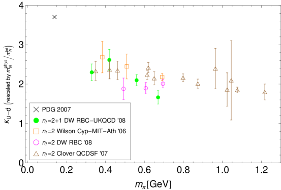
Figure 67: Overview of dynamical lattice QCD results for the isovector anomalous magnetic moment.

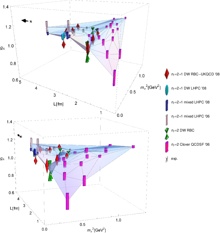
Figure 68: The “$g_{A}$-landscape”, giving an overview of dynamical lattice QCD results for the nucleon isovector axial vector coupling constant.

In addition to the Dirac and Pauli form factors and the axial vector coupling of the nucleon, a broad range of interesting observables like tensor form factors of the pion and the nucleon, and electromagnetic form factors of the $\rho$-meson and the $\Delta$-baryon have by now been studied in dynamical lattice QCD. Many of these quantities are very difficult to access in experiment, and lattice calculations therefore often provide at least qualitatively important insights into the charge distributions, magnetization densities, possible deformations and the spin structure of hadrons.

An example of an observable that can be accessed in lattice QCD with a precision similar to $g_{A}$, but is difficult to determine directly in experiment, is the tensor charge $g_{T}$ of the nucleon. An overview of non-perturbatively renormalized lattice results for $g^{u-d}_{T}$ in the $\overline{\text{MS}}$ scheme at a scale of $4\text{ GeV}^{2}$ is given in Fig. 69. The lattice data points, which show a remarkable statistical precision, may be compared to results for the valence quark contribution to $g^{u-d}_{T}$ obtained from a phenomenological description of SIDIS data [A⁺08j] as indicated by the star.

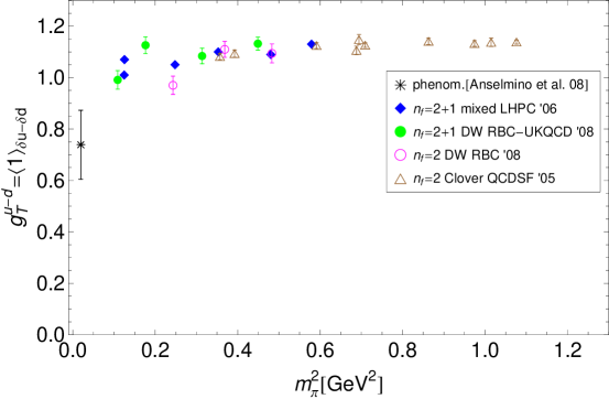
Figure 69: Overview of dynamical lattice QCD results for the nucleon isovector tensor charge $g^{u-d}_{T}=A^{u-d}_{T10}(t\text{{=}}0)$, see Eq. (22).

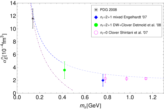
Figure 70: Overview of lattice QCD results for the electric polarizability of the neutron $\alpha^{n}_{E}$. Predictions from 1-loop HBChPT [BKM95] and SSE [HGHP04] are represented by the dashed and dot-dashed curves, respectively, which have been continued to larger pion masses only to guide the eye.

In particular with the help of improved background field methods, very interesting studies have been performed of the magnetic moment of the $\Delta$-baryon and nucleon polarizabilities.

Concerning the electric polarizability of the neutron, there is mounting evidence from different lattice studies that $\alpha^{n}_{E}\approx 2\ldots 3\cdot 10^{-4}\text{ fm}^{3}$ for pion masses $m_{\pi}\gtrapprox 400\text{ MeV}$, as shown in the overview plot Fig. 70. In view of the different techniques that were used for the extraction of the polarizabilities (though all were based on the background field method), it is gratifying to see that the results not only agree in sign but also in magnitude within errors. As we have noted before, comparatively low values at unphysically large pion masses were to be expected from ChPT, predicting that $\alpha^{n}_{E}$ diverges as $1/m_{\pi}\rightarrow+\infty$ in the chiral limit. This is adequately illustrated by the dashed curve in Fig. 70, representing a 1-loop HBChPT calculation [BKM95]. It would be very interesting to improve the statistics of the lattice calculations, extend them to lower pion masses and investigate if a quantitatively reliable chiral extrapolation to the physical pion can be performed.

4 Lattice results on parton distribution functions and generalized parton distributions

4.1 Overview of lattice results

4.1.1 Pion

First calculations of the lowest two moments of the pion quark distribution function, $\langle x\rangle^{\pi}$ and $\langle x^{2}\rangle^{\pi}$, in quenched lattice QCD have been presented in the pioneering works by Martinelli and Sachrajda in the late 1980’s [MS87b, MS88]. An extensive study in the quenched approximation, including the next higher moment $\langle x^{3}\rangle^{\pi}$, was presented many years later in [B⁺97]. The ZeRo collaboration has studied the momentum fraction of quarks in the pion in some detail in quenched QCD, employing non-perturbative renormalization of the corresponding operators and including an investigation of finite size effects [G⁺03, G⁺04b, G⁺05h]. A detailed study of $\langle x\rangle^{\pi}$ using twisted mass fermions in the quenched approximation has been presented by the $\chi$LF collaboration [C⁺06a]. Preliminary (unrenormalized) results for the momentum fraction of quarks in the pion in unquenched lattice QCD, based on twisted mass fermions, were obtained by the European Twisted Mass collaboration [B⁺07b]. A detailed study of the lowest moments, $\langle x^{n-1}\rangle^{\pi}$ with $n=2,\ldots,4$, of the pion PDF in unquenched lattice QCD has been presented by QCDSF [B⁺07h]. First results for moments of the pion vector GPD, in particular for the generalized form factor (GFF) $A^{\pi}_{20}(t=q^{2})$ in Eq. (10), in unquenched lattice QCD were presented earlier by QCDSF in [B⁺06e], and a calculation of the lowest moments moments of the pion tensor GPD in the same simulation framework was published recently [B⁺08h]. The momentum fraction carried by gluons in the pion has been investigated for the first time in [MN08] in the quenched approximation.

4.1.2 Nucleon

The lowest two moments of the unpolarized nucleon PDF were calculated already twenty years ago in the quenched approximation [MS89]. Thereafter, moments of unpolarized and polarized nucleon PDFs have been investigated in quenched lattice QCD in a number of works by Göckeler et al. [G⁺96b, G⁺97a, G⁺01]. A first detailed study of moments of unpolarized, polarized and tensor (transversity) PDFs in unquenched and quenched lattice QCD by LHPC/SESAM can be found in [D⁺02]. Preliminary results for the unpolarized quark momentum fraction in quenched lattice QCD using overlap fermions were presented in [G⁺05i], and a quenched calculation of moments of unpolarized and polarized PDFs employing domain wall fermions is described in [OBO06]. A careful investigation of the unpolarized momentum fraction, $\langle x\rangle$, of quarks in the nucleon in the quenched approximation, using an improved action and employing non-perturbative renormalization, was presented by QCDSF [GHP⁺05]. The quark momentum fraction has also been studied by LPHC in the framework of a lattice investigation of GPDs with dynamical quarks in [H⁺08a], where also numerical results for the higher moment, $\langle x^{2}\rangle$, and the moments of the polarized PDFs can be found. Recently, the isovector polarized and unpolarized quark momentum fractions have been computed by RBC and UKQCD in unquenched lattice QCD using domain wall fermions [LBO⁺08, OY08]. A number of more recent results on moments of quark PDFs obtained in dynamical lattice QCD appeared in proceedings, see, e.g., [E⁺06b, R⁺07, G⁺07f, B⁺07g]. An attempt to extract the unpolarized PDF as a function of the momentum fraction $x$ from lattice results for the lowest $x$-moments has been presented in [DMT01].

Angular momentum contributions to the nucleon spin have been first investigated in quenched lattice QCD in [MDL⁺00] and, based on a different method avoiding extrapolations in the momentum transfer, in [GJJ02], where in both cases also contributions from disconnected diagrams have been evaluated. First studies of moments of unpolarized nucleon generalized parton distributions, i.e. the generalized form factors $A_{20}(t=q^{2})$, $B_{20}(t)$ and $C_{20}(t)$ in Eq. (27), appeared in 2003 in the quenched approximation by QCDSF [G⁺04a] and in unquenched lattice QCD by LHPC/SESAM[H⁺03]. Higher moments of GPDs were investigated in unquenched lattice QCD in [H⁺04]. More recently, an extensive study of the polarized and unpolarized moments of GPDs with dynamical quarks in a mixed action approach has been presented by LHPC [H⁺08a]. Nucleon tensor (generalized) form factors $g_{T}(t)=A_{T10}(t)$ and $A_{T20}(t)$ in Eqs. (22) and (29), including the $x$-moment of the transversity distribution $\langle x\rangle_{\delta}=A_{T20}(t\text{{=}}0)$, have been calculated in unquenched lattice QCD by QCDSF [G⁺05g]. The transverse spin structure of the nucleon, including in particular the tensor (generalized) form factors $\overline{B}_{T10}=B_{T10}+2\widetilde{A}_{T10}$ in Eq. (22), was studied in the same simulation framework by QCDSF in [G⁺07d]. As before, a number of results on moments of GPDs in unquenched lattice QCD can be found in proceedings, see, e.g., [G⁺05c, G⁺06a, G⁺05b, G⁺07c, B⁺07g, S⁺04, N⁺04, E⁺06b, B⁺08f].

Turning to the gluon structure of the nucleon, we note that the first and only attempt to extract the gluon contribution to the nucleon spin, $\Delta g$, in quenched lattice QCD has been made almost 20 years ago in [Man90] (see also the pertinent comments in [EST91] and a reply in [Man91]). The unpolarized gluon momentum fraction in the nucleon has been investigated so far only in [G⁺97b] more than 10 years ago in the quenched approximation.

4.1.3 $\rho$-meson

The only lattice QCD calculation of moments of unpolarized and polarized PDFs of the $\rho$-meson in the quenched approximation was published more than ten years ago in [B⁺97]. So far, there are no lattice results available for moments of GPDs of the $\rho$-meson, apart from the lowest $n=1$-moments corresponding to the $\rho$-meson electromagnetic FFs discussed above in section 3.5.

4.2 Results from chiral perturbation theory

Moments of unpolarized PDFs have been studied at leading 1-loop level in ChPT for the pion and the nucleon (in HBChPT) by Arndt and Savage in [AS02], where also contributions from explicit $\Delta$-DOFs were included. Leading non-analytic corrections for the complete set of twist-2 nucleon matrix elements, i.e. the moments of the unpolarized, polarized and transversity PDFs, were independently obtained in HBChPT by Chen and Ji [CJ01]. The inclusion of $\Delta(1232)$-degrees of freedom ($\Delta$-DOFs) was also studied in [DMT02] for moments of the isovector twist-2 PDFs of the nucleon. A partially-quenched ChPT study of isovector twist-2 matrix elements of baryons including $\Delta$-DOFs can be found in [CS02, BS02]. More recently, finite volume corrections to twist-2 nucleon matrix elements were investigated in some detail in [DL05] to leading 1-loop order in partially-quenched HBChPT. Leading chiral corrections to the angular momentum contributions of quarks and gluons to the proton spin, $J_{q,g}$ have been calculated in [CJ02], in the framework of HBChPT including $\Delta$ intermediate states. Subsequently, the pion mass and momentum dependence of form factors of the energy momentum tensor, i.e. the gravitational form factors, for the nucleon in the isovector and isosinglet channel has been worked out to leading 1-loop order in HBChPT [BJ02]. The complete set of moments of the nucleon vector, axial-vector and tensor GPDs has been investigated in [ACK06] in HBChPT to leading 1-loop order. Moments of the unpolarized and polarized (vector and axial-vector) nucleon GPDs in the isosinglet channel were also calculated in [DMS06] to leading 1-loop order in HBChPT. Corresponding results in ChPT including the isovector case and moments of tensor GPDs of the pion and the nucleon were presented by the same authors in [DMS07]. A calculation of the isovector and isosinglet gravitational form factors of the nucleon, including a study of the quark angular momentum contribution to the nucleon spin, was also recently performed in covariant BChPT to $\mathcal{O}(p^{2})$ based on a modified infrared regularization scheme [DGH08]. Leading non-analytic chiral corrections to the moments of the pion vector GPDs were already studied in [KP02] and later revisited in [DMS05]. More recently, finite volume corrections to pion matrix elements of vector and tensor operators were calculated in [MS07].

4.3 Moments of PDFs

In this section, we are mainly concerned with the lowest $x^{n-1}$-moments of the quark PDFs of the pion, nucleon and $\rho$-meson, see Eqs. (54,55,56) and adjacent discussion, which can be directly obtained from corresponding forward hadron matrix elements of the local operators in Eq. (3).

4.3.1 Pion

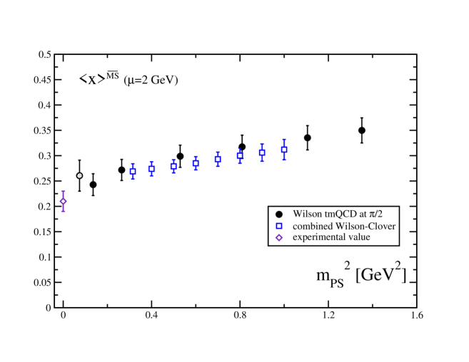
Figure 71: The momentum fraction of up-quarks in a $\pi^{+}$ (from [C⁺06a]).

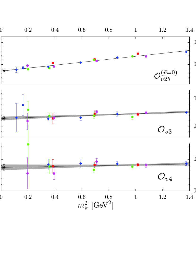
Figure 72: The momentum fraction of up-quarks in a $\pi^{+}$ (from proceedings [B⁺07h]).

The $\chi_{\text{L}}\text{F}$ collaboration has calculated the momentum fraction of quarks in the pion, $\langle x\rangle^{\pi}$, in the quenched approximation using Wilson twisted mass fermions and the standard Wilson gauge action for a wide range of pion masses from $\approx 270\text{ MeV}$ to $\approx 1160\text{ MeV}$, for up to five different lattice spacings from $\approx 0.123\text{ fm}$ down to $\approx 0.048\text{ fm}$ and volumes in the range of $\approx(1.5,\ldots,2.0\text{ fm})^{3}$ [C⁺06a]. Employing the Schrödinger functional renormalization scheme, the underlying twist-2 operator

$$\mathcal{O}^{n=2}_{v}=(\mathcal{O}_{44}-1/3(\mathcal{O}_{11}+\mathcal{O}_{22}+\mathcal{O}_{33}))\,,$$ (144)

a linear combination of the operators listed in Eq. (116), has been non-perturbatively renormalized, and the results have been transformed to the $\overline{\text{MS}}$-scheme at a scale of $\mu=2\text{ GeV}$. Finite volume effects, which are non-negligible for some of the accessed pion masses and lattice volumes, have been taken into account following the study in [G⁺04b], where good agreement between a power-law, $\propto 1/L^{p}$, and an exponential, $\propto\exp(cL)$, ansatz for the volume dependence (with constants $p,c$) was found. Results for different lattice spacings were utilized in a careful study of the continuum limit, exhibiting sizeable $\mathcal{O}(a^{2})$ discretization effects at low pion masses in the case where the vanishing of the pion mass was used for the definition of the critical quark mass $m_{c}$ (critical hopping parameter $\kappa_{c}$), and much smaller scaling violations for the PCAC definition of $m_{c}$. A linear extrapolation in $a^{2}$ to the continuum limit was performed, and the corresponding results for $\langle x\rangle^{u}_{\pi}$ as a function of $m_{\pi}^{2}$, including finite volume corrections, are shown in Fig. 72 as filled circles. The lattice data point at the lowest pion mass of $\approx 270\text{ MeV}$, denoted by the shaded circle, was not extrapolated to the infinite volume limit. Apart from the lattice data point at $m_{\pi}\approx 370\text{ MeV}$, the results appear, to a good approximation, to be linear in $m_{\pi}^{2}$.

Although a direct quantitative comparison with results from experiment and phenomenology is not possible due to the nature of the quenched approximation, we note that the central values of the lattice data points at the lowest accessible pion masses lie approximately 15% above the value of $\langle x\rangle^{u,v}_{\pi}=0.217(11)$ obtained for the valence quark sector (not including possible contributions from anti-quarks) in a recent phenomenological analysis of Drell-Yan scattering data [WRH05]. It is reassuring that the lattice data points of the twisted mass approach agree well within errors with the results of a comparable lattice study by the ZeRo collaboration based on clover-improved Wilson fermions [G⁺03, G⁺04b, G⁺05h], denoted by the open squares in Fig. 72.

We now turn to a discussion of results from QCDSF obtained in the framework of lattice simulations with $n_{f}=2$ flavors of clover-improved Wilson quarks and the Wilson gauge action [B⁺07h]. Calculations have been performed for pion masses ranging from $\approx 350\text{ MeV}$ to $\approx 1200\text{ MeV}$, lattice spacings of $a\approx 0.07,\ldots,0.12\text{ fm}$, and volumes of $\approx(1.3,\ldots,2.5\text{ fm})^{3}$, including dedicated finite volume runs. Local lattice operators with one, two and three covariant derivatives, needed for the computation of the $x^{n-1}$-moments $\langle x\rangle_{\pi}$, $\langle x^{2}\rangle_{\pi}$ and $\langle x^{3}\rangle_{\pi}$, have been non-perturbatively renormalized using the Rome-Southampton method, and the results were given in the $\overline{\text{MS}}$ scheme at a scale of $\mu=2\text{ GeV}$. While the extraction of $\langle x\rangle^{\pi}$ based on the operator in Eq. 144 can be done for zero pion momentum, $\mathbf{P}=0$, a non-zero $\mathbf{P}$ is require to obtain non-vanishing pion matrix matrix elements for the higher moments based on the operators

$$\mathcal{O}^{n=3}_{v} = \mathcal{O}_{144}-1/2(\mathcal{O}_{224}+\mathcal{O}_{334})\,,$$ (145)

$$\mathcal{O}^{n=4}_{v} = \mathcal{O}_{1122}+\mathcal{O}_{1133}+\mathcal{O}_{2244}+\mathcal{O}_{3344}-2\left(\mathcal{O}_{1144}+\mathcal{O}_{2233}\right)\,.$$ (146)

Consequently, the higher moments are subject to larger statistical noise. Figure 72 displays the corresponding lattice results for $\langle x^{n-1}\rangle^{u}_{\pi^{+}}$ with $n=2,\ldots,4$ versus $m_{\pi}^{2}$, together with linear chiral extrapolations represented by the shaded bands. A study of the volume dependence showed that finite size effects may be of the order of a few percent already for $m_{\pi}L\approx 5$ and up to 10% for the lowest pion masses included in Fig. 72. For comparison, see also the results in [G⁺04b]. Finite volume effects (FVEs) are therefore significant with respect to the statistical errors for $\langle x\rangle_{\pi}$. In an attempt to correct for FVEs, an ansatz

$$\langle x^{n-1}\rangle^{u}_{\pi^{+}}=c_{n,0}+c_{n,1}m_{\pi}^{2}+c_{n,2}m_{\pi}^{2}e^{-m_{\pi}L}\,,$$ (147)

including a term with an exponential dependence on the lattice extent $L$, was used to fit the lattice data points. A value of $\langle x\rangle^{u}_{\pi^{+}}=0.271\pm 0.002_{(\text{stat})}\pm 0.010_{(\text{ren})}$ was obtained for the momentum fraction of up-quarks in the $\pi^{+}$ at the physical point and in the infinite volume, where the second error represents uncertainties from the non-perturbative renormalization. For a comparison of the $(n=2,\ldots,4)$-moments in Fig. 72 with quenched lattice calculations and results from phenomenological studies of the pion PDFs in [SMRS92, GRS99], we refer to [B⁺07h]. We note, however, that such a direct comparison has to be considered with caution, since a number of different approximations and assumptions have been employed in either of these studies. In particular, contributions from disconnected diagrams, which are present for even $n$, have not been included in the lattice calculations.

Recently, Negele and Meyer performed a first calculation of the momentum fraction carried by gluons in the pion, $\langle x\rangle^{\pi}_{g}$, using the Wilson action in the quenched approximation [MN08]. Noting that $\langle\pi|\bar{T}^{g}_{00}|\pi\rangle=N\langle x\rangle^{\pi}_{g}$, where $N$ is a kinematic factor and $\bar{T}^{g}_{\mu\nu}$ is the traceless part of the gluon energy momentum tensor, the numerical studies were based on plaquette and clover discretizations of the operator $\bar{T}^{g}_{00}=(-\mathbf{E}^{2}+\mathbf{B}^{2})/2$, where, e.g., $\mathbf{E}^{2}=\sum_{a}\mathbf{E}^{a}\cdot\mathbf{E}^{a}$. HYP-smearing of the gauge fields was employed to reduce the statistical noise of the correlators due to short-range fluctuations of the gauge fields, which represents a major challenge in calculations of gluonic contributions to hadron structure observables. To preserve locality as much as possible, the plaquette operator was used together with HYP-smearing for the final calculations, providing a reduction of the variance by a factor of $\approx 40$ compared to the unsmeared case. The gluon operator, which mixes with the quark singlet operator $\bar{T}^{q}_{00}$ under renormalization, was (partially) non-perturbatively renormalized, employing results from [G⁺03, G⁺05h] for the quark non-singlet renormalization constant and the bare quark momentum fraction. Computations were performed for three different pion masses from $\approx 620\text{ MeV}$ to $\approx 1060\text{ MeV}$, giving a value of $\langle x\rangle^{\pi}_{g}=0.37\pm 0.08_{(\text{stat})}\pm 0.12_{(\text{ren})}$ in the $\overline{\text{MS}}$ scheme at a scale of $\mu=2\text{ GeV}$, for a pion mass of $m_{\pi}\approx 890\text{ MeV}$. Since the value of one of the renormalization constants was not known beyond its trivial tree-level value, a systematic error of $\pm 0.12$ was added to account for higher order contributions. The result indicates that even for such large pion masses, the gluons carry a substantial fraction of the total momentum of the parent hadron. It would be highly interesting to repeat this study in full QCD and to reduce in particular the systematic uncertainties due to the operator renormalization.

4.3.2 Nucleon

In the following, we will be concentrating on the isovector case, for which only contributions from connected diagrams are relevant. The computationally much more demanding disconnected contributions are, to this date, not routinely included in lattice hadron structure calculations. Still, a large number of interesting results have been obtained over the years for the connected parts of isosinglet quark contributions to observables. Some of those will be discussed in particular in relation with the spin structure of the nucleon below in section 4.4.3.

Unpolarized quark momentum fraction

Already the pioneering work by Martinelli and Sachrajda in the late 1980’s indicated that the isovector momentum fraction of quarks in the nucleon, as obtained from lattice QCD simulations in the quenched approximation, is approximately $\approx 50\%$ larger than the result from experiment and phenomenology, i.e. $\langle x\rangle_{u-d}^{\text{lat}}\approx 0.25$ compared to $\langle x\rangle_{u-d}^{\text{pheno}}\approx 0.16$ (in the $\overline{\text{MS}}$ scheme at a scale of $\mu=2\text{ GeV}$). Recent global PDF-analyses of DIS, Drell-Yan, and other scattering data give, e.g., $\langle x\rangle_{u-d}^{\text{CTEQ6.6}}\simeq 0.154$ [N⁺08a] and $\langle x\rangle_{u-d}^{\text{MRST06}}\simeq 0.158$ [MSTW07], see also [MRST03, MRST04, AMP06].

Years later, the initial quenched lattice results were confirmed with higher precision and for pion masses down to $\mathcal{O}(600\text{ MeV})$ in [G⁺96b]. Since then, a number of possible explanations and solutions for the discrepancy have been suggested, as summarized by the following keywords:

• quenched approximation

• renormalization of the underlying lattice operators

• discretization effects

• finite volume effects

• phenomenological analysis of experimental data giving $\langle x\rangle^{u-d}_{\text{exp}}$

• chiral extrapolation

A first extensive study based on simulations with $n_{f}=2$ dynamical Wilson fermions by the LHPC-SESAM collaboration [D⁺02] confirmed again the earlier findings in the quenched approximation at similar pion masses. Several years later, many of the above items were looked at in great detail in the framework of a quenched lattice QCD study using clover-improved Wilson fermions [GHP⁺05]. First, a reanalysis of moments of structure functions, which in contrast to the PDFs are directly accessible in experiment, revealed good agreement with the results obtained from global PDF-analyses. On the side of the lattice calculation, operator improvement terms were studied and found to be numerically small, and different perturbative and non-perturbative renormalization procedures were investigated and compared, including the possibility of operator mixing. Non-perturbatively renormalized operators were then used to obtain the final results for the momentum fraction, which were found to be practically independent of the pion mass in the accessible range of $m_{\pi}\approx 550$ to $m_{\pi}\approx 1250\text{ MeV}$. Separate linear extrapolations in $m^{2}_{\pi}$ to the chiral limit were performed for three different values of the lattice spacing, and these values were finally extrapolated linearly in $a^{2}$ to the continuum limit. All these efforts culminated in a value of $\langle x\rangle^{u-d}_{\text{lat}}=0.245(9)$ in the $\overline{\text{MS}}$ scheme at a scale of $2\text{ GeV}$ [GHP⁺05], in perfect agreement with the results obtained in the years before in quenched and unquenched lattice QCD, where only perturbatively renormalized operators have been employed. Although new discrepancies within different lattice approaches emerged more recently, as will be discussed below, it is likely that a proper, non-linear, chiral extrapolation of $\langle x\rangle^{u-d}$ to the physical pion mass is the clue for bridging at least part of the large gap of $\approx 50\%$ between the lattice results and the experimentally observed value. Some of the attempts to reach agreement at the physical point based on various forms of chiral extrapolations will be discussed in the following. Results for the quark momentum fractions obtained in the framework of lattice studies of moments of GPDs will be discussed in some detail in section 4.4.2 further below.

Figure 73: The momentum fraction of quarks in the isovector channel, $\text{v}_{2}^{u-d}=\langle x\rangle^{u-d}$ (from proceedings [G⁺07c]).

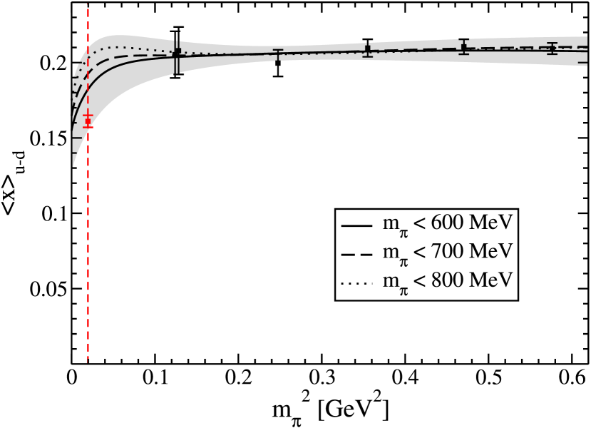
Figure 74: The isovector momentum fraction of quarks (from proceedings [R⁺07]).

The situation just described is reflected in the more recent results for $\langle x\rangle^{u-d}$ from QCDSF displayed in Fig. 74 as a function of the pion mass [G⁺07c], for $n_{f}=2$ flavors of clover-improved Wilson quarks and the Wilson gauge action. The lattice data points, which have been obtained using the non-perturbatively renormalized lattice operator $\mathcal{O}_{v2b}=\mathcal{O}^{n=2}_{v}$ in Eq. 144, are not only practically flat in $m_{\pi}^{2}$ over the full range of $m_{\pi}\approx 350,\ldots,1400\text{ MeV}$, they also agree within statistics for all the different ensembles with lattice spacings of $a\approx 0.07,\ldots,0.12\text{ fm}$ and volumes of $\approx(1.3,\ldots,2.5\text{ fm})^{3}$, with $m_{\pi}L\gtrsim 3.5$. In particular, there are no significant discretization effects visible, which was already observed for a similar set of ensembles in [G⁺05a] and more recently confirmed in [B⁺08i]. Finite size effects have been analyzed in a similar lattice framework for a pion mass of $\approx 770\text{ MeV}$ and were found to be small compared to the statistical errors [G⁺05a], although they have been predicted to become more severe at light quark masses [DL05].

Results for the isovector momentum fraction of quarks in the proton by LHPC, based on a hybrid (mixed action) approach of $n_{f}=2+1$ flavors of domain wall valence and staggered Asqtad sea quarks, with gauge configurations provided by the MILC collaboration [B⁺01, A⁺04], are presented in Fig. 74 [R⁺07]. Calculations were performed for pion masses in the range of $m_{\pi}\approx 350$ to $m_{\pi}\approx 760\text{ MeV}$, a lattice spacing of $a\approx 0.12\text{ fm}$ and a volume of $V\approx(2.5\text{ fm})^{3}$. The analysis was repeated for the lowest pion mass in a larger volume of $V\approx(3.5\text{ fm})^{3}$ to check for possible finite size effects. A perturbatively calculated renormalization constant, including a non- perturbative correction factor as given in Eq. 140, was employed for the renormalization of the operator in Eq. 144 [Bis05, H⁺08a]. HYP-smearing of the gauge fields in the valence quark action proved to be beneficial by suppressing large contributions from loop integrals in the perturbative renormalization, leading to perturbative renormalization factors that differ from unity by only a few percent. As can be seen from Fig. 74, the two lattice data points at the lowest pion mass, obtained for the two different volumes of $\approx(2.5\text{ fm})^{3}$ and $\approx(3.5\text{ fm})^{3}$, agree well, indicating that potential finite volumes effects are smaller than the statistical uncertainties. Similar to the results from QCDSF discussed above, the lattice data points are remarkably constant in $m^{2}_{\pi}$ over the full range of accessible pion masses. Most notable, however, is that the overall normalization of the lattice results in Fig. 74 turned out to be approximately 20% lower than for the corresponding results in Fig. 74. Unfortunately, the origin of this discrepancy could not be tracked down to this date. Apart from the usual systematic uncertainties due to finite volume and discretization effects that have already been addressed to some extent, but still may have been underestimated, further possible causes include the renormalization procedure (NP-improved perturbatively calculated renormalization constants) and potential discretization errors in the framework of the mixed action approach by LHPC, the missing dynamical strange quark in the case of QCDSF ($n_{f}=2$ versus $n_{f}=2+1)$, as well as potential contaminations from excited states of the plateaus in the ratio of three- to two-point functions on either side. The latter was, however, studied already in some detail in the case of the hybrid calculation by LHPC in [R⁺07], where no indications for uncontrolled contributions from excited states were observed.

In the same spirit as in the case of the tensor charge shown in Fig. 43 and discussed in the context of Eq. 141, the isovector momentum fraction in Fig. 74 has been chirally extrapolated employing a self-consistent rearrangement of the leading 1-loop HBChPT formula [AS02, CJ01], given by [E⁺06b, R⁺07]

$$\langle x\rangle^{u-d} = \langle x\rangle^{u-d,0}\left(1-\frac{(3g_{A,\text{lat}}^{2}+1)}{(4\pi)^{2}}\frac{m_{\pi,\text{lat}}^{2}}{f_{\pi,\text{lat}}^{2}}\ln\left(\frac{m_{\pi,\text{lat}}^{2}}{f_{\pi,\text{lat}}^{2}}\right)\right)+c_{0}\frac{m_{\pi,\text{lat}}^{2}}{f_{\pi,\text{lat}}^{2}}\,.$$ (148)

As in Eq. 141, the LECs in the chiral limit, $g_{A}^{0}$ and $f_{\pi}^{0}$, have been replaced by the respective pion mass dependent values $g_{A,\text{lat}}$ and $f_{\pi,\text{lat}}$ obtained in the lattice calculation. The result of a fit with free parameters $\langle x\rangle^{u-d,0}$ and $c_{0}$ to the lattice data points is represented by the shaded band in Fig. 74. Owing to the overall low normalization of the LHPC lattice data, the chiral extrapolation band even marginally overlaps with the phenomenological value. However, we note again that although chiral extrapolations based on self-consistently improved ChPT have shown some phenomenological success in the past, it is difficult to judge if the underlying chiral dynamics is properly included in this framework over such a wide range of pion masses.

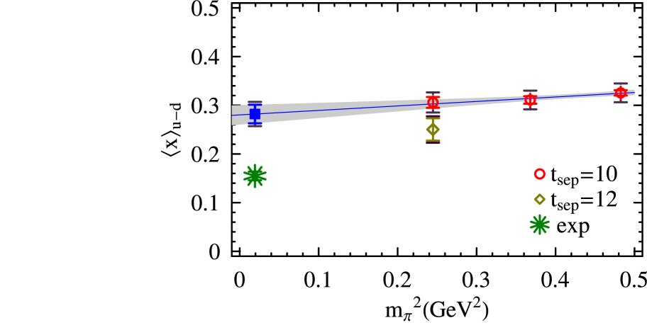
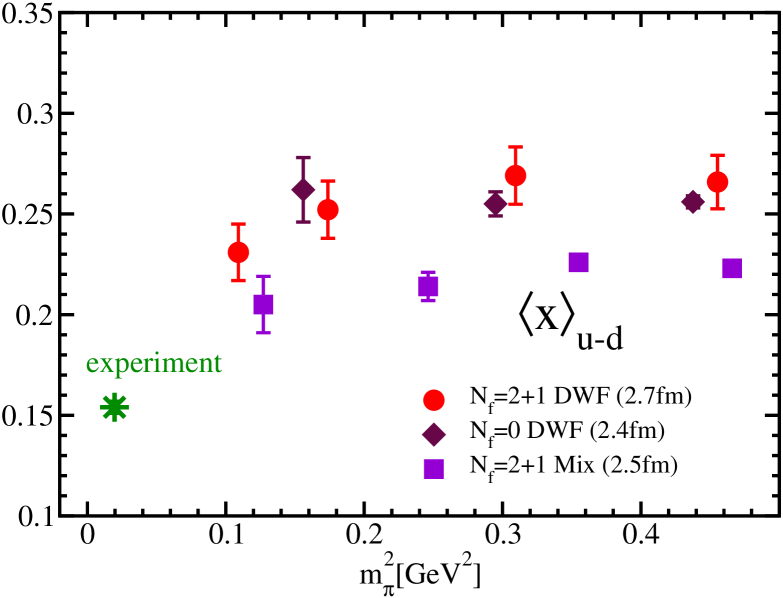
Figure 75: The momentum fraction of quarks in the isovector channel, from [LBO⁺08] (upper figure) and recent proceedings [OY08] (lower figure).

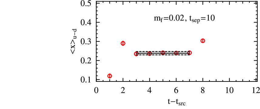
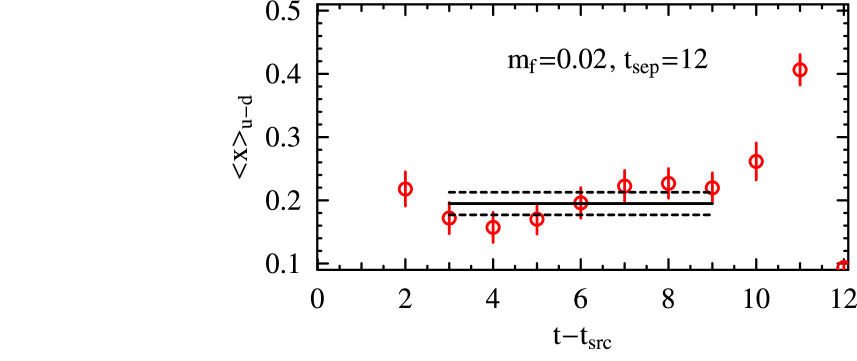
Figure 76: Plateau plots for the bare (unrenormalized) momentum fraction of quarks in the isovector channel (from [LBO⁺08]).

The situation is becoming even more challenging as soon as recent results from RBC, based on simulations with $n_{f}=2$ flavors of domain wall fermions and the DBW2 gauge action, are taken into consideration [LBO⁺08]. Results for the momentum fraction in the isovector channel that were obtained using a non-perturbatively renormalized operator, for three different pion masses of $m_{\pi}\approx 493\text{ MeV},607\text{ MeV}$ and $\approx 695\text{ MeV}$, a lattice spacing of $a\approx 0.11$ fm and a volume of $V\approx(1.9\text{ fm})^{3}$, are displayed in the upper part of Fig. 76. The lattice data points for a sink-source time separation of $(at)_{\text{sep}}=10$ (corresponding to a physical distance of $t_{\text{sep}}\sim 1.1\text{ fm}$) at $m_{\pi}\approx 493,607\text{ MeV}$ correspond to values of $\langle x\rangle^{u-d}\approx 0.31(3)_{\text{stat+ren}}$, and are therefore $\approx 50\%$ higher than the $n_{f}=2+1$ mixed action results from LHPC (Fig. 74), and $\approx 25\%$ higher than the $n_{f}=2$ clover-improved Wilson Fermion results by QCDSF (Fig. 74) at similar pion masses. Contaminations from excited states have been offered as possible explanation for this dramatic discrepancy [LBO⁺08]. At first sight, the bare momentum fraction in the upper part of Fig. 76 exhibits a perfectly flat plateau between $(at)=3$ and $(at)=7$ for the sink-source separation time of $at_{\text{sep}}=10$, thereby giving no direct indication for contributions from excited states. Nevertheless, the calculation has been repeated for a larger $at_{\text{sep}}=12$, shown in the lower part of Fig. 76. In this case, there is no clear plateau visible due to larger statistical fluctuations. However, an average over the range from $at=3$ to $at=9$ does indeed lead to a lower value for the bare momentum fraction. Consequently, a substantially lower value of $\langle x\rangle^{u-d}\approx 0.25(3)_{\text{stat+ren}}$, this time in good agreement with the results from QCDSF in Fig. 74, is obtained for $(at_{\text{sep}})=12$, as represented by the open diamond in the upper part of Fig. 76 at a pion mass of $m_{\pi}\approx 493\text{ MeV}$. It should be noted, however, that taking a simple average in the absence of a clear plateau as in, e.g., the lower part of Fig. 76, may introduce an additional systematic uncertainty. For this reason, no strong conclusions can be drawn from the above analysis at this point.

More recent results by RBC-UKQCD based on $n_{f}=2+1$ flavors of domain wall fermions and the Iwasaki gauge action, for a lattice spacing of $a\approx 0.114\text{ fm}$ in a volume of $V\approx(2.74\text{ fm})^{3}$ and pion masses ranging from $m_{\pi}\approx 331\text{ MeV}$ to $\approx 672\text{ MeV}$ are shown in the lower part of Fig. 76 [OY08]. In the range of $m_{\pi}^{2}\approx 0.2,\ldots,0.5\text{ GeV}^{2}$, these results are, in turn, $\approx 17\%$ below the $n_{f}=2$ DW results in the upper part of Fig. 76, and therefore on the same level as the $n_{f}=2$ clover-improved Wilson Fermion results by QCDSF/UKQCD in Fig. 74. A possible explanation is the larger source-sink separation of $t_{\text{sep}}=1.4\text{ fm}$ used in the case of the $n_{f}=2+1$ results in the lower part of Fig. 76, leading to a stronger suppression of contributions from excited states, which may have affected the $n_{f}=2$ DW calculation with $at_{\text{sep}}=1.1\text{ fm}$ as discussed above. One should keep in mind, however, that the quality of the signal of the two-point function at the sink, $C_{2pt}(t_{\text{snk}})$, which is used in the calculation of $\langle x\rangle$, deteriorates for large $t_{\text{snk}}$ in the case of light quark masses. The choice of a particular large source-sink separation, $t_{\text{snk}}$, may therefore be a source of an additional systematic uncertainty (see also the corresponding discussion in section 3.4.2).

Notably, the data point at the lowest pion mass in Fig. 76 exhibits a somewhat lower central value. Once the statistics has been improved, and possible systematic uncertainties like finite volume effects and fluctuations of the two-point function at large sink times are under control, this may be regarded as an encouraging sign of a bending over towards the experimental value. The $n_{f}=2+1$ mixed action results by LHPC that are displayed in Fig. 76 will be discussed in detail in section 4.4.2 below, cf. Fig. 83.

For results on individual up- and down-quark momentum fractions in quenched QCD we refer to, e.g., [G⁺96b, D⁺02, GHP⁺05] and references therein. Connected diagram contributions to individual up- and down-quark momentum fractions from simulations with dynamical quarks were presented in, e.g., [D⁺02] More recent results from LHPC [H⁺08a] on connected contributions to $\langle x\rangle^{u+d}$ will be discussed in some more detail below in section 4.4.3. Interesting attempts to finally get quark line disconnected contributions to hadron structure observables under control will be presented separately in section 6.0.2.

Unpolarized gluon momentum fraction

A first preliminary lattice study of the longitudinal momentum carried by the gluons in the nucleon was already presented more that 10 years ago in the quenched approximation using the Wilson action [G⁺97b]. The gluon momentum fraction in the nucleon is given by $\langle P|\mathcal{O}_{g}^{\mu\nu}|P\rangle=2P^{\mu}P^{\nu}\langle x\rangle^{g}$ with $\mathcal{O}_{g}^{\mu\nu}=\text{Tr}F^{\mu\alpha}(0)F^{\alpha\nu}(0)$, which corresponds directly to the pure gauge part of the QCD energy momentum tensor, $T_{g}^{\mu\nu}$. Results were presented for a perturbatively renormalized, traceless symmetric operator similar to Eq. (144), given by $\mathcal{O}_{b}=\text{Tr}\{\mathbf{E}^{2}-\mathbf{B}^{2}\}$. In order to overcome the expected noise from short-range fluctuations, a large number of up to $3500$ quenched Wilson gauge configurations were employed. Using a standard ratio of nucleon three- to two-point functions, averaged over the operator insertion time $\tau$ (keeping $\tau$ at a distance of $\delta t=4$ to source and sink), clearly non-vanishing contributions were observed for the individual chromo-electric and magnetic contributions, which however canceled out to a large extent in $\mathcal{O}_{b}$. An average value of $\langle x\rangle^{g}\approx 0.5$ with an error of $\approx 50\%$ was obtained for the three different hopping parameters $\kappa=0.1550,0.1530,0.1515$ at a lattice scale of $a^{-1}\approx 2\text{ GeV}$, corresponding to pion masses of $m_{\pi}\approx 600,850,1000\text{ MeV}$.

More recently, the $\chi$QCD collaboration extended their studies of disconnected contributions in the quark sector to include the gluon momentum fraction in the nucleon [D⁺08b]. Some details of their approach to so-called disconnected insertions (DIs) based on all-to-all quark propagators obtained from stochastic sources will be presented below in section 6.0.2 (for a brief introduction to stochastic methods, see section 2.3.3). In order to reduce the short-range fluctuations of the gluon operator, the overlap Dirac operator, $D_{\text{ov}}$, which is non-ultralocal and therefore may help to efficiently filter the ultraviolet modes, was used in the construction of a discretized field strength tensor, $F^{\text{ov}}_{\mu\nu}\propto\text{Tr}[\sigma_{\mu\nu}D_{\text{ov}}]$. That this is indeed a valid identification has been shown explicitly before in [LAH08]. The overlap Dirac operator was estimated numerically using space-time diluted $Z(4)$ noise vectors. Based on only $500$ quenched Wilson configurations, but including a large number of nucleon sources, and employing (unrenormalized) non-diagonal operators of the type $\mathcal{O}_{g}^{4i}$, a non-zero signal was observed for $\langle x\rangle^{g}$ for a pion mass of $\approx 650\text{ MeV}$. Once the gluon operators have been (non-perturbatively) renormalized, and the signals improved with the help of noise reduction techniques, these calculations may provide very interesting insights into the nucleon momentum sum rule Eq. 68.

Higher moments of the unpolarized quark PDF

Results for higher moments of the unpolarized quark distribution, $\langle x^{n-1}\rangle_{q}$, with $n=3,4$, obtained in the quenched approximation, can be found in [G⁺96b, D⁺02] based on perturbatively, and in [GHP⁺05] based on non-perturbatively renormalized operators. The LHPC-SESAM collaboration has calculated higher moments based on $n_{f}=2$ flavors of Wilson fermions, for rather large pion masses in the range of $m_{\pi}=\approx 700\text{ MeV}$ to $\approx 900\text{ MeV}$, a lattice spacing of $\approx 0.1\text{ fm}$ and a volume of $V\approx(1.6\text{ fm})^{3}$ [D⁺02]. Results from unquenched simulations at lower pion masses were to this date only presented in [G⁺05a] for $\langle x^{2}\rangle_{u-d}$ and $\langle x^{3}\rangle_{u-d}$, and data for $\langle x^{2}\rangle_{u-d,u+d}$ (only including contributions from connected diagrams) can be found in [H⁺08a]. The former were obtained for $n_{f}=2$ flavors of clover-improved Wilson fermions and pion masses down to $\approx 560\text{ MeV}$, while the latter were calculated in the framework of a hybrid calculation of $n_{f}=2+1$ flavors of domain wall valence quarks on the Asqtad MILC ensembles for $m_{\pi}\sim 350,\ldots,760\text{ MeV}$. We note that Ref. [G⁺05a] gives $\langle x^{2}\rangle_{u-d}$ and $\langle x^{3}\rangle_{u-d}$ only in the renormalization group invariant (RGI) scheme, and that the results in [H⁺08a] were obtained using (non-perturbatively improved) perturbatively renormalized operators as described in the previous section, see Eq. 140 and adjacent discussion. Since the evaluation of the nucleon three-point functions for $n=3,4$ requires non-zero hadron momenta, the signals are in general much noisier than for $n=2$ (corresponding to the momentum fractions). With this in mind, we just note that the values for $\langle x^{2}\rangle_{u-d}$ reported in quenched [GHP⁺05] and unquenched [G⁺05a] lattice QCD for $m_{\pi}\geq 550\text{ MeV}$ are $\approx 30-40\%$ larger than results from global PDF analyses, $\langle x^{2}\rangle^{\text{CTEQ6.6}}_{u-d}\simeq 0.054$ [N⁺08a] and $\langle x^{2}\rangle^{\text{MRST06}}_{u-d}\simeq 0.057$ [MSTW07]. From the same references, the lattice results for the next higher moment, $\langle x^{3}\rangle_{u-d}$, are approximately a factor of two larger in the quenched, and $\approx 30\%$ larger in the unquenched case compared to the value of $\langle x^{3}\rangle^{\text{pheno}}_{u-d}\simeq 0.023$ from the global PDF-analyses.

Moments of longitudinally polarized PDFs

In this section we review lattice calculations of the lowest moments of polarized PDFs of quarks in the nucleon, denoted by $\langle x^{n-1}\rangle_{\Delta q}$ with $n=1,2,\ldots$. The lowest moment, $n=1$, in the isovector channel is identified with the axial-vector coupling constant, $\langle x^{n-1}\rangle_{\Delta u-\Delta d}=g_{A}$, and was discussed above in section 3.4.4 in the framework of nucleon form factors.

Early studies of the polarized momentum fraction in quenched lattice QCD gave a value of $\langle x\rangle_{\Delta u-\Delta d}\approx 0.246(9)$ [G⁺97a], which is, similar to the situation for the unpolarized case discussed above, $\approx 25\%$ larger than results from phenomenology, $\langle x\rangle^{\text{pheno}}_{\Delta u-\Delta d}\simeq 0.20$ in the $\overline{\text{MS}}$-scheme at a scale of $\mu=2\text{ GeV}$ [dFSSV08]. This has been confirmed in unquenched Wilson action simulations [D⁺02], where a value of $\langle x\rangle_{\Delta u-\Delta d}\approx 0.271(25)$ was found. Both calculations were based on perturbatively renormalized operators of the form $\overline{q}\gamma_{5}\gamma_{\{\mu}{D^{\raisebox{2.41112pt}{$\scriptstyle\leftrightarrow$}}}{}_{4\}}$, with $\mu=2$ or $\mu=3$, and the cited values were obtained from a linear chiral extrapolation in $m_{\pi}^{2}$ to the physical pion mass in the $\overline{\text{MS}}$-scheme at a scale of $\mu=2\text{ GeV}$.

Recently, RBC has published results for the polarized momentum fraction based on $n_{f}=2$ flavors of domain wall fermions [LBO⁺08], obtained in the same framework as for the unpolarized momentum fraction shown in Fig. 76. The non-perturbatively renormalized operator $\overline{q}\gamma_{5}\gamma_{\{3}{D^{\raisebox{2.41112pt}{$\scriptstyle\leftrightarrow$}}}{}_{4\}}$ was employed for the analysis of $\langle x\rangle_{\Delta u-\Delta d}$, and the results, in the $\overline{\text{MS}}$-scheme at a scale of $\mu=2\text{ GeV}$, are displayed in the upper part of Fig. 78 as a function of $m_{\pi}^{2}$. As has already been observed in the previous section for $\langle x\rangle_{u-d}$, the lattice data points for a source-sink separation of $t_{\text{sep}}=10$ are found to be substantially larger than the values that were obtained in previous unquenched calculations, e.g. in [D⁺02]. Contributions from excited states have been cited as a possible cause, and the calculation has been repeated for a larger source-sink separation of $t_{\text{sep}}=12$ at the lowest pion mass of $\approx 493\text{ MeV}$. The result is represented by the open diamond in the upper part of Fig. 78, with a central value that is indeed substantially lower than for $t_{\text{sep}}=10$. However, the underlying plateau is, similar to what has been discussed in relation with $\langle x\rangle_{u-d}$ in the upper part of Fig. 76 and with Fig. 76, subject to much larger statistical noise. Furthermore, the two-point function at the sink in the ratio of three- to two-point functions may show fluctuations for large sink times. It would be important to study these issues in some more detail before more definite conclusions can be drawn from these results.

The lower part of Fig. 78 shows very recent results from RBC-UKQCD for $n_{f}=2+1$ flavors of domain wall fermions, obtained using a large source-sink separation of $at_{\text{sep}}=1.4\text{ fm}$ [OY08]. At larger pion masses, these results are $\approx 13\%$ below the $n_{f}=2$ results discussed above. We note that both the $n_{f}=2$ and $n_{f}=2+1$ DW results for $\langle x\rangle_{\Delta u-\Delta d}$ from RBC and RBC-UKQCD are substantially above the early unquenched results from [D⁺02], which may however be in parts related to the perturbative renormalization employed in the latter case. Further investigations are necessary to see if the apparent bending towards the experimental value at lower pion masses in the lower part of Fig. 78 is a physical effect due to the chiral dynamics, or rather related to the finite volume or other systematic effects.

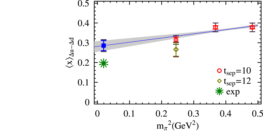
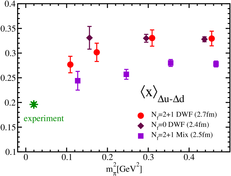
Figure 77: The polarized momentum fraction of quarks in the isovector channel from [LBO⁺08] (upper part) and the proceedings [OY08] (lower part).

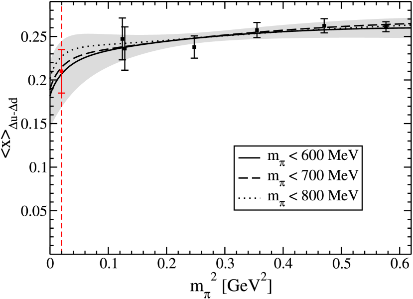
Figure 78: The polarized momentum fraction of quarks in the isovector channel (from proceedings [R⁺07]).

Figure 78 displays results from LHPC calculated in the framework of a hybrid approach with $n_{f}=2+1$ flavors of domain wall quarks and Asqtad staggered sea quarks [R⁺07], for a (non-perturbatively improved) perturbatively renormalized operator (see Eq. (140) and corresponding discussion), transformed to the $\overline{\text{MS}}$-scheme at a scale of $\mu=2\text{ GeV}$. Notably, the overall normalization, $\langle x\rangle_{\Delta u-\Delta d}\approx 0.24,\ldots,0.26$, is on the same level as the first unquenched calculations, and therefore closer to the phenomenological value than the result from RBC-UKQCD discussed above. We note, however, that the lower overall normalization may be related to the specific (partially perturbative) operator renormalization employed in this calculation. An extrapolation to the physical point, using self-consistently improved 1-loop HBChPT based on an equation similar to Eq. 148, with a different coefficient in front of the chiral logarithm, $(3g_{A,\text{lat}}^{2}+1)\rightarrow(2g_{A,\text{lat}}^{2}+1)$, was attempted. The chiral fit to the lowest four lattice data points with $m_{\pi}<600\text{ MeV}$ is represented by the shaded band in Fig. 78 and broadly overlaps within errors with the phenomenology result.

Apparently, the normalization issues in the unpolarized and polarized momentum fractions are very similar. It has been noted in this respect that a number of normalization uncertainties may be attenuated in the ratio $R=\langle x\rangle_{u-d}/\langle x\rangle_{\Delta u-\Delta d}$ [OBO06]. This ratio is not only naturally renormalized for chiral, e.g. domain wall, fermions since the renormalization constants for vector and axial-vector operators are identical in this case due to (lattice) chiral symmetry, but also the leading chiral logarithms cancel out to some extent. The latter may be, however, only relevant at very small pion masses. Interestingly, quenched and unquenched lattice results for $R$ show in general good agreement over a wide range of pion masses with the corresponding ratio from experiment and phenomenology of $R^{\exp}\approx 0.8$ at the physical point, see, e.g., [OBO06, LBO⁺08, E⁺05].

We now turn to a brief discussion of the next higher moment of the polarized quark distribution, $\langle x^{2}\rangle_{\Delta q}$. QCDSF has published a dedicated study of moments of the spin-dependent nucleon structure functions in the framework of simulations with $n_{f}=2$ flavors of clover-improved Wilson fermions [G⁺05d]. A non-perturbatively renormalized operator

$$\mathcal{O}^{5}_{214}=\overline{q}\gamma_{5}\gamma_{\{2}{D^{\raisebox{2.41112pt}{$\scriptstyle\leftrightarrow$}}}{}_{1}{D^{\raisebox{2.41112pt}{$\scriptstyle\leftrightarrow$}}}{}_{2\}}q\,,$$ (149)

where the curly brackets denote symmetrization over the respective indices, was used for the extraction of $\langle x^{2}\rangle_{\Delta q}$, which is given in the $\overline{\text{MS}}$ scheme at a scale of $5\text{ GeV}^{2}$. Results for the isovector channel are presented in Fig. 80 for pion masses in the range of $\approx 600\text{ MeV}$ to $\approx 1200\text{ MeV}$. Although there are some fluctuations visible, the lattice data points agree for all different ensembles and are practically flat in $m_{\pi}^{2}$ within statistical errors. They are on average approximately $35\%$ above the phenomenological value of $\langle x^{2}\rangle^{\text{pheno}}_{\Delta u-\Delta d}\simeq 0.065$ [dFSSV08].

These results are well compatible with the numbers obtained by LHPC based on the hybrid approach of $n_{f}=2+1$ flavors of domain wall quarks and Asqtad staggered sea quarks, displayed in Fig. 80 as a function of the ratio $(m_{\pi}/f_{\pi})^{2}$. As explained already several times before, the lattice operators have been renormalized using a non-perturbatively improved perturbative renormalization factor, cf. Eq. (140), and transformed to the $\overline{\text{MS}}$ scheme at a scale of $2\text{ GeV}$ [E⁺06b]. A chiral extrapolation based on a self-consistently improved 1-loop HBChPT formula, as discussed above in relation with $\langle x\rangle_{\Delta u-\Delta d}$, is represented by the shaded band, and agreement within errors is observed with the phenomenological value of $\langle x^{2}\rangle^{\text{pheno}}_{\Delta u-\Delta d}\simeq 0.068$ [dFSSV08] at the physical ratio $(m^{\text{phys}}_{\pi}/f^{\text{phys}}_{\pi})^{2}\approx 2.4$.

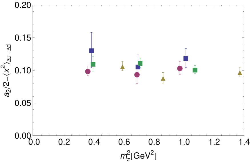
Figure 79: Higher moment of the isovector polarized quark distribution (from [G⁺05d]).

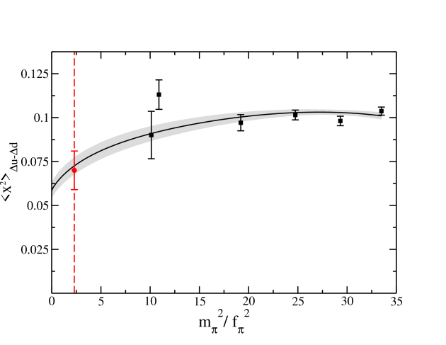
Figure 80: Higher moment of the isovector polarized quark distribution (from proceedings [E⁺06b]).

Moments of the transversity distribution

Lattice QCD results for the lowest moment of the transversity distribution, the tensor charge $\langle 1\rangle_{\delta q}=\delta q$, were discussed above in section 3.4.5. First lattice calculations of the $n=2$-moment, $\langle x\rangle_{\delta q}$, in quenched QCD and for $n_{f}=2$ Wilson fermions, based on a perturbatively renormalized operator of the form $\overline{q}\gamma_{5}\sigma_{3\{4}{D^{\raisebox{2.41112pt}{$\scriptstyle\leftrightarrow$}}}{}_{1\}}q$, were presented in [D⁺02]. Values of $\langle x\rangle_{\delta u-\delta d}\approx 0.5$ with errors of $10\%-20\%$ were reported, in the $\overline{\text{MS}}$-scheme at a scale of $\mu=2\text{ GeV}$ for pion masses of $m_{\pi}\approx 700$ and higher. We note that this is about a factor of two larger than the respective moments of the unpolarized and polarized PDFs, which are $\langle x\rangle_{u-d}\approx\langle x\rangle_{\Delta u-\Delta d}\approx 0.25$ as obtained in the same lattice study.

Substantially lower values for $\langle x\rangle_{\delta u-\delta d}$ have been reported by QCDSF in an unquenched study with $n_{f}=2$ flavors of Clover-improved Wilson quarks for pion masses in the range of $\approx 600$ to $\approx 1200\text{ MeV}$ [G⁺05g], where special care was taken that the normalization and parametrization of the corresponding nucleon matrix elements is fully consistent with the definition of moments of the transversity distribution $\delta q(x)$ [JJ91]. These calculations have been performed in the framework of an analysis of tensor GPDs and were based on the full set of non-perturbatively renormalized operators from the two 8-dimensional multiplets transforming according to the $H(4)$ representations $\tau_{1}^{(8)}$ and $\tau_{2}^{(8)}$, with typical members $\overline{q}(\sigma_{12}{D^{\raisebox{2.41112pt}{$\scriptstyle\leftrightarrow$}}}{}_{2}-\sigma_{13}{D^{\raisebox{2.41112pt}{$\scriptstyle\leftrightarrow$}}}{}_{3})q$ and $\overline{q}\sigma_{1\{2}{D^{\raisebox{2.41112pt}{$\scriptstyle\leftrightarrow$}}}{}_{4\}}q$. Results for individual up- and down-quark contributions, where only contributions from connected diagrams were taken into account, are displayed in Fig. 81 for the $\overline{\text{MS}}$-scheme at a scale of $\mu=2\text{ GeV}$. The lattice data points show a remarkable statistical precision over the full range of accessible pion masses, and are overall consistent for the different underlying ensembles, corresponding to lattice spacings in the range of $a\approx 0.07$ to $\approx 0.11\text{ fm}$ and volumes of $\approx(1.4-2.0\text{ fm})^{3}$. In the isovector channel, a value of $\langle x\rangle_{\delta u-\delta d}=0.322(6)$ was obtained from a linear chiral extrapolation in $m_{\pi}^{2}$ to the physical point [G⁺05g]. It has been speculated in [G⁺05g] that the noticeable difference between this value and the results of [D⁺02] may be related to a different normalization of the corresponding nucleon matrix elements employed in the latter work.

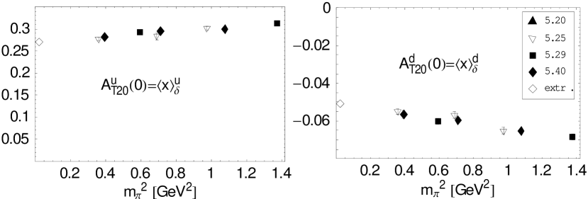
Figure 81: Up- and down-quark (connected) contributions to the $x$-moment of the transversity distribution (from [G⁺05g]).

Moments of PDFs of the $\rho$-meson

The first and only lattice QCD study of the moments of unpolarized and polarized PDFs of the $\rho$-meson was presented more than ten years ago in [B⁺97]. Calculations were performed in the quenched approximation with Wilson fermions, for three pion masses of $\approx 0.71$, $1.0$ and $1.2\text{ GeV}$, with a lattice spacing of $a\approx 0.082\text{ fm}$, calculated using the $\rho$-mass and extrapolated to the chiral limit. The study includes the moments $\langle x^{n-1}\rangle^{\rho}_{q}$ and $H_{5}^{n}$ of the unpolarized distributions $H_{1}(x)$ in Eq. 38 and $H_{5}(x)$ in Eq. 39, respectively, for $n=2,3,4$, as well as the lowest three moments $\langle x^{n-1}\rangle^{\rho}_{\Delta q}$, with $n=1,2,3$, of the polarized distribution $\widetilde{H}_{1}(x)$ in Eq. 40. Several perturbatively renormalized operators were used for the extraction of these lowest moments. Possible effects from operator mixing for $n=3,4$, corresponding to operators with two and three covariant derivatives, were not included in the analysis. The total momentum fraction carried by quarks in the rho was found to be $2\langle x\rangle^{\rho^{+}}_{u}=0.706(19)$ for $m_{\pi}\approx 1\text{ GeV}$ in the $\overline{\text{MS}}$ scheme at a scale of $\mu\approx 2.4\text{ GeV}$, approximately of the same size as for the nucleon [D⁺02] and somewhat larger than for the pion [B⁺97] in quenched QCD at similar pion masses. At the same large pion mass, a value of $\frac{1}{2}\;2\;\langle 1\rangle^{\rho^{+}}_{\Delta u}=0.702(20)$ was obtained for the total contribution of the quark spin to the spin of the rho, $S=1$. This is close to results for the nucleon in the quenched approximation [G⁺96b, D⁺02], where quarks carry approximately 65% to 70% percent of the total spin of the nucleon $S=1/2$ (see also discussion below in section 4.4.3).

4.4 Moments of GPDs

4.4.1 Moments of unpolarized GPDs of the pion

Calculations of moments of unpolarized (vector) and tensor GPDs of the pion have been performed over the last couple of years by QCDSF in unquenched lattice QCD [B⁺06e, B⁺07h, B⁺08h], however very little has so far been published in particular for the unpolarized GFFs $A^{\pi}_{ni}(t)$ for $n\geq 2$, $i=0,2,\ldots\leq n$, see, e.g., Eq. 12. We note again that the unpolarized GFF for $n=1$ is equal to the pion form factor, $A^{\pi^{+}}_{u,10}(t)=F_{\pi}(t=-Q^{2})$, for which a number of lattice results are available, see section 3.3. For a preliminary analysis of the GFFs $A^{\pi}_{20}(t)$ and $A^{\pi}_{22}(t)$ in unquenched lattice QCD, we refer to the PhD thesis by Brömmel [Brö]. Lattice QCD results for the tensor GPD of the pion, $E^{\pi}_{T}(x,\xi,t)$, Eq. (7), in the form of the lowest two moments $B_{T10}^{\pi}(t)$ and $B_{T20}^{\pi}(t)$, will be presented in the framework of a discussion of the transverse pion spin structure below in section 4.4.7.

4.4.2 Form Factors of the Nucleon Energy Momentum Tensor

The form factors of the energy momentum tensor for quarks in the nucleon, denoted by $A^{q}_{20}(t)$, $B^{q}_{20}(t)$ and $C^{q}_{20}(t)$ (see Eqs. (66) and (67)) have been studied for the first time in the quenched approximation with Wilson fermions by QCDSF [G⁺04a] for pion masses in the range of $\approx 600$ to $\approx 1000\text{ MeV}$, and at about the same time by LHPC-SESAM [H⁺03] using $n_{f}=2$ flavors of Wilson fermions and the Wilson gauge action for a pion mass of $\approx 900\text{ MeV}$.

Figure 83 displays as an example results for the generalized form factors (GFFs) $A^{u-d}_{20}(t)$, $B^{u-d}_{20}(t)$ and $C^{u-d}_{20}(t)$ as functions of the momentum transfer squared, $t$, for $m_{\pi}\approx 498\text{ MeV}$ obtained recently by LHPC in a hybrid approach based on $n_{f}=2+1$ flavors of domain wall valence and Asqtad staggered sea quarks [H⁺08a]. As has been discussed several times before, the underlying lattice operators in this analysis were renormalized perturbatively, supplemented by a non-perturbative improvement factor as given in Eq. 140, and all results were transformed to the $\overline{\text{MS}}$ scheme at a scale of $\mu=2\text{ GeV}$. The shaded bands in Fig. 83 represent dipole fits to the lattice data points for $A^{u-d}_{20}(t)$ and $B^{u-d}_{20}(t)$, and a linear fit in $t$ to $C^{u-d}_{20}(t)$.

Similar results obtained by QCDSF for $n_{f}=2$ flavors of clover-improved Wilson fermions are shown for comparison in Fig. 83 for a pion mass of $m_{\pi}\approx 350\text{ MeV}$ [B⁺07g]. Non-perturbatively renormalized lattice operators were employed for the extraction of the GFFs, which are also given in the $\overline{\text{MS}}$ scheme at a scale of $\mu=2\text{ GeV}$. Although the corresponding pion masses are different, the results in Fig. 83 and Fig. 83 are in general compatible, apart from a difference in the overall normalization of the lattice data points for $A^{u-d}_{20}(t)$ and $B^{u-d}_{20}(t)$, where the results from QCDSF are $\approx 10$ to $25\%$ above the values from LHPC. This discrepancy has already been discussed in connection with the forward value $A^{u-d}_{20}(t=0)=\langle x\rangle^{u-d}$ in Figs. 74 and 74 in section 4.3.2 above. We note in particular that the GFF $B^{u-d}_{20}(t)$ is sizeable and larger than $A^{u-d}_{20}(t)$ over the full range $-t\leq 1.3\text{ GeV}^{2}$. At the same time, one finds that the GFF $C^{u-d}_{20}(t)$ is compatible with zero within statistical errors for all accessible values of $-t\approx 0.25,\ldots,1.3\text{ GeV}^{2}$.

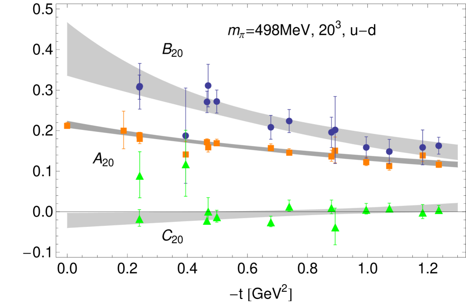
Figure 82: Form factors of the energy momentum tensor in the isovector channel (from [H⁺08a]).

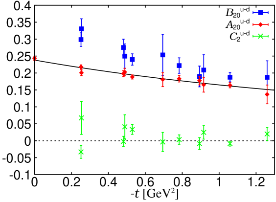
Figure 83: Form factors of the energy momentum tensor in the isovector channel (from proceedings [B⁺07g]).

In the following, we discuss the results by LHPC and QCDSF for the form factors of the energy momentum tensor in some more detail. LHPC has calculated $A^{q}_{20}(t)$, $B^{q}_{20}(t)$ and $C^{q}_{20}(t)$ for six different pion masses from $\approx 355\text{ MeV}$ to $\approx 760\text{ MeV}$, with a lattice spacing of $a\approx 0.124\text{ fm}$, for a volume of $\approx(2.5\text{ fm})^{3}$ [H⁺08a]. The calculations at the lowest pion mass were repeated in a larger volume of $\approx(3.5\text{ fm})^{3}$, allowing to check for possible finite volume effects. The forward value $A^{u-d}_{20}(t=0)=\langle x\rangle^{u-d}$ is shown in Fig. 85 as a function of $m_{\pi}^{2}$. These results differ from the results for the momentum fraction of $u-d$ quarks presented in Fig. 74 only in the number of lattice operators that were included in the respective analyses. While the lattice data points in Fig. 74 were obtained using the operator in Eq. 144, the results in Fig. 85 were based on the complete set of symmetric and traceless lattice operators transforming according to the irreducible representations $\tau_{1}^{(3)}$ and $\tau_{1}^{(6)}$ of dimensions three and six, respectively [G⁺96a]. The good agreement of the lattice data points at $m_{\pi}\approx 355\text{ MeV}$ for the two different volumes, represented by the open and filled circles in Fig. 85, indicates that finite volume effects are small compared to the statistical errors, at least at this particular pion mass.

A chiral extrapolation of the GFFs $A^{u-d}_{20}(t)$, $B^{u-d}_{20}(t)$ and $C^{u-d}_{20}(t)$ was attempted using recent results obtained in the framework of a covariant baryon ChPT (CBChPT) calculation to $\mathcal{O}(p^{2})$ [DGH08]. The $m_{\pi}$- and $t$-dependences of the GFFs are given by

$$A_{20}^{u-d}(t,m_{\pi}) = A_{20}^{0,u-d}\bigg{(}f_{A}^{u-d}(m_{\pi})+\frac{(g^{0}_{A})^{2}}{192\pi^{2}(f^{0}_{\pi})^{2}}h_{A}(t,m_{\pi})\bigg{)}+\langle x\rangle^{0}_{\Delta u-\Delta d}j_{A}^{u-d}(m_{\pi})$$ (150)

$$+ \delta_{A}^{t,u-d}\,t+\delta_{A}^{m_{\pi},u-d}\,m_{\pi}^{2}\,,$$

$$B_{20}^{u-d}(t,m_{\pi})=\frac{m_{N}(m_{\pi})}{m^{0}_{N}}B_{20}^{0,u-d}+A_{20}^{0,u-d}h_{B}^{u-d}(t,m_{\pi})+\frac{m_{N}(m_{\pi})}{m^{0}_{N}}\bigg{(}\delta_{B}^{t,u-d}\,t+\delta_{B}^{m_{\pi},u-d}\,m_{\pi}^{2}\bigg{)}\,,$$ (151)

$$C_{20}^{u-d}(t,m_{\pi})=\frac{m_{N}(m_{\pi})}{m^{0}_{N}}C_{20}^{0,u-d}+A_{20}^{0,u-d}h_{C}^{u-d}(t,m_{\pi})+\frac{m_{N}(m_{\pi})}{m^{0}_{N}}\bigg{(}\delta_{C}^{t,u-d}\,t+\delta_{C}^{m_{\pi},u-d}\,m_{\pi}^{2}\bigg{)}\,.$$ (152)

Apart from the axial-vector coupling and the pion decay constant in the chiral limit, which were fixed to $g_{A}^{0}=1.2$ and $f_{\pi}^{0}=0.092\text{ GeV}$, Eqs. (150,151,152) depend on 10 additional LECs: The chiral limit values of the GFFs at $t=0$, $F_{20}^{0,u-d}=F_{20}^{u-d}(t\text{{=}}0,m_{\pi}\text{{=}}0)$, the counter-terms $\delta_{F}^{t,u-d}$ and $\delta_{F}^{m_{\pi},u-d}$, all with $F=A,B,C$, and the polarized momentum fraction in the chiral limit, $\langle x\rangle^{0}_{\Delta u-\Delta d}$. The latter was fixed to $\langle x\rangle^{0}_{\Delta u-\Delta d}=0.17$ as obtained from the self-consistently improved chiral extrapolation in Fig. 78 [E⁺06b]. Explicit expressions for the functions $f_{A}^{u-d}(m_{\pi})$, $h_{F}(t,m_{\pi})$ and $j_{A}^{u-d}(m_{\pi})$, which contain the non-analytic dependences on the momentum transfer squared and the pion mass, can be found in [DGH08]. It turns out that the functions $h_{F}(t,m_{\pi})$ are practically independent of $t$ in the accessible ranges of $t$ and $m_{\pi}$. The counter terms $\delta_{F}^{t,u-d}$ and $\delta_{F}^{m_{\pi},u-d}$ for $F=B,C$ included in the fit are formally of $\mathcal{O}(p^{3})$ and therefore represent parts of higher order corrections. Since the extraction of the GFFs was based on the parametrization in Eq. 66 using the lattice values for the nucleon mass $m_{N}$, the ratio $m_{N}(m_{\pi})/m^{0}_{N}$ of the pion mass dependent nucleon mass to the nucleon mass in the chiral limit, which has been fixed to $m^{0}_{N}=0.89\text{ GeV}$, appears in Eqs. (151) and (152).

We note in particular that Eqs. (150,151) and (152) depend simultaneously on the momentum fraction in the isovector channel in the chiral limit, $A_{20}^{0,u-d}=\langle x\rangle^{0}_{u-d}$. For this reason, a global simultaneous chiral fit to the $t$- and $m_{\pi}$-dependence of the GFFs $A^{u-d}_{20}(t)$, $B^{u-d}_{20}(t)$ and $C^{u-d}_{20}(t)$ was performed including nine free parameters: The LECs $F_{20}^{0,u-d}$, and the counter-terms $\delta_{F}^{t,u-d}$ and $\delta_{F}^{m_{\pi},u-d}$, for $F=A,B,C$. To improve the statistics, all lattice results for $-t<0.48\text{ GeV}^{2}$ and $m^{2}_{\pi}\leq 500^{2}\text{ MeV}^{2}$ were included in the fit, amounting to more than 120 lattice data points. The maximal values for the pion mass and the momentum transfer that were taken into account in the chiral fit appear to be rather large and are probably beyond the commonly anticipated region of applicability of a $\mathcal{O}(p^{2})$-CBChPT calculation. The stability of the fit has already been checked in [H⁺08a] to some extent by lowering the maximal values of included pion masses down to $500\text{ MeV}$, and a consistent description of $A^{u-d}_{20}(t=0)$ within errors was obtained in all studied cases. Still, it would be important to investigate the issue of convergence of the chiral expansions of all three GFFs in greater detail in future studies.

The result of the global simultaneous chiral fit just described is represented by the shaded bands in Figs. 85, 85, 87 and 87. A value of $A_{20}^{u-d}(t\text{{=}}0)=\langle x\rangle_{u-d}=0.157(10)$ was obtained at the physical point, in very good agreement with results from global PDF-analyses, e.g. the MRST and CTEQ PDF parametrizations, $\langle x\rangle^{\text{CTEQ6.6}}_{u-d}=0.154$ and $\langle x\rangle^{\text{MRST06}}_{u-d}=0.158$ [MSTW07, N⁺08a], represented by the star in Fig. 85.

The dotted line in Fig. 85 represents the heavy baryon limit, $m_{N}\rightarrow\infty$, of the CBChPT fit. If the CBChPT fit describes the physics correctly, then the early breakdown of the heavy-baryon limit curve strongly suggest that the tower of terms $\propto(m_{\pi}/m_{N})^{n}$ included in the covariant approach is essential for a successful description of the lattice data beyond the physical point. However, it is interesting to note that a direct fit of the corresponding HBChPT formula for $\langle x\rangle_{u-d}$ [AS02, CJ01] to the lattice data for $m_{\pi}<500\text{ MeV}$, as represented by the dashed line, misses the value from phenomenology&experiment only by about $10\%$.

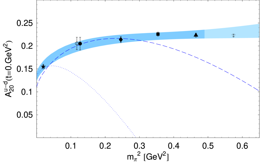
Figure 84: Pion mass dependence and chiral extrapolation of $\langle x\rangle_{u-d}=A_{20}^{u-d}(t=0)$ (from [H⁺08a]).

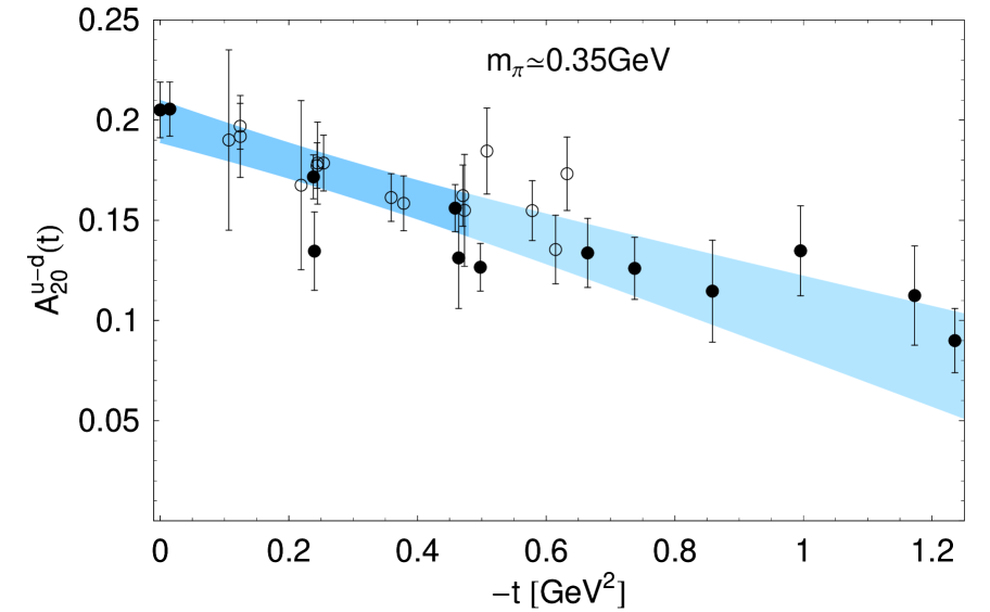
Figure 85: Dependence of $A_{20}^{u-d}(t)$ on the squared momentum transfer $t$ for a pion mass of $\approx 350\text{ MeV}$ (from [H⁺08a]).

Figure 85 shows the lattice results for $A_{20}^{u-d}(t)$ at a pion mass of $\approx 355\text{ MeV}$, together with the chiral extrapolation, versus the momentum transfer squared. Apparently, the almost linear dependence on $t$ obtained from the chiral fit is in good agreement with the lattice results for $-t<1\text{ GeV}^{2}$ within statistical errors.

The pion mass dependences of the GFFs $B_{20}^{u-d}(t)$ and $C_{20}^{u-d}(t)$ for fixed $t\simeq-0.24\text{ GeV}^{2}$ are displayed in Figs. 87 and 87, respectively. In both cases, the lattice data points are described reasonably well by the CBChPT fit, albeit the rather large statistical errors preclude any strong conclusions. A clearly non-zero value is obtained for $B_{20}^{u-d}$ in the forward limit at the physical pion mass, $B_{20}^{u-d}(t\text{{=}}0)=0.273(63)$, while the chiral fit gives a value for $C_{20}^{u-d}$ that is compatible with zero within errors over the full range of accessible pion masses and values of the momentum transfer, with $C_{20}^{u-d}(t\text{{=}}0)=-0.017(41)$ at $m_{\pi}=0.140\text{ MeV}$.

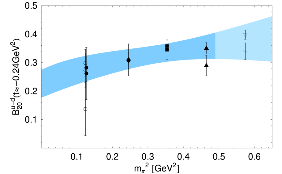
Figure 86: Pion mass dependence and chiral extrapolation of $B_{20}^{u-d}(t\simeq 0.24\text{ GeV}^{2})$ (from [H⁺08a]).

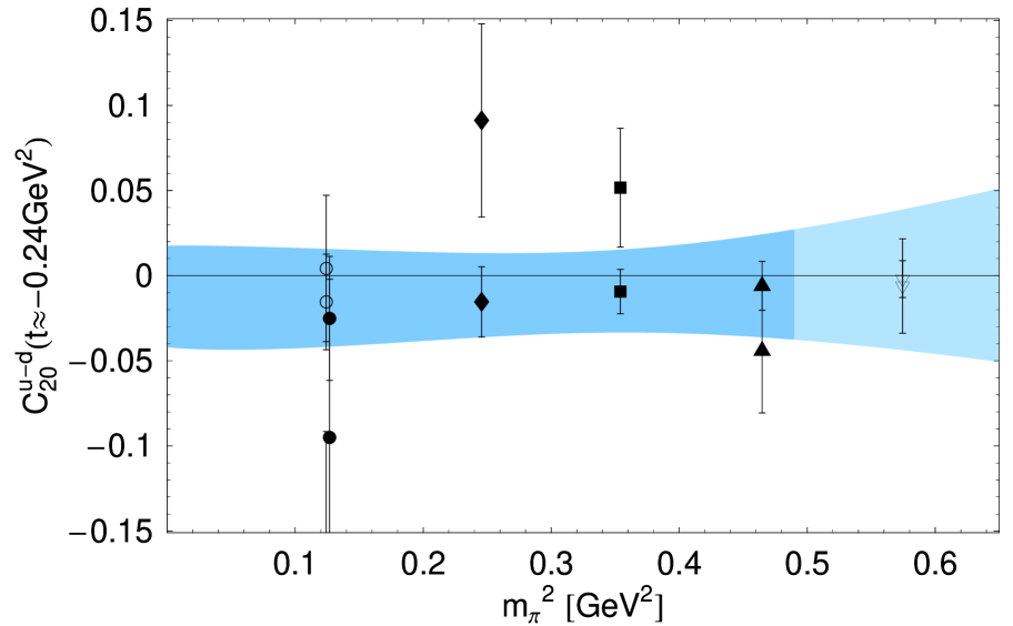
Figure 87: Pion mass dependence and chiral extrapolation of $C_{20}^{u-d}(t\simeq 0.24\text{ GeV}^{2})$ (from [H⁺08a]).

Corresponding results for $A^{u-d}_{20}(t\text{{=}}0)$ and $B^{u-d}_{20}(t\text{{=}}0)$ from the QCDSF collaboration for $n_{f}=2$ flavors of clover-improved Wilson fermions are presented in Figs. 89 and 89 as functions of the squared pion mass [B⁺07g]. The shaded band in Fig. 89 represents a chiral fit based on Eq. (150) at fixed $t=0$ with two parameters $A_{20}^{0,u-d}=\langle x\rangle^{0}_{u-d}$ and $\delta_{A}^{m_{\pi},u-d}$ to the lattice data points for $m_{\pi}\leq 700\text{ MeV}$. Due to the higher normalization of the data points compared to Fig. 85, a value of $A_{20}^{u-d}(t\text{{=}}0)=\langle x\rangle_{u-d}=0.198(8)$ was found at the physical pion mass, which is $\approx 25\%$ larger than the phenomenological PDF-parametrizations would suggest.

Employing Eq. (151), a chiral fit with three parameters $B_{20}^{0,u-d}$, $\delta_{B}^{t,u-d}$ and $\delta_{B}^{m_{\pi},u-d}$ was performed to the lattice data for $B^{u-d}_{20}(t)$ for $m_{\pi}\leq 700\text{ MeV}$. Since the GFFs $A^{u-d}_{20}$ and $B^{u-d}_{20}$ were not fitted simultaneously, the LEC $A_{20}^{0,u-d}(t\text{{=}}0)$ in Eq. (151) was fixed to the value obtain from the fit in Fig. 89. Figure 89 shows the results of the fit for vanishing momentum transfer as a function of $m_{\pi}^{2}$ as shaded band, and the displayed data points are the result of an extrapolation of the lattice data to $t=0$ using the fitting formula. A value of $B^{u-d}_{20}(t\text{{=}}0)=0.269(20)$ was found at the physical point, which is in good agreement with the results from LHPC discussed above.

While the description of the lattice data points for $A^{u-d}_{20}(t\text{{=}}0)$ and $B^{u-d}_{20}(t\text{{=}}0)$ by the CBChPT extrapolations in Figs. 89 and 89 is quite satisfactory at lower pion masses, the fit bands start to bend down and thus do not follow the trend of the lattice results for $m_{\pi}>700\text{ MeV}$. It would be interesting to investigate the stability of these chiral extrapolations by restricting the ranges of $m_{\pi}$ and $t$ included in the fit, and by considering simultaneous global fits to all three GFFs $A^{q}_{20}(t)$, $B^{q}_{20}(t)$ and $C^{q}_{20}(t)$ as discussed above.

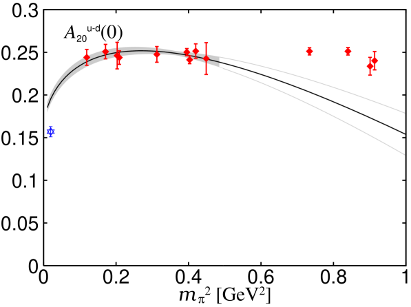
Figure 88: Pion mass dependence and chiral extrapolation of $\langle x\rangle_{u-d}=A_{20}^{u-d}(t\text{{=}}0)$ (from proceedings [B⁺07g]).

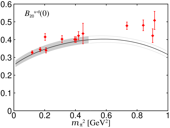
Figure 89: Pion mass dependence and chiral extrapolation of $B_{20}^{u-d}(t\text{{=}}0)$ (from proceedings [B⁺07g]).

We now turn to a discussion of the energy momentum tensor form factors in the isosinglet channel. All results presented in the remainder of this section correspond only to quark line connected diagrams. Disconnected contributions, which are required to obtain the full isosinglet results, were not included so far. Exemplary results for $A^{u+d}_{20}(t)$, $B^{u+d}_{20}(t)$ and $C^{u+d}_{20}(t)$ from LHPC for a pion mass of $\approx 498\text{ MeV}$, based on the same lattice approach and ensembles as discussed at the beginning of this section, is presented in Fig. 91 [H⁺08a]. While the GFF $A^{u+d}_{20}(t)$ is rather large and positive over the full range of $t$, the values for $C^{u+d}_{20}(t)$ are clearly negative (albeit with larger statistical fluctuations), and one finds in particular that the GFF $B^{u+d}_{20}(t)$ is compatible with zero within statistical errors for all accessible values of $t$. In comparison with the isovector channel displayed in Fig. 91, we note that $A^{u+d}_{20}>A^{u-d}_{20}$, $B^{u-d}_{20}\gg B^{u+d}_{20}$, and $|C^{u+d}_{20}|\gtrapprox|C^{u-d}_{20}|$. These results are in overall agreement with counting rules for GPDs obtained in the framework of an expansion in $1/N_{c}$ [GPV01], which predict that $(A^{u-d}_{20}/A^{u+d}_{20},B^{u+d}_{20}/B^{u-d}_{20},C^{u-d}_{20}/C^{u+d}_{20})\sim 1/N_{c}$.

The dependence on the pion mass and the momentum transfer of the GFFs in the isosinglet channel in CBChPT [DGH08] is given by

$$A_{20}^{u+d}(t,m_{\pi})=A_{20}^{0,u+d}\bigg{(}f^{u+d}_{A}(m_{\pi})-\frac{g_{A}^{2}}{64\pi^{2}f_{\pi}^{2}}h_{A}(t,m_{\pi})\bigg{)}+\delta_{A}^{t,u+d}\,t+\delta_{A}^{m_{\pi},u+d}\,m_{\pi}^{2}+\Delta A_{20}^{u+d}(t,m_{\pi})\,,$$ (153)

$$B_{20}^{u+d}(t,m_{\pi}) = \frac{m_{N}(m_{\pi})}{m_{N}}B_{20}^{0,u+d}+A_{20}^{0,u+d}h_{B}^{u+d}(t,m_{\pi})+\Delta B_{20}^{u+d}(t,m_{\pi})$$ (154)

$$+ \frac{m_{N}(m_{\pi})}{m_{N}}\bigg{\{}\delta_{B}^{t,u+d}\,t+\delta_{B}^{m_{\pi},u+d}\,m_{\pi}^{2}\bigg{\}}\,,$$

$$C_{20}^{u+d}(t,m_{\pi}) = \frac{m_{N}(m_{\pi})}{m_{N}}C_{20}^{0,u+d}+A_{20}^{0,u+d}h_{C}^{u+d}(t,m_{\pi})+\Delta C_{20}^{u+d}(t,m_{\pi})$$ (155)

$$+ \frac{m_{N}(m_{\pi})}{m_{N}}\bigg{\{}\delta_{C}^{t,u+d}\,t+\delta_{C}^{m_{\pi},u+d}\,m_{\pi}^{2}\bigg{\}}\,,$$

where the functions $f_{A}^{u+d}(m_{\pi})$, $h_{F}(t,m_{\pi})$ and $\Delta F_{20}^{u+d}(t,m_{\pi})$, with $F=A,B,C$, contain the non-analytic dependences on the momentum transfer squared and the pion mass. We note that the terms $\Delta F_{20}^{u+d}(t,m_{\pi})$, $\delta_{B}^{t,u+d}\,t$, $\delta_{B}^{m_{\pi},u+d}\,m_{\pi}^{2}$ represent only specific parts of the full $\mathcal{O}(p^{3})$ corrections [DGH08], and that the counter-terms $\delta_{C}^{t,u+d}\,t$ and $\delta_{C}^{m_{\pi},u+d}\,m_{\pi}^{2}$ formally appear only at $\mathcal{O}(p^{4})$ in the chiral expansion and were added by hand in Eq. (155). The chiral extrapolation formulas depend on the LECs $F_{20}^{0,u+d}=F_{20}^{u+d}(t\text{{=}}0,m_{\pi}\text{{=}}0)$ and the counter-terms $\delta_{F}^{t,u+d}$ and $\delta_{F}^{m_{\pi},u+d}$. Furthermore, the $\mathcal{O}(p^{3})$-correction terms $\Delta F_{20}^{u+d}(t,m_{\pi})$ are all proportional to another LEC, the total momentum fraction of quarks in the pion in the chiral limit, $\langle x\rangle^{\pi,0}_{u+d}$, which was fixed to $0.5$, as suggested by phenomenology and the lattice studies mentioned in section 4.3.1.

Preliminary fits to the lattice data for $B_{20}^{u+d}$ turned out to be unstable due to unreasonably large contributions from the term $\Delta B_{20}^{u+d}(t,m_{\pi})$ in Eq. 154, which subsequently was excluded from the full chiral analysis [H⁺08a]. Noting that $A_{20}^{0,u+d}=\langle x\rangle^{0}_{u+d}$ is a common LEC in the chiral expansions in Eqs. (153,154,155), LHPC has performed a simultaneous global chiral fit to more than 120 lattice data points for $A^{u+d}_{20}(t)$, $B^{u+d}_{20}(t)$ and $C^{u+d}_{20}(t)$, with $m^{2}_{\pi}<500\text{ MeV}^{2}$ and $|t|<0.48\text{ GeV}^{2}$, including the 9 free parameters $\Delta F_{20}^{u+d}(t,m_{\pi})$, $\delta_{F}^{t,u+d}\,t$ and $\delta_{F}^{m_{\pi},u+d}\,m_{\pi}^{2}$.

Figure 91 displays the lattice data from LHPC for $A^{u+d}_{20}(t\text{{=}}0)$ versus $m_{\pi}^{2}$ together with the result of the chiral fit represented by the shaded band. An upwards bending of the chiral extrapolation band is visible at lower pion masses, which leads to a value of $A_{20}^{u+d}(t\text{{=}}0)=\langle x\rangle_{u+d}=0.520(24)$ at the physical pion mass that is in a good agreement with global PDF-parametrizations, $\langle x\rangle^{\text{MRST06}}_{u+d}=0.545$ and $\langle x\rangle^{\text{CTEQ6.6}}_{u+d}=0.535$ [MSTW07, N⁺08a]. It has been noted, however, that the term $\Delta A_{20}^{u+d}(t,m_{\pi})$ in Eq. 153, which represent only part of the full $\mathcal{O}(p^{3})$ correction, is mainly responsible for the observed upward bending. Furthermore, the inclusion of disconnected contributions could not only change the normalization but also the pion mass and $t$-dependence of the lattice data, and therefore could lead to a different chiral fit. Hence the extrapolation in Fig. 91 and in particular the good agreement with the PDF parametrizations should be considered with great caution, at least until the complete $\mathcal{O}(p^{3})$ ChPT results become available and can be used in fits to lattice data, including contributions from disconnected diagrams.

Similar concerns apply to the results for the GFF $B_{20}^{u+d}$, which are shown in Fig. 93 for fixed $t\simeq-0.24\text{ GeV}^{2}$ versus $m_{\pi}^{2}$. The lattice data points are well described by the chiral extrapolation band, which bends down towards negative values at small pion masses. In the forward limit, the fit gives $B^{u+d}_{20}(t\text{{=}}0)=-0.140(84)$ at the physical pion mass. As before, the full $\mathcal{O}(p^{3})$ corrections on the side of ChPT and disconnected contributions on the side of the lattice calculation must be included before this can be regarded as a solid result.

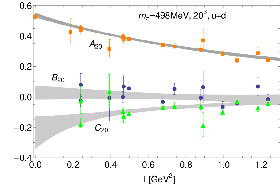
Figure 90: Connected contributions to the form factors of the energy momentum tensor in the isosinglet channel (from [H⁺08a]).

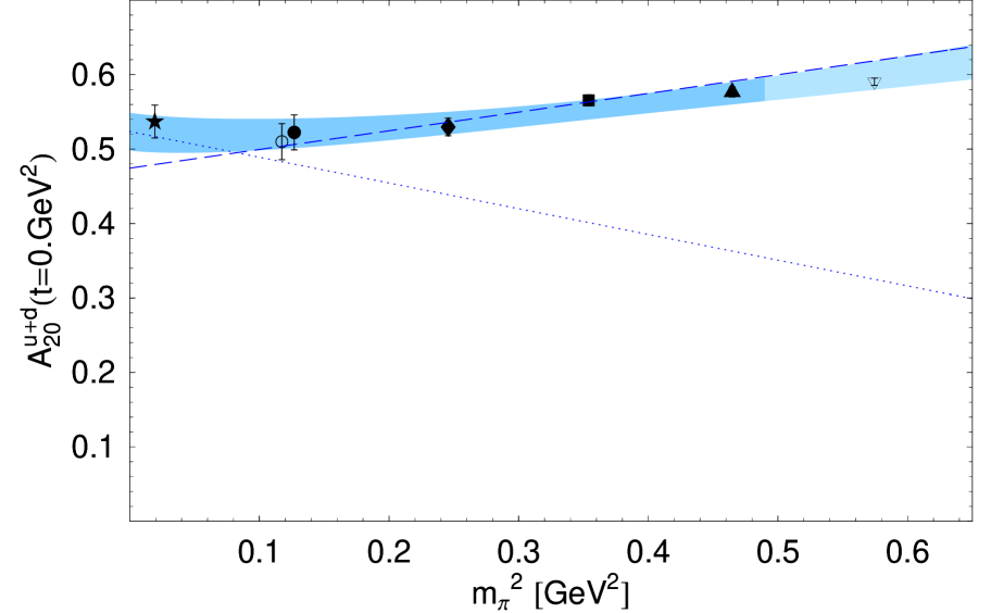
Figure 91: Pion mass dependence and chiral extrapolation of connected contributions to $\langle x\rangle_{u+d}=A_{20}^{u+d}(t\text{{=}}0)$ (from [H⁺08a]).

Figure 93 displays the simultaneous pion mass and $t$-dependence of the lattice results for the GFF $C_{20}^{u+d}$, together with the simultaneous global chiral fit. The lattice data points and their statistical errors are represented by the elongated cuboids, the central result from the chiral extrapolation is given by the surface, and the statistical errors from the fit are illustrated by the error bands at $t=0$ and $m_{\pi}=0$. From the chiral fit, a sizeable negative value of $C^{u-d}_{20}(t\text{{=}}0)=-0.267(62)$ was found at the physical pion mass. Similar comments as made above for $A^{u+d}_{20}$ and $B^{u+d}_{20}$ regarding the reliability of the chiral extrapolation apply also in this case.

Results from QCDSF for the isosinglet GFFs $A^{u+d}_{20}$ and $B^{u+d}_{20}$ are presented in Figs. 95 and 95, based on the same simulations and ensembles as discussed above in relation with Figs. 89 and 89 [B⁺07g]. As in the case of the LHPC simulations, contributions from disconnected diagrams were not yet included. Notably, the normalization of the lattice data points for $A^{u+d}_{20}$ in Fig. 95 is $\approx 10\%$ higher than of the corresponding results from LHPC in Fig. 91. A chiral fit based on Eq. 153 at fixed $t=0$ and excluding the $\mathcal{O}(p^{3})$ correction term $\Delta A_{20}^{u+d}(t,m_{\pi})$, with two free parameters $A_{20}^{0,u+d}=\langle x\rangle^{0}_{u+d}$ and $\delta_{B}^{m_{\pi},u+d}$, is represented by the solid lines and the shaded band. The chiral fit smoothly bends down as $m_{\pi}\rightarrow 0$, giving $A_{20}^{u+d}=\langle x\rangle_{u+d}=0.572(12)$ at the physical point, which is approximately $6\%$ above the values from phenomenological PDF parametrizations. Since the term $\Delta A_{20}^{u+d}(t,m_{\pi})$ was not included in the fit, there is no upwards bending visible at low pion masses as seen in Fig. 91. This confirms that the full $\mathcal{O}(p^{3})$ corrections have to be worked out in CBChPT and applied to the lattice results before any definite conclusions can be drawn.

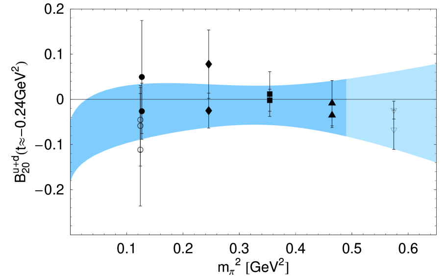
Figure 92: Pion mass dependence and chiral extrapolation of connected contributions to $B_{20}^{u+d}(t\simeq-0.24\text{ GeV}^{2})$ (from [H⁺08a]).

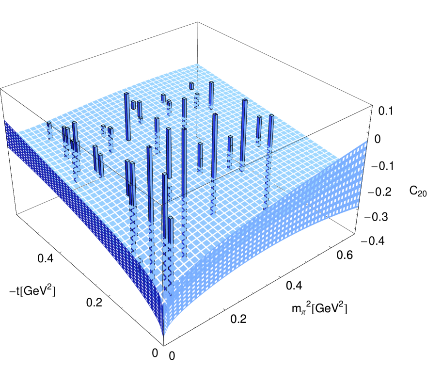
Figure 93: Pion mass and $t$-dependence together with a chiral extrapolation of connected contributions to $C_{20}^{u+d}(t)$ (from [H⁺08a]).

Equation (154), with $\Delta B_{20}^{u+d}(t,m_{\pi})$ set to zero, was used to fit the lattice data for $B^{u+d}_{20}(t)$, treating $B^{0,u+d}_{20}$, $\delta_{B}^{t,u+d}$ and $\delta_{B}^{m_{\pi},u+d}$ as free parameters, and setting the LEC $A_{20}^{0,u+d}=\langle x\rangle^{0}_{u+d}$ to the value obtained from the fit in Fig. 95. The result is shown as shaded band in Fig. 95, where the lattice data points have already been extrapolated to $t=0$ at fixed $m_{\pi}$ based on the chiral fit. From the chiral extrapolation, a value of $B^{u+d}_{20}(t\text{{=}}0)=-0.120(23)$ was obtained at the physical pion mass [B⁺07g], in good agreement with the result from LHPC based on the simultaneous global fit discussed above. Since contributions from disconnected diagrams and the full $\mathcal{O}(p^{3})$ CBChPT corrections were not included, these results should be considered with appropriate caution.

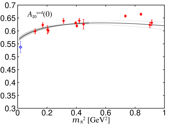
Figure 94: Pion mass dependence and chiral extrapolation of connected contributions to $\langle x\rangle_{u+d}=A_{20}^{u+d}(t\text{{=}}0)$ (from proceedings [B⁺07g]).

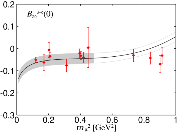
Figure 95: Pion mass dependence and chiral extrapolation of connected contributions to $B_{20}^{u+d}(t\text{{=}}0)$ (from proceedings [B⁺07g]).

4.4.3 Nucleon spin structure

A central role in our understanding of the spin structure of the nucleon is played by the total quark spin contribution $\Delta\Sigma=\sum_{q=u,d,s}\Delta q$, cf. Eq. (75). Early experimental results by EMC suggested a very small value (albeit with rather large errors) of $\Delta\Sigma\simeq 0.098\pm 0.136$ [A⁺89] at a scale of $\approx 10\text{ GeV}^{2}$, which triggered the famous “proton spin crisis”. From a recent precise measurement of the spin structure functions at HERMES [A⁺07b], a value of $\Delta\Sigma=\sum_{q=u,d,s}\Delta q=0.330(11)_{\text{th}}(25)_{\text{exp}}(28)_{\text{evo}}$ has been extracted for the $\overline{\text{MS}}$ scheme at a scale of $5\text{ GeV}^{2}$. These results strongly indicate that the major fraction of the total nucleon spin is indeed carried by the gluon spin and the orbital angular momentum contributions of quarks and gluons.

Pioneering studies of $\Delta\Sigma$ in quenched lattice QCD were presented in [FKOU95, DLL95]. In both cases, perturbatively renormalized operators were employed, and values of $\Delta\Sigma=0.18(10)$ [FKOU95] and $\Delta\Sigma=0.25(12)$ [DLL95] (see also Table 1 below) were cited at lattice scales of $\mu=1/a\approx 1.4\text{ GeV}$, including estimates of the disconnected contributions for $q=u,d,s$. A similar value of $\Delta\Sigma=0.20(12)$ was presented in [G⁺99b], for $n_{f}=2$ flavors of Wilson fermions and the Wilson gauge action, and based on a perturbatively renormalized operator. As in the earlier quenched studies, estimates of disconnect contributions using stochastic noise methods were also included in this case. More recent results for the connected contributions to $\Delta\Sigma^{u+d}$ from unquenched lattice QCD will be presented and discussed further below in this section, cf. Figs. 97 to 100.

Together with the relations discussed in section 2.1.6, in particular Eq. (70), the results for the GFFs $A^{q}_{20}$ and $B^{q}_{20}$ in the isovector and isosinglet channel from the previous section can now be used to study the quark angular momentum, $J^{q}$, contributions to the nucleon spin $1/2$, Eqs. (69,75). Furthermore, taking into account the results for the quark spin contributions, $\Delta\Sigma^{q}$, which was for the isovector case (identifying $\Delta\Sigma^{u-d}=g^{(3)}_{A}$) already discussed in section 3.4.4, we also gain access to the orbital angular momentum, $L^{q}$, carried by the quarks in the nucleon, as defined in Eq. (72).

Before going into the details of the recent results obtained by LHPC and QCDSF in unquenched lattice QCD, we note that a first study of the angular and orbital angular momentum contributions to the spin of the nucleon was performed in the quenched approximation in [MDL⁺00]. In this work, the sum $T^{q}(t)\equiv(A^{q}_{20}(t)+B^{q}_{20}(t))/2$, for three different non-zero values of $t$, was calculated for up to four different pion masses from $\approx 535\text{ MeV}$ to $\approx 1200\text{ MeV}$ in a volume of $V\approx(1.7\text{ fm})^{3}$. The corresponding lattice operators were perturbatively renormalized and transformed to the $\overline{\text{MS}}$ scheme. Results for the connected contributions, i.e. connected insertions (CI), were extrapolated to $t=0$ based on a dipole ansatz to obtain the quark angular momentum, $J^{q}_{CI}=T_{CI}^{q}(t=0)$. Contributions from disconnected diagrams, i.e. disconnected insertions (DI), were evaluated using stochastic sources with complex $Z(2)$ noise, in combination with an unbiased variational subtraction scheme as suggested in [TDLY98] to reduce the error. A monopole ansatz was employed to obtain the DI-contributions to the angular momentum, $J^{q}_{DI}=T_{DI}^{q}(t=0)$, from an extrapolation in $t$. The final results, which have been linearly extrapolated in the quark mass to the chiral limit (critical quark mass), are given in Table 1, together with corresponding values for the quark spin fractions, $\Delta\Sigma^{q}$ [DLL95, G⁺99b, FKOU95], at the lattice scale of $\mu=a^{-1}=1.76\text{ GeV}$.

	$J^{q}$	$\frac{1}{2}\Sigma^{q}$	$L^{q}$
$(u+d)_{CI}$	$0.44(7)$	$0.31(4)$	$0.13(7)$
$(u,d)_{DI}$	$-0.047(12)$	$-0.062(6)$	$0.015(12)$
$(u+d)_{CI+DI}$	$0.35(7)$	$0.19(4)$	$0.16(7)$
$s$	$-0.047(12)$	$-0.058(6)$	$0.011(12)$
$(u+d)_{CI+DI}+s$	$0.30(7)$	$0.13(6)$	$0.17(6)$

Table 1: Quark contributions to the nucleon spin in the quenched approximation (from [MDL⁺00]). CI and DI refer to (quark line) connected and disconnected insertions, respectively, and $s$ denotes strange quark contributions obtained from linear extrapolations in the light (valence) quark masses to the chiral limit at fixed $\kappa_{s}=0.154$ (corresponding to $m_{s}\approx 124\text{ MeV}$).

The total angular momentum of quarks is found to be $\approx 60\%$ of $1/2$, while the quark orbital angular momentum contributions amount to $\approx 34\%$. We note that the DI-contributions to $\Sigma^{q}$ in particular are surprisingly large, i.e. of the order of $50\%$ when summed over up-, down- and strange quarks. It would be important to perform a similar calculation in unquenched lattice QCD at lower pion masses, and to study the chiral extrapolations more carefully using ChPT.

Another study of quark angular momentum in quenched lattice QCD was performed in [GJJ02], with special emphasis on avoiding extrapolations of $A^{q}_{20}(t)+B^{q}_{20}(t)$ in the momentum transfers to $t=q^{2}=0$. These extrapolations, which not only depend on the chosen ansatz, e.g. monopole or dipole, are even more problematic in small volumes since the lowest non-zero values of $|t|$ are quite large, e.g. in this case $|t|^{\not=0}_{\text{min}}\approx 0.5\text{ GeV}^{2}$, so that a large gap to $t=0$ would have to be bridged, introducing additional systematic uncertainties. We remark that very small $|t|^{\not=0}_{\text{min}}$ may be accessed using (partially) twisted boundary conditions as discussed at the end of section 2.3.3 and in sections 3.3, 6.0.4. In [GJJ02], an extrapolation in $t$ was avoided by replacing the standard lattice operator in Eq. 113, $\mathcal{O}_{\mu\nu}(x)\rightarrow x_{\tau}\mathcal{O}_{\mu\nu}(x)$, including an explicit factor of the position vector $x_{\tau}$. Inserted into a nucleon matrix element and integrated over $x$, this factor can be translated into a derivative with respect to the momentum transfer $q=\Delta$ at $q=0$, acting on the matrix element of the Fourier-transformed original operator $\mathcal{O}_{\mu\nu}$. Choosing appropriate components $\mu,\nu,\tau$, the derivative of this matrix element is then found to be proportional to $A^{q}_{20}(0)+B^{q}_{20}(0)$ and thereby gives direct access to the quark angular momentum. The lattice calculations based on this direct method gave a value of $J_{CI}^{u+d}=0.47(7)$ for the connected, and $J_{DI}^{u+d}=-0.12(6)$ for the disconnected insertions, which were computed using random sources with $Z(2)$ noise and the unbiased subtraction method mentioned above. These results, obtained for $m_{\pi}\approx 850\text{ MeV}$, are in very good agreement with the chirally extrapolated values in Table 1.

It has, however, been noted already in the framework of a lattice study of the nucleon form factors [WDL92] that the direct method to compute the nucleon magnetic moment $\mu=F_{1}(0)+F_{2}(0)$ based on a current operator $J_{\mu}(x)$ multiplied by a factor of $x$ (very similar to what has been used to access $J^{q}$) may be problematic. In simple terms, the corresponding discrete lattice derivative with respect to the momentum transfer $q$ is in general a bad approximation to the continuum derivative in small volumes due to the size of the lowest non-zero components $\vec{q}^{\;\;\not=0}_{i,\text{min}}\approx 0.7\text{ GeV}$. It is therefore possible that the direct method to calculate $\mu$ and $J^{q}$ is much more susceptible to finite volume effects. Numerical indications for such large finite volume effects may have been observed already in [GJJ02] for the case of the nucleon magnetic moment.

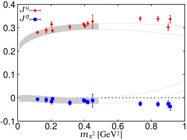
Figure 96: Angular momentum contributions to the nucleon spin (from proceedings [B⁺07g]).

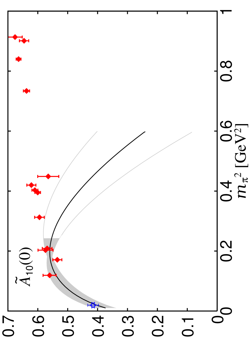
Figure 97: Isosinglet quark spin fraction $\Delta\Sigma^{u+d}$ (from proceedings [B⁺07g]).

We now come back to the unquenched lattice QCD studies of LHPC and QCDSF discussed in the previous section. Figure 97 shows the angular momentum of up- and down quarks, $J^{u,d}=(A^{u,d}_{20}(0)+B^{u,d}_{20}(0))/2$, as a function of $m_{\pi}^{2}$, computed on the basis of the results from QCDSF [B⁺07g] in Figs. 89, 89, 95 and 95, together with the corresponding chiral extrapolations represented by the shaded bands. It is quite remarkable that the total angular momentum (from connected insertions) is mainly carried by the up quarks, while the down quark contribution is very small and tends to zero towards the chiral limit. From the CBChPT extrapolations, the values $J^{u}=0.230(8)$ and $J^{d}=-0.004(8)$ were obtained at the physical pion mass [B⁺07g].

This is in good agreement within errors with the results from LHPC [H⁺08a] based on the simultaneous global chiral fits in Figs. 85 to  87 for the isovector, and Figs. 91 to  93 for the isosinglet channel, giving $J^{u}=0.214(27)$ and $J^{d}=-0.001(27)$.

The total angular momentum contribution from $u+d$ quarks to the spin of the nucleon (obtained from connected diagrams) is therefore $J^{u+d}\approx 40-50\%$ of $1/2$, which is significantly below the values given in Table 1 and obtained in [GJJ02] for the connected contributions, which are of the order $J^{u+d}\approx 80-90\%$ of $1/2$. This discrepancy is certainly to a large extent the result of the different chiral extrapolations, i.e. the linear extrapolation in $m_{\pi}^{2}$ employed in [MDL⁺00] compared to the CBChPT extrapolations used in [B⁺07g] and [H⁺08a]. The band in Fig. 97 shows that a substantial chiral curvature may be expected at smaller pion masses, which cannot be provided by a linear fit to results at larger pion masses.

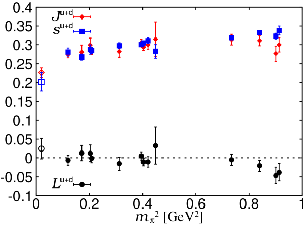
Figure 98: Spin and orbital momentum contributions to the nucleon spin (from proceedings [B⁺07g]).

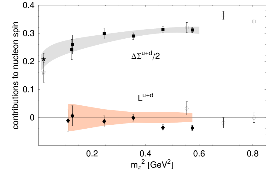
Figure 99: Spin and orbital angular momentum contributions to the nucleon spin (from [H⁺08a]).

An analysis of the quark orbital angular momentum contributions, $L^{q}$, requires, in addition to the total angular momenta $J^{q}$, also the quark spin fractions $\Delta\Sigma^{q}$. For the isovector channel, they were discussed in some detail in section 3.4.4 in terms of the axial vector coupling constant, which we identify with the quark spin fraction, $\Delta\Sigma^{u-d}=\langle 1\rangle_{\Delta u-\Delta d}=g^{u-d}_{A}$. We refer in particular to the results from QCDSF in Fig.36 [K⁺06] and from LPHC in Fig.36 [E⁺06a]. Corresponding results for the spin fraction of quarks in the isosinglet channel, obtained by QCDSF on the basis of the same lattice approach and similar ensembles as discussed before, are displayed in Fig.97 versus $m_{\pi}^{2}$. The shaded band represents a chiral extrapolation based on a leading 1-loop HBChPT calculation [DMS06], which gives

$$\Delta\Sigma^{u+d}=\Delta\Sigma^{0,u+d}\left(1-\frac{3g_{A}^{2}m_{\pi}^{2}}{(4\pi)^{2}f_{\pi}^{2}}\left\{\ln\frac{m_{\pi}^{2}}{\lambda^{2}}+1\right\}\right)+c_{0}m_{\pi}^{2}\,.$$ (156)

A value of $\tilde{A}^{u+d}_{10}(0)=\Delta\Sigma^{u+d}=0.402(24)$ was obtained at the physical pion mass from a fit with two free parameters, $\Delta\Sigma^{0,u+d}$ and $c_{0}$, to the lattice data points with $m_{\pi}<500\text{ MeV}$. The strong downwards bending observed below $m_{\pi}\sim 350\text{ MeV}$ leads to a very good agreement with the recent result from HERMES [A⁺07b], $\Delta\Sigma^{u+d,\exp}=0.415(20)$, represented by the open star. We note, however, that the extrapolation not only breaks down quickly for pion masses above $500\text{ MeV}$, but that leading 1-loop HBChPT is in general not expected to be applicable for pion masses of $300\text{ MeV}$ and larger. The good agreement of the chiral extrapolation with the result from experiment in Fig.97 should therefore be considered with caution and may well be accidental.

Together with the results for $J^{u+d}$ discussed above, the total quark orbital angular momentum contribution was found to be small and compatible with zero within errors, $L^{u+d}=J^{u+d}-\Delta\Sigma^{u+d}/2=0.025(27)$, at the physical pion mass [B⁺07g]. Figure 99 shows that this remarkable cancellation of $J^{u+d}$ and $\Delta\Sigma^{u+d}/2$ also holds over the full range of accessible pion masses up to $m_{\pi}\approx 900\text{ MeV}$.

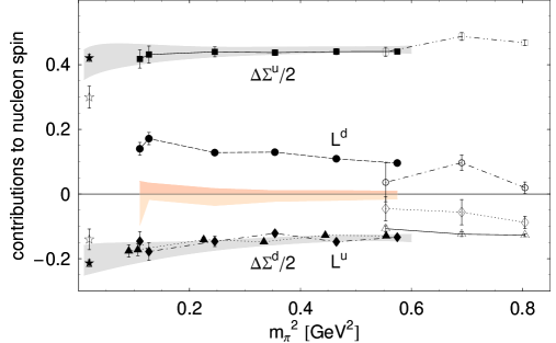
Figure 100: Contributions to the nucleon spin (from [H⁺08a]).

These findings are in good agreement with the results from LHPC [H⁺08a] in Fig. 99, showing the spin and OAM contributions in the isosinglet channel as functions of the squared pion mass. The OAM for $u+d$-quarks, which was in this case obtained from dipole extrapolations of the GFF $B^{u+d}_{20}(t)$ to $t=0$ at fixed pion masses, is also found to be compatible with zero within errors for $m\lesssim 600\text{ MeV}$. The lattice data points for the total quark momentum fraction were extrapolated to the chiral limit based on a self-consistently modified result from leading 1-loop HBChPT,

$$\Delta\Sigma^{u+d}=\Delta\Sigma^{0,u+d}\left(1-\frac{3g_{A,\text{lat}}^{2}}{(4\pi)^{2}}\frac{m_{\pi,\text{lat}}^{2}}{f_{\pi,\text{lat}}^{2}}\left(\ln\frac{m_{\pi,\text{lat}}^{2}}{f_{\pi,\text{lat}}^{2}}+1\right)\right)+c_{0}\frac{m_{\pi,\text{lat}}^{2}}{f_{\pi,\text{lat}}^{2}}\,.$$ (157)

with free parameters $\Delta\Sigma^{0,u+d}$ and $c_{0}$, see also Eq. 148 and corresponding discussion. The chiral fit, which is represented by the error band in Fig. 99, gives $\Delta\Sigma^{u+d}=0.415(56)$, also in very good agreement with recent results by HERMES [A⁺07b].

Together with the results from LHPC for $J^{u,d}$ discussed above, one obtains for the total $u+d$ quark OAM contribution to the nucleon spin a value of $L^{u+d}=J^{u+d}-\Delta\Sigma^{u+d}/2=0.005(52)$ at the physical pion mass [H⁺08a], perfectly consistent with zero and compatible with the results from QCDSF within errors.

Further insight into the nucleon spin structure may be obtained by decomposing the total quark angular momentum into the spin and orbital angular momentum contributions of up- and down-quarks separately. Such a decomposition is displayed in Fig. 100, showing lattice results from LHPC for $\Delta\Sigma^{u,d}$ and $L^{u,d}$ versus $m_{\pi}^{2}$ [H⁺08a]. They were obtained by combining the results for the GFFs $A^{u,d}_{20}(t)$ and $B^{u,d}_{20}(t)$, where the $B^{u,d}_{20}(t)$ were extrapolated to $t=0$ using dipole fits, with the isovector axial vector coupling discussed in section 3.4.4, cf. Fig. 36, providing $\Delta\Sigma^{u-d}$, and for $\Delta\Sigma^{u+d}$ shown in Fig. 99.

The most remarkable feature of this analysis is that the individual up- and down-quark OAM contributions are quite substantial, with absolute values $|L^{u}|\sim|L^{d}|$ of the order of $20-30\%$ of $1/2$, but opposite in sign, so that they cancel almost exactly in the sum, $L^{u+d}\sim 0$. The values at the physical pion mass, obtained from the self-consistently modified HBChPT extrapolation of $\Delta\Sigma^{u+d}$, the SSE extrapolation of $\Delta\Sigma^{u-d}=g_{A}^{u-d}$ [E⁺06a], and the CBChPT extrapolated GFFs $A^{u\pm d}_{20}(t)$ and $B^{u\pm d}_{20}(t)$ are $L^{u}=-0.195(44)$ and $L^{d}=0.200(44)$ [H⁺08a]. Similarly, the individual spin- and OAM contributions of the down-quarks are of the same size, $|L^{d}|\sim|\Delta\Sigma^{d}/2|\sim 0.1,\ldots 0.15$, but also opposite in sign, so that the down-quark angular momentum is zero within errors due to a cancellation of spin and OAM, $J^{d}=L^{d}+\Delta\Sigma^{d}/2\sim 0$.

The observation that the total light quark angular momentum is compatible with zero in lattice QCD, $L^{u+d}\sim 0$, seems at first sight to be at odds with expectations from relativistic quark models, where the quark OAM contribution is in general substantial, $L_{\text{rel}}^{u+d}\sim 30,\ldots,40\%$ of $1/2$. Such a strong discrepancy could in principle point towards significant deficiencies of the model, or substantial systematic effects in the lattice calculation. At the same time, the quark spin contribution $\Delta\Sigma_{\text{rel}}^{u+d}/2$ is approximately $60,\ldots,70\%$ of $1/2$, in overall agreement with lattice results. A likely explanation that can at least partially account for these observations has been given in [WN08, Tho08, B⁺08f] : While the lattice results are given in the $\overline{\text{MS}}$ scheme at a scale of $4\text{ GeV}^{2}$, the model calculations generically correspond to a much lower “hadronic” scale $\mu_{\text{had}}\ll 1\text{ GeV}$, so that the respective numbers may not be compared directly in the first place. At this point it is interesting to note that the evolution equations for spin and OAM in the leading-logarithmic approximation [JTH96], although strictly speaking not applicable at very low scales, predict a strong change in magnitude and even the sign of the quark OAM contributions at scales $\mu^{2}\lessapprox 0.4\text{ GeV}^{2}$. Depending on the initial conditions and the hadronic starting scale, relativistic quark model results were even found to be in rough quantitative agreement with the lattice results when evolved up to the common scale of $4\text{ GeV}^{2}$ [Tho08]. Similarly, the overall consistency between the model and the lattice results for $\Delta\Sigma_{\text{rel}}^{u+d}$ may be understood by noting that the quark spin is conserved at leading-log order.

We note again that many of the lattice results presented in this section correspond to the quark line connected contributions, and that a complete calculation including disconnected diagrams could in principle lead to a significantly different decomposition of the nucleon spin.

A summary of the more recent lattice QCD results for quark spin-, OAM- and total angular momentum contributions to the nucleon spin will be given below in Table 2.

4.4.4 Higher moments of unpolarized and polarized GPDs

4.4.5 Transverse nucleon structure

Higher moments of the unpolarized nucleon GPDs $H$ and $E$ are given by linear combinations of the the GFFs $A_{ni}(t)$, $B_{ni}(t)$ with $n=1,2,3,\ldots$ and $i=0,2,4,\ldots\leq(n-1)$, and $C_{n0}$ with $n=2,4,6,\ldots$, cf. Eqs. (34,35). They coincide with the form factors of the energy momentum tensor for $n=2$ that we discussed in detail in the previous sections. Moments of the polarized GPDs $\widetilde{H}$ and $\widetilde{E}$ are parametrized by the GFFs $\widetilde{A}_{ni}(t)$, $\widetilde{B}_{ni}(t)$ with $n=1,2,3,\ldots$ and $i=0,2,4,\ldots\leq n$ [Häg04].

First results for the $n=2$ moments of the polarized GPDs were presented in [S⁺04] in unquenched lattice QCD. The unpolarized and polarized moments with $n=1,2,3$ and $i=0$ have been investigated for the first time by LHPC/SESAM in [H⁺04] for $n_{f}=2$ flavors of Wilson fermions in a “heavy pion world” with pion masses of $\approx 744\text{ MeV}$ and $\approx 897\text{ MeV}$. In this study, the focus has been on the change of the $t$-dependence (the slope) of the GFFs $A^{q}_{n0}(t)$ and $\widetilde{A}^{q}_{n0}(t)$ when going from the lowest moment $n=1$ (the form factors) to the highest accessible moment, $n=3$. The physics behind these results will be discussed below. Since then, a number of results, mostly for $A^{q}_{n0}(t)$, $B^{q}_{n0}(t)$, $\widetilde{A}^{q}_{n0}(t)$ and $\widetilde{B}^{q}_{n0}(t)$ for the lowest $n$, obtained in unquenched QCD, were presented in proceedings, see, e.g., [G⁺05c, G⁺06a, G⁺05b, G⁺07c, B⁺07g, S⁺04, N⁺04, E⁺06b, B⁺08f]. The most comprehensive lattice study to this date of moments of unpolarized and polarized GPDs for $n=1,2,3$ and $i=0$ was published more recently by LHPC, in the framework of the hybrid approach with $n_{f}=2+1$ flavors of domain wall valence and Asqtad staggered sea quarks [H⁺08a]. For a discussion of the corresponding results for the unpolarized $n=2$-moments, we refer to section 4.4.2, cf. Figs. 83, 85 to 87, and 91 to 93.

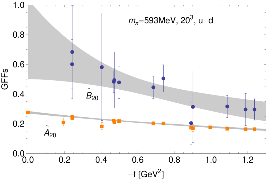
Figure 101: The GFFs $\widetilde{A}^{u-d}_{20}(t)$ and $\widetilde{B}^{u-d}_{20}(t)$ at a pion mass of $595\text{ MeV}$ (from [H⁺08a]).

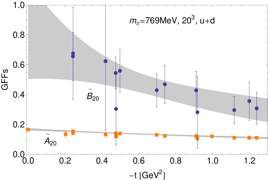
Figure 102: Connected contributions to the GFFs $\widetilde{A}^{u+d}_{20}(t)$ and $\widetilde{B}^{u+d}_{20}(t)$ at a pion mass of $758\text{ MeV}$ (from [H⁺08a]).

An example for the polarized GFFs $\widetilde{A}_{20}(t)$ and $\widetilde{B}_{20}(t)$ is given in Figs. 102 and 102 for the isovector channel at a pion mass of $\approx 595\text{ MeV}$, and for the isosinglet channel at a pion mass of $\approx 758\text{ MeV}$, respectively. As for the unpolarized case, the underlying axial vector lattice operators were perturbatively renormalized including a non-perturbative improvement factor as given in Eq. 140, and all results are given in the $\overline{\text{MS}}$ scheme at a scale of $\mu=2\text{ GeV}$. While the statistical precision for the GFF $\widetilde{A}_{20}(t)$ is very good, the signal for $\widetilde{B}^{u+d}_{20}(t)$ in particular is rather noisy with errors of $\mathcal{O}(50\%)$ and larger at pion masses of $\approx 595\text{ MeV}$ and below. Still, within errors the GFF $\widetilde{B}_{20}(t)$ turns out to be large compared to $\widetilde{A}_{20}(t)$, with central values of $\widetilde{B}^{u-d}_{20}(t)\sim\widetilde{B}^{u+d}_{20}(t)\sim 0.6$ at the lowest accessible values of $-t\simeq 0.25\text{ GeV}^{2}$. We note that in particular the pion mass dependence of the forward values $\langle x\rangle_{\Delta u-\Delta d}=\widetilde{A}^{u-d}_{20}(t\text{{=}}0)$ (obtained in this lattice simulation framework) was presented and discussed in section 4.3.2, Fig 78. Further results for $\widetilde{A}_{20}(t)$ and $\widetilde{B}_{20}(t)$ for pion masses down to $\approx 350\text{ MeV}$ can be found in [H⁺08a].

A direct comparison of the $t$-dependences of the lowest three moments of the unpolarized GPD $H$, $A_{(n=1,2,3)0}(t)$, in the isovector and isosinglet channel is provided in Figs. 104 and 104 for $m_{\pi}\approx 496\text{ MeV}$, where the GFFs have been normalized to unity at $t=0$. Dipole fits with fixed forward values, $A_{(n=1,2,3)0}(t\text{{=}}0)=1$, to the lattice data points are represented by the shaded bands. In both the isovector and isosinglet case, the slope in $t$ is found to flatten significantly for increasing $n$, confirming the results of the first unquenched lattice QCD study by LHPC/SESAM [H⁺04] of $A^{u\pm d}_{n0}(t)$ and $\widetilde{A}^{u-d}_{n0}(t)$ at larger pion masses.

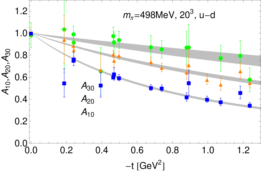
Figure 103: Lowest three moments of the unpolarized GPD $H(x,\xi=0,t)$ for $u-d$ (from [H⁺08a]).

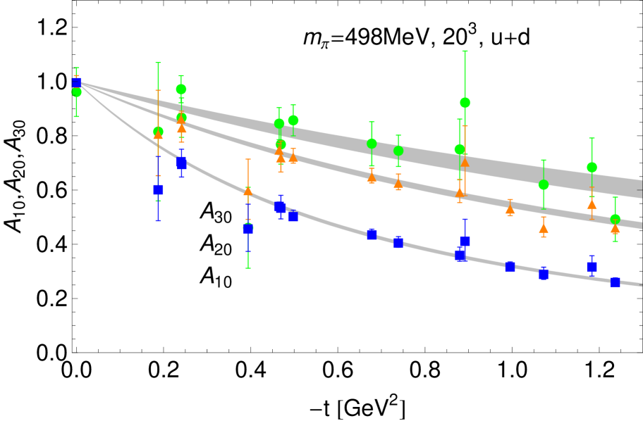
Figure 104: Lowest three moments of the unpolarized GPD $H(x,\xi=0,t)$ for $u+d$ (from [H⁺08a]). Contributions from disconnected diagrams are not included.

An simple interpretation of this interesting observation can be given in the framework of the light-cone wave function (LCWF) or overlap representations of the GPDs in [BDH01, DFJK01]). There, one finds that the dependence of the LCWF of the outgoing hadron on the quark transverse momentum, upon interaction with an external current, is given by $k^{\text{LCWF}}_{f,\perp}=k^{\text{LCWF}}_{i,\perp}-(1-x)\Delta_{\perp}$, where $x$ is the longitudinal momentum fraction carried by the active quark, $k^{\text{LCWF}}_{i,\perp}$ is the initial transverse momentum in the LCWF, and $\Delta_{\perp}\sim|t|^{1/2}$ is the transferred transverse momentum (in the frame specified in [BDH01]). Hence at small $x$, the intrinsic transverse momentum dependence of the LCWF changes strongly for larger values of the momentum transfer $\Delta_{\perp}$, leading to a small wavefunction overlap. Physically, the large transferred momentum would have to be redistributed among all constituents to prevent a break-up of the bound state. As a result, the coupling to the external current, parametrized by the GPDs, is suppressed. For $x\rightarrow 1$, $k^{\text{LCWF}}_{f,\perp}\sim k^{\text{LCWF}}_{i,\perp}$, the wavefunction overlap is large, corresponding to a higher probability that the hadron stays intact, even for larger $\Delta_{\perp}^{2}=-t^{2}$. In this case, a stronger coupling to the hadron will be observed. Concerning moments of PDFs and GPDs, we note that the limit $n\rightarrow\infty$ corresponds to $x\rightarrow 1$ due to the weighting with high powers $x^{n-1}$, Eq. (4). From the above discussion, we therefore expect that the (relative) coupling to the hadron at larger $t$, as parametrized by the generalized form factors, increases for increasing $n$. More precisely, it is predicted that the GFFs approach a constant in $t$ for infinitely high moments,

$$\frac{A_{n0}(t)}{A_{n0}(t\text{{=}}0)}\xrightarrow{n\rightarrow\infty}1\;.$$ (158)

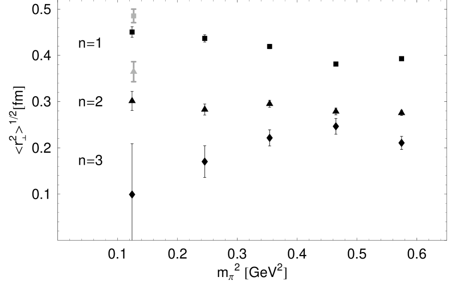
Figure 105: Isovector (generalized) transverse charge radii for $n=1,2,3$ (from [H⁺08a]).

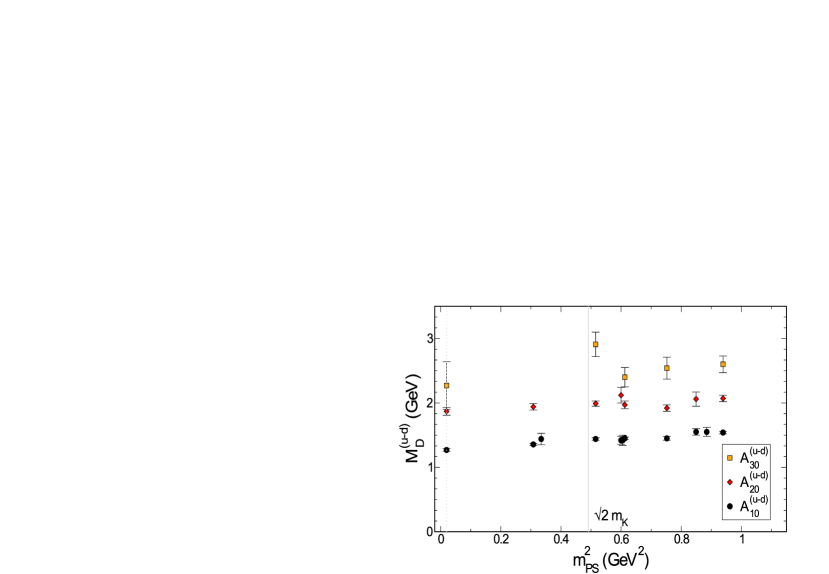
Figure 106: Dipole masses of the GFFs $A^{u-d}_{n0}$ for $n=1,2,3$ (from proceedings [G⁺05b]).

This is qualitatively confirmed in Fig. 104, which shows that the relative coupling for $n=3$ is already a remarkable factor of 2 larger than the coupling for $n=1$, i.e. $A^{u-d}_{30}(t)/A^{u-d}_{30}(0)\sim 2A^{u-d}_{10}(t)/A^{u-d}_{10}(0)$ for, e.g., a squared momentum transfer of $-t\approx 1\text{ GeV}^{2}$, at the given pion mass. The effect is also clearly visible but less pronounced for the polarized case [H⁺04, H⁺08a].

An analogous and possibly even more intuitive interpretation of these observations may be given in impact parameter (transverse coordinate) space [Bur00]. The impact parameter dependent GPDs (and GFFs) are obtained by Fourier-transforming the momentum space GPDs (GFFs) with respect to the transverse momentum transfer, $t=-\Delta_{\perp}^{2}$, as given in Eq. 64, for $\xi=0$. The impact parameter, $b_{\perp}$, specifies the distance of the active quark to the center of momentum (COM) of the parent hadron, $R_{\perp}=\sum_{i}x_{i}r_{i,\perp}/\sum_{i}x_{i}=\sum_{i}x_{i}r_{i,\perp}$ where the sums run over all partons. In the limit $x\rightarrow 1$, the active parton carries all the momentum and therefore represents the COM. Hence it is expected that the impact parameter distribution of partons peaks around $b_{\perp}=0$ as $x$ approaches unity. Formally, using, e.g., light cone hadron wave functions, it can be shown that the GPD $H(x,\xi=0,t)$, transformed to impact parameter space, is proportional to a delta function in the limit $x\rightarrow 1$, $q(x,b_{\perp})=H(x,b_{\perp})\overset{x\rightarrow 1}{\propto}\delta^{2}(b_{\perp})$ [Die02]. This is of course in one-to-one correspondence with the prediction of the $t$-independence of the GFFs in momentum space as $n\rightarrow\infty$, cf. Eq. (158).

A measure of the transverse size of a hadron is given by the (generalized) transverse mean squared radius [H⁺04],

$$\langle r_{\perp}^{2}\rangle_{n}=\frac{\int d^{2}b_{\perp}b^{2}_{\perp}\int dxx^{n-1}q(x,\vec{b}_{\perp})}{\int d^{2}b_{\perp}\int dxx^{n-1}q(x,\vec{b}_{\perp})}=\frac{\int d^{2}b_{\perp}b^{2}_{\perp}A_{n0}(b_{\perp})}{\int d^{2}b_{\perp}A_{n0}(b_{\perp})}\,,$$ (159)

which coincides with the standard (transverse) mean square charge radius for $n=1$, $\langle r_{\perp}^{2}\rangle_{n=1}=\langle r_{\perp}^{2}\rangle=\frac{2}{3}\langle r^{2}\rangle$, defined through the Dirac form factor $F_{1}(Q^{2})=A_{10}(t)$ as in Eq. (60). From what has been said above, the transverse size of the hadron as measured by $\langle r_{\perp}^{2}\rangle_{n}$ is expected to vanish in the limit $n\rightarrow\infty$. We also note that the generalized mean square charge radii are directly related to dipole masses, $\langle r_{\perp}^{2}\rangle_{n}=8/m^{2}_{D,n}$, obtained from, e.g., dipole fits to the lattice data for the GFFs $A_{(n=1,2,3)0}(t)$, as represented by the bands in Figs. 104 and 104. Figure 106 shows the pion mass dependence of isovector transverse RMS radii $\langle r_{\perp}^{2}\rangle^{1/2}_{n}$ for $n=1,2,3$, obtained by LHPC from dipole fits to the lattice data for $|t|\lessapprox 1\text{ GeV}^{2}$ [H⁺08a]. As the pion mass decreases, the significant spread between $\langle r_{\perp}^{2}\rangle^{1/2}_{n=1}$ and $\langle r_{\perp}^{2}\rangle^{1/2}_{n=3}$ seems to increase. However, the statistical errors are quite large at the lowest pion mass, and the data points in Fig. 106 are in addition subject to systematic uncertainties related to the dipole ansatz used to parametrize the GFFs, as well as the region of $t$ included in the dipole fits. More precise lattice results are needed before fully quantitative predictions about the decrease of the transverse size of the nucleon for increasing $x$ at the physical pion mass can be made.

Corresponding results for the generalized axial-vector charge radii also show a decrease from $n=1$ to $n=3$ [H⁺08a], which is however not as pronounced as for the vector case in Fig. 106.

Similar conclusions about the decrease of the nucleon transverse size were reached independently by QCDSF based on simulations with $n_{f}=2$ flavors of clover-improved Wilson fermions, see, e.g., [G⁺05b]. A summary of the results is displayed in Fig. 106, showing the dipole masses $m_{D}^{u-d}$, obtained from fits to the lattice data for the GFFs $A^{u-d}_{(n=1,2,3)0}(t)$, as functions of $m_{\pi}^{2}$. As before, a significant increase of the dipole masses is observed, going from $n=1$ to $n=3$. We note that the results in Fig. 106 for $n=1$ correspond to the results for the Dirac radii shown in Fig. 20.

As we have discussed in section 3.4.2, the lattice QCD results for the Dirac radius lie approximately a factor of two below the value from experiment at the lowest accessible pion masses. We therefore would like to stress that a proper chiral extrapolation of the lattice data points in Fig. 106 and also in Fig. 106 will be, at least for $n=1$, highly non-linear and may lead to significantly different conclusions about the transverse nucleon structure at the physical pion mass.

4.4.6 Tensor GPDs and the transverse spin structure of hadrons

Having discussed lattice QCD results for moments of unpolarized and polarized (vector and axial-vector) GPDs, we now turn our attention to the tensor (also quark helicity flip or transversity) GPDs of the pion, $H^{\pi}_{T}(x,\xi,t)$ (Eq. 9), and the nucleon, $H_{T}(x,\xi,t)$, $E_{T}(x,\xi,t)$, $\widetilde{H}_{T}(x,\xi,t)$ and $\widetilde{E}_{T}(x,\xi,t)$ (Eq. 16). The corresponding $x^{n-1}$-moments are parametrized by the the GFF $B^{\pi}_{Tni}(t)$ for the pion, see Eqs. (9,11), and the tensor GFFs $A_{Tni}(t)$, $\overline{B}_{Tni}(t)$, $\widetilde{A}_{Tni}(t)$ and $\widetilde{B}_{Tn(i+1)}(t)$ for the nucleon, with $n=1,2,3,\ldots$ and $i=0,2,4,\ldots\leq(n-1)$, and where $\widetilde{B}_{T11}(t)=0$ due to time reversal symmetry constraints, see Eqs. (22,29) [Häg04].

4.4.7 Pion

In this section, we present first lattice QCD results for the pion tensor form factor $B^{\pi}_{T10}(t=-Q^{2})$ as defined in Eq. 9 and the corresponding next highest moment, $B^{\pi}_{T20}(t=-Q^{2})$, Eq. (11). Based on the same set of $n_{f}=2$ improved Wilson fermion and Wilson gauge action ensembles that were used for the study of the pion form factor discussed in section 3.3, Figs. 10 and 10, QCDSF/UKQCD recently computed $B^{\pi}_{Tn0}(t)$ for $n=1,2$ in a range of $-t\approx 0.3,\ldots,3\text{ GeV}^{2}$ [B⁺08h]. The underlying local tensor operators have been non-perturbatively renormalized, and the results were transformed to the $\overline{\text{MS}}$ scheme at a scale of $4\text{ GeV}^{2}$. A typical result for the $t$-dependence of the pion tensor form factor $B^{\pi}_{T10}(t)$ and the GFF $B^{\pi}_{T20}(t)$ is shown in Fig. 108 for a pion mass of $\approx 600\text{ MeV}$. Using a $p$-pole ansatz of the form

$$F(t)=\frac{F(0)}{\left(1-\frac{t}{p\,m_{p}^{2}}\right)^{p}}\,,$$ (160)

with free parameters $F(0)$ and $m_{p}^{2}$, the results for $B^{\pi}_{Tn0}(t)$ have been fitted and extrapolated to $t=0$. Since the pion tensor GFFs $B^{\pi}_{Tn0}(t)$ are defined (see, e.g., Eq. 9) including a normalization factor of $1/m_{\pi}$, they have to be proportional to $m_{\pi}$, and therefore vanish in the chiral limit, as predicted by ChPT [DMS07]. It is therefore sensible to study the chiral extrapolations of $B^{\pi}_{Tn0}(t\text{{=}}0)/m_{\pi}$, which are presented in Fig. 108 as functions of $m_{\pi}^{2}$, obtained for $p=1.6$. The lattice results are, for the accessible pion masses from $\approx 400$ to $\approx 1000\text{ MeV}$, within errors well compatible with a linear dependence on $m_{\pi}^{2}$. In order to account for uncertainties due to possible finite volume effects, an ansatz of the form $B^{\pi}_{Tn0}(t\text{{=}}0)/m_{\pi}=c_{0}+c_{1}m_{\pi}^{2}+c_{2}m_{\pi}^{2}\exp(-m_{\pi}L)$, where $L$ is the spatial lattice extent, with free parameters $c_{i}$, has been used to fit the lattice data points separately for $n=1,2$ and extrapolate to the physical point. This fit is represented by the dark shaded band in Fig. 108.

Although predictions from 1-loop ChPT [DMS07] are strictly speaking not applicable at the accessible pion masses and volumes, they still might give a qualitative idea about the uncertainties related to the chiral extrapolation. To this extent, additional fits based on 1-loop ChPT,

$$\hat{B}^{\pi}_{Tn0}(t\text{{=}}0,m_{\pi}) = \hat{B}^{\pi,0}_{Tn0}\left(1+c_{1}^{(n)}\frac{m_{\pi}^{2}}{(4\pi)^{2}f_{\pi}^{2}}\left\{\ln\frac{m_{\pi}^{2}}{\lambda^{2}}+1\right\}\right)+c_{2}^{(n)}m_{\pi}^{2}+c_{3}^{(n)}m_{\pi}^{2}e^{-m_{\pi}L}\,,$$ (161)

with chiral coefficients $c_{1}^{(1)}=1/2$, $c_{1}^{(2)}=-3/2$, and where $\hat{B}^{\pi}_{Tn0}=B^{\pi}_{Tn0}/m_{\pi}$ and $\hat{B}^{\pi,0}_{Tn0}=\hat{B}^{\pi}_{Tn0}(m_{\pi}\text{{=}}0)$, including finite volume correction terms $c_{3}^{(n)}m_{\pi}^{2}\exp(-m_{\pi}L)$ that were added by hand, have been performed to the lattice data points for $m_{\pi}<650\text{ MeV}$.

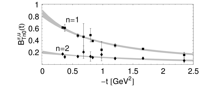
Figure 107: Tensor (generalized) form factors $B^{\pi}_{Tn0}(t)$ for up-quarks in a $\pi^{+}$ with $m_{\pi}\sim 600\text{ MeV}$ (from [B⁺08h]).

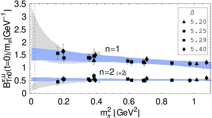
Figure 108: Forward values of tensor (generalized) form factors for up-quarks in a $\pi^{+}$ as a function of the pion mass squared (from [B⁺08h]).

The results are represented by the lighter shaded band in Fig. 108. From the linear chiral extrapolation in Fig. 108, already a rather large value of $B^{\pi}_{T10}(t\text{{=}}0)/m_{\pi}=1.54(24)\text{ GeV}^{-1}$ was found at the physical point, while the extrapolation based on 1-loop ChPT tends to give an even larger central value. Analogously to the case nucleon tensor GFF $\overline{B}_{T10}$ introduced in section 2.1.1, one may define a tensor anomalous magnetic moment of the pion, $\kappa_{T}^{\pi}=B^{\pi}_{T10}(t\text{{=}}0)$, for which a value of $\kappa_{T}^{\pi}=0.215(33)$ is obtained at the physical pion mass from the linear chiral extrapolation in Fig. 108. Also based on a linear chiral extrapolation in $m_{\pi}^{2}$, a value of $m_{p}=0.756(95)\text{ GeV}$ was obtained for the corresponding $p$-pole mass at the physical point, with $p=1.6$.

In the case of $B^{\pi}_{T20}(t\text{{=}}0)$, the result of the linear extrapolation (represented by the dark shaded band), is $B^{\pi}_{T20}(0)/m_{\pi}=0.277(71)\text{ GeV}^{-1}$ at the physical pion mass and the infinite volume limit. A value of $m_{p}=1.130(265)\text{ GeV}$ was found for the corresponding $p$-pole mass with $p=1.6$, obtained from a linear chiral extrapolation in $m_{\pi}^{2}$ to the physical pion mass. The fit based on 1-loop ChPT, Eq. 161, shown by the light shaded band in Fig. 108, clearly gives a much smaller value for $B^{\pi}_{T20}(t\text{{=}}0)$ at the physical point, nearly compatible with zero within errors. We note again, however, that the results from a 1-loop ChPT fit at such large pion masses cannot be regarded as reliable, and only provide an indication for uncertainties in the chiral extrapolation.

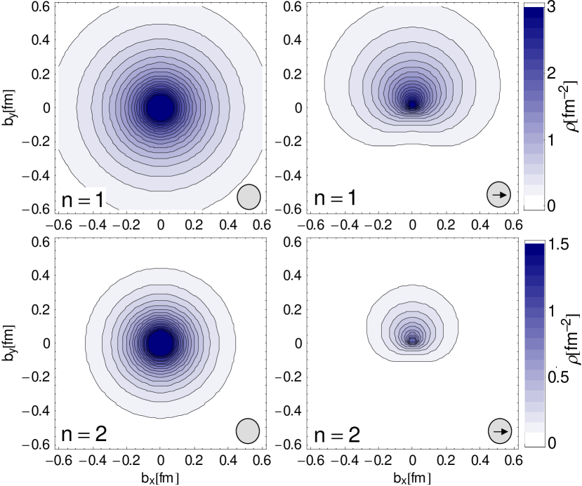
Figure 109: Density of transversely polarized up-quarks in the $\pi^{+}$ (from [B⁺08h]).

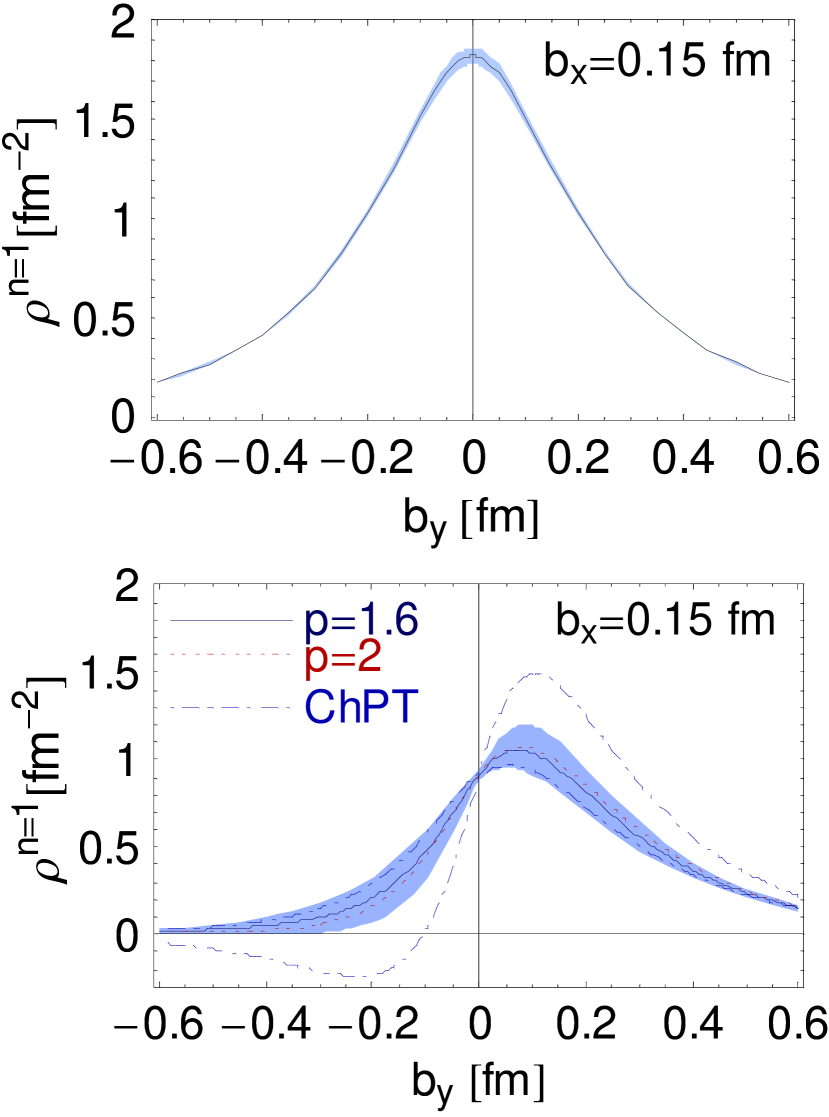
Figure 110: Density profiles for transversely polarized up-quarks in the $\pi^{+}$ (from [B⁺08h]).

As we will explain in the following, the lattice results for the moments of the pion vector and tensor GPDs may be used for a first study of the spin structure of the pion.

It has been noted in [B⁺08h] that the $x^{n-1}$-moments of the density of transversely polarized quark with transverse spin $s_{\perp}$ in a pion is given by

$$\rho^{n}(b_{\perp},s_{\perp})=\int_{-1}^{1}dx\,x^{n-1}\rho(x,b_{\perp},s_{\perp})=\frac{1}{2}\left(\mskip 1.5muA^{\pi}_{n0}(b_{\perp}^{2})-\frac{s_{\perp}^{i}\epsilon^{ij}\mskip 1.5mub_{\perp}^{j}}{m_{\pi}}\,\frac{\partial}{\partial b_{\perp}^{2}}\,B_{Tn0}^{\pi}(b_{\perp}^{2})\,\right)\,,$$ (162)

where the GFFs $A^{\pi}_{n0}(b_{\perp}^{2})$ and $B_{Tn0}^{\pi}(b_{\perp}^{2})$ in impact parameter space are related to the momentum-space GFFs $A^{\pi}_{n0}(t)$ and $B_{Tn0}^{\pi}(t)$ by a Fourier-transformation as in Eq. (64). A numerical evaluation of the density $\rho^{n}(b_{\perp},s_{\perp})$ using the lattice results requires representations of the GFFs as functions of $b_{\perp}$. To this end, the $p$-pole parametrization in Eq. (160) was Fourier-transformed to impact parameter space and used together with the numerical lattice results for the forward values, $F(0)$, and the respective $p$-pole masses, $m_{p}$, obtained from $p$-pole fits to the lattice data points and subsequent chiral extrapolations to the physical pion mass. For the pion form factor $A^{\pi}_{10}(t)=F_{\pi}(t)$, the results from [B⁺07f], discussed in section 3.3, Figs 10 and 10, were used, giving a monopole mass of $m_{\text{mono}}=0.727\pm 0.054_{\text{stat+vol+sys}}\text{ GeV}$, in addition to the renormalization condition $F_{\pi}(t\text{{=}}0)=1$ as required by charge conservation. The lattice results for the GFF $A_{20}^{\pi}(t)$ were also parametrized using a monopole ($p=1$) ansatz, with a forward value of $A_{20}^{\pi}(t\text{{=}}0)\approx 0.26$ and a monopole mass of $m_{\text{mono}}\approx 1.2\text{ GeV}$ [B⁺06e]. For the GFFs $B_{Tn0}^{\pi}$, the results of the linear chiral extrapolations of $B_{Tn0}^{\pi}(t=0)/m_{\pi}$ and the corresponding $p$-pole masses, presented above, were employed [B⁺07h, B⁺08h].

Figure 110 shows the final results for the $n=1$ (upper part of figure) and $n=2$ (lower part of figure) moments of the density of up-quarks in a $\pi^{+}$. In contrast to the unpolarized, symmetric densities on the left, the densities for up-quarks with transverse spin in the $x$-direction, $s_{\perp}=(1,0)$, on the right in Fig. 110 are significantly deformed due to the dipole-terms $\propto s_{\perp}^{i}\epsilon^{ij}b_{\perp}^{j}{\partial}_{b_{\perp}^{2}}B_{Tn0}^{\pi}(b_{\perp}^{2})$ in Eq. 162 in combination with the large non-zero values that were found in particular for the tensor GFFs $B_{Tn0}^{\pi}$.

In order to see how the various statistical and systematic uncertainties of the analysis affect the deformation, Fig. 110 shows profile plots of the $n=1$-densities for $b_{x}=0.15\text{ fm}$ as functions of $b_{y}$. While the shaded bands represent the statistical uncertainties from the linear chiral extrapolations in $m_{\pi}^{2}$, the dash dotted lines represent the results for the minimal and maximal values obtained for $B_{T10}^{\pi}(t=0)$ from the 1-loop ChPT extrapolation based on Eq. 161 and displayed in Fig. 108. Even for the smallest values of $B_{T10}^{\pi}(t=0)$, there is still a deformation visible. On the other hand, for the maximal values the density becomes negative for $b_{y}\lessapprox-0.1\text{ fm}$, which is unphysical. This demonstrates that 1-loop ChPT applied to pion masses of $m_{\geq}400\text{ MeV}$ is quantitatively unreliable and in the best case only gives a rough idea about the trend of the chiral extrapolation.

In summary, the large values obtained by QCDSF [B⁺08h] in particular for the tensor anomalous magnetic moment of the pion, $k^{\pi}_{T}=B_{T10}^{\pi}(t\text{{=}}0)$, as displayed in Fig. 108, point towards a surprisingly non-trivial transverse spin structure of the pion, as demonstrated by the deformed densities in Fig. 110.

Clearly, more precise data from lattice QCD at lower pion masses and in larger volumes, together with improved results from ChPT, are required before quantitative predictions can be made for the densities at the physical point.

For a discussion of a possible relevance of these lattice results for the transverse momentum dependent Boer-Mulders function $h_{1}^{\perp,\pi}(x,k_{\perp})$ for pions and azimuthal asymmetries in semi-inclusive deep inelastic scattering and Drell-Yan production, we refer to [B⁺08h] and references therein.

4.4.8 Nucleon

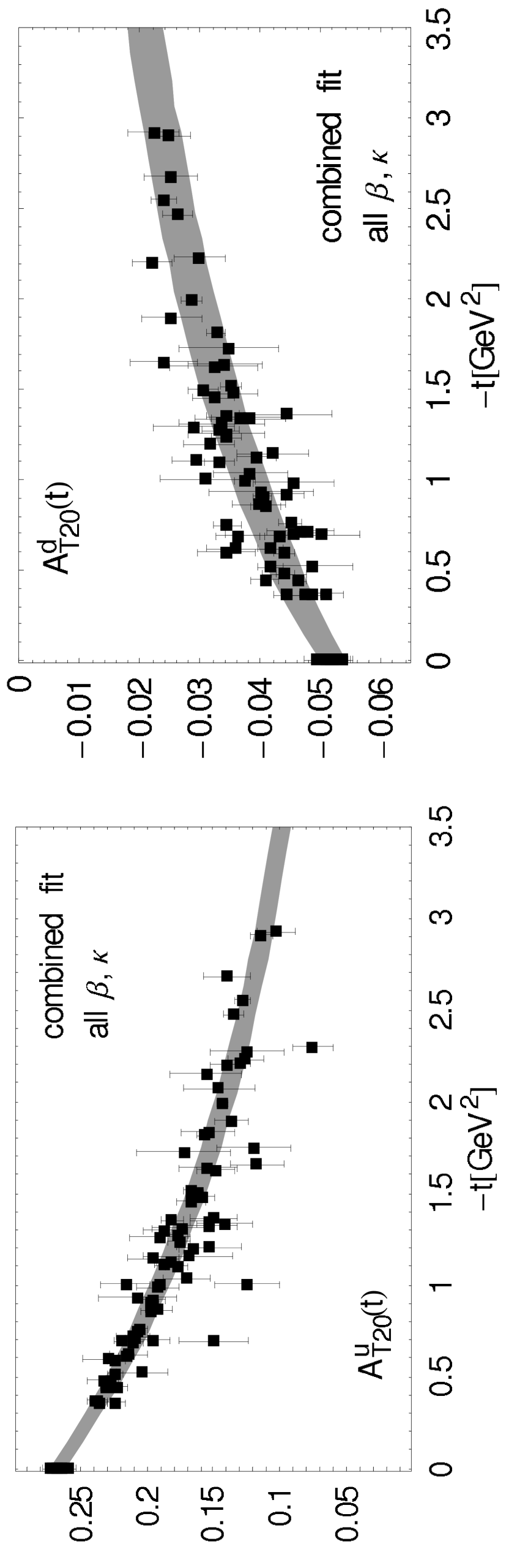
Figure 111: Tensor form factor $A_{T20}(t)$ (from [G⁺05g]).

In the same framework of simulations with $n_{f}=2$ flavors of clover-improved Wilson fermions, QCDSF/UKQCD has also performed calculations of the tensor GFFs of the nucleon [G⁺05g]. The relevant lattice tensor operators have been non-perturbatively renormalized, and all results were transformed to the $\overline{\text{MS}}$ scheme at a scale of $\mu^{2}=4\text{ GeV}^{4}$. An overview of the up- and down-quark contributions to the GFF $A_{T20}(t)$ is given in Fig. 111, based on the same lattice parameters and ensembles as discussed in relation with the corresponding results for $A_{T10}(t)$ in Fig. 39. Using a generalized dipole ansatz of the form Eq. 139, a simultaneous global fit to the full $t$-, $m_{\pi}$- and $a$-dependence of the lattice results was performed, including all available ensembles. Based on the fit, the lattice data points were shifted to $a=0$ and $m_{\pi}=140\text{ MeV}$, and the result is given in Fig. 111. We note that the forward values for $A^{q}_{T20}(t\text{{=}}0)=\langle x\rangle_{\delta q}$ obtained in the framework of this analysis have already been presented above at the end of section 4.3.2, Fig. 81. From the simultaneous global fit, represented by the error band in Fig. 111, the values $A^{u}_{T20}(t=0)=\langle x\rangle_{\delta u}=0.268(6)$ with $m^{u}_{D}=2.31(7)\text{ GeV}$ and $A^{d}_{T20}(t=0)=\langle x\rangle_{\delta d}=-0.052(2)$ with $m^{d}_{D}=2.45(17)\text{ GeV}$ were found at the physical point.

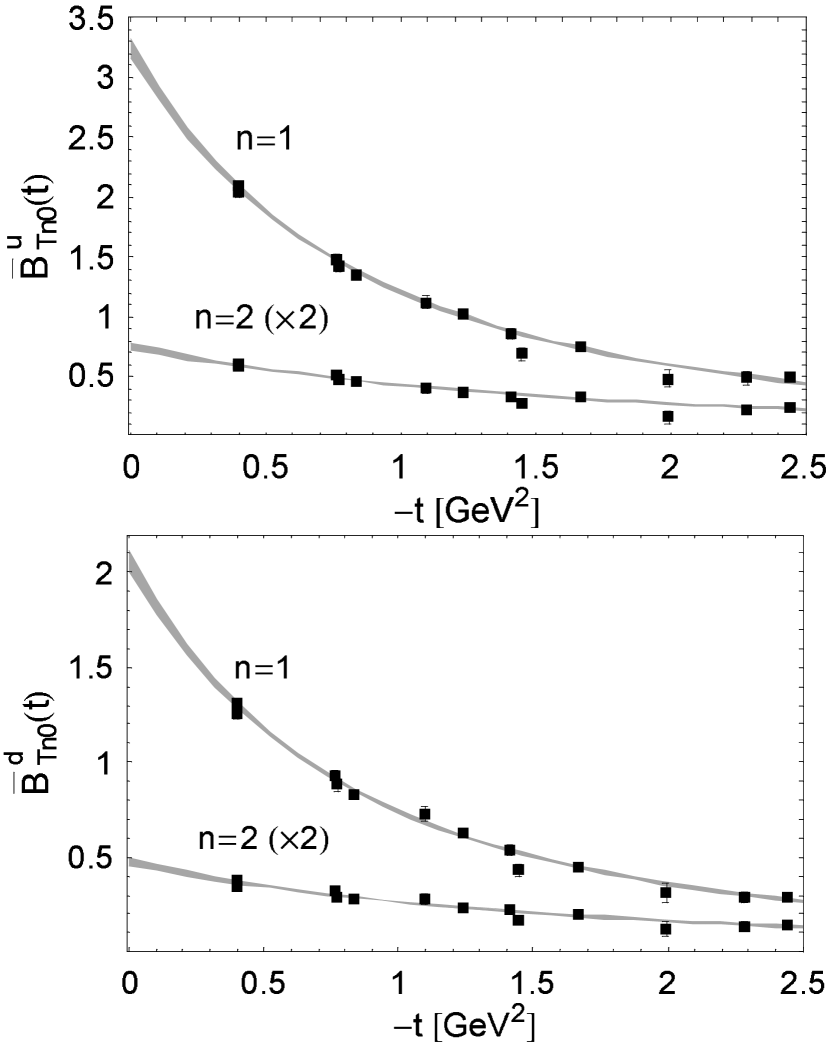
Figure 112: Tensor form factor $\overline{B}_{T10}(t=Q^{2})$ (from [G⁺07d]).

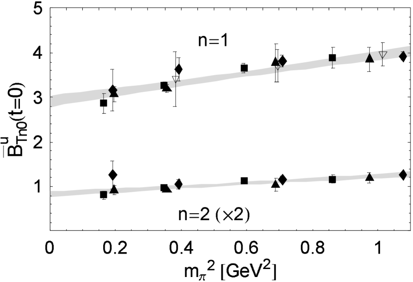
Figure 113: Pion mass dependence of the form factor $\overline{B}_{T10}(Q^{2}=0)$ (from [G⁺07d]).

First results for the nucleon tensor form factor $\overline{B}_{T10}(t=-Q^{2})$, Eq. 22, and the GFF $\overline{B}_{T20}(t)$, Eq. 29, in the same lattice framework as before, i.e. for simulations with $n_{f}=2$ flavors of clover-improved Wilson fermions, were presented by the QCDSF-UKQCD collaboration in [G⁺07d]. Examples for the $t$-dependences of the tensor form factor $\overline{B}_{T10}(t)$ and the GFF $\overline{B}_{T20}(t)$ for up- and down-quarks are presented in Fig. 113 for a pion mass of $\approx 600\text{ MeV}$ and a coupling of $\beta=5.29$ [G⁺07d], showing a quite remarkable statistical precision. The lattice data points for $\overline{B}_{Tn0}(t)$ were fitted with a $p$-pole ansatz, Eq. 160, with $p=2.5$, as given by the shaded bands, and extrapolated to $t=0$. Interestingly, the extrapolated forward values $\overline{B}_{Tn0}(t\text{{=}}0)$ drop substantially going from $n=1$ to $n=2$, with a ratio of $\overline{B}_{T20}(t\text{{=}}0)/\overline{B}_{T10}(t\text{{=}}0)\approx 0.12$ for both flavors.

Figure 113 shows the pion mass dependence of the $\overline{B}^{u}_{Tn0}(t=0)$, together with linear extrapolations in $m_{\pi}^{2}$ to the chiral limit represented by the error bands. At this point we note that the pion mass dependent nucleon mass $m_{N}(m_{\pi})$ has been used in the extraction of $\overline{B}_{Tn0}$ based on the parametrization in Eq. 22, which clearly influences the slope in $m_{\pi}^{2}$ in Fig. 113. Although results from HBChPT to leading 1-loop order for the pion mass and $t$-dependence of the tensor GFFs are available [DMS06, DMS07, ACK06], they are most likely not applicable at the accessible pion masses of $\approx 400\text{ MeV}$ and larger, and were therefore not utilized for the chiral extrapolation of the lattice data.

Concerning the form factor $\overline{B}_{T10}$, it has been suggested [Bur05] to identify its forward value with a tensor anomalous magnetic moment, $\kappa_{T}=\overline{B}_{T10}(t\text{{=}}0)$, in analogy to the standard nucleon anomalous magnetic moment $\kappa=F_{2}(t\text{{=}}0)$. The linear chiral extrapolation in $m_{\pi}^{2}$, represented by the shaded band in Fig. 113, gives for up-quarks $\kappa^{u}_{T}=2.93(13)$ and for down-quarks $\kappa^{d}_{T}=1.90(9)$. These values, which may be compared to the up- and down quark contributions to the anomalous magnetic moments, $\kappa^{u}_{\text{exp}}\approx 1.67$ and $\kappa^{d}_{\text{exp}}\approx-2.03$, are remarkably large and, in contrast to $\kappa^{u,d}$, also of the same sign. In the case of the GFF $\overline{B}_{T20}$, the linear extrapolation of the forward values to the physical pion mass gives $\overline{B}^{u}_{T20}(t=0)=0.420(31)$ and $\overline{B}^{d}_{T20}(t=0)=0.260(23)$.

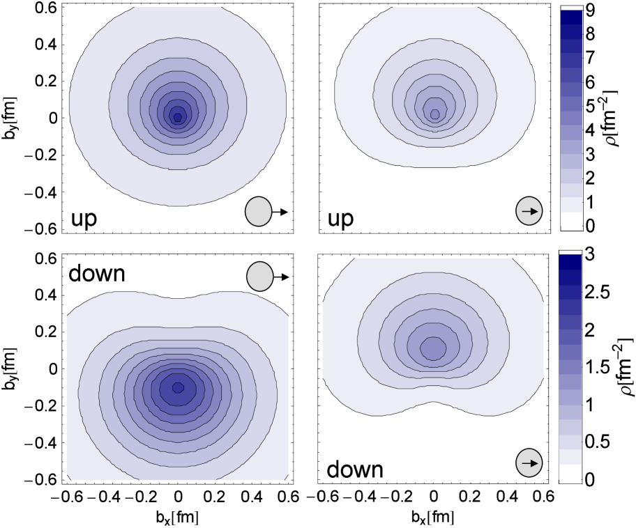
Figure 114: Transverse spin densities of quarks in the nucleon for $n=1$ (from [G⁺07d]).

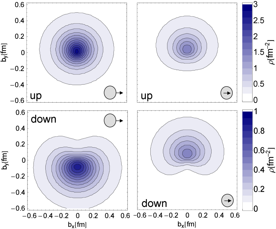
Figure 115: Transverse spin densities of quarks in the nucleon for $n=2$ (from [G⁺07d]).

The tensor generalized form factors in particular provide important information about the nucleon transverse spin structure. To see this more clearly, we note that the $x^{n-1}$-moments of the spin density of transversely polarized quarks in the nucleon [DH05], Eq. 65, are given by

$$\rho^{n}(b_{\perp},s_{\perp},S_{\perp}) = \int_{-1}^{1}dx\,x^{n-1}\rho(x,b_{\perp},s_{\perp},S_{\perp})$$ (163)

$$= \frac{1}{2}\left\{A_{n0}(b_{\perp}^{2})+s_{\perp}^{i}S_{\perp}^{i}\left(A_{Tn0}(b_{\perp}^{2})-\frac{1}{4m_{N}^{2}}\Delta_{b_{\perp}}\widetilde{A}_{Tn0}(b_{\perp}^{2})\right)\right.$$

$$+ \frac{b_{\perp}^{j}\epsilon^{ji}}{m_{N}}\left(S_{\perp}^{i}B_{n0}^{\prime}(b_{\perp}^{2})+s_{\perp}^{i}\overline{B}_{Tn0}^{\prime}(b_{\perp}^{2})\right)$$

$$+ \left.s_{\perp}^{i}(2b_{\perp}^{i}b_{\perp}^{j}-b_{\perp}^{2}\delta^{ij})S_{\perp}^{j}\frac{1}{m_{N}^{2}}\widetilde{A}_{Tn0}^{\prime\prime}(b_{\perp}^{2})\right\},\,$$

where $f^{\prime}(b_{\perp}^{2})=\partial_{b_{\perp}^{2}}f(b_{\perp}^{2})$, and where $s_{\perp}$ and $S_{\perp}$ denote the transverse spin vectors of the quark and nucleon, respectively. For fixed $n$, the moment $\rho^{n}(b_{\perp},s_{\perp},S_{\perp})$ of the density is therefore fully determined by the five unpolarized (vector) and tensor GFFs $A_{n0}(b_{\perp}^{2})$, $B_{n0}(b_{\perp}^{2})$, $A_{Tn0}$, $\overline{B}_{Tn0}(b_{\perp}^{2})$ and $\widetilde{A}_{Tn0}(b_{\perp}^{2})$ and their respective derivatives in impact parameter space.

To make use of the lattice results obtained in momentum ($t$-) space, the $p$-pole parametrization in Eq. (160) was Fourier-transformed to impact parameter space and used in combination with the numerical lattice results for the forward values of the GFFs, $F(t\text{{=}}0)$, and the respective $p$-pole masses, $m_{p}$, as obtained obtained from the $p$-pole fits. The lattice results obtained by QCDSF for the relevant (generalized) form factors for $n=1$ and $n=2$, that were (in parts) discussed in section 3.4.2 for $A_{10}(t=-Q^{2})=F_{1}(Q^{2})$, $B_{10}(t=-Q^{2})=F_{2}(Q^{2})$, section 3.4.5 for $A_{T10}(t)$, section 4.4.2 for $A_{20}(t)$, $B_{20}(t)$, and finally in this section for $A_{T20}(t)$ and $\overline{B}_{Tn0}(t)$, all linearly extrapolated in $m_{\pi}^{2}$ to the physical pion mass, were employed for a numerical study of the density of quarks in the nucleon [G⁺07d].

Densities for $n=1$ are displayed in Fig. 115 and for $n=2$ in Fig. 115. For the case of unpolarized quarks in a transversely polarized nucleon with transverse spin $S_{\perp}=(1,0)$ on the left in Fig. 115, the densities are deformed in positive and negative $b_{y}$-direction for up- and down quarks, respectively. This is a consequence of the dipole-term $\propto b_{\perp}^{j}\epsilon^{ji}S_{\perp}^{i}B_{10}^{\prime}(b_{\perp}^{2})$ in Eq. 163 and the large positive and negative values for the anomalous magnetic moment contributions of up- and down-quarks, being of the order of $\kappa^{u}=B^{u}_{10}(t=0)\approx 1.3$ and $\kappa^{d}=B^{d}_{10}(t=0)\approx-1.5$. in this lattice study (somewhat below the values from experiment, $\kappa^{u}\approx 1.67$ and $\kappa^{d}\approx-2.03$).

This type of dipole distortion of quark densities in a transversely polarized nucleon has first been noted and numerically studied in the framework of a GPD model by Burkardt [Bur02, Bur04], where also a relation to measurable transverse single spin asymmetries in semi-inclusive deep inelastic scattering was established.

An even stronger deformation of the density is observed for the case of transversely polarized quarks in an unpolarized nucleon, as shown on the right hand side in Fig. 115 for $s_{\perp}=(1,0)$, $S_{\perp}=(0,0)$. The deformation, which can be traced back to the dipole-term $b_{\perp}^{j}\epsilon^{ji}s_{\perp}^{i}\overline{B}_{Tn0}^{\prime}(b_{\perp}^{2})$ in Eq. 163, is in this case directed in positive $b_{y}$-direction both for up- and for down-quarks due to the large and positive values that were obtained for the tensor form factor $\overline{B}^{u,d}_{T10}$ in the lattice calculation, as shown in Figs. 113 and 113. The effect of the dipole-like distortions for transversely polarized up-quarks in a transversely polarized nucleon has also been discussed in [G⁺06a].

4.5 Discussion and summary

Since the advent of lattice QCD studies of hadron structure in the 1980’s, a large number of studies of the lowest moments of PDFs of the pion, $\rho$-meson and nucleon have been presented. By now, a large number of quenched, and an increasing number of unquenched, lattice results are available for the unpolarized momentum fraction, $\langle x\rangle_{q}$, carried by the quarks in the pion, $\rho$-meson and nucleon, the polarized/helicity quark momentum fractions $\langle x\rangle_{\Delta q}$ of the $\rho$ and nucleon, and the $x$-moment of the transversity distribution, $\langle x\rangle_{\delta q}$, of the nucleon.

Despite the enormous efforts by many groups during the last 20 years, one of the biggest puzzles in lattice hadron structure calculations is still unsolved: In most of the past and current lattice simulations, the momentum fraction carried by up- minus down-quarks in the nucleon is approximately $50\%$ above the value from global PDF-analyses, as shown in the overview plot of dynamical lattice results, Fig. 116.

Many possible causes have been separately studied and ruled out or excluded over the years, including the quenched approximation, perturbative (versus non-perturbative) operator renormalization, and also in many cases discretization errors and finite volume effects. Although pion masses as low as $350\text{ MeV}$ have been reached recently, the most likely solution is that they are still too large for any chiral dynamics to play a significant role. It has to be expected that a chiral bending towards the experimental number will only occur for $m_{\pi}\lessapprox 250,\ldots,300\text{ MeV}$. In any case, it is remarkable how little the lattice results for $\langle x\rangle_{u-d}$ (in a given simulation framework) depend at all on the pion mass in the region above $\approx 350\text{ MeV}$.

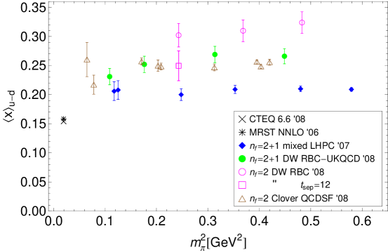
Figure 116: Overview of dynamical lattice QCD results for the isovector quark momentum fraction in the $\overline{\text{MS}}$ scheme at a scale of $4\text{ GeV}^{2}$.

Notably, there are substantial discrepancies visible in the overall normalizations of some of the lattice results in Fig. 116. In particular, the $n_{f}=2$ domain wall results from RBC are on average above most other data points, and the results from the $n_{f}=2+1$ mixed action calculation by LHPC lie exceptionally low compared to the rest. Possible explanations that were proposed in the literature are related to the semi-non-perturbative operator renormalization in the case of the LHPC analysis, and contaminations from excited states. Although the chiral extrapolation of the LHPC lattice data in Fig. 85, section 4.4.2, based on covariant baryon ChPT looks very promising, the results have to be viewed with great caution as long as the normalization issues have not been resolved.

Furthermore, for a fully quantitative comparison with experimental results, the simulations have to be pushed to even lower pion masses, $m_{\pi}\lessapprox 300\text{ MeV}$, where results from chiral perturbation theory can be more safely applied and used for extrapolations to the physical point.

The lowest moments of unpolarized, polarized and tensor/transversity generalized parton distributions of the nucleon have been studied quite extensively in unquenched lattice QCD in recent years. This includes in particular the nucleon form factors of the energy momentum tensor, which are essential for an understanding of the nucleon spin structure and the decomposition of the nucleon spin in form of Ji’s sum rule, Eqs. (69,75).

An overview of results for quark spin and (orbital) angular momentum contributions from $n_{f}=2$ clover-improved Wilson fermion simulations by QCDSF [B⁺07g] and $n_{f}=2+1$ mixed action calculations by LHPC [H⁺08a] is given in Table 2, in the $\overline{\text{MS}}$-scheme for $\mu^{2}=4\text{ GeV}^{2}$.

LHPC [E⁺06a, H⁺08a] $\frac{1}{2}\Delta\Sigma$ $L$ $J=\frac{1}{2}\Delta\Sigma+L$ $u$ $0.409(34)$ $-0.195(44)$ $0.214(27)$ $d$ $-0.201(34)$ $0.200(44)$ $-0.001(27)$ $u+d$ $0.207(28)$ $0.005(52)$ $0.213(44)$

QCDSF-UKQCD [K⁺06, B⁺07g] $\frac{1}{2}\Delta\Sigma$ $L$ $J=\frac{1}{2}\Delta\Sigma+L$ $0.428(31)$ $-0.198(32)$ $0.230(8)$ $-0.227(31)$ $0.223(32)$ $-0.004(8)$ $0.201(24)$ $0.025(27)$ $0.226(13)$

Table 2: Overview of spin and angular momentum contributions of quarks to the spin of the proton. All results have been extrapolated to the physical pion mass using results from ChPT and are given in the $\overline{\text{MS}}$-scheme at $\mu=2\text{ GeV}$. The numbers have been collected from [E⁺06a, H⁺08a] for the $n_{f}=2+1$ mixed action calculation of LHPC (table on the left) and [K⁺06, B⁺07g] for the $n_{f}=2$ clover-improved Wilson fermion simulations by QCDSF/UKQCD (table on the right).

These results certainly represent a first major step towards a quantitative decomposition of the nucleon spin in full QCD. In reviewing them, we note, however, that several items should be kept in mind:

• only connected contributions are included, disconnected parts contributing in the singlet sector are missing

• since $J_{q}=(\langle x\rangle_{q}+B^{q}_{20}(0))/2$, the results are in principle affected by the discrepancy in the normalization of the quark momentum fraction of results from QCDSF and LHPC (see Fig. 116 and discussion above)

• different types of chiral extrapolations were used: leading order (self-consistently improved) HBChPT for $\Delta\Sigma^{u+d}$, HBChPT with explicit $\Delta$-DOFs (SSE) for $g_{A}=\Delta\Sigma^{u-d}$, and covariant BChPT at leading order $\mathcal{O}(p^{2})$ (partially including NLO $\mathcal{O}(p^{3})$ corrections) for the form factors of the energy-momentum-tensor

• the lowest pion masses are $\gtrapprox 350\text{ MeV}$, where the applicability of ChPT is not established

Nevertheless, the present results show some highly remarkable features. Most prominently, the total (up- plus down-) quark orbital angular momentum contribution to the nucleon spin turns out to be very small and fully compatible with zero within statistical errors. Interestingly, the individual OAM contributions from up- and down-quarks are sizeable but of opposite sign and only cancel in the sum. These findings are at first sight completely at odds with expectations from relativistic quark models. Noting that the quark models generically live at a low hadronic scales, the results may however be reconciled if the scale evolution of OAM is taken into account.

Secondly, the down-quark angular momentum contribution is also very small and zero within errors. Again, this can be seen as the result of a precise cancellation, in this case of the individual spin and OAM contributions, which are separately non-zero and of the same size, but opposite in sign. Another interesting outcome is the observed near cancellation of the individually sizeable up- and down-quark contributions to the anomalous gravitomagnetic moment $B_{20}(t\text{{=}}0)$. If confirmed in future studies, this would not only be theoretically very interesting, but also have far reaching consequences for the gluon contributions to the nucleon spin, since from Noethers theorem $\sum_{q}B^{q}_{20}(t\text{{=}}0)+B^{g}_{20}(t\text{{=}}0)=0$.

In addition to the form factors of the energy momentum tensor that coincide with the $x$-moments of the unpolarized GPDs, also the next higher moments of GPDs have been studied. From a comparison of the lowest three $x^{n-1}$-moments, i.e. for $n=1,2,3$, it was found that the the slopes of the corresponding generalized form factors as functions of the momentum transfer squared $t$ decrease with increasing $n$, see, e.g., Fig. 104. Transformed to coordinate (impact parameter) space, this corresponds to a mean square radius of the nucleon that is rapidly decreasing as the longitudinal quark momentum fraction increases, i.e. as $x\rightarrow 1$, see Fig. 106. Since the absolute values of the generalized form factors do not enter in this case, this result is also unaffected by the normalization issue discussed above.

From first lattice studies of moments of tensor generalized parton distributions of the pion and the nucleon, qualitatively important insights were gained with respect to the distribution of transversely polarized quarks inside hadrons. The observed large values for some of the tensor GFFs point towards strong correlations between transverse spin and coordinate degrees of freedom, which in turn lead to characteristically deformed impact parameter densities of quarks with transverse polarization in unpolarized and transversely polarized hadrons, cf. Figs. 110 and 115. Specifically, it was found that the (spin-$0$) pion has a quite non-trivial transverse spin structure.

Finally, in order to be able to provide quantitatively reliable results and solid predictions for experiment, contributions from quark line disconnected diagrams will have to be consistently included in unquenched lattice calculations of flavor singlet quantities. This is a real challenge, and first promising attempts based on stochastic methods and including noise reduction techniques will be discussed below in section 6.0.2.

In the course of full calculations in the flavor singlet sector, it will also be important and necessary because of operator mixing to study the corresponding gluon observables, in particular the momentum fraction carried by gluons, as well as their spin and total angular momentum contributions to the hadron spin. First attempts in this direction have been reported already more than 10 years ago [Man90, G⁺97b], but only recently some groups show renewed interest in this subject [MN08, D⁺08b].

5 Lattice results on hadronic distribution amplitudes

5.1 Moments of meson distribution amplitudes

In this section, we briefly report on lattice QCD results for the lowest moments of meson and nucleon distribution amplitudes (DAs).

Moments of meson distribution amplitude were first studied in the late 1980’s in quenched [GK86, MS87a, DL88], and already a few years later in unquenched lattice QCD [DGR91]. The early calculations of the $\xi^{2}$-moment of, e.g., the pion distribution amplitude, $\langle\xi^{2}\rangle_{\pi}$ (see Eq. 78), were mostly based on lattice operators of the form

$$\mathcal{O}^{5DD}_{\{\mu\nu\rho\}}=\overline{q}\gamma_{5}\gamma_{\{\mu}{D^{\raisebox{2.41112pt}{$\scriptstyle\leftrightarrow$}}}{}_{\nu}{D^{\raisebox{2.41112pt}{$\scriptstyle\leftrightarrow$}}}{}_{\rho\}}q-\text{traces}$$ (164)

with $\nu=\rho$, $\mu\neq\nu$, transforming according to the 8-dimensional representation $\tau_{2}^{(8)}$ of $H(4)$. Operators of the type $\mathcal{O}^{5DD}_{\{\mu\nu\rho\}}$ with $\mu$, $\nu$ and $\rho$ all different, belonging to $\tau_{3}^{(4)}$ were also investigated in some cases (concerning the classification of the operators, see [G⁺96a]). Results of a calculation of $\langle\xi^{2}\rangle_{\pi}$ in the quenched approximation purely based on operators of type $\mathcal{O}^{5DD}_{\{\mu\nu\rho\}}$ (with all indices different) were presented in [DDDPD03]. The mixing properties of these operators were studied more recently in some detail in [G⁺05f], where also the mixing coefficients were calculated in lattice perturbation theory at the one-loop level. It was found in particular that the operator of type $\mathcal{O}^{5DD}_{\{\mu\nu\nu\}}$ mixes with a lower dimensional operator of type

$$\mathcal{O}^{D}_{\mu\nu\omega}=\overline{q}\sigma_{\mu\nu}{D^{\raisebox{2.41112pt}{$\scriptstyle\leftrightarrow$}}}{}_{\omega}q\,,$$ (165)

giving rise to power divergences of the form $1/a$ in the renormalization procedure, which would have to be subtracted non-perturbatively. On the other hand, the operators $\mathcal{O}^{5DD}_{\{\mu\nu\rho\}}$ (with all indices different) only mix with operators of the same dimension of type

$$\mathcal{O}^{5\partial\partial}_{\{\mu\nu\rho\}}=\partial_{\{\nu}\partial_{\omega}(\overline{q}\gamma_{\mu\}}\gamma_{5}q)$$ (166)

[G⁺06b]. Although at least two non-zero components of the hadron momentum are required for the evaluation of matrix elements of these operators, leading in general to more noisy correlators, they probably still represent the safer alternative for the extraction of, e.g., $\langle\xi^{2}\rangle_{\pi}$, due to the absence of mixing with lower-dimensional operators.

5.1.1 Pseudoscalar mesons

An extensive study of the lowest moments of the pion and kaon DAs, Eqs. (76) to (79), has been performed by QCDSF for $n_{f}=2$ flavors of clover-improved Wilson fermions, for pion masses in the range of $\approx 600\text{ MeV}$ to $\approx 1200\text{ MeV}$, up to four different values of the coupling $\beta=5.20,5.25,5.29,5.40$ corresponding to lattice spacings from $\approx 0.07\text{ fm}$ to $\approx 0.12\text{ fm}$, and volumes of $V\approx(1.5,\ldots,2.2\text{ fm})^{3}$ [B⁺06d]. The calculations were based on the axial-vector counterparts of the lattice operators in Eqs. (116) and (117) for the $\xi$-moment of the kaon DA, $\langle\xi\rangle_{K}$, and on an operator of the type $\mathcal{O}^{5DD}_{\{\mu\nu\rho\}}$ as discussed above for the $\xi^{2}$-moments of the pion and kaon DAs. All lattice operators were non-perturbatively renormalized, apart from the mixing with the operator $\mathcal{O}^{5\partial\partial}_{\{\mu\nu\rho\}}$, for which a perturbatively calculated mixing coefficient was used [G⁺06b]. Both types of pion (and kaon) interpolating fields as given in Eq. (96) with $\gamma_{5}$ and $\gamma_{4}\gamma_{5}$ were employed in the numerical calculations.

Figure 117: Lattice spacing dependence of the $\xi^{2}$-moment of the pion distribution amplitude (from [B⁺06d]).

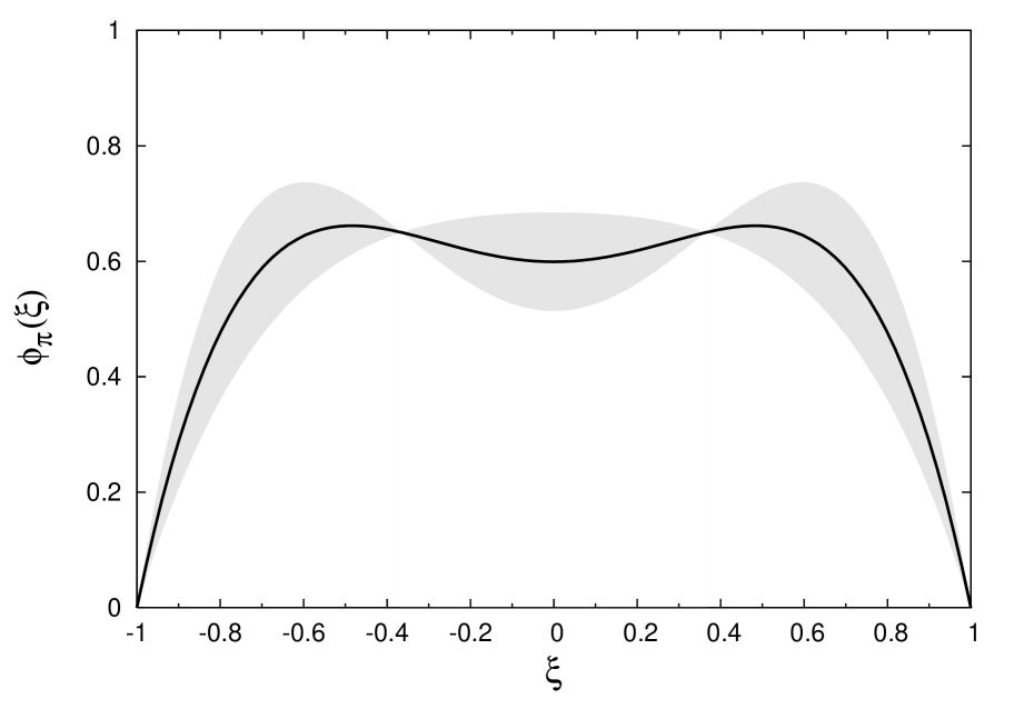
Figure 118: The pion distribution amplitude $\phi_{\pi}(\xi)$ (from [B⁺06d]).

For the case of the pion, the moments $\langle\xi^{2}\rangle_{\pi}$ were first linearly extrapolated in $m_{\pi}^{2}$ to the physical pion mass for each $\beta$. The results are plotted in Fig. 118 versus $a^{2}$, where the lattice spacings of the four data points correspond to chirally extrapolated values at the physical pion mass. Within statistical uncertainties, there is no clear lattice spacing dependence visible, and from a linear extrapolation in $a^{2}$ to the continuum limit, a value of $\langle\xi^{2}\rangle_{\pi}=0.269(39)$ was obtained in the $\overline{\text{MS}}$ scheme at a scale of $\mu=2\text{ GeV}$, which is somewhat larger than the asymptotic value $\langle\xi^{2}\rangle^{\mu\rightarrow\infty}=0.2$. An illustration of the pion distribution amplitude $\phi_{\pi}(x)$, based on this numerical result and the Gegenbauer-expansion in Eq. (80) in combination with the relation $a_{(n=2)}^{\pi}=35\langle\xi^{2}\rangle_{K}/12-7/12$, is shown in Fig. 118, where the higher Gegenbauer moments have been set to zero by hand. The shaded band represents the statistical error for $\langle\xi^{2}\rangle_{\pi}$, and it should be noted that contributions from higher moments $a_{(n>2)}^{\pi}$ may change the shape of the DA significantly.

The moments of the kaon distribution amplitude $\langle\xi\rangle_{K}$ and $\langle\xi^{2}\rangle_{K}$ were also computed in the framework of this analysis for a fixed coupling of $\beta=5.29$. Results for $\langle\xi\rangle_{K}$ are given in Fig. 120 for the axial-vector counterpart of the operator $\mathcal{O}^{b}_{1234}$ in Eq. (116), as a function of the difference $m_{K}^{2}-m_{\pi}^{2}$, for a fixed sea quark mass corresponding to a hopping parameter of $k_{\text{sea}}=0.13500$. The lattice data points in Fig. 120 were obtained for a range of values of smaller ($\hat{=}m^{\text{val}}_{u,d}$) and larger ($\hat{=}m^{\text{val}}_{s}$) valence quark masses, for which also the corresponding pion masses, $m_{\pi}^{2}$, and kaon masses, $m_{K}^{2}$, were calculated. Chiral perturbation theory predicts that $\langle\xi\rangle_{K}\propto m_{s}-m_{u,d}$ [CS04], which is according to the Gell-Mann-Oakes-Renner relations, Eq. (128), proportional to the difference $m_{K}^{2}-m_{\pi}^{2}$. The lattice data points in Fig. 120 should therefore lie on a straight line, which is indeed the case to very good approximation. From a linear interpolation to the physical difference $(m^{\text{phys}}_{K})^{2}-(m^{\text{phys}}_{\pi})^{2}\approx 0.22\text{ GeV}^{2}$, indicated by the vertical line, values for $\langle\xi\rangle_{K}$ were inferred at the given sea quark mass, i.e. in this case for $k_{\text{sea}}=0.13500$. The sea-quark mass dependence in terms of $m_{\pi}^{2}$ is displayed in Fig. 120, together with a linear extrapolation to the physical point, as represented by the straight line. A final value of $\langle\xi\rangle_{K}=0.0272(5)$ in the $\overline{\text{MS}}$ scheme for $\mu=2\text{ GeV}$ was obtained by averaging over the results obtained for different lattice operators and kaon interpolating fields.

Similar calculations of the $\xi^{2}$-moment of the pion DA, based on the operator $\mathcal{O}^{5DD}_{\{\mu\nu\rho\}}$ discussed above, were also performed for $\langle\xi^{2}\rangle_{K}$. The lattice results for the different combinations of valence, $m^{\text{val}}_{u,d}$ and $m^{\text{val}}_{s}$, and sea-quark masses at fixed $\beta=5.29$ were fitted using the global ansatz $\langle\xi^{2}\rangle_{K}=c_{0}+c_{1}m_{\pi}^{2}+c_{2}m_{K}^{2}$, where $m_{K}$ corresponds to the valence quarks masses, $m_{q}^{\text{val1}}\geq m_{q}^{\text{val2}}$, and $m_{\pi}$ to the sea-quark mass. From the global fit, a value of $\langle\xi^{2}\rangle_{K}=0.260(6)$ was obtained at the physical pion and kaon masses, for a scale of $\mu=2\text{ GeV}$ in the $\overline{\text{MS}}$ scheme. Figure 122 shows an illustration of the kaon DA $\phi_{K}(\xi)$, based on the numerical lattice results for $\langle\xi\rangle_{K}$, $\langle\xi^{2}\rangle_{K}$ and the Gegenbauer-expansion in Eq. (80) with $a_{(n=1)}^{K}=5\langle\xi^{2}\rangle_{K}/3$ and $a_{(n=2)}^{K}=35\langle\xi^{2}\rangle_{K}/12-7/12$, and where all higher moments were set to zero by hand.

Figure 119: Moment of the kaon distribution amplitude $\langle\xi\rangle_{K}$ at for fixed sea quark mass (from [B⁺06d]).

Figure 120: Sea quark mass dependence of $\langle\xi\rangle_{K}$ (from [B⁺06d]).

Results for the $\xi$-moment of the kaon DA in the framework of lattice simulations with $n_{f}=2+1$ flavors of domain wall fermions and the Iwasaki gauge action have been published by RBC-UKQCD [B⁺06c]. The computations were based on non-diagonal operators of the type $\mathcal{O}^{5D}_{\{\mu\nu\}}=\overline{q}\gamma_{5}\gamma_{\{\mu}{D^{\raisebox{2.41112pt}{$\scriptstyle\leftrightarrow$}}}{}_{\nu\}}q$ with $\mu\neq\nu$ that belong to the $H(4)$ representation $\tau_{4}^{(6)}$ [G⁺96a] and that do not mix with other operators of the same or lower dimension. Both types of pion interpolating fields in Eq. (96) were used for the calculation of the correlators. Numerical results have been obtained for a lattice spacing of $a\approx 0.12\text{ fm}$, a volume of $V\approx(2\text{ fm})^{3}$, a strange quark mass that was tuned approximately to the physical value, and three different light quark masses corresponding to pion masses of $\approx 390\text{ MeV}$, $\approx 520\text{ MeV}$ and $\approx 620\text{ MeV}$ and kaon masses of $\approx 570\text{ MeV}$, $\approx 620\text{ MeV}$ and $\approx 667\text{ MeV}$. Results for the unrenormalized (bare) moment, $\langle\xi\rangle^{\text{bare}}_{K}$, are shown in Fig. 122 versus the bare light quark mass plus the residual mass in lattice units, $a(m_{u,d}+m_{\text{res}})$, with a residual mass of $am_{\text{res}}=0.003$ (the length of the fifth dimension in the DW simulations was set to $L_{s}=16$). The quark mass dependence of the lattice data points is well described by an ansatz linear in $m_{u,d}$, in agreement with the predictions from ChPT [CS04] and with the results by QCDSF displayed in Fig. 120. In the $SU(3)$ symmetric case, $\langle\xi\rangle_{K}\rightarrow 0$, which is indeed observed in Fig. 122 where the fitting curve intersects the $x$-axis close to the expected mass of the strange quark, i.e. where $m_{u,d}\sim m_{s}$. Perturbatively calculated renormalization constants were employed to transform the results of the linear fit, represented by the solid lines in Fig. 122, to the $\overline{\text{MS}}$ scheme at a scale of $\mu=2\text{ GeV}$, giving $\langle\xi\rangle_{K}=0.032(3)$. This value is in reasonable agreement with the result of the $n_{f}=2$ Wilson fermion study by QCDSF/UKQCD discussed above, taking into account potential discretization errors and finite size effects on both sides.

Preliminary results for $\langle\xi\rangle_{K}$ and $\langle\xi^{2}\rangle_{\pi,K}$, obtained in the framework of simulations with $n_{f}=2+1$ flavors of domain wall fermions, for a lattice spacing of $a=1.729(28)\text{ fm}$, a larger volume of $V\approx(2.7\text{ fm})^{3}$, and including a lower pion mass of $m_{\pi}\sim 330\text{ MeV}$, were presented more recently by RBC/UKQCD in [B⁺08d] (see also [D⁺07]). All operators were perturbatively renormalized, including the mixing of operators of type $\mathcal{O}^{5DD}_{\{\mu\nu\nu\}}$ with the operators $\mathcal{O}^{5\partial\partial}$, as required for the calculation of the $\xi^{2}$-moments and discussed at the beginning of this section.

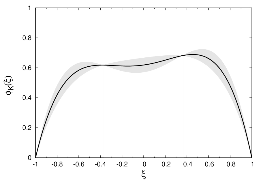
Figure 121: Illustration of the kaon distribution amplitude (from [B⁺06d]).

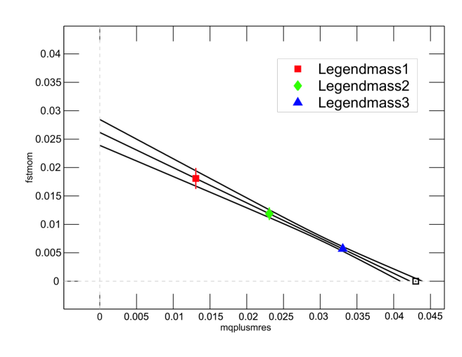
Figure 122: Chiral extrapolation of $\langle\xi\rangle_{K}$ (from [B⁺06c]).

The preliminary results, which were linearly extrapolated to the physical masses, are $\langle\xi\rangle_{K}=0.0289(19)$ and $\langle\xi^{2}\rangle_{K}=0.267(17)$ for the moments of the kaon DA, and $\langle\xi^{2}\rangle_{\pi}=0.272(20)$ for the moment of the pion DA in the $\overline{\text{MS}}$ scheme at a scale of $\mu=2\text{ GeV}$, again in good agreement with the $n_{f}=2$ Wilson fermion results from QCDSF/UKQCD[B⁺06d].

5.1.2 Vector mesons

First results for the $\xi$-moment of the (spin-1) $K^{*}$-meson DAs, $\phi_{\|}(\xi)$ and $\phi_{\perp}(\xi)$, see section 2.1.9, calculated in the framework of simulations with $n_{f}=2$ flavors of clover-improved Wilson fermions, were presented by QCDSF/UKQCD in [B⁺07e]. This preliminary study was restricted to a small subset of all available ensembles, specifically to a fixed coupling of $\beta=5.29$, (sea quark) pion masses in the range of $\approx 630\text{ MeV}$ to $\approx 1100\text{ MeV}$, and various valence quark masses. For the study of $\langle\xi\rangle^{\|}_{K^{*}}$, operators analogous to (116) and (117) were employed, and the transverse moment $\langle\xi\rangle^{\perp}_{K^{*}}$ was extracted using tensor operators (corresponding to two different $H(4)$ representations) of the form $\mathcal{O}^{\perp D}_{ij4}+\mathcal{O}^{\perp D}_{i4j}-\mathcal{O}^{\perp D}_{4ij}-\mathcal{O}^{\perp D}_{4ji}$ with $i\neq j$, and $\mathcal{O}^{\perp D}_{i44}-\sum_{j\not=i}\mathcal{O}^{\perp D}_{ijj}/2$, where $\mathcal{O}^{\perp D}_{\mu\nu\tau}=\overline{q}\gamma_{\mu}\gamma_{\nu}{D^{\raisebox{2.41112pt}{$\scriptstyle\leftrightarrow$}}}{}_{\tau}u$. They were non-perturbatively renormalized, and the final results were transformed to the $\overline{\text{MS}}$ scheme at a scale of $\mu=2\text{ GeV}$. Analogously to the pseudoscalar kaon results displayed in Fig. 120, the lattice results for $\langle\xi\rangle^{\|,\perp}_{K^{*}}$ were first interpolated to the physical value of the difference of the squared pseudoscalar kaon and pion masses, $m_{K}^{2}-m_{\pi}^{2}$, for a fixed sea quark mass but varying valence quark masses, and then linearly extrapolated in $m_{\pi}^{2}$ (corresponding to the sea quarks) to the chiral limit, giving $\langle\xi\rangle^{\|}_{K^{*}}\approx 0.033\pm 0.005_{\text{stat+sys}}$ and $\langle\xi\rangle^{\perp}_{K^{*}}\approx 0.030\pm 0.008_{\text{stat+sys}}$, where the errors represent statistical and systematic uncertainties of the calculation.

Corresponding results for the lowest two moments $\langle\xi^{(n=1,2)}\rangle^{\|}$ of $K^{*}$-, $\rho$- and $\phi$-vector meson DAs were more recently presented by RBC-UKQCD [B⁺08d]. The calculations were performed in the same lattice framework (with $n_{f}=2+1$ flavors of domain wall fermions) as already discussed in the context of pseudoscalar mesons in the previous section. Employing perturbatively renormalized operators, values of $\langle\xi\rangle^{\|}_{K^{*}}\approx 0.0324\pm 0.0016_{\text{stat}}\pm 0.0021_{\text{sys}}$ and $\langle\xi^{2}\rangle^{\|}_{K^{*}}\approx 0.248\pm 0.017_{\text{stat}}\pm 0.012_{\text{sys}}$ were obtained from linear extrapolations to the physical masses, in the $\overline{\text{MS}}$ scheme at $\mu=2\text{ GeV}$ (for a volume of $V\approx(2.7\text{ fm})^{3}$). We note that the result for $\langle\xi\rangle^{\|}_{K^{*}}$ is, within errors, perfectly compatible with the value from QCDSF/UKQCD [B⁺07e] discussed above.

5.2 Moments of nucleon distribution amplitudes

Recently, the lowest moments of the leading twist-2 nucleon distribution amplitude $\varphi(x_{1},x_{2},x_{3})$, see section 2.1.9 and Eq. (82), were studied for the first time in lattice QCD by QCDSF UKQCD [G⁺08c]. Calculations were performed using $n_{f}=2$ flavors of clover-improved Wilson fermions, for two couplings $\beta=5.29$ and $\beta=5.40$, corresponding to chirally extrapolated lattice spacings of $\approx 0.075\text{ fm}$ and $\approx 0.067\text{ fm}$, respectively, pion masses in the range of $\approx 380\text{ MeV}$ to $\approx 1200\text{ MeV}$, and volumes $V=L^{3}$ with $m_{\pi}L\geq 3.7$. Special care was taken to properly account for possible mixings of the relevant three-quark lattice operators. These baryonic operators of half-integer spin can be classified according to the so-called spinorial hypercubic group $\overline{H}(4)$, as compared to the hypercubic group $H(4)$ that is relevant for the quark- anti-quark lattice operators of integer spin, defining the moments of PDFs, GPDs and meson DAs. As in the case of the $\overline{q}q$-operators, three-quark lattice operators that transform identically with respect to $\overline{H}(4)$ can and do mix in general under renormalization. The transformation properties of the three-quark operators with up to two derivatives were studied in detail in [KGS08], where the multiplets of operators belonging to the irreducible representations $\tau_{1,2}^{\underline{4}}$ of dimension 4, $\tau^{\underline{8}}$ of dimension 8, and $\tau_{1,2}^{\underline{1}2}$ of dimension 12, have been worked out explicitly. These results were exploited in the lattice study [G⁺08c] by choosing sets of lattice operators that keep operator-mixing at a minimum and in particular avoid mixing with lattice operators of lower mass dimension, which would introduce power divergences of the form $1/a$. The corresponding twist-$2$ operators with maximally two covariant derivatives were non-perturbatively renormalized, and the results for the moments of the proton DA have been transformed to the $\overline{\text{MS}}$ scheme at a scale of $\mu=2\text{ GeV}$ [G⁺09].

Instead of the moments of the standard nucleon DA $\varphi^{klm}$ in Eq. (82) [Dzi88], a different linear combination of moments of the vector, axial-vector and tensor DAs, denoted by $\phi^{klm}$, with normalization $\phi^{000}=1$, was used, which is related to the standard DA by $\varphi^{klm}=2\phi^{klm}-\phi^{mlk}$. To reduce the substantial statistical noise for the higher moments, it turned out to be beneficial to construct normalized lattice moments (ratios) of the form $R^{klm}=\phi^{klm}/\overline{\phi}_{k+l+m}$ with $\overline{\phi}_{1}=2\phi^{100}+\phi^{010}+\phi^{001}$ and $\overline{\phi}_{2}=2(\phi^{110}+\phi^{101}+\phi^{011})+(\phi^{200}+\phi^{020}+\phi^{002})$.

Exemplary pion mass dependences of bare (unrenormalized) lattice results for the “decay constant”, $f_{N}$, and an “asymmetry” constructed from the normalized $(k+l+m=2)$-moments, $R^{200}-R^{020}=(\phi^{200}-\phi^{020})/\overline{\phi}_{2}$ are displayed in Fig.124. In the limit of infinitely large scale, $\phi(x_{1},x_{2},x_{3})\stackrel{{\scriptstyle\mu\rightarrow\infty}}{{\longrightarrow}}120x_{1}x_{2}x_{3}$, giving, e.g., $\phi^{200}=\phi^{020}=\phi^{002}=1/7$, so that the clearly non-zero asymmetry $\propto(\phi^{200}-\phi^{020})$ in Fig. 124 provides non-trivial information about deviations from the asymptotic form of the DA. Within statistics, the lattice data points lie to a good approximation on straight lines. Fits linear in $m_{\pi}^{2}$, as represented by the error bands in Fig. 124, were performed and used in particular to extrapolate all lattice results for the ratios $R^{100},\ldots,R^{001}$, $R^{110},R^{101},R^{011}$ and $R^{200},\ldots,R^{002}$ to the physical pion mass.

Finally, the moments $\phi^{klm}$ with $(k+l+m=1,2)$ were extracted from the chirally extrapolated ratios by demanding momentum conservation for the renormalized, extrapolated values, $\overline{\phi}^{\text{ren,extr}}_{1,2}\stackrel{{\scriptstyle!}}{{=}}1$, i.e. by setting $\phi^{klm}_{\text{ren,extr}}=R^{klm}_{\text{ren,extr}}$. Explicit results for the these moments with $(k+l+m=1,2)$ can be found in [G⁺08c, B⁺08g].

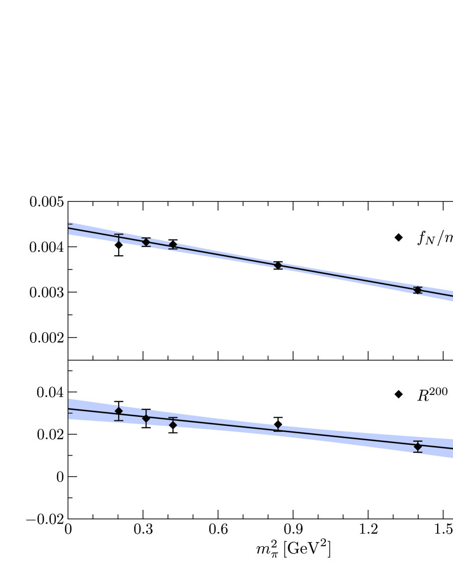
Figure 123: Decay constant and second moment of the nucleon distribution amplitude (from [G⁺08c]).

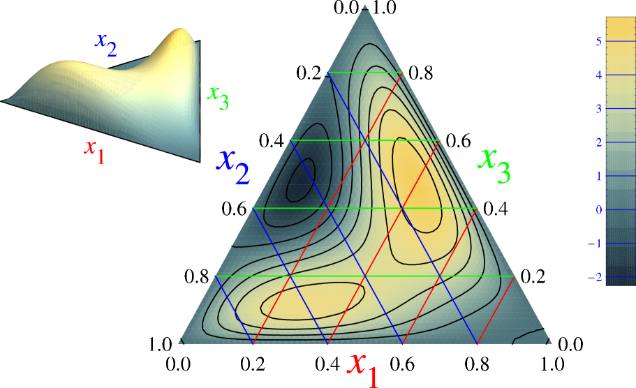
Figure 124: Illustration of $\varphi(x_{1},x_{2},x_{3})$ as obtained from the lattice results for the lowest moments of the nucleon distribution amplitude (from [G⁺08c]).

To get a first impression about possible deviations of the nucleon DA $\varphi(x_{1},x_{2},x_{3})$ from its asymptotic shape, an expansion of the form

$$\varphi(x_{1},x_{2},x_{3},\mu)=120x_{1}x_{2}x_{3}\sum_{n=0}^{N}c_{n}(\mu_{0})P_{n}(x_{1},x_{2},x_{3})\left(\frac{\alpha_{s}(\mu)}{\alpha_{s}(\mu_{0})}\right)^{\frac{3}{11N_{c}-2n_{f}}\gamma_{n}}$$ (167)

was used, where the anomalous dimensions $\gamma_{n}$ and the polynomials $P_{n}(x_{1},x_{2},x_{3})$ are given by the eigenvalues and eigenfunctions, respectively, of the three-quark-operator evolution matrix [BDKM99]. Setting higher order contributions with $n>2$ to zero, the non-perturbative coefficients $c_{n}(\mu_{0}=2\text{ GeV})$ with $n\leq 2$ in Eq. (167) were calculated from the lattice data for the moments of the DA, $\phi^{klm}_{\text{ren,extr}}$ with $(k+l+m=1,2)$, obtained for the ensemble with $\beta=5.40$. An illustration of the resulting $x_{i}$-dependencies of $\varphi(x_{1},x_{2},x_{3})$ from the truncated expansion in Eq. (167) is displayed in Fig. 124 in form of a barycentric contour plot (note that $\sum x_{i}=1$). In contrast to the asymptotic case, where the DA has a single maximum at $x_{i}=1/3$, the inclusion of the $(k+l+m=2)$-moment in particular leads the two offset local maxima and thereby a non-trivial distribution of the quark momentum.

6 Recent developments and work in progress

6.0.1 Deformation of hadrons from density-density correlators

An investigation of the deformation of hadrons based on density-density correlators was recently presented by the Cyprus group [AK08]. The study was based on equal-time four-point correlators as in Eq. 142, $C(\mathbf{r}=\mathbf{x},t_{1})=C^{00}_{\text{4pt}}(\mathbf{x},t_{1}=t_{2})$, for the pion, the $\rho$-meson, the nucleon, and the $\Delta$-baryon. All-to-all propagators and the “one-end-trick” (see section 2.3.3), which was extended to four-point-functions, were used for the first time for the calculation of four-point correlators. In what was called the “direct” method, the all-to-all propagators were replaced by their stochastic estimates, Eq. LABEL:stochastic1, based on $Z(2)$ noise vectors. Dilution in color, spin, and space (even-odd dilution) was employed to reduce the stochastic noise. For the meson correlators, the direct method was compared to calculations based on the “one-end-trick”. Calculations were performed for $n_{f}=2$ flavors of Wilson fermions for pion masses of $m_{\pi}\approx 384\text{ MeV},509\text{ MeV}$ and $\approx 691\text{ MeV}$, lattice spacing of $a\approx 0.077\text{ fm}$ and a volume of $V\approx(1.85\text{ fm})^{3}$. Gaussian smeared sources with HYP smeared gauge links were employed to improve the ground state signals and suppress contributions from excited states. The density-density operator insertion time $t_{1}$ was chosen to be centered between sink and source times, $\Delta t=t_{1}-t_{\text{src}}=t_{\text{snk}}-t_{1}$, allowing to extract a time-independent correlator at large $\Delta t$, $C(\mathbf{r})=\lim\displaylimits_{\Delta t\to\infty}C(\mathbf{r},t_{1})$. In a first step, it was shown that the use of the “one-end-trick” leads indeed to a significant improvement in the statistical precision of $C_{\pi,\rho}(\mathbf{r})$ compared to the direct method. However, it was noted that the density-density correlators could be rather sensitive to finite size effects. Due to the finite box size and the periodic boundary conditions, the correlator represents a sum over all periodic images, $C(\mathbf{r})=\sum_{\mathbf{n}}C_{0}(\mathbf{r}+L\mathbf{n})$. This must be taken into account in the interpretation of the results particularly for large distances $|\mathbf{r}|$. In a first attempt to correct for these finite size effects, the nearest neighbor contributions $C_{0}(\mathbf{r}+L\mathbf{n})$ with $|\mathbf{n}|_{\text{max}}=\sqrt{3}$ were included. The lattice correlator $C(\mathbf{r})$ was fitted using spherically symmetric (for the pion and nucleon) and non-symmetric (for the $\rho$ and $\Delta$) ansätze for the $\mathbf{r}$-dependence of $C_{0}(\mathbf{r})$ with up to five free parameters, and corrected correlators were finally obtained by a subtraction of the nearest neighbor periodic images. Results for the $\rho$-meson are displayed in Figs. 126 and 126 for the spin projections $s_{z}=0$ and $s_{z}=\pm 1$, respectively, in form of surface-plots with $\mathbf{r}$ fixed by $C_{\rho}(\mathbf{r})=C_{\rho}(\mathbf{r}=0)/2$.

Figure 125: Surface plot of the density-density correlator $C_{\rho}(\mathbf{r})$ for the $\rho$-meson with spin projection $s_{z}=0$ for $m_{\pi}=509\text{ MeV}$ (from [AK08]). The darker shaded surface corresponds to all $\mathbf{r}$ with $C_{\rho}(\mathbf{r})=C_{\rho}(\mathbf{r}=0)/2$, intersected by the lighter shaded sphere with a radius of $|\mathbf{r}|\approx 0.5\text{ fm}$.

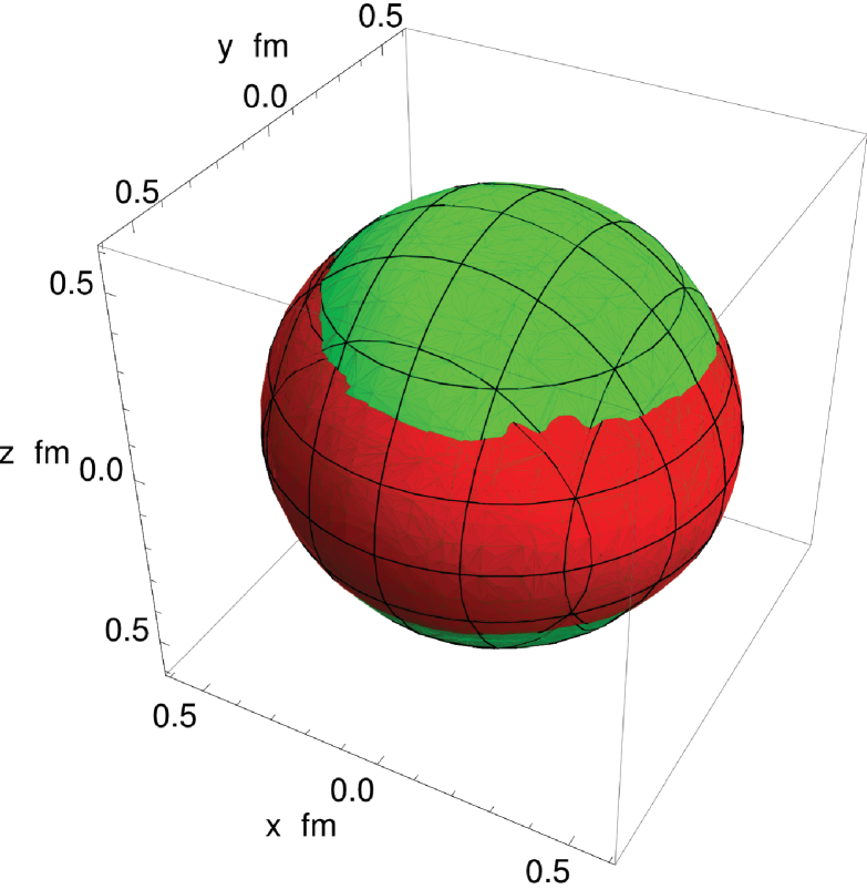
Figure 126: Surface plot of the density-density correlator of the $\rho$-meson with spin projection $s_{z}\pm 1$ for $m_{\pi}=509\text{ MeV}$ (from [AK08]). Surfaces are as described in the caption of Fig. 126.

Compared to the lighter (green) shaded spheres, the darker shaded (red) surfaces are clearly deformed in $z$-direction, pointing towards a prolate shape for $s_{z}=0$ and oblate shape for $s_{z}=\pm 1$.

In the case of the $\Delta$-baryon, where the one-end-trick could not be applied, no clear spatial deformations could be observed within the available statistics.

The results presented in Figs. 126 and 126 are certainly very promising. However, the procedure to remove the periodic images introduces a systematic uncertainty due to fit-ansätze for the $\mathbf{r}$-dependence of $C_{0}(\mathbf{r})$. It would therefore be very interesting to consider larger volumes, and to investigate the influence of these ansätze on the final results in some more detail.

6.0.2 Disconnected contributions

Quark line disconnected contributions to three-point functions, as illustrated in Fig. 4, have been discussed already several times throughout this report in sections 3.7.1, 4.3.2 and 4.4.3. They have been estimated, e.g., in the context of calculations of strange quark contributions to nucleon form factors [DLW98, LWW03], the quark momentum fraction and quark contributions to the nucleon spin [FKOU95, DLL95, G⁺99b, MDL⁺00, GJJ02, D⁺09], and polarizabilities [Eng07b]. Disconnected diagram contributions to quark three-point functions, also referred to as disconnected insertions (DI), are of the form $\langle G_{h}\times\text{Tr}\overline{\tilde{\mathcal{O}}}\rangle_{U}$ and measure gauge field correlations between the (vacuum subtracted) trace of an operator, $\text{Tr}\overline{\tilde{\mathcal{O}}}=\text{Tr}\tilde{\mathcal{O}}-\langle\text{Tr}\tilde{\mathcal{O}}\rangle_{U}$, and the hadron propagator $G_{h}$, see, e.g., the last line of Eq. (122). These correlations turn out to be in general small in magnitude compared to contributions from quark line connected diagrams. As has been discussed in section 2.3.3, the DIs involve all-to-all quark propagators, and stochastic methods are required for their calculation. Because of the additional stochastic noise and the relative smallness of the signal, it is a challenge to obtain statistically significant results for the disconnected contributions. Here, we briefly review some of the more recent efforts to improve the computation of disconnected diagram contributions in unquenched lattice QCD.

The Kentucky group recently reported promising results in particular for disconnected contributions to the quark momentum fraction $\langle x\rangle_{q}$ for up-, down- and strange-quarks in the nucleon [D⁺09]. Calculations were performed in the quenched approximation using 500 Wilson gauge configurations for a coupling of $\beta=6.0$ on a lattice of dimensions $16^{3}\times 24$. Contributions from quark line disconnected diagrams involving all-to-all propagators, specifically the traces of the operators $\text{Tr}\tilde{\mathcal{O}}(\tau)=\text{Tr}\{M^{-1}\tilde{K}^{\mathcal{O}}(\tau)\}$ (i.e. quark loops with operator insertion at time $\tau$, see Fig. 4), were estimated using stochastic noise methods as discussed in section 2.3.4. Up to 400 complex $Z_{2}$ noise estimators were used per gauge configuration, and a noise reduction was performed by emplyoing an unbiased subtraction based on the hopping parameter expansion [TDLY98]. A further reduction of the noise was achieved by considering the parity, charge and $\gamma_{5}$-hermiticity transformation properties of the nucleon propagator $G_{N}$ and the relevant quark loops and by subsequently combining only those parts that are expected to give a non-zero contribution. For example, the disconnected contribution to $\langle x\rangle_{q}$ can be obtained from a combination of nucleon three-point functions at zero momentum transfer, for a quark operator of non-diagonal type $\mathcal{O}^{a}_{4i}$, $i=1,\ldots,3$ (see Eq. (117)) of the form

$$C^{N,\mathcal{O}^{a}_{4i}}_{\text{3pt};\Gamma}(\tau,\mathbf{P}_{i})-C^{N,\mathcal{O}^{a}_{4i}}_{\text{3pt};\Gamma}(\tau,-\mathbf{P}_{i})=$$

$$\quad\quad\quad\quad-\big{\langle}\text{Im}\big{(}\text{Tr}\big{\{}\Gamma G_{N}(t_{\text{snk}},\mathbf{P}_{i})\big{\}}-\text{Tr}\big{\{}\Gamma G_{N}(t_{\text{snk}},-\mathbf{P}_{i})\big{\}}\big{)}\times\text{Im}\big{(}\text{Tr}\tilde{\mathcal{O}}(\tau)\big{)}\big{\rangle}_{U}\,,$$ (168)

involving only imaginary parts, while the real parts, which would contribute to the noise, have been dropped explicitely.

An important observation with respect to disconnected contributions is that the sink-time $t_{\text{snk}}$, e.g. in Eq. (168), may be easily varied, in contrast to a conventional sequential-source calculation of the connected contribution, which requires fixing $t_{\text{snk}}$, see, e.g., Eq. (123) and related discussion. Therefore, in order to increase the statistics, one may sum the three-point functions in Eq. (168) over the insertion time $\tau$, while studying the residual dependence on $t_{\text{snk}}$ [MMPT87, V⁺98, G⁺99b, D⁺09]. Introducing a fixed source-time $t_{\text{src}}$ (which may be set to zero), one finds

$$\frac{\displaystyle\sum\limits_{\tau=t_{\text{src}}+1}^{t_{\text{snk}}-1}C^{N,\mathcal{O}^{a}_{4i}}_{\text{3pt};\Gamma}(\tau,t_{\text{snk}},\mathbf{P}_{i})}{C^{N}_{\text{2pt};\Gamma}(t_{\text{snk}},\mathbf{P}_{i})}=c(\mathbf{P})\,\langle x\rangle_{q}t_{\text{snk}}\,+\,\text{const}\,+\,\cdots\,,$$ (169)

which depends linearly on $t_{\text{snk}}$, while contributions involving excited (positive and negative parity) states with energies $E^{\prime},E^{\prime\prime},\ldots$ indicated by the dots are exponentially suppressed by factors $e^{-(E^{\prime}-E)(t_{\text{snk}}-t_{\text{src}})}$. Since $c(\mathbf{P})$ is a known kinematical coefficient, the momentum fraction $\langle x\rangle_{q}$ may therefore be extracted from the slope in $t_{\text{snk}}$ of Eq. (169) in the limit $t_{\text{snk}}-t_{\text{src}}\gg(E^{\prime}-E)^{-1}$. This approach is different from the standard method where a plateau in the ratio of three- to two-point functions is sought at operator insertion times far away from sink and source, $t_{\text{snk}}-\tau\gg(E^{\prime}-E)^{-1}$, $\tau-t_{\text{src}}\gg(E^{\prime}-E)^{-1}$, and where contributions from excited states are suppressed by factors of $e^{-(E^{\prime}-E)(t_{\text{snk}}-\tau)}$ and $e^{-(E^{\prime}-E)(\tau-t_{\text{src}})}$, see, e.g., Eq. (110). Contributions from excited states close to source and sink are included in the sum over $\tau$ in Eq. (169), and in practice it should be checked if they are sufficiently suppressed for the accessible source-sink separations $t_{\text{snk}}-t_{\text{src}}$.

Calculations were performed for three different quark masses (hopping parameters) with $m_{u}=m_{d}$, corresponding to pion masses of $\approx 478\text{ MeV}$, $\approx 538\text{ MeV}$ and $\approx 650\text{ MeV}$, with a lattice spacing of $a\approx 0.11\text{ fm}$ that was set using the nucleon mass. The lattice operators were perturbatively renormalized and transformed to the $\overline{\text{MS}}$-scheme at a scale of $\mu=2\text{ GeV}$.

Results for the summed ratio, Eq. (169), as a function of $t_{\text{snk}}$ are displayed in Fig. 128 for a pion mass of $\approx 650\text{ MeV}$. Unbiased subtraction and the use of up to 16 nucleon sources was essential to obtain a clean signal and to increase the statistics. The slope, i.e. the momentum fraction, was extracted from a correlated fit to the lattice data points (open circles) in the range of $t_{\text{snk}}=10,\ldots,14$ as indicated by the solid line in Fig. 128, giving a clearly non-zero value of $\langle x\rangle^{\text{disc}}_{q}=0.016\pm 0.003$.

Figure  128 shows the quark mass ($m_{\pi}^{2}$-) dependence of $\langle x\rangle^{\text{disc}}_{u,d}$ together with linear extrapolations in $m_{q}$ to the chiral limit, represented by the dotted lines, from which a final value of $\langle x\rangle^{\text{disc,extr}}_{u,d}=0.032\pm 0.006$ was obtained for the case of 16 sources. By keeping the quark mass in the loop fixed at the largest value (corresponding to $\kappa=0.154$) and only varying the valence quark masses, the strange quark contribution to the momentum fraction in the nucleon was extracted in a similar way, giving $\langle x\rangle^{\text{extr}}_{s}=0.027\pm 0.006$. From these results, a ratio of strange to (disconnected) up quark contributions of $(\langle x\rangle_{s}/\langle x\rangle_{u})^{\text{disc,extr}}=0.88\pm 0.07$ was found.

In addition, calculations of the connected contributions to the momentum fractions were performed employing the conventional sequential source technique. From plateaus in $\tau$ of ratios of (connected) three- to two-point functions and linear extrapolations to the chiral limit, values of $\langle x\rangle^{\text{con,extr}}_{u}=0.408\pm 0.038$ and $\langle x\rangle^{\text{con,extr}}_{d}=0.148\pm 0.019$ were obtained, in overall agreement with earlier results in the quenched approximation, see, e.g., [D⁺02].

In summary, this study gives strong indications that the often neglected contributions from disconnected diagrams to, e.g., the total light quark momentum fraction in the nucleon, $\langle x\rangle_{u+d}$, may be as large as $\approx 10-20\%$. If correct, many lattice studies of isosinglet ovservables, such as quark angular momentum contributions to the nucleon spin in section 4.4.3, in which only the connected contributions were taken into account, could be affected by substantial systematic uncertainties and should therefore be re-assessed.

The above results should of course be considered with caution in particular because of the use of the quenched approximation and the linear extrapolations to the chiral limit. With respect to the extraction of the disconnected parts from slopes in $t_{\text{snk}}$, cf. Eq. (169) and Fig. 128, it would also be important to check for possible contaminations from excited states.

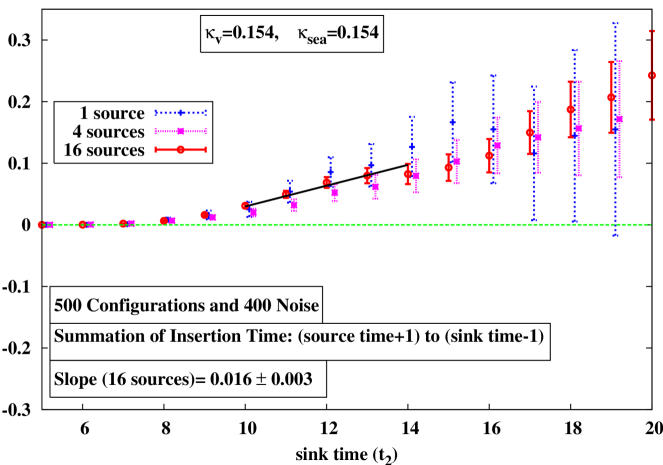
Figure 127: Summed ratio of three- to two-point functions for the disconnected insertion as a function of the sink time (from [D⁺09]).

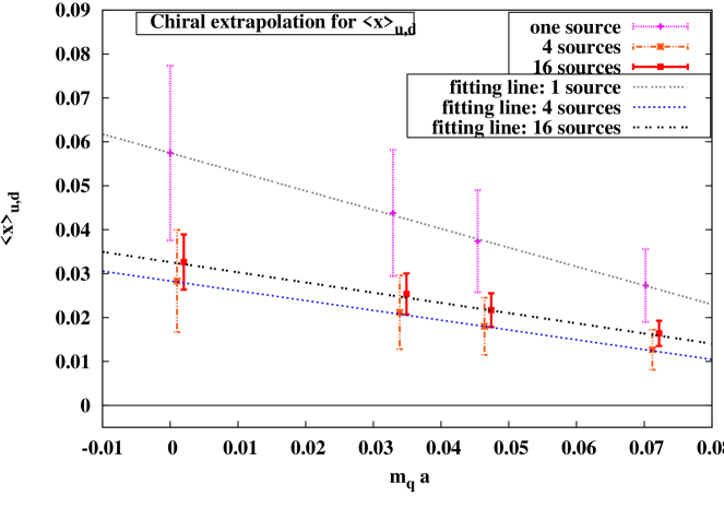
Figure 128: Quark mass dependence of $\langle x\rangle^{\text{disc}}_{u,d}$ (from [D⁺09]).

For preliminary results by the Kentucky group on disconnected and connected contributions to the quark momentum fraction obtained for $n_{f}=2+1$ Clover Wilson fermions, we refer to the proceedings [D⁺08b, MDD⁺08].

Progress in the stochastic computation of disconnected contributions based on a combination of various noise reduction methods has been reported recently in [BCS08]. Partitioning in time has been employed by setting the noise vectors equal to zero except on a single time-slice. The idea of the hopping parameter expansion (see section 2.3.3) has been implemented by noting that the lowest terms in the HPE for the Wilson action do not contribute to the trace, i.e. one can replace $\text{Tr}(\Gamma M^{-1})=\text{Tr}(\Gamma[1-\kappa\not D]^{-1})=\text{Tr}[\Gamma(\kappa\not D)^{n}M^{-1}]$, with, e.g., $n=8$ for the axial vector current, $\Gamma=\gamma_{\mu}\gamma_{5}$. In some cases, a further reduction of the noise has been achieved using the truncated eigenmode approach, as briefly discussed in section 2.3.3.

Finally, a new method called the truncated solver method (TSM) introduced in [CBS07], was used to improve the computation of the stochastic estimates. In its basic form, it is based on two independent sets (set $1$ and set $2$) of noise sources with numbers of sources equal to $N_{\eta,1}$ and $N_{\eta,2}$. The idea is to stop the iterative solver used to solve $M\phi=\eta_{1}^{(j)}$ for set $1$ before convergence is achieved, i.e. after $n_{\text{trunc}}<<n_{\text{conv}}$ iterations. Subsequently, the difference to the full converged solution can be stochastically estimated based on set $2$, giving an unbiased estimate of the propagator in the form $E[M^{-1}_{\text{conv}}]=E_{1}[M^{-1}_{\text{trunc}}]+E_{2}[M^{-1}_{\text{conv}}-M^{-1}_{\text{trunc}}]$. If the convergence behavior is such that already for small $n_{\text{trunc}}$ a result close to the converged answer is obtained, then the stochastic error may be significantly reduced by using a large number of sources in the truncated inversion, and a small number of sources for the expensive estimate of the correction to the converged results, i.e. $N_{\eta,1}>>N_{\eta,2}$.

The numerical studies in [CBS07] were based on a mixed action approach using the Wilson action for the valence fermions together with gauge configurations for $n_{f}=2+1$ stout-link improved (rooted) staggered sea quarks and a Symanzik improved gauge action, for a lattice spacing of $a\approx 0.127\text{ fm}$, and a physical volume of $V\approx(2.0\text{ fm})^{3}$. Using a standard ratio of the disconnected parts of the three-point to the two-point function, the disconnected contribution to the nucleon spin, $\Delta q^{\text{disc}}$, was estimated for three different quark masses in the quark loop and 2 different quark masses in the nucleon 2-point correlators, corresponding to pion masses in the range of $\approx 300\text{ MeV}$ to $\approx 600\text{ MeV}$. All results for $\Delta q^{\text{disc}}$ turned out to be compatible with zero. Compared to a sole partitioning in time, the use of the additional noise reduction techniques lead to absolute errors that were smaller by up to a factor of $3$, while the central values moved even closer to zero.

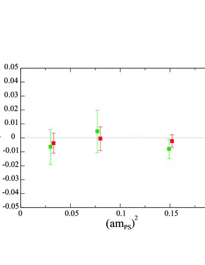
Figure 129: Unrenormalized disconnected quark contribution to the nucleon spin (from proceedings [BCS08]).

Figure 129 displays $\Delta q^{\text{disc}}$ as a function of the squared pion mass in lattice units (corresponding to the three different quarks masses in the loop). Within errors, no systematic variation of the results with the quark mass could be observed. An already quite impressive upper limit of $|\Delta s|<0.022$ at $95\%$ confidence level is found for the unrenormalized strange quark contribution to the nucleon spin at the intermediate nucleon mass. This may be compared to recent results from HERMES of $\Delta s=-0.085(13)_{\text{th}}(8)_{\text{exp}}(9)_{\text{evo}}$ obtained from inclusive DIS and using $SU(3)$ symmetry [A⁺07b], and $\Delta s^{[x=0.02-0.4]}=0.037(19)_{\text{stat}}(27)_{\text{sys}}$ from charged kaon production in semi-inclusive DIS [A⁺08d], both for the $\overline{\text{MS}}$-scheme at a scale of $5\text{ GeV}^{2}$. Keeping in mind that the experimental results generically suffer from uncertainties due to lack of data in the region of very low $x$, further improved lattice calculations (including a proper operator renormalization) might indeed have a significant impact and help to get a better quantitative understanding of strange, and possibly also the light, quark contributions to the nucleon spin in the near future.

Further preliminary results for strange quark contributions to nucleon form factors using “extremely diluted” stochastic sources have been reported by Babich et al. [B⁺07a, B⁺08a].

6.0.3 Operator product expansion on the lattice

Many hadron structure studies in lattice QCD focus on hadronic matrix elements of local operators, providing, e.g., moments of PDFs. They are related to the cross section of deep inelastic scattering (DIS), i.e. the structure functions, by the operator product expansion (OPE). The OPE of the hadronic current tensor given by the product of two electromagnetic currents can be written in momentum space as

$$W_{\mu\nu}=\langle h(P)|J_{\mu}(q)J^{\dagger}_{\nu}(q)|h(P)\rangle=\sum_{i,n}C_{\mu\nu,\{i,n\}}(q)\langle h(P)|\mathcal{O}_{\{i,n\}}|h(P)\rangle\,,$$ (170)

where in DIS $q$ is the momentum transferred by the virtual photon to the hadron $h$, $C_{\mu\nu,\{i,n\}}(q)$ are the Wilson coefficients, and $\mathcal{O}_{\{i,n\}}$ are local quark and gluon operators. Concentrating on the non-singlet sector, the sum in Eq. (170) runs over an infinite set of local quark operators,

$$\mathcal{O}_{\{i,n\}}=\mathcal{O}_{\Gamma_{i}\mu_{1}\ldots\mu_{n}}=\bar{q}\Gamma_{i}{D^{\raisebox{2.41112pt}{$\scriptstyle\leftrightarrow$}}}{}_{\mu_{1}}\cdots{D^{\raisebox{2.41112pt}{$\scriptstyle\leftrightarrow$}}}{}_{\mu_{n}}q\,,$$ (171)

where $\Gamma_{i}$ is an element of the Dirac algebra, $i=1,\ldots,16$, and $\{i,n\}$ is shorthand for the Lorentz indices and Dirac structure. The hadronic matrix elements of the local operators are parametrized in terms of moments of leading and higher twist PDFs. In the usual phenomenological approach, the Wilson coefficients $C_{\mu\nu,\{i,n\}}(q)$ are calculated to a given order in QCD perturbation theory, and are used to extract the PDFs from the measured structure functions using the OPE, Eq. 170. The moments of the PDFs obtained in this way can finally be compared to corresponding lattice results. It has, however, been noted that also the Wilson coefficients $C_{\mu\nu,\{i,n\}}(q)$ can be calculated non-perturbatively in lattice QCD [C⁺99b, C⁺99a, DL06, B⁺07d, B⁺08c]. This is feasible because they are independent of the hadron $h$ and its momentum $P$, so that off-shell quark states $|h(P)\rangle=|q(P)\rangle$ can be used to calculate the corresponding matrix elements on the left and right hand sides of Eq. (170). To get a non-zero result, this clearly has to be done in a fixed gauge, for example Landau gauge. A non-perturbative calculation of Wilson coefficients is not only interesting by itself, but could be used together with lattice determinations of nucleon matrix elements of local quark operators, discussed in section 4.3.2, to obtain fully non-perturbative results for moments of nucleon structure functions. If the Wilson coefficients and the nucleon matrix elements are calculated within the same lattice framework, their scale and scheme dependences will cancel out in the calculation of the hadronic tensor, Eq. 170. Bare lattice results may therefore be used, avoiding the costly non-perturbative renormalization of local lattice operators. Furthermore, higher twist contributions to moments of nucleon structure functions, implicitly included in the OPE in Eq. (170), may be directly accessed in the framework of a non-perturbative calculation of the Wilson-coefficients and the corresponding nucleon matrix elements of local operators [C⁺99a].

In practice, only a finite number of operators can be considered, so that the expansion in Eq. 170 has to be truncated. A truncation of terms of higher dimension, i.e. at large $n$, can be justified if the involved scales are well separated, that is if $|P^{2}|<<|q^{2}|$. At the same time, in order to keep discretization effects in a lattice calculation under control, $|q^{2}|<<(\pi/a)^{2}$. So far, operators with up to three covariant derivatives, $n=1,\ldots,n_{\text{max}}=3$, have been included in lattice QCD calculations [C⁺99b, C⁺99a, B⁺07d, B⁺08c]. The most recent study of Wilson coefficients in lattice QCD was done in the quenched approximation, using the Lüscher-Weisz gauge action with a lattice spacing of $a\approx 0.075\text{ fm}$ and a volume of $V\approx(1.8\text{ fm})^{3}$, and overlap valence quarks with a bare quark mass of $m_{q}\approx 73\text{ MeV}$ [B⁺08c]. The large number of $1360$ operators for $n_{\text{max}}=3$ could be reduced to only $67$ independent operators by choosing an isotropic momentum transfer, $q\propto(1,1,1,1)$, and using symmetry arguments [B⁺07d]. To determine the $N=67$ Wilson coefficients, off-shell quark matrix elements of the product of two electromagnetic currents, and of the local operators, were calculated for up to $M=25$ different lattice momenta $P_{i=1,\ldots,M}$. For fixed external indices, for example $\mu=\nu=4$, this leads to linear equations of the form $W_{44}(P_{i},q)=\sum_{m=1}^{67}C^{m}_{44}(q)M_{m}(P_{i})$, where $M_{m}(P)=\langle q(P)|\mathcal{O}_{m}|q(P)\rangle$, the index $m$ specifies the 67 independent operators, and $i=1,\ldots,M$. Taking also into account all $4\times 4=16$ combinations of the spinor-indices of the initial and final quark states, this provides a system of $16\times M$ equations. In the case that this system is overdetermined, i.e. that the number of linearly independent equations is larger than the number of independent Wilson coefficients, an approximate solution can be constructed using standard methods, for example the singular value decomposition.

Numerical results for the $m=1,\ldots,67$ Wilson coefficients obtained using $\mu=\nu=3$ and $\mu=\nu=4$, for a momentum transfer squared of $q^{2}\approx 17\text{ GeV}^{2}$, are displayed in Fig. 130. For orientation, we note that $m=1$ correspond to operators with zero, $m=2,\ldots,6$ with one, $m=7,\ldots,16$ with two, and $m=17,\ldots,67$ with three derivatives. Typical choices for independent operators are $\mathcal{O}_{m=1}=\overline{q}\mathds{1}q$ for zero derivatives, and $\overline{q}\sum_{i=1}^{3}\gamma_{i}D_{i}q$ for the one-derivative case. Because of chiral symmetry, the Wilson coefficients for $\mathcal{O}_{m=1}$ and for any other of the 67 operators with an even number of derivatives must vanish in the combined continuum and chiral limit. In this study, due to the use of overlap fermions, which provide an exact lattice chiral symmetry, the corresponding Wilson coefficients were expected to be small. This was indeed numerically confirmed as shown in Fig. 130, where the corresponding coefficients turn out to be suppressed.

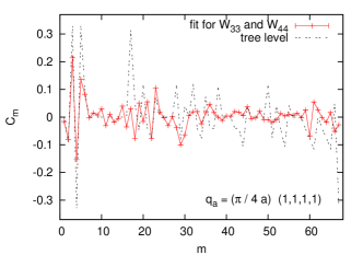
Figure 130: Wilson coefficients for operators with up to three derivatives (from proceedings [B⁺08c]).

In particular for low $m$, the lattice data points follow a pattern similar to the tree-level results given by the dashed line. This is somewhat different for larger $m$, where clear differences between the perturbative and non-perturbative results can be observed. It would be very interesting to further improve these preliminary studies by using larger sets of lattice momenta $P_{i=1,\ldots,M}$, additional momentum transfers $q$, and by including all possible combinations of the indices $\mu,\nu$. Lower $P^{2}$, and therefore a better scale separation, will be achieved by using partially twisted boundary conditions [B⁺08c].

6.0.4 Nucleon structure with partially twisted boundary conditions

Partially twisted boundary conditions (pTBCs), introduced at the end of section 2.3.3, have already been successfully employed in recent years for calculations in the meson sector, for example the kaon to pion transition form factor and the pion form factor [BFJ⁺07, B⁺08e], as discussed in section 3.3. More recently, pTBCs have been used for the first time in an exploratory study of the nucleon structure [H⁺08b]. Calculations were performed in the framework of simulations with $n_{f}=2$ flavors of non-perturbatively clover-improved Wilson fermions and the Wilson gauge action. Preliminary results were obtained for an ensemble with $\beta=5.29$ and $\kappa=0.13590$, corresponding to a lattice spacing of $a\approx 0.075\text{ fm}$, a pion mass of $m_{\pi}\approx 630\text{ MeV}$, for a spatial volume of $V=L^{3}\approx(1.8\text{ fm})^{3}$, with $m_{\pi}L\approx 5.7$. The twisting angles were chosen such that very small, non-zero values of the squared momentum transfer could be reached, $|t^{\not=0}_{\text{min}}|\simeq 0.01\text{ GeV}^{2}$, and that the large gaps of $\approx 0.5\text{ GeV}^{2}$ between the accessible Fourier momenta, $\mathbf{p}^{F}=(2\pi/(aL))\mathbf{n}$, could be filled. Figures 132 and 132 show the $t$-dependence of the isovector Dirac and the Pauli form factors, respectively. Results for standard periodic boundary conditions (“Fourier-momenta”) are given by the filled squares, while the larger number of open squares represent the lattice data points obtained with pTBCs. Dipole fits to the filled squares, and to the combined data points for $|t|\leq 1\text{ GeV}^{2}$ are shown by the gray and the blue error bands, respectively. The statistical precision of the results at low momentum transfers is quite remarkable. However, the pTBC data points above $t\sim-1\text{ GeV}^{2}$ scatter significantly, and sets of data points below $t\sim-1\text{ GeV}^{2}$ seem to be systematically lower than the average. A likely explanation are currently uncontrolled systematic uncertainties, in particular discretization effects and finite volume effects related to the pTBCs. As has been observed in [Tib06, JT08a] for the isovector magnetic moment in the framework of partially quenched ChPT, finite volume effects from pTBCs may indeed be sizeable in the nucleon sector.

From the dipole fit to the combined data points for the Dirac form factor in Fig. 132, a mean square radius of $\langle r_{1}^{2}\rangle^{u-d}=12/m_{D}^{2}=0.191(2)\text{ fm}^{2}$ was obtained, showing a substantially reduce statistical error compared to $\langle r_{1}^{2}\rangle^{u-d}=0.191(5)\text{ fm}^{2}$ for the Fourier momentum (periodic BCs) based results. A similar improvement in statistics by using pTBCs was observed for the Pauli form factor displayed in Fig. 132. Dipole fits to the combined lattice data give a mean square radius of $\langle r_{2}^{2}\rangle^{u-d}=0.259(10)\text{ fm}^{2}$ and an anomalous magnetic moment of $\kappa^{u-d}=3.101(64)$, compared to $\langle r_{2}^{2}\rangle^{u-d}=0.272(26)\text{ fm}^{2}$ and $\kappa^{u-d}=3.158(160)$ from the fit to the filled data points for the periodic boundary conditions. Even more promising, a value of $\kappa^{u-d}\approx F^{u-d}_{2}(t\approx-0.01\text{ GeV}^{2})=2.88(21)$ with a statistical error below $10\%$ could be directly obtained very close to the forward limit with pTBCs. However, as has been noted above, finite volume effects may be significant in this case, so that the results should be regarded with due caution.

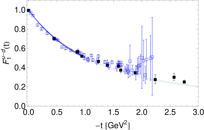
Figure 131: The Dirac form factor in the isovector channel using pTBCs (from proceedings [H⁺08b]).

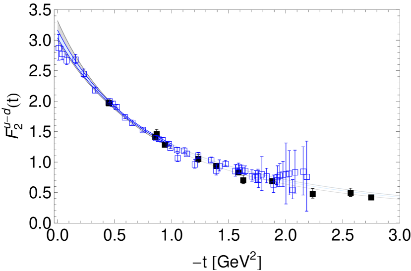
Figure 132: The Pauli form factor in the isovector channel using pTBCs (from proceedings [H⁺08b]).

Preliminary results for the nucleon generalized form factors $B_{20}(t)$, which plays a central role for the nucleon spin structure, Eq. (69), and $C_{20}(t)$, obtained using pTBCs are shown in Figs. 134 and 134 in the isovector channel. A calculation of these GFFs employing pTBCs is particularly promising, since neither $B_{20}(t)$ nor $C_{20}(t)$ can be directly obtained at zero momentum transfer, as discussed at the end of section 2.3.3.

As before, the filled squares represent the results for standard periodic BCs, and the data points obtained with pTBCs are given by the open squares. Dipole fits to the periodic BC and to the combined data points are represented by the error bands. A direct calculation of $B^{u-d}_{20}(t)$ very close to the forward limit gives $B^{u-d}_{20}(-0.02\text{ GeV}^{2})=0.402(39)$ with good statistical precision of $\sim 10\%$. Within errors, this is compatible with the values from the dipole fits of $B^{u-d}_{20}(0)=0.440(19)$ for the combined, and $B^{u-d}_{20}(0)=0.432(35)$, for the periodic BC (Fourier momentum) lattice data. Qualitatively new insights may be obtained for $C^{u-d}_{20}(t)$. In this case, the lattice data points for the periodic BCs are compatible with zero over the full range of $|t|\simeq 0.5,\ldots,3\text{ GeV}^{2}$. However, for the low values of $|t|\leq 0.5\text{ GeV}^{2}$ that could be reached with pTBCs, a trend towards non-zero, negative values can be observed in Fig. 134, albeit with rather large statistical errors.

Provided that systematic uncertainties such as finite volume effects can be brought under control, partially twisted boundary conditions hold great promise for the understanding of a large number of key nucleon structure observables.

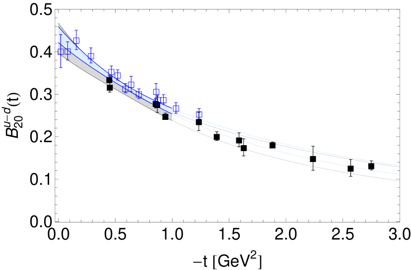
Figure 133: The form factor $B_{20}(t)$ in the isovector channel using pTBCs (from proceedings [H⁺08b]).

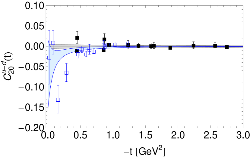
Figure 134: The form factor $C_{20}(t)$ in the isovector channel using pTBCs (from proceedings [H⁺08b]).

6.0.5 Nucleon form factors at high momentum transfer on anisotropic lattices

Lattice calculations of nucleon form factors at large values of the momentum transfer are interesting for a number of reasons. First, they might provide a better understanding of the large $Q^{2}$-scaling behavior in particular in comparison with respective predictions from perturbative QCD. Moreover, they could provide interesting predictions for planned experiments in the high-$Q^{2}$ region at, e.g., JLab. Specifically, such calculations would allow to directly investigate a possible zero-crossing of the Sachs electric form factor $G_{E}^{p}(Q^{2})$ somewhere above $Q^{2}\gtrapprox 6\text{ GeV}^{2}$ [G⁺02].

Lattice calculations of nucleon form factors at large $Q^{2}$ are challenging since they suffer in general from poor signal-to-noise ratios. They require high-momentum nucleon states, but the smearing of the sources and sinks is usually tuned to provide an optimal overlap with the nucleon ground state at rest and therefore potentially provides a rather poor overlap with a fast-moving nucleon. Furthermore, the signal-to-noise ratio of the correlators deteriorates quickly for large nucleon momenta and large times. This is particularly a problem in calculations based on standard ratios of three- to two-point functions (cf. Eq. 110) since this requires accurate knowledge of the nucleon two-point function for large source and/or sink momentum at large sink-times.

A new strategy to improve the calculation of form factors at large $Q^{2}$ on the lattice has been proposed and tested recently [LCE⁺08]. It is based on the idea of using a set of differently Gaussian smeared [AGJ⁺94] interpolating fields, including those that have a better overlap with high-$P$ and excited nucleon states, on anisotropic lattices with $a_{s}>a_{t}$. This then provides for a better resolution in the time direction and hence allows to study the exponential decay of excited and high momentum states more precisely. In this study, three different Gaussian smearing strengths have been used, and the nucleon two-point functions were calculated for all 9 possible source-sink smearing combinations. From a diagonalization of the correlators, the energies and overlap factors of the ground and first excited state could be extracted. These results were then used to extract the relevant matrix elements (and from them finally the form factors) from simultaneous fits to the three-point functions, which have also been calculated for all 9 source-sink smearing combinations. Preliminary results were obtained in the quenched approximation using the Wilson gauge action for three pion masses of $\approx 480\text{ MeV}$, $\approx 720\text{ MeV}$ and $\approx 1100\text{ MeV}$, a spatial lattice spacing of $a_{s}\approx 0.1\text{ fm}$, and with $a_{s}=3a_{t}$. As displayed in Fig. 135, an impressively clean signal was found for the Dirac form factor $F_{1}$ in the isovector channel up to rather large momentum transfers $Q^{2}\approx 5\text{ GeV}^{2}$. Similar results have been obtained for the Pauli form factor, and from the combination of $F_{1}$ and $F_{2}$ it was found that the Sachs proton electric form factor does not cross zero in the accessible region of $Q^{2}$. Further results were obtained for nucleon excited-ground state transition form factors. It would be very interesting to further improve this promising approach and to extend the calculations to unquenched QCD and even higher $Q^{2}$.

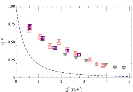
Figure 135: Isovector Dirac form factor for pion masses of $\approx 480\text{ MeV}$ (triangles) $\approx 720\text{ MeV}$ (squares) and $\approx 1100\text{ MeV}$ (downward triangles) for a large range of $Q^{2}$ (from proceedings [LCE⁺08]).

6.0.6 Transverse momentum dependent parton distribution functions in lattice QCD

We now turn to a brief discussion of another class of interesting observables, the so-called transverse momentum dependent parton distribution functions (tmdPDFs). These provide important information about hadron structure that is to a large extent complementary to the physics content of PDFs and GPDs, which have already been discussed in some detail in this report. The tmdPDFs depend, in addition to the longitudinal momentum fraction $x$, on the intrinsic transverse momentum $k_{\perp}$ carried by the quarks and gluons in the hadron, and have in general a probability density interpretation, similar to the generalized parton distributions (GPDs), which provide information about the distribution of quarks and gluons in transverse coordinate space (impact parameter-, $b_{\perp}$-space, see Eq. (64) and illustration Fig. 1). We stress, however, that the transverse momentum, $k_{\perp}$, and coordinate, $b_{\perp}$, dependent distribution functions are not directly related by a Fourier-transformation and provide in general complementary information about the structure of hadrons.

Transverse momentum dependent PDFs play a central role in the description of semi-inclusive deep inelastic scattering (SIDIS) and the Drell-Yan-process (DY-process). For a recent review, we refer to [DM08]. In such processes, correlations between the intrinsic transverse momenta of the partons, the hadron momentum, and their spins can lead to very interesting asymmetries. Prominent examples are single spin azimuthal asymmetries in SIDIS generated by the Collins- and Sivers-effect, which have been studied at HERMES, COMPASS and BELLE [A⁺05b, A⁺05d, A⁺06]. Despite the fact that tmdPDFs are phenomenologically relevant and provide important information about structure of hadrons, they received to this date very little attention in the framework of lattice QCD. One of the reasons for this may be that there is no unique and broadly accepted definition of tmdPDFs in terms of matrix elements of quark and gluon operators available. A range of definitions, some of which were proposed in the context of SIDIS-factorization, can be found in Refs. [CH00, Col03, JMY05, CM04, CS08].

For the exploratory lattice studies in [M⁺07b, M⁺08], a basic definition in terms of the correlators (see, e.g., [MT96] and references therein)

$$\Phi_{\Gamma}(x,k_{\perp};P,S)\equiv\frac{1}{2}\int d(\bar{n}\cdot k)\int\frac{d^{4}l}{(2\pi)^{4}}e^{-ik\cdot l}\ \langle P,S|\bar{q}(l)\,\Gamma\mathcal{U}_{\mathcal{C}(l,0)}\ q(0)|P,S\rangle$$ (172)

was employed, were $|P,S\rangle$ denotes a nucleon state, $\bar{n}$ is a lightlike vector with $\bar{n}\cdot n=1$, and where the Wilson line $\mathcal{U}_{\mathcal{C}(l,0)}$ guarantees the gauge invariance of the bilocal quark operator (for the notation, see also section 2.1). These correlators are, for example, parametrized by the tmdPDF $f_{1}(x,k_{\perp}^{2})$ in the unpolarized case, $\Gamma=\;\not n$, and by $g_{1L}(x,k_{\perp}^{2})$ and $g_{1T}(x,k_{\perp}^{2})$ in the polarized case, $\Gamma=\;\not n\gamma_{5}$,

$$\Phi_{\not n}(x,k_{\perp};P,S) = f_{1}(x,k_{\perp}^{2})$$

$$\Phi_{\not n\gamma_{5}}(x,k_{\perp};P,S) = \frac{m_{N}}{n\cdot P}n\cdot Sg_{1L}(x,k_{\perp}^{2})\ +\ \frac{k_{\perp}\cdot S_{\perp}}{m_{N}}\ g_{1T}(x,k_{\perp}^{2}).$$ (173)

Formally integrating over the transverse momentum, the operator in Eq. 172 reduces to the light-cone operator in Eq. (1), and one finds a direct relation to the standard PDFs,

$$q(x) = f_{1}(x)=\int d^{2}k_{\perp}f_{1}(x,k_{\perp}^{2})\;,$$

$$\Delta q(x) = g_{1}(x)=\int d^{2}k_{\perp}g_{1L}(x,k_{\perp}^{2})\;.$$ (174)

Note that the $k_{\perp}$-integrals in Eqs. (174) are logarithmically divergent, and that the upper integration limit is related to the scale-, $\mu$-, dependence of the PDFs described by the well-known DGLAP evolution equations.

The gauge link path $\mathcal{C}(l,0)$ in Eq. 172 is a crucial ingredient in the definition of tmdPDFs, and is given by the combination of three straight lines of the form $\mathcal{C}(l,0)=[l,l\pm\infty n][l\pm\infty n,\pm\infty n][\pm\infty n,0]$, where the plus and minus signs correspond to the cases of SIDIS and DY-scattering, respectively. It turns out, however, that the gauge links on the light cone lead to so-called light cone singularities in (continuum) perturbation theory, so that in fact a modified definition of the tmdPDFs is needed [CH00, Col03, JMY05, CM04, CS08].

To simplify the problem, a straight Wilson line, $\mathcal{U}_{[l,0]}$, directly connecting the quark field operators, was used for the numerical studies in [M⁺07b, M⁺08]. It is important to note that the first lattice results are therefore not directly related to the phenomenologically relevant tmdPDFs in SIDIS and DY-processes. The nucleon matrix elements in Eq. 172 can be parametrized by complex valued, invariant amplitudes $\tilde{A}_{i}(l^{2},l\cdot P)$. In the conventions of [M⁺08] one has for example

$$\langle P,S|\bar{q}(l)\gamma_{\mu}\mathcal{U}_{\mathcal{C}(l,0)}q(0)|P,S\rangle = 4\tilde{A}_{2}P_{\mu}+4im_{N}^{2}\tilde{A}_{3}l_{\mu}\;,$$

$$\langle P,S|\bar{q}(l)\gamma_{\mu}\gamma_{5}\mathcal{U}_{\mathcal{C}(l,0)}q(0)|P,S\rangle = -4m_{N}\tilde{A}_{6}S_{\mu}-4im_{N}\tilde{A}_{7}P_{\mu}l\cdot S+4m_{N}^{3}\tilde{A}_{8}l_{\mu}l\cdot S\,.$$ (175)

For the lattice calculation of the nucleon matrix elements, standard nucleon two-point and three-point functions (obtained using the sequential source technique) have been employed. The distance between the quark fields in the time direction was set to zero, $l_{0}=0$, and in the cases that the spatial separations were not directed along a single axis, the straight lines in the continuum were approximated by zigzag (step-like) paths on the lattice. Products of link variables were used to represent the Wilson lines $\mathcal{U}_{[l,0]}$ in the discretized non-local operators.

It is well known [Dor86, EH90, MMS92] that calculations in a cutoff regularized theory, for example in lattice QCD with cutoff $\Lambda=a^{-1}$, involving Wilson lines are plagued by potential ultraviolet divergences in $\Lambda\mathcal{L}$, where $\mathcal{L}$ is the length of the path. To give a physical meaning to the $l$-dependence of the correlators, the potential power divergence has to be removed by a renormalization of the lattice operator. This can be achieved by multiplication with a factor $\exp(-\delta m\mathcal{L})$ [Dor86], where $\delta m\propto a^{-1}$. The renormalization constant $a\delta m$ was estimated using leading order lattice perturbation theory, and also non-perturbatively based on a comparison of Wilson lines directed along an axis and along other directions represented by zigzag paths on the lattice (‘taxi driver method’) [M⁺07b, M⁺08]. More recently, a different renormalization procedure, employing a specific renormalization condition that involves the string potential, has been used [Mus09a]. Since the renormalization is still preliminary and not free of ambiguities, all results below have to be regarded with due caution.

The numerical computations were based on nucleon two- and three-point functions calculated by LHPC (see, e.g., [H⁺08a]) for $n_{f}=2+1$ flavors of domain wall valence fermions and Asqtad staggered sea quarks (MILC configurations), for a lattice spacing of $a\approx 0.125\text{ fm}$, a volume of $V\approx(2.5\text{ fm})^{3}$, and three pion masses of $m_{\pi}\approx 496\text{ MeV}$, $m_{\pi}\approx 596\text{ MeV}$ and $m_{\pi}\approx 759\text{ MeV}$. First lattice results at the lightest pion mass for the real parts of the amplitudes $\tilde{A}_{2}(l^{2},l\cdot P\text{{=}}0)$ and $\tilde{A}_{7}(l^{2},l\cdot P\text{{=}}0)$ for up-quarks as functions of the distance $|l|$ are displayed in Figs. 137 and 137.

Figure 136: Real part of the amplitude $\tilde{A}^{u-d}_{2}$ as a function of the distance $|l|$, obtained for a renormalization condition based on the string potential (from [Mus09a]). Similar results based on a different renormalization procedure were presented in the proceedings [M⁺08].

Figure 137: Real part of the amplitude $\tilde{A}_{7}^{u-d}$ as a function of the distance $|l|$, obtained for a renormalization condition based on the string potential (from [Mus09a]). Similar results based on a different renormalization procedure were presented in the proceedings [M⁺08].

The statistical errors of the lattice data points for $\tilde{A}_{2}(l^{2},l\cdot P\text{{=}}0)$ are remarkably small. Both amplitudes show a Gaussian like fall-off and can be phenomenologically well described using a double Gaussian fit ansatz of the form $\tilde{A}(l^{2})=A\exp(-l^{2}/\sigma_{A}^{2})+B\exp(-l^{2}/\sigma_{B}^{2})$, as represented by the solid curves and shaded error bands.

From Eqs. (172), (173) and (175), and by noting that $l\cdot P=0$ corresponds to an integration over the longitudinal momentum fraction $x$, one finds that Fourier-transformations of the amplitudes $\tilde{A}_{2}(l^{2},l\cdot P\text{{=}}0)$ and $\tilde{A}_{7}(l^{2},l\cdot P\text{{=}}0)$, as represented in practice by, e.g., the double Gaussian parametrizations, to $k_{\perp}$-space correspond to the lowest $x$-moment of the tmdPDFs $f^{sW}_{1}$ and $g^{sW}_{1T}$, respectively. The superscript $sW$ denotes the straight Wilson lines that were employed in the definition of the lattice correlators. Based on the numerical results for $\text{Re}\tilde{A}_{7}(l^{2},l\cdot P\text{{=}}0)$, Fig. 137, it turned out that the distribution $g^{sW}_{1T}(k_{\perp})$ is positive valued for up-, and negative valued for down-quarks.

In analogy to the impact parameter space density given in Eq. 65, a transverse momentum density of longitudinally polarized quarks in a transversely polarized nucleon can be defined using Eqs. 172 and 173, given by [DH05]

$$\rho(x,k_{\perp};\lambda,S_{\perp})=\Phi_{\not n(1+\lambda\gamma^{5})/2}(x,k_{\perp};P,S_{\perp})=\frac{1}{2}\left(f_{1}(x,k_{\perp}^{2})+\lambda\frac{k_{\perp}\cdot S_{\perp}}{m_{N}}g_{1T}(x,k_{\perp}^{2})\right)\,,$$ (176)

where $\lambda$ denotes the quark helicity. At this point, it is important to note that the continuum tmdPDFs $f_{1}(x,k_{\perp}^{2})$ and $g_{1T}(x,k_{\perp}^{2})$ in Eqs. (173,176) behave asymptotically like $k_{\perp}^{-2}$ and $k_{\perp}^{-4}$ [BBDM08], respectively, so that the normalization of $\rho(x,k_{\perp};\lambda,S_{\perp})$, as given by an integral over $k_{\perp}$, needs special consideration. Here, these difficulties have been evaded by the use of a Gaussian ansatz for the $l$-dependence of the amplitudes, leading to a Gaussian fall-off in momentum space.

Figure 138 shows the lowest $x$-moment of the density, obtained for the preliminary lattice results for $f^{sW}_{1}$ and $g^{sW}_{1T}$, at a pion mass of $m_{\pi}\approx 496\text{ MeV}$.

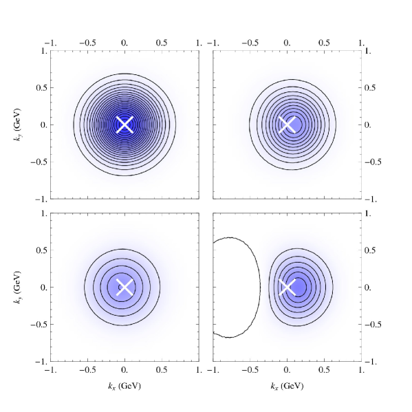
Figure 138: Lowest $x$-moment of the transverse momentum density of quarks in the nucleon (from [Mus09a], see also the proceedings [M⁺08]). Details are given in the text.

Compared to the unpolarized density (upper left corner), summed over the quark helicities $\lambda=\pm 1$, the density for up quarks with helicity $\lambda=+1$ in a transversely polarized nucleon with spin $S_{\perp}=(1,0)$ (upper right corner) is slightly deformed in $+x$-direction. This is caused by the dipole-like term $\propto k_{\perp}\cdot S_{\perp}$ in Eq. 176 and the non-vanishing positive distribution $g^{sW}_{1T}$ for up-quarks. For down-quarks, $g^{sW}_{1T}$ is negative, so that the corresponding density in the lower left corner of Fig. 138 is deformed in $-x$-direction. Clearly, the effects add up in the isovector channel displayed in the lower right corner, leading to a significant distortion of the density. We note again that the systematic uncertainties in this exploratory lattice study of the tmdPDFs $f^{sW}_{1}$ and $g^{sW}_{1T}$, in particular due to the renormalization, are still substantial, so that the results should be regarded as preliminary. Furthermore, since straight Wilson lines (“$sW$”) were employed in the correlator Eq. (172) that are significantly different from the Wilson lines of SIDIS and DY-scattering, the lattice results cannot be directly compared with or used in phenomenological studies.

7 Summary and perspectives

Due to the increasing availability and performance of supercomputers, improved methods and algorithms, as well as theoretical developments, dynamical lattice hadron structure calculations are by now routinely carried out at pion masses $\approx 350\text{ MeV}$ and below, in spatial volumes of $\approx(2\text{ fm})^{3}$ and larger. Significant efforts have been made to get discretization and finite volume effects under control.

In the course of these developments, a large number of increasingly accurate results became available, some of which have been reviewed in this report: A summary of lattice studies of form factors and polarizabilities can be found in section 3.8. Calculations of moments of PDFs and GPDs as well as distribution amplitudes are summarized and discussed in sections 4.5 and 5, respectively. Finally, in section 6, we present some promising lattice studies that are beyond mainstream.

Impressive studies of the pion form factor in unquenched lattice QCD have been published by different groups, in particular in combination with advanced methods and techniques, for example the “one-end-trick” and partially twisted boundary conditions. In a milestone calculation, $F_{\pi}(Q^{2})$ has been obtained for the first time at a non-zero momentum transfer smaller than what could be accessed so far experimentally, and with statistical errors below the experimental errors, for a comparatively low lattice pion mass of $\approx 330\text{ MeV}$. A range of different extrapolations methods, mostly based on 1- and 2-loop chiral perturbation theory, were used to get estimates of the pion charge radius at the physical point. It is noteworthy that a number of low energy constants of chiral effective field theory are extracted from such fits with increasing precision. Although the central values for $\langle r^{2}\rangle_{\pi}$ in Fig. 64 obtained from different lattice simulations and extrapolation methods still scatter significantly, they all nearly overlap within the assigned statistical and systematical uncertainties. It will be highly interesting to see if the next round of improved lattice calculations of $F_{\pi}(Q^{2})$ will finally lead to an agreement with the experimental average from the PDG.

Concerning the nucleon form factors, extensive dynamical lattice studies have been carried out in the recent years mostly based on conventional methods, reaching down to pion masses of $\approx 300\text{ MeV}$ in volumes of $\gtrapprox(2\text{ fm})^{3}$. The overview plots Fig. 65, 66 and 67 for the isovector Dirac and Pauli mean square radii and the anomalous magnetic moment, respectively, show a promising overall agreement of the lattice results, and only in some cases discrepancies between individual data points. Most remarkably, even at the lowest accessible pion masses, the lattice values for $\langle r^{2}\rangle^{u-d}_{1,2}$ are still a factor of about two below the respective experimental numbers, and a clear sign of an upwards bending is not yet visible. However, considering the ChPT predictions in Fig. 65, it is to be expected that very soon at pion masses below $300\text{ MeV}$ chiral dynamics will finally set in and lead to a non-linear increase of the radius as we approach the physical point. The unambiguous identification of the chiral singularities $\propto\log(m_{\pi}/\lambda)$ in $\langle r^{2}\rangle^{u-d}_{1}$ and $\propto 1/m_{\pi}$ in $\langle r^{2}\rangle^{u-d}_{2}$ would indeed represent a major step in our attempt to calculate these fundamental nucleon structure observables “ab initio” on the lattice.

Another benchmark observable, the nucleon isovector axial vector coupling constant $g_{A}$, received a lot of attention in recent years. Peculiar to $g_{A}$ is the importance of the $\Delta(1232)$-resonance, which is largely responsible for the deviation of $g_{A}$ from $1$, furthermore its potentially strong volume dependence, and of course the fact that its value is known very precisely from neutron beta decay. Unquenched lattice results for $g_{A}$ for a range of pion masses down to $\approx 300\text{ MeV}$, and volumes ranging from $\approx(1\text{ fm})^{3}$ to $\approx(3.5\text{ fm})^{3}$, displayed in form of a $g_{A}$-“landscape” in Fig. 68, confirm impressively the expected strong volume dependence at small $m_{\pi}\times L$. Previous lattice studies, in one case only including pion masses $\gtrapprox 600\text{ MeV}$, in the other still suffering from limited statistics, observed that the inclusion of explicit $\Delta$-intermediate states is indeed crucial for a successful chiral extrapolation, and even found agreement with the experimental number at the physical point. More recent lattice data with better statistics and at lower pion masses of $300\ldots 350\text{ MeV}$, however, does not seem to follow the previously predicted $m_{\pi}$-dependence, but is instead consistently lying $\approx 10\ldots 15\%$ below the experimental value. This suggests that the chiral extrapolations of $g_{A}$, which appeared to be quantitatively successful in the past, may have to be reconsidered in the future.

With respect to $\Delta$-intermediate states, it is also interesting to note that great progress has been made in lattice calculations of $\Delta$-baryon form factors, in particular the $\Delta$ magnetic moment, using conventional as well as background field methods. Together with similar results for nucleon-to-$\Delta$ transition form factors (which we have not discussed in this report), we may soon have the opportunity to perform simultaneous fits based on ChPT predictions to a large number of lattice data for vector and axial-vector nucleon and $\Delta$-baryon (transition) form factors. Such an approach promises a consistent and improved extraction of the relevant $NN$-, $N\Delta$- and $\Delta\Delta$-coupling constants, which appear as low energy constants in the ChPT formulae.

Important experience and knowledge has been gained in the last couple of years with respect to calculations of hadron polarizability using background field methods. For some time, apparently contradictory lattice results that differed substantially in magnitude and also in sign were presented for the neutron electric polarizability. By now, these issues seem to be settled, and consistent values for $\alpha^{n}_{E}$ obtained with different methods are available for pion masses $\gtrapprox 400\text{ MeV}$, as displayed in the overview plot Fig.70. At these pion masses, the lattice results are a factor of $3\ldots 5$ below the experimental number. Possible systematic uncertainties in these calculations certainly have to be studied in greater detail in the future. However, such low values are not entirely unexpected as ChPT predicts that the neutron electric polarizability diverges like $1/m_{\pi}$ to $+\infty$ in the chiral limit. As in the case of the nucleon mean square radii, it is a great challenge to numerically verify the presence of such singularities using lattice QCD.

Turning our attention to moments of PDFs and GPDs, we observe that the long-standing issue concerning the longitudinal momentum fraction carried by quarks in the nucleon has not yet been resolved: As displayed in Fig. 116, most of the lattice results for $\langle x\rangle_{u-d}$ are $\approx 50\%$ above the values from global PDF analyses and are practically flat in $m^{2}_{\pi}$ over a wide range of pion masses. In addition, there is in some cases a clear disagreement between individual lattice simulations. Apart from reducing the statistical errors, the central task is therefore to get the apparently substantial systematic uncertainties, related to possible discretization and finite volume effects, contaminations from excited states and the operator renormalization, finally under control. Suitable higher-order results from ChPT may in the end be crucial to a successful extrapolation of the lattice data down to the physical point.

Very valuable information about hadron structure has been obtained from lattice calculations of moments of GPDs. They provide direct access to many fundamental physics question concerning, e.g., the nucleon spin structure, the spatial distribution of partons in hadrons, and highly non-trivial correlations between the spin and coordinate degrees of freedom. Many of the corresponding observables turn out to be rather difficult to access experimentally on a quantitative level. An important example is the angular momentum carried by quarks in the nucleon, which has been calculated recently for the first time in dynamical lattice QCD. The lattice results, summarized in Table 2, are pointing towards a remarkably small total light quark orbital angular momentum, $L^{u+d}\approx 0$, and negligible total angular momentum of the $d$-quarks, $J^{d}\approx 0$. A directly related and extremely interesting question is if the anomalous gravitomagnetic moment of quarks, $B_{20}^{u+d}(t\text{{=}}0)$, is in indeed close to zero, as suggested by these first lattice studies. Most remarkably, in all the above cases, the small values turn out to be the result of quite precise cancellations between different non-vanishing flavor, spin and orbital angular momentum contributions. We stress, however, that these exciting results are currently still subject to significant systematic uncertainties, and therefore must be regarded as preliminary. In particular, contributions of so-called disconnected diagrams to singlet observables are not yet routinely included in lattice hadron structure calculations. The computation of disconnected contributions, and also gluonic hadron structure observables, remains a big challenge due to notoriously low signal-to-noise ratios. We have seen, however, renewed interest in this area and promising progress recently in particular based on a number of innovative ideas related to stochastic noise methods and noise reduction techniques.

To the class of observables that are very difficult to access in experiment also belong the tensor form factors, PDFs and GPDs, which are related to the transverse spin structure of hadrons, as well as hadronic distribution amplitudes. Dynamical lattice calculations of the former led to fascinating insights into transverse spin densities of quarks in the nucleon and the pion, showing in particular that the pion has a non-trivial spin structure.

A number of recent dynamical lattice studies provided impressive predictions for the lowest moments of meson distribution amplitudes. They are an important ingredient in the QCD-factorization of, e.g., rare $B$-meson decays (that have small branching ratios in the standard model). Since the latter are sensitive to non-standard model particles through loops, high precision lattice results might indeed provide a useful, model-independent input in the search for new physics.

Furthermore, moments of the nucleon distribution amplitude have been obtained for the first time in a sophisticated dynamical lattice study. At the present level of accuracy, the results confirm, for example, the perception that the largest momentum fraction is carried by up-valence quarks with spin parallel to that of the proton. It would be very interesting to perform further detailed studies of baryon distribution amplitudes in the future, including comparisons with QCD sum rule and model approaches.

In addition to the steady progress in calculations of classical hadron structure observables like form factors and moments of PDFs, some more unorthodox but promising ideas have been pursued in the recent years. They include a direct lattice calculation of Wilson coefficients, which may even allow to access the renormalization scale and scheme independent hadronic structure functions rather than the PDFs in the future. Progress in a new direction has been made very recently in a first lattice study of manifestly non-local quark operators, providing access to the intrinsic transverse momentum of quarks in the nucleon. This novel approach may eventually lead to lattice calculations of the phenomenologically very important transverse momentum dependent parton distributions (tmdPDfs).

One of the main limitations repeatedly encountered in lattice QCD calculations is related to very small but non-zero momentum transfers. They are required for a well-founded extraction of many fundamentally important observables, e.g., charge radii, magnetic moments and the anomalous gravitomagnetic moment. In standard lattice calculations of matrix elements, accessing a small non-zero momentum transfer of about $|Q|\simeq 0.1\text{ GeV}$ would require a very large spatial lattice volume of $V\simeq(12\text{ fm})^{3}$, corresponding to a box size of $L\simeq 150$ for a lattice spacing of $a\simeq 0.08\text{ fm}$. Lattices of this dimension are clearly out of reach at present, and would require an increase of computer power or resources of one to two orders of magnitude. An alternative to the usual extra- and interpolations in $Q^{2}$ based on certain (model-dependent) ansätze is to employ (partially) twisted boundary conditions, which have already been successfully used in pion form factors studies. This is particularly promising in combination with results from chiral perturbation theory describing simultaneously the $m_{\pi}$- and the $Q^{2}$-dependence. Furthermore, background field methods can give access to (otherwise inaccessible) selected observables directly at $Q^{2}=0$, as has been demonstrated recently in a dynamical lattice calculation of the $\Delta$-baryon magnetic moment. All these approaches have their respective merits and limitations, and should be carefully studied and compared in future works.

As a more general remark, we note that so far, no clear systematic differences can be observed within errors between calculations based on $n_{f}=2$ and $n_{f}=2+1$ dynamical quarks, for any of the observables discussed in this review. Notwithstanding this observation, lattice studies are reaching a precision where systematic effects and uncertainties, in particular related to the infinite volume and continuum limits, begin to play a dominant role and have to be carefully considered and estimated. Concerning the accessible quark masses, we are at the edge of the transition into the chiral regime, and a clearly visible chiral curvature is expected to show up in many observables very soon. This will allow hadron structure calculations in lattice QCD and ChPT to reach their full potential: To give quantitative predictions for a large number of observables and low energy constants from first principles, and thereby providing unprecedented insight into the low energy dynamics of QCD.

In conclusion, we have seen tremendous advances in lattice hadron structure calculations from the mid-1980’s up to now. Considering the current status and recent progress of this lively field of research, it seems likely that the next major achievements are just a stone’s throw away.

Note added in proof

It is in the nature of this very active field of research that while this work was being completed, a substantial number of new results have been presented and published. Here we give a short overview of the most relevant recent works that were not discussed in this review.

A calculation and chiral analysis of the pion vector and scalar form factors for $n_{f}=2$ overlap fermions was presented in [A⁺09c] by the JLQCD collaboration. Recent extensive studies of nucleon form factors using $n_{f}=2+1$ domain wall fermions by RBC-UKQCD and LHPC can be found in [Y⁺09] and [S⁺09b], respectively. A calculation of the nucleon electromagnetic and axial vector form factors in twisted mass QCD for two quark flavors has been presented in [A⁺08g]. Interesting results on charge radii, magnetic moments and in particular possible deformations of decuplet baryons, obtained in the quenched approximation using FLIC fermions, have been reported in [B⁺09c]. In [A⁺09b], the transverse charge densities of the $\Delta$-baryon have been studied with $n_{f}=2$ Wilson fermions, in a mixed action approach using $n_{f}=2+1$ domain wall valence and staggered sea quarks, and also in the quenched approximation. A short review of recent lattice studies of the nucleon spin has been given in [Lin09]. Employing background field methods, the electric polarizabilities of the pion and kaon have been extracted on an anisotropic lattice for $n_{f}=2+1$ clover-Wilson fermions [DTWL09]. Different ways to extract electric polarizabilities of hadrons in lattice QCD were discussed in [GWC08]. Refs. [Mus09b, HMNS09] present a lattice approach to transverse momentum dependent PDFs, including first results for quark densities in the transverse momentum plane. An interesting exploratory study of a new quark field smearing approach can be found in [P⁺09], and ref. [S⁺09a] presents and advocates an improved non-perturbative renormalization scheme for quark bilinears.

References

- [A+78] H. Ackermann et al. Determination of the Longitudinal and the Transverse Part in pi+ Electroproduction. Nucl. Phys., B137:294, 1978.
- [A+83] Yu. M. Antipov et al. Measurement of pi- Meson Polarizability in Pion Compton Effect. Phys. Lett., B121:445, 1983.
- [A+85] Yu. M. Antipov et al. Experimental evaluation of the sum of the electric and magnetic polarizabilities of pions. Z. Phys., C26:495, 1985.
- [A+86] S. R. Amendolia et al. A Measurement of the Space - Like Pion Electromagnetic Form-Factor. Nucl. Phys., B277:168, 1986.
- [A+87] M. Albanese et al. Glueball Masses and String Tension in Lattice QCD. Phys. Lett., B192:163, 1987.
- [A+89] J. Ashman et al. An investigation of the spin structure of the proton in deep inelastic scattering of polarized muons on polarized protons. Nucl. Phys., B328:1, 1989.
- [A+93] C. R. Allton et al. Gauge invariant smearing and matrix correlators using Wilson fermions at Beta = 6.2. Phys. Rev., D47:5128–5137, 1993, hep-lat/9303009.
- [A+01] A. Airapetian et al. Measurement of the beam spin azimuthal asymmetry associated with deeply-virtual compton scattering. Phys. Rev. Lett., 87:182001, 2001, hep-ex/0106068.
- [A+03] S. Aoki et al. Light hadron spectroscopy with two flavors of - improved dynamical quarks. Phys. Rev., D68:054502, 2003, hep-lat/0212039.
- [A+04] C. Aubin et al. Light hadrons with improved staggered quarks: Approaching the continuum limit. Phys. Rev., D70:094505, 2004, hep-lat/0402030.
- [A+05a] J. Ahrens et al. Measurement of the pi+ meson polarizabilities via the gamma p gamma pi+ n reaction. Eur. Phys. J., A23:113–127, 2005, nucl-ex/0407011.
- [A+05b] A. Airapetian et al. Single-spin asymmetries in semi-inclusive deep-inelastic scattering on a transversely polarized hydrogen target. Phys. Rev. Lett., 94:012002, 2005, hep-ex/0408013.
- [A+05c] A. Aktas et al. Measurement of deeply virtual compton scattering at hera. Eur. Phys. J., C44:1–11, 2005, hep-ex/0505061.
- [A+05d] V. Yu. Alexakhin et al. First measurement of the transverse spin asymmetries of the deuteron in semi-inclusive deep inelastic scattering. Phys. Rev. Lett., 94:202002, 2005, hep-ex/0503002.
- [A+05e] Y. Aoki et al. Lattice QCD with two dynamical flavors of domain wall fermions. Phys. Rev., D72:114505, 2005, hep-lat/0411006.
- [A+06] K. Abe et al. Measurement of azimuthal asymmetries in inclusive production of hadron pairs in e+ e- annihilation at Belle. Phys. Rev. Lett., 96:232002, 2006, hep-ex/0507063.
- [A+07a] A. Acha et al. Precision Measurements of the Nucleon Strange Form Factors at 0.1 GeV2. Phys. Rev. Lett., 98:032301, 2007, nucl-ex/0609002.
- [A+07b] A. Airapetian et al. Precise determination of the spin structure function g1 of the proton, deuteron, and neutron. Phys. Rev., D75:012007, 2007.
- [A+07c] A. Airapetian et al. The Beam–Charge Azimuthal Asymmetry and Deeply Virtual Compton Scattering. Phys. Rev., D75:011103, 2007, hep-ex/0605108.
- [A+08a] F. D. Aaron et al. Measurement of Deeply Virtual Compton Scattering and its t-dependence at HERA. Phys. Lett., B659:796–806, 2008, 0709.4114.
- [A+08b] A. Adare et al. The polarized gluon contribution to the proton spin from the double helicity asymmetry in inclusive production in polarized p+p collisions at GeV. 2008, 0810.0694.
- [A+08c] A. Airapetian et al. Measurement of Azimuthal Asymmetries With Respect To Both Beam Charge and Transverse Target Polarization in Exclusive Electroproduction of Real Photons. JHEP, 06:066, 2008, 0802.2499.
- [A+08d] A. Airapetian et al. Measurement of Parton Distributions of Strange Quarks in the Nucleon from Charged-Kaon Production in Deep-Inelastic Scattering on the Deuteron. Phys. Lett., B666:446–450, 2008, 0803.2993.
- [A+08e] M. Alekseev et al. Direct Measurement of the Gluon Polarisation in the Nucleon via Charmed Meson Production. 2008, 0802.3023.
- [A+08f] C. Alexandrou et al. The nucleon to Delta electromagnetic transition form factors in lattice QCD. Phys. Rev., D77:085012, 2008, 0710.4621.
- [A+08g] Constantia Alexandrou et al. Nucleon form factors with dynamical twisted mass fermions. 2008, 0811.0724.
- [A+08h] C. Allton et al. Physical Results from 2+1 Flavor Domain Wall QCD and SU(2) Chiral Perturbation Theory. Phys. Rev., D78:114509, 2008, 0804.0473.
- [A+08i] C. Amsler et al. . Phys. Lett., B667:1, 2008.
- [A+08j] M. Anselmino et al. Transversity and Collins Fragmentation Functions: Towards a New Global Analysis. 2008, 0807.0173.
- [A+08k] S. Aoki et al. 2+1 Flavor Lattice QCD toward the Physical Point. 2008, 0807.1661.
- [A+08l] S. Aoki et al. Two-flavor QCD simulation with exact chiral symmetry. Phys. Rev., D78:014508, 2008, 0803.3197.
- [A+09a] C. Alexandrou et al. Delta-baryon electromagnetic form factors in lattice QCD. Phys. Rev., D79:014507, 2009, 0810.3976.
- [A+09b] Constantia Alexandrou et al. Quark transverse charge densities in the from lattice QCD. Nucl. Phys., A825:115–144, 2009, 0901.3457.
- [A+09c] S. Aoki et al. Pion form factors from two-flavor lattice QCD with exact chiral symmetry. 2009, 0905.2465.
- [ACK06] Shung-ichi Ando, Jiunn-Wei Chen, and Chung-Wen Kao. Leading chiral corrections to the nucleon generalized parton distributions. Phys. Rev., D74:094013, 2006, hep-ph/0602200.
- [AdFT03] C. Alexandrou, P. de Forcrand, and A. Tsapalis. The matter and the pseudoscalar densities in lattice QCD. Phys. Rev., D68:074504, 2003, hep-lat/0307009.
- [ADHK97] S. Aoki, M. Doui, T. Hatsuda, and Y. Kuramashi. Tensor charge of the nucleon in lattice QCD. Phys. Rev., D56:433–436, 1997, hep-lat/9608115.
- [AEL95] M. Anselmino, A. Efremov, and E. Leader. The theory and phenomenology of polarized deep inelastic scattering. Phys. Rept., 261:1–124, 1995, hep-ph/9501369.
- [AGJ+94] C. Alexandrou, S. Gusken, F. Jegerlehner, K. Schilling, and R. Sommer. The Static approximation of heavy - light quark systems: A Systematic lattice study. Nucl. Phys., B414:815–855, 1994, hep-lat/9211042.
- [AHLT07] Saeed Ahmad, Heli Honkanen, Simonetta Liuti, and Swadhin K. Taneja. Generalized parton distributions from hadronic observables: Zero skewness. Phys. Rev., D75:094003, 2007, hep-ph/0611046.
- [AHLT09] Saeed Ahmad, Heli Honkanen, Simonetta Liuti, and Swadhin K. Taneja. Generalized Parton Distributions from Hadronic Observables: Non-Zero Skewness. Eur. Phys. J., C63:407–421, 2009, 0708.0268.
- [AIKT03] Sinya Aoki, Taku Izubuchi, Yoshinobu Kuramashi, and Yusuke Taniguchi. Perturbative renormalization factors in domain-wall QCD with improved gauge actions. Phys. Rev., D67:094502, 2003, hep-lat/0206013.
- [AK07] Constantia Alexandrou and Giannis Koutsou. Pion and -meson form factors using four-point functions in NF=2 QCD. PoS, LAT2007:150, 2007, 0710.2441.
- [AK08] Constantia Alexandrou and Giannis Koutsou. A Study of Hadron Deformation in Lattice QCD. Phys. Rev., D78:094506, 2008, 0809.2056.
- [AKL+07] C. Alexandrou, G. Koutsou, Th. Leontiou, John W. Negele, and A. Tsapalis. Axial nucleon and nucleon to Delta form factors and the Goldberger-Treiman relations from lattice QCD. Phys. Rev., D76:094511, 2007.
- [AKNT06] C. Alexandrou, G. Koutsou, John W. Negele, and A. Tsapalis. The nucleon electromagnetic form factors from lattice QCD. Phys. Rev., D74:034508, 2006, hep-lat/0605017.
- [AL08] Andrei Alexandru and Frank X. Lee. The background field method on the lattice. 2008, 0810.2833.
- [ALNT07] C. Alexandrou, Th. Leontiou, J. W. Negele, and A. Tsapalis. The axial n to delta transition form factors from lattice QCD. Phys. Rev. Lett., 98:052003, 2007, hep-lat/0607030.
- [ALVdW08] Christopher Aubin, Jack Laiho, and Ruth S. Van de Water. Light pseudoscalar meson masses and decay constants from mixed action lattice QCD. 2008, 0810.4328.
- [AMP06] Sergey Alekhin, Kirill Melnikov, and Frank Petriello. Fixed target Drell-Yan data and NNLO QCD fits of parton distribution functions. Phys. Rev., D74:054033, 2006, hep-ph/0606237.
- [AOPV08a] C. Aubin, K. Orginos, V. Pascalutsa, and M. Vanderhaeghen. Finite Volume Study of the Delta Magnetic Moments Using Dynamical Clover Fermions. 2008, 0809.1629.
- [AOPV08b] C. Aubin, K. Orginos, V. Pascalutsa, and M. Vanderhaeghen. Magnetic Moments of Delta and Omega- Baryons with Dynamical Clover Fermions. 2008, 0811.2440.
- [AP02] Ahmed Ali and A. Y. Parkhomenko. Branching ratios for B rho gamma decays in next-to- leading order in alpha(s) including hard spectator corrections. Eur. Phys. J., C23:89–112, 2002, hep-ph/0105302.
- [ARZ07] J. Arrington, C. D. Roberts, and J. M. Zanotti. Nucleon electromagnetic form factors. J. Phys., G34:S23–S52, 2007, nucl-th/0611050.
- [AS02] Daniel Arndt and Martin J. Savage. Chiral corrections to matrix elements of twist-2 operators. Nucl. Phys., A697:429–439, 2002, nucl-th/0105045.
- [B+78] C. J. Bebek et al. Electroproduction of single pions at low epsilon and a measurement of the pion form-factor up to GeV2. Phys. Rev., D17:1693, 1978.
- [B+79] P. Brauel et al. Electroproduction of pi+ n, pi- p and k+ lambda, k+ sigma0 final states above the resonance region. Zeit. Phys., C3:101, 1979.
- [B+96] A. Bordner et al. Experimental information on the pion gluon distribution function. Z. Phys., C72:249–254, 1996.
- [B+97] C. Best et al. Pion and rho structure functions from lattice QCD. Phys. Rev., D56:2743–2754, 1997, hep-lat/9703014.
- [B+01] Claude W. Bernard et al. The QCD spectrum with three quark flavors. Phys. Rev., D64:054506, 2001, hep-lat/0104002.
- [B+06a] D. Becirevic et al. Non-perturbatively renormalised light quark masses from a lattice simulation with N(f) = 2. Nucl. Phys., B734:138–155, 2006, hep-lat/0510014.
- [B+06b] S. Boinepalli et al. Light quark electromagnetic structure of baryons. PoS, LAT2006:124, 2006, hep-lat/0611028.
- [B+06c] P. A. Boyle et al. A Lattice Computation of the First Moment of the Kaon’s Distribution Amplitude. Phys. Lett., B641:67–74, 2006, hep-lat/0607018.
- [B+06d] V. M. Braun et al. Moments of pseudoscalar meson distribution amplitudes from the lattice. Phys. Rev., D74:074501, 2006, hep-lat/0606012.
- [B+06e] D. Brömmel et al. Structure of the pion from full lattice QCD. PoS, LAT2005:360, 2006, hep-lat/0509133.
- [B+07a] Ronald Babich et al. Strange quark contribution to nucleon form factors. PoS, LAT2007:139, 2007, 0710.5536.
- [B+07b] Remi Baron et al. Moments of meson distribution functions with dynamical twisted mass fermions. PoS, LAT2007:153, 2007, 0710.1580.
- [B+07c] C. Bernard et al. Status of the MILC light pseudoscalar meson project. PoS, LAT2007:090, 2007, 0710.1118.
- [B+07d] W. Bietenholz et al. The operator product expansion on the lattice. PoS, LAT2007:159, 2007, 0712.3772.
- [B+07e] V. M. Braun et al. Distribution Amplitudes of Vector Mesons. PoS, LAT2007:144, 2007, 0711.2174.
- [B+07f] D. Brömmel et al. The pion form factor from lattice QCD with two dynamical flavours. Eur. Phys. J., C51:335–345, 2007, hep-lat/0608021.
- [B+07g] Dirk Brömmel et al. Moments of generalized parton distributions and quark angular momentum of the nucleon. PoS, LAT2007:158, 2007, 0710.1534.
- [B+07h] Dirk Brömmel et al. Quark distributions in the pion. PoS, LAT2007:140, 2007.
- [B+08a] Ronald Babich et al. Strange quark content of the nucleon. PoS, LATTICE2008:160, 2008, 0901.4569.
- [B+08b] Remi Baron et al. Status of ETMC simulations with Nf=2+1+1 twisted mass fermions. PoS, LATTICE2008:094, 2008, 0810.3807.
- [B+08c] W. Bietenholz et al. Nucleon structure in terms of OPE with non-perturbative Wilson coefficients. 2008, 0808.3637.
- [B+08d] P. A. Boyle et al. Parton Distribution Amplitudes and Non-Perturbative Renormalisation. 2008, 0810.1669.
- [B+08e] P. A. Boyle et al. The pion’s electromagnetic form factor at small momentum transfer in full lattice QCD. JHEP, 07:112, 2008, 0804.3971.
- [B+08f] J. D. Bratt et al. Aspects of Precision Calculations of Nucleon Generalized Form Factors with Domain Wall Fermions on an Asqtad Sea. PoS, LATTICE2008:141, 2008, 0810.1933.
- [B+08g] V. M. Braun et al. Nucleon distribution amplitudes and proton decay matrix elements on the lattice. 2008, 0811.2712.
- [B+08h] D. Brömmel et al. The spin structure of the pion. Phys. Rev. Lett., 101:122001, 2008, 0708.2249.
- [B+08i] Dirk Brömmel et al. Hadronic structure from the lattice. Eur. Phys. J. ST, 162:63–71, 2008, 0804.4706.
- [B+09a] Richard D. Ball et al. A determination of parton distributions with faithful uncertainty estimation. Nucl. Phys., B809:1–63, 2009, 0808.1231.
- [B+09b] S. Baunack et al. Measurement of Strange Quark Contributions to the Vector Form Factors of the Proton at (GeV/c)2. 2009, 0903.2733.
- [B+09c] S. Boinepalli et al. Precision electromagnetic structure of decuplet baryons in the chiral regime. 2009, 0902.4046.
- [Bas05] Steven D. Bass. The spin structure of the proton. Rev. Mod. Phys., 77:1257–1302, 2005, hep-ph/0411005.
- [BB96] Patricia Ball and Vladimir M. Braun. The Meson Light-Cone Distribution Amplitudes of Leading Twist Revisited. Phys. Rev., D54:2182–2193, 1996, hep-ph/9602323.
- [BB02a] J. Blümlein and H. Böttcher. QCD analysis of polarized deep inelastic scattering data and parton distributions. Nucl. Phys., B636:225–263, 2002, hep-ph/0203155.
- [BB02b] Stefan W. Bosch and Gerhard Buchalla. The radiative decays B V gamma at next-to-leading order in QCD. Nucl. Phys., B621:459–478, 2002, hep-ph/0106081.
- [BBDM08] Alessandro Bacchetta, Daniel Boer, Markus Diehl, and Piet J. Mulders. Matches and mismatches in the descriptions of semi- inclusive processes at low and high transverse momentum. JHEP, 08:023, 2008, 0803.0227.
- [BBNS99] M. Beneke, G. Buchalla, M. Neubert, and Christopher T. Sachrajda. QCD factorization for B pi pi decays: Strong phases and CP violation in the heavy quark limit. Phys. Rev. Lett., 83:1914–1917, 1999, hep-ph/9905312.
- [BBNS01] M. Beneke, G. Buchalla, M. Neubert, and Christopher T. Sachrajda. QCD factorization in B pi K, pi pi decays and extraction of Wolfenstein parameters. Nucl. Phys., B606:245–321, 2001, hep-ph/0104110.
- [BBRS05] Oliver Bär, Claude Bernard, Gautam Rupak, and Noam Shoresh. Chiral perturbation theory for staggered sea quarks and ginsparg-wilson valence quarks. Phys. Rev., D72:054502, 2005, hep-lat/0503009.
- [BC05] Paulo F. Bedaque and Jiunn-Wei Chen. Twisted valence quarks and hadron interactions on the lattice. Phys. Lett., B616:208–214, 2005, hep-lat/0412023.
- [BCDP01] Edgar R. Berger, F. Cano, M. Diehl, and B. Pire. Generalized parton distributions in the deuteron. Phys. Rev. Lett., 87:142302, 2001, hep-ph/0106192.
- [BCS08] Gunnar Bali, Sara Collins, and Andreas Schäfer. Hunting for the strangeness content of the nucleon. PoS, LATTICE2008:161, 2008, 0811.0807.
- [BCT98] J. Bijnens, G. Colangelo, and P. Talavera. The vector and scalar form factors of the pion to two loops. JHEP, 05:014, 1998, hep-ph/9805389.
- [BDH01] Stanley J. Brodsky, Markus Diehl, and Dae Sung Hwang. Light-cone wavefunction representation of deeply virtual compton scattering. Nucl. Phys., B596:99–124, 2001, hep-ph/0009254.
- [BDKM99] Vladimir M. Braun, Sergey E. Derkachov, G. P. Korchemsky, and A. N. Manashov. Baryon distribution amplitudes in QCD. Nucl. Phys., B553:355–426, 1999, hep-ph/9902375.
- [BEF+05] Frederic D. R. Bonnet, Robert G. Edwards, George T. Fleming, Randy Lewis, and David G. Richards. Lattice computations of the pion form factor. Phys. Rev., D72:054506, 2005, hep-lat/0411028.
- [Ber08] Veronique Bernard. Chiral Perturbation Theory and Baryon Properties. Prog. Part. Nucl. Phys., 60:82–160, 2008, 0706.0312.
- [BFHM98] Veronique Bernard, Harold W. Fearing, Thomas R. Hemmert, and Ulf G. Meissner. The form factors of the nucleon at small momentum transfer. Nucl. Phys., A635:121–145, [Erratum–ibid. A 642 (1998 NUPHA,A642,563–563.1998) 563], 1998, hep-ph/9801297.
- [BFJ+07] P. A. Boyle, J. M. Flynn, A. Jüttner, C. T. Sachrajda, and J. M. Zanotti. Hadronic form factors in lattice QCD at small and vanishing momentum transfer. JHEP, 05:016, 2007, hep-lat/0703005.
- [BFS01] M. Beneke, T. Feldmann, and D. Seidel. Systematic approach to exclusive B V l+ l-, V gamma decays. Nucl. Phys., B612:25–58, 2001, hep-ph/0106067.
- [BGSS08] Claude Bernard, Maarten Golterman, Yigal Shamir, and Stephen R. Sharpe. ’t Hooft vertices, partial quenching, and rooted staggered QCD. Phys. Rev., D77:114504, 2008, 0711.0696.
- [BHM07] M. A. Belushkin, H. W. Hammer, and U. G. Meissner. Dispersion analysis of the nucleon form factors including meson continua. Phys. Rev., C75:035202, 2007, hep-ph/0608337.
- [BHMS01] Stanley J. Brodsky, Dae Sung Hwang, Bo-Qiang Ma, and Ivan Schmidt. Light-cone representation of the spin and orbital angular momentum of relativistic composite systems. Nucl. Phys., B593:311–335, 2001, hep-th/0003082.
- [Bij07] Johan Bijnens. Chiral Perturbation Theory Beyond One Loop. Prog. Part. Nucl. Phys., 58:521–586, 2007, hep-ph/0604043.
- [Bis05] B. Bistrovic. MIT Ph. D. thesis. PhD thesis, MIT, 2005.
- [BJ02] Andrei V. Belitsky and X. Ji. Chiral structure of nucleon gravitational form factors. Phys. Lett., B538:289–297, 2002, hep-ph/0203276.
- [BJKK08] P. A. Boyle, A. Jüttner, C. Kelly, and R. D. Kenway. Use of stochastic sources for the lattice determination of light quark physics. JHEP, 08:086, 2008, 0804.1501.
- [BJT06] T. B. Bunton, F. J. Jiang, and B. C. Tiburzi. Extrapolations of lattice meson form factors. Phys. Rev., D74:034514, 2006, hep-lat/0607001.
- [BKKM92] Veronique Bernard, Norbert Kaiser, Joachim Kambor, and Ulf G. Meissner. Chiral structure of the nucleon. Nucl. Phys., B388:315–345, 1992.
- [BKM91] Veronique Bernard, Norbert Kaiser, and Ulf G. Meissner. Chiral expansion of the nucleon’s electromagnetic polarizabilities. Phys. Rev. Lett., 67:1515–1518, 1991.
- [BKM92] Veronique Bernard, Norbert Kaiser, and Ulf G. Meissner. Nucleons with chiral loops: Electromagnetic polarizabilities. Nucl. Phys., B373:346–370, 1992.
- [BKM95] V. Bernard, Norbert Kaiser, and Ulf-G. Meissner. Chiral dynamics in nucleons and nuclei. Int. J. Mod. Phys., E4:193–346, 1995, hep-ph/9501384.
- [BKSM93] Veronique Bernard, Norbert Kaiser, Armin Schmidt, and Ulf G. Meissner. Consistent calculation of the nucleon electromagnetic polarizabilities in chiral perturbation theory beyond next- to-leading order. Phys. Lett., B319:269–275, 1993, hep-ph/9309211.
- [BL99] Thomas Becher and H. Leutwyler. Baryon chiral perturbation theory in manifestly Lorentz invariant form. Eur. Phys. J., C9:643–671, 1999, hep-ph/9901384.
- [BL05] Bugra Borasoy and Randy Lewis. Volume dependences from lattice chiral perturbation theory. Phys. Rev., D71:014033, 2005, hep-lat/0410042.
- [BLW+06] S. Boinepalli, D. B. Leinweber, A. G. Williams, J. M. Zanotti, and J. B. Zhang. Precision electromagnetic structure of octet baryons in the chiral regime. Phys. Rev., D74:093005, 2006, hep-lat/0604022.
- [BM96] M. K. Banerjee and J. Milana. The Decuplet revisited in chi(PT). Phys. Rev., D54:5804–5811, 1996, hep-ph/9508340.
- [BM06] Veronique Bernard and Ulf-G. Meissner. The nucleon axial-vector coupling beyond one loop. Phys. Lett., B639:278–282, 2006, hep-lat/0605010.
- [BMK02] Andrei V. Belitsky, Dieter Mueller, and A. Kirchner. Theory of deeply virtual Compton scattering on the nucleon. Nucl. Phys., B629:323–392, 2002, hep-ph/0112108.
- [BMM+05] S. R. Beane, M. Malheiro, J. A. McGovern, D. R. Phillips, and U. van Kolck. Compton scattering on the proton, neutron, and deuteron in chiral perturbation theory to . Nucl. Phys., A747:311–361, 2005, nucl-th/0403088.
- [BMN08] M. Burkardt, A. Miller, and W. D. Nowak. Spin-polarized high-energy scattering of charged leptons on nucleons. 2008, 0812.2208.
- [BND+05] Gunnar S. Bali, Hartmut Neff, Thomas Duessel, Thomas Lippert, and Klaus Schilling. Observation of string breaking in QCD. Phys. Rev., D71:114513, 2005, hep-lat/0505012.
- [BP07] Sigfrido Boffi and Barbara Pasquini. Generalized parton distributions and the structure of the nucleon. Riv. Nuovo Cim., 30:387, 2007, 0711.2625.
- [BR05] A. V. Belitsky and A. V. Radyushkin. Unraveling hadron structure with generalized parton distributions. Phys. Rept., 418:1–387, 2005, hep-ph/0504030.
- [Brö] Dirk Brömmel. Pion structure from the lattice. DESY-THESIS-2007-023.
- [BRS04] Oliver Bär, Gautam Rupak, and Noam Shoresh. Chiral perturbation theory at for lattice QCD. Phys. Rev., D70:034508, 2004, hep-lat/0306021.
- [BS92] Malcolm N. Butler and Martin J. Savage. Electromagnetic polarizability of the nucleon in chiral perturbation theory. Phys. Lett., B294:369–374, 1992, hep-ph/9209204.
- [BS02] Silas R. Beane and Martin J. Savage. Nucleons in two-flavor partially-quenched chiral perturbation theory. Nucl. Phys., A709:319–344, 2002, hep-lat/0203003.
- [BS03] Silas R. Beane and Martin J. Savage. Nucleons properties at finite lattice spacing in chiral perturbation theory. Phys. Rev., D68:114502, 2003, hep-lat/0306036.
- [BS04] Silas R. Beane and Martin J. Savage. Baryon axial charge in a finite volume. Phys. Rev., D70:074029, 2004, hep-ph/0404131.
- [BSS94] Malcolm N. Butler, Martin J. Savage, and Roxanne P. Springer. Electromagnetic moments of the baryon decuplet. Phys. Rev., D49:3459–3465, 1994, hep-ph/9308317.
- [BST98] C. Bourrely, Jacques Soffer, and O. V. Teryaev. The evolution of Soffer inequality. Phys. Lett., B420:375–381, 1998, hep-ph/9710224.
- [Bur00] Matthias Burkardt. Impact parameter dependent parton distributions and off- forward parton distributions for . Phys. Rev., D62:071503, 2000, hep-ph/0005108.
- [Bur02] Matthias Burkardt. Impact parameter dependent parton distributions and transverse single spin asymmetries. Phys. Rev., D66:114005, 2002, hep-ph/0209179.
- [Bur04] Matthias Burkardt. Chromodynamic lensing and transverse single spin asymmetries. Nucl. Phys., A735:185–199, 2004, hep-ph/0302144.
- [Bur05] Matthias Burkardt. Transverse deformation of parton distributions and transversity decomposition of angular momentum. Phys. Rev., D72:094020, 2005, hep-ph/0505189.
- [BZ05] Patricia Ball and Roman Zwicky. New Results on B-¿pi, K, eta Decay Formfactors from Light- Cone Sum Rules. Phys. Rev., D71:014015, 2005, hep-ph/0406232.
- [C+93] Seonho Choi et al. Axial and pseudoscalar nucleon form-factors from low- energy pion electroproduction. Phys. Rev. Lett., 71:3927–3930, 1993.
- [C+99a] S. Capitani et al. Higher-twist corrections to nucleon structure functions from lattice QCD. Nucl. Phys. Proc. Suppl., 79:173–175, 1999, hep-ph/9906320.
- [C+99b] S. Capitani et al. Towards a non-perturbative calculation of DIS Wilson coefficients. Nucl. Phys. Proc. Suppl., 73:288–290, 1999, hep-lat/9809171.
- [C+03] S. Chekanov et al. Measurement of deeply virtual compton scattering at hera. Phys. Lett., B573:46–62, 2003, hep-ex/0305028.
- [C+06a] S. Capitani et al. Parton distribution functions with twisted mass fermions. Phys. Lett., B639:520–526, 2006, hep-lat/0511013.
- [C+06b] S. Chen et al. Measurement of deeply virtual Compton scattering with a polarized proton target. Phys. Rev. Lett., 97:072002, 2006, hep-ex/0605012.
- [C+09] N. Cundy et al. Non-perturbative improvement of stout-smeared three flavour clover fermions. 2009, 0901.3302.
- [Cap03] Stefano Capitani. Lattice perturbation theory. Phys. Rept., 382:113–302, 2003, hep-lat/0211036.
- [Cap06] Stefano Capitani. Perturbative renormalization of the first moment of structure functions for domain-wall QCD. Phys. Rev., D73:014505, 2006, hep-lat/0510091.
- [CBS07] Sara Collins, Gunnar Bali, and Andreas Schäfer. Disconnected contributions to hadronic structure: a new method for stochastic noise reduction. PoS, LAT2007:141, 2007, 0709.3217.
- [CDS07] Jiunn-Wei Chen, William Detmold, and Brian Smigielski. Generalised parton distributions of the pion in partially- quenched chiral perturbation theory. Phys. Rev., D75:074003, 2007, hep-lat/0612027.
- [CF99] John C. Collins and Andreas Freund. Proof of factorization for deeply virtual Compton scattering in QCD. Phys. Rev., D59:074009, 1999, hep-ph/9801262.
- [CFS97] John C. Collins, Leonid Frankfurt, and Mark Strikman. Factorization for hard exclusive electroproduction of mesons in QCD. Phys. Rev., D56:2982–3006, 1997, hep-ph/9611433.
- [CH00] John C. Collins and F. Hautmann. Infrared divergences and non-lightlike eikonal lines in Sudakov processes. Phys. Lett., B472:129–134, 2000, hep-ph/9908467.
- [CJ01] Jiunn-Wei Chen and Xiang-Dong Ji. Is the sullivan process compatible with QCD chiral dynamics? Phys. Lett., B523:107–110, 2001, hep-ph/0105197.
- [CJ02] Jiunn-Wei Chen and Xiang-Dong Ji. Leading chiral contributions to the spin structure of the proton. Phys. Rev. Lett., 88:052003, 2002, hep-ph/0111048.
- [CK04] M. A. Clark and A. D. Kennedy. The RHMC algorithm for 2 flavors of dynamical staggered fermions. Nucl. Phys. Proc. Suppl., 129:850–852, 2004, hep-lat/0309084.
- [CM04] John C. Collins and Andreas Metz. Universality of soft and collinear factors in hard- scattering factorization. Phys. Rev. Lett., 93:252001, 2004, hep-ph/0408249.
- [Col03] John C. Collins. What exactly is a parton density? Acta Phys. Polon., B34:3103, 2003, hep-ph/0304122.
- [Cre] M. Creutz. Quarks, gluons and lattices. Cambridge, Uk: Univ. Pr. ( 1983) 169 P. ( Cambridge Monographs On Mathematical Physics).
- [Cre08] Michael Creutz. Comment on “’t Hooft vertices, partial quenching, and rooted staggered QCD”. Phys. Rev., D78:078501, 2008, 0805.1350.
- [CS02] Jiunn-Wei Chen and Martin J. Savage. Baryons in Partially Quenched Chiral Perturbation Theory. Phys. Rev., D65:094001, 2002, hep-lat/0111050.
- [CS04] Jiunn-Wei Chen and Iain W. Stewart. Model independent results for SU(3) violation in light- cone distribution functions. Phys. Rev. Lett., 92:202001, 2004, hep-ph/0311285.
- [CS08] I. O. Cherednikov and N. G. Stefanis. Wilson lines and transverse-momentum dependent parton distribution functions: A renormalization-group analysis. Nucl. Phys., B802:146–179, 2008, 0802.2821.
- [CW04] S. Chandrasekharan and U. J. Wiese. An introduction to chiral symmetry on the lattice. Prog. Part. Nucl. Phys., 53:373–418, 2004, hep-lat/0405024.
- [CWLZ05] Joseph C. Christensen, Walter Wilcox, Frank X. Lee, and Le-ming Zhou. Electric polarizability of neutral hadrons from lattice QCD. Phys. Rev., D72:034503, 2005, hep-lat/0408024.
- [CZ84] V. L. Chernyak and I. R. Zhitnitsky. Nucleon Wave Function and Nucleon Form-Factors in QCD. Nucl. Phys., B246:52–74, 1984.
- [D+02] D. Dolgov et al. Moments of nucleon light cone quark distributions calculated in full lattice QCD. Phys. Rev., D66:034506, 2002, hep-lat/0201021.
- [D+07] M. A. Donnellan et al. Lattice Results for Vector Meson Couplings and Parton Distribution Amplitudes. PoS, LAT2007:369, 2007, 0710.0869.
- [D+08a] Petros Dimopoulos et al. Scaling and chiral extrapolation of pion mass and decay constant with maximally twisted mass QCD. 2008, 0810.2873.
- [D+08b] Takumi Doi et al. Strangeness and glue in the nucleon from lattice QCD. 2008, 0810.2482.
- [D+08c] S. Durr et al. Ab Initio Determination of Light Hadron Masses. Science, 322:1224–1227, 2008.
- [D+09] M. Deka et al. Moments of Nucleon’s Parton Distribution for the Sea and Valence Quarks from Lattice QCD. Phys. Rev., D79:094502, 2009, 0811.1779.
- [DD] Thomas DeGrand and Carleton E. Detar. Lattice methods for quantum chromodynamics. New Jersey, USA: World Scientific (2006) 345 p.
- [DDDPD03] Luigi Del Debbio, Massimo Di Pierro, and Alex Dougall. The second moment of the pion light cone wave function. Nucl. Phys. Proc. Suppl., 119:416–418, 2003, hep-lat/0211037.
- [DDFL+07] Luigi Del Debbio, Stefano Forte, Jose I. Latorre, Andrea Piccione, and Joan Rojo. Neural network determination of parton distributions: the nonsinglet case. JHEP, 03:039, 2007, hep-ph/0701127.
- [Det05] W. Detmold. Flavour singlet physics in lattice QCD with background fields. Phys. Rev., D71:054506, 2005, hep-lat/0410011.
- [DFJK99] M. Diehl, T. Feldmann, R. Jakob, and P. Kroll. Linking parton distributions to form factors and Compton scattering. Eur. Phys. J., C8:409–434, 1999, hep-ph/9811253.
- [DFJK01] M. Diehl, T. Feldmann, R. Jakob, and P. Kroll. The overlap representation of skewed quark and gluon distributions. Nucl. Phys., B596:33–65, 2001, hep-ph/0009255.
- [DFJK05] M. Diehl, Th. Feldmann, R. Jakob, and P. Kroll. Generalized parton distributions from nucleon form factor data. Eur. Phys. J., C39:1–39, 2005, hep-ph/0408173.
- [dFSSV08] Daniel de Florian, Rodolfo Sassot, Marco Stratmann, and Werner Vogelsang. Global Analysis of Helicity Parton Densities and Their Uncertainties. Phys. Rev. Lett., 101:072001, 2008, 0804.0422.
- [DGH08] Marina Dorati, Tobias A. Gail, and Thomas R. Hemmert. Chiral Perturbation Theory and the first moments of the Generalized Parton Distributions in a Nucleon. Nucl. Phys., A798:96–131, 2008, nucl-th/0703073.
- [DGR91] D. Daniel, Rajan Gupta, and D. G. Richards. A Calculation of the pion’s quark distribution amplitude in lattice QCD with dynamical fermions. Phys. Rev., D43:3715–3724, 1991.
- [DH05] M. Diehl and Ph. Hägler. Spin densities in the transverse plane and generalized transversity distributions. Eur. Phys. J., C44:87–101, 2005, hep-ph/0504175.
- [DHB99] John F. Donoghue, Barry R. Holstein, and Bugra Borasoy. SU(3) baryon chiral perturbation theory and long distance regularization. Phys. Rev., D59:036002, 1999, hep-ph/9804281.
- [DI07] M. Diehl and D. Yu. Ivanov. Dispersion representations for hard exclusive processes. Eur. Phys. J., C52:919–932, 2007, 0707.0351.
- [Die01] M. Diehl. Generalized parton distributions with helicity flip. Eur. Phys. J., C19:485–492, 2001, hep-ph/0101335.
- [Die02] M. Diehl. Generalized parton distributions in impact parameter space. Eur. Phys. J., C25:223–232, 2002, hep-ph/0205208.
- [Die03] M. Diehl. Generalized parton distributions. Phys. Rept., 388:41–277, 2003, hep-ph/0307382.
- [DL88] Thomas A. DeGrand and Richard D. Loft. Lattice pseudoscalar meson wave function properties. Phys. Rev., D38:954, 1988.
- [DL94] Shao-Jing Dong and Keh-Fei Liu. Stochastic estimation with Z(2) noise. Phys. Lett., B328:130–136, 1994, hep-lat/9308015.
- [DL05] William Detmold and C. J. David Lin. Twist-two matrix elements at finite and infinite volume. Phys. Rev., D71:054510, 2005, hep-lat/0501007.
- [DL06] William Detmold and C. J. David Lin. Deep-inelastic scattering and the operator product expansion in lattice QCD. Phys. Rev., D73:014501, 2006, hep-lat/0507007.
- [DLL95] S. J. Dong, J. F. Lagae, and K. F. Liu. Flavor singlet g(A) from lattice QCD. Phys. Rev. Lett., 75:2096–2099, 1995, hep-ph/9502334.
- [DLW98] S. J. Dong, K. F. Liu, and Anthony G. Williams. Lattice calculation of the strangeness magnetic moment of the nucleon. Phys. Rev., D58:074504, 1998, hep-ph/9712483.
- [DM08] U. D’Alesio and F. Murgia. Azimuthal and Single Spin Asymmetries in Hard Scattering Processes. Prog. Part. Nucl. Phys., 61:394–454, 2008, 0712.4328.
- [DMS05] M. Diehl, A. Manashov, and A. Schäfer. Generalized parton distributions for the pion in chiral perturbation theory. Phys. Lett., B622:69–82, 2005, hep-ph/0505269.
- [DMS06] M. Diehl, A. Manashov, and A. Schäfer. Chiral perturbation theory for nucleon generalized parton distributions. Eur. Phys. J., A29:315–326, 2006, hep-ph/0608113.
- [DMS07] M. Diehl, A. Manashov, and A. Schäfer. Generalized parton distributions for the nucleon in chiral perturbation theory. Eur. Phys. J., A31:335–355, 2007, hep-ph/0611101.
- [DMT01] William Detmold, W. Melnitchouk, and Anthony William Thomas. Parton distributions from lattice QCD. Eur. Phys. J. direct, C3:1–15, 2001, hep-lat/0108002.
- [DMT02] William Detmold, W. Melnitchouk, and Anthony William Thomas. Moments of isovector quark distributions from lattice QCD. Phys. Rev., D66:054501, 2002, hep-lat/0206001.
- [Dor86] Harald Dorn. Renormalization of path ordered phase factors and related hadron operators in gauge field theories. Fortsch. Phys., 34:11–56, 1986.
- [DTWL06] W. Detmold, B. C. Tiburzi, and Andre Walker-Loud. Electromagnetic and spin polarisabilities in lattice QCD. Phys. Rev., D73:114505, 2006, hep-lat/0603026.
- [DTWL08] William Detmold, Brian C. Tiburzi, and Andre Walker-Loud. Electric Polarizabilities from Lattice QCD. 2008, 0809.0721.
- [DTWL09] William Detmold, Brian C. Tiburzi, and Andre Walker-Loud. Extracting Electric Polarizabilities from Lattice QCD. Phys. Rev., D79:094505, 2009, 0904.1586.
- [DW08] Dieter Drechsel and Thomas Walcher. Hadron structure at low . Rev. Mod. Phys., 80:731–785, 2008, 0711.3396.
- [DWL90] Terrence Draper, R. M. Woloshyn, and Keh-Fei Liu. Electromagnetic properties of nucleons from lattice qcd. Phys. Lett., B234:121–126, 1990.
- [DWWL89] Terrence Draper, R. M. Woloshyn, Walter Wilcox, and Keh-Fei Liu. The pion form-factor in lattice qcd. Nucl. Phys., B318:319, 1989.
- [Dzi88] Zbigniew Dziembowski. On uniqueness of relativistic nucleon state. Phys. Rev., D37:768, 1988.
- [E+05] Robert G. Edwards et al. Hadron structure with light dynamical quarks. PoS, LAT2005:056, 2005, hep-lat/0509185.
- [E+06a] R. G. Edwards et al. The nucleon axial charge in full lattice QCD. Phys. Rev. Lett., 96:052001, 2006, hep-lat/0510062.
- [E+06b] R. G. Edwards et al. Nucleon structure in the chiral regime with domain wall fermions on an improved staggered sea. PoS, LAT2006:121, 2006, hep-lat/0610007.
- [EH90] Estia Eichten and Brian Russell Hill. Renormalization of heavy - light bilinears and f(b) for wilson fermions. Phys. Lett., B240:193, 1990.
- [Eng07a] Michael Engelhardt. Electric polarizability of the neutron in dynamical quark ensembles. PoS, LAT2007:143, 2007, 0710.1888.
- [Eng07b] Michael Engelhardt. Neutron electric polarizability from unquenched lattice QCD using the background field approach. Phys. Rev., D76:114502, 2007, 0706.3919.
- [EST91] Anatoli V. Efremov, Jacques Soffer, and Nils A. Tornqvist. Comment on a lattice simulation of the anomalous gluon contribution to the proton spin. Phys. Rev. Lett., 66:2683, 1991.
- [F+82] F. Fucito et al. Hadron spectroscopy in lattice QCD. Nucl. Phys., B210:407, 1982.
- [F+05] Justin Foley et al. Practical all-to-all propagators for lattice QCD. Comput. Phys. Commun., 172:145–162, 2005, hep-lat/0505023.
- [FGS04] Thomas Fuchs, Jambul Gegelia, and Stefan Scherer. Electromagnetic form factors of the nucleon in relativistic baryon chiral perturbation theory. J. Phys., G30:1407–1426, 2004, nucl-th/0305070.
- [FGSW01] Roberto Frezzotti, Pietro Antonio Grassi, Stefan Sint, and Peter Weisz. Lattice QCD with a chirally twisted mass term. JHEP, 08:058, 2001, hep-lat/0101001.
- [FJS06] J. M. Flynn, A. Jüttner, and C. T. Sachrajda. A numerical study of partially twisted boundary conditions. Phys. Lett., B632:313–318, 2006, hep-lat/0506016.
- [FKOU95] M. Fukugita, Y. Kuramashi, M. Okawa, and A. Ukawa. Proton spin structure from lattice QCD. Phys. Rev. Lett., 75:2092–2095, 1995, hep-lat/9501010.
- [FLS09] R. Frezzotti, V. Lubicz, and S. Simula. Electromagnetic form factor of the pion from twisted-mass lattice QCD at Nf=2. Phys. Rev., D79:074506, 2009, 0812.4042.
- [FM99] M. Foster and Christopher Michael. Quark mass dependence of hadron masses from lattice QCD. Phys. Rev., D59:074503, 1999, hep-lat/9810021.
- [FMS03] A. Freund, M. McDermott, and M. Strikman. Modelling generalized parton distributions to describe deeply virtual Compton scattering data. Phys. Rev., D67:036001, 2003, hep-ph/0208160.
- [FR04] R. Frezzotti and G. C. Rossi. Chirally improving Wilson fermions. I: O(a) improvement. JHEP, 08:007, 2004, hep-lat/0306014.
- [G+96a] M. Göckeler et al. Lattice operators for moments of the structure functions and their transformation under the hypercubic group. Phys. Rev., D54:5705–5714, 1996, hep-lat/9602029.
- [G+96b] M. Göckeler et al. Polarized and unpolarized nucleon structure functions from lattice QCD. Phys. Rev., D53:2317–2325, 1996, hep-lat/9508004.
- [G+97a] M. Göckeler et al. A lattice determination of the second moment of the polarised valence quark distribution. Phys. Lett., B414:340–346, 1997, hep-ph/9708270.
- [G+97b] M. Göckeler et al. A preliminary lattice study of the glue in the nucleon. Nucl. Phys. Proc. Suppl., 53:324–326, 1997, hep-lat/9608017.
- [G+99a] M. Göckeler et al. Nonperturbative renormalisation of composite operators in lattice QCD. Nucl. Phys., B544:699–733, 1999, hep-lat/9807044.
- [G+99b] S. Gusken et al. Flavor singlet axial vector coupling of the proton with dynamical Wilson fermions. Phys. Rev., D59:114502, 1999.
- [G+01] M. Göckeler et al. A lattice calculation of the nucleon’s spin-dependent structure function g2 revisited. Phys. Rev., D63:074506, 2001, hep-lat/0011091.
- [G+02] O. Gayou et al. Measurement of in e(pol.) p e p(pol.) to GeV2. Phys. Rev. Lett., 88:092301, 2002, nucl-ex/0111010.
- [G+03] M. Guagnelli et al. Continuous external momenta in non-perturbative lattice simulations: a computation of renormalization factors. Nucl. Phys., B664:276–298, 2003, hep-lat/0303012.
- [G+04a] M. Göckeler et al. Generalized parton distributions from lattice QCD. Phys. Rev. Lett., 92:042002, 2004, hep-ph/0304249.
- [G+04b] M. Guagnelli et al. Finite size effects of a pion matrix element. Phys. Lett., B597:216–221, 2004, hep-lat/0403009.
- [G+05a] M. Göckeler et al. Generalized parton distributions and structure functions from full lattice QCD. Nucl. Phys. Proc. Suppl., 140:399–404, 2005, hep-lat/0409162.
- [G+05b] M. Göckeler et al. Generalized parton distributions and transversity from full lattice QCD. Nucl. Phys., A755:537–544, 2005, hep-lat/0501029.
- [G+05c] M. Göckeler et al. Generalized parton distributions in full lattice QCD. Few Body Syst., 36:111–118, 2005, hep-lat/0410023.
- [G+05d] M. Göckeler et al. Investigation of the second moment of the nucleon’s g1 and g2 structure functions in two-flavor lattice QCD. Phys. Rev., D72:054507, 2005, hep-lat/0506017.
- [G+05e] M. Göckeler et al. Nucleon electromagnetic form factors on the lattice and in chiral effective field theory. Phys. Rev., D71:034508, 2005, hep-lat/0303019.
- [G+05f] M. Göckeler et al. Perturbative renormalisation of the second moment of generalised parton distributions. Nucl. Phys., B717:304–323, 2005, hep-lat/0410009.
- [G+05g] M. Göckeler et al. Quark helicity flip generalized parton distributions from two-flavor lattice QCD. Phys. Lett., B627:113–123, 2005, hep-lat/0507001.
- [G+05h] M. Guagnelli et al. Non-perturbative pion matrix element of a twist-2 operator from the lattice. Eur. Phys. J., C40:69–80, 2005, hep-lat/0405027.
- [G+05i] M. Gürtler et al. A lattice determination of g(A) and x from overlap fermions. Nucl. Phys. Proc. Suppl., 140:707–709, 2005, hep-lat/0409164.
- [G+06a] M. Göckeler et al. Nucleon structure from generalized parton distributions in lattice QCD. Nucl. Phys. Proc. Suppl., 153:146–153, 2006, hep-lat/0512011.
- [G+06b] M. Göckeler et al. Renormalisation of composite operators in lattice perturbation theory with clover fermions: Non-forward matrix elements. Eur. Phys. J., C48:523–530, 2006, hep-lat/0605002.
- [G+06c] Meinulf Göckeler et al. Nucleon form factors: Probing the chiral limit. PoS, LAT2006:120, 2006, hep-lat/0610118.
- [G+06d] Meinulf Göckeler et al. Simulating at realistic quark masses: Pseudoscalar decay constants and chiral logarithms. PoS, LAT2006:179, 2006, hep-lat/0610066.
- [G+07a] M. Göckeler et al. Nucleon electromagnetic form factors with Wilson fermions. PoS, LAT2007:161, 2007, 0710.2159.
- [G+07b] M. Göckeler et al. Nucleon form factors on the lattice with light dynamical fermions. 2007, 0709.3370.
- [G+07c] M. Göckeler et al. Probing nucleon structure on the lattice. Eur. Phys. J., A32:445–450, 2007, hep-lat/0609001.
- [G+07d] M. Göckeler et al. Transverse spin structure of the nucleon from lattice QCD simulations. Phys. Rev. Lett., 98:222001, 2007, hep-lat/0612032.
- [G+07e] Meinulf Göckeler et al. A status report of the QCDSF Project. PoS, LAT2007:041, 2007, 0712.3525.
- [G+07f] Meinulf Göckeler et al. Probing the chiral limit with clover fermions II: The baryon sector. PoS, LAT2007:129, 2007, 0712.0010.
- [G+08a] F. X. Girod et al. Deeply Virtual Compton Scattering Beam-Spin Asymmetries. Phys. Rev. Lett., 100:162002, 2008, 0711.4805.
- [G+08b] M. Göckeler et al. Extracting the rho resonance from lattice QCD simulations at small quark masses. 2008, 0810.5337.
- [G+08c] Meinulf Göckeler et al. Nucleon distribution amplitudes from lattice QCD. Phys. Rev. Lett., 101:112002, 2008, 0804.1877.
- [G+08d] M. Gürtler et al. Vector meson electromagnetic form factors. PoS, LAT2008:051, 2008.
- [G+09] Meinulf Gockeler et al. Non-perturbative renormalization of three-quark operators. Nucl. Phys., B812:205–242, 2009, 0810.3762.
- [GHP+05] M. Göckeler, R. Horsley, D. Pleiter, Paul E. L. Rakow, and G. Schierholz. A lattice determination of moments of unpolarised nucleon structure functions using improved Wilson fermions. Phys. Rev., D71:114511, 2005, hep-ph/0410187.
- [GIS06] Juerg Gasser, Mikhail A. Ivanov, and Mikko E. Sainio. Revisiting gamma gamma pi+ pi- at low energies. Nucl. Phys., B745:84–108, 2006, hep-ph/0602234.
- [GJJ02] Valeriya Gadiyak, Xiang-dong Ji, and Chul-woo Jung. A lattice study of the magnetic moment and the spin structure of the nucleon. Phys. Rev., D65:094510, 2002, hep-lat/0112040.
- [GJP99] Marco Guagnelli, Karl Jansen, and Roberto Petronzio. Renormalization group invariant average momentum of non- singlet parton densities. Phys. Lett., B459:594–598, 1999, hep-lat/9903012.
- [GK86] Steven A. Gottlieb and Andreas S. Kronfeld. Lattice and perturbative QCD analysis of exclusive processes. Phys. Rev., D33:227–233, 1986.
- [GL84] J. Gasser and H. Leutwyler. Chiral Perturbation Theory to One Loop. Ann. Phys., 158:142, 1984.
- [GL85] J. Gasser and H. Leutwyler. Low-Energy Expansion of Meson Form-Factors. Nucl. Phys., B250:517–538, 1985.
- [GM91] J. Gasser and Ulf G. Meissner. Chiral expansion of pion form-factors beyond one loop. Nucl. Phys., B357:90–128, 1991.
- [GPV01] K. Goeke, Maxim V. Polyakov, and M. Vanderhaeghen. Hard exclusive reactions and the structure of hadrons. Prog. Part. Nucl. Phys., 47:401–515, 2001, hep-ph/0106012.
- [GRS99] M. Glück, E. Reya, and I. Schienbein. Pionic parton distributions revisited. Eur. Phys. J., C10:313–317, 1999, hep-ph/9903288.
- [GRSV01] M. Glück, E. Reya, M. Stratmann, and W. Vogelsang. Models for the polarized parton distributions of the nucleon. Phys. Rev., D63:094005, 2001, hep-ph/0011215.
- [GT06] V. Guzey and T. Teckentrup. The dual parameterization of the proton generalized parton distribution functions H and E and description of the DVCS cross sections and asymmetries. Phys. Rev., D74:054027, 2006, hep-ph/0607099.
- [GV03] Pierre A. M. Guichon and M. Vanderhaeghen. How to reconcile the Rosenbluth and the polarization transfer method in the measurement of the proton form factors. Phys. Rev. Lett., 91:142303, 2003, hep-ph/0306007.
- [GW82] Paul H. Ginsparg and Kenneth G. Wilson. A Remnant of Chiral Symmetry on the Lattice. Phys. Rev., D25:2649, 1982.
- [GWC08] Victor X. Guerrero, Walter Wilcox, and Joe Christensen. Tests of Electric Polarizability on the Lattice. PoS, LATTICE2008:150, 2008, 0901.3296.
- [H+03] Ph. Hägler et al. Moments of nucleon generalized parton distributions in lattice QCD. Phys. Rev., D68:034505, 2003, hep-lat/0304018.
- [H+04] Ph. Hägler et al. Transverse structure of nucleon parton distributions from lattice QCD. Phys. Rev. Lett., 93:112001, 2004, hep-lat/0312014.
- [H+06] S. Hashimoto et al. Pion form factors in two-flavor QCD. PoS, LAT2005:336, 2006, hep-lat/0510085.
- [H+07a] S. Hashimoto et al. Lattice simulation of 2+1 flavors of overlap light quarks. PoS, LAT2007:101, 2007, 0710.2730.
- [H+07b] J. N. Hedditch et al. Pseudoscalar and vector meson form factors from lattice QCD. Phys. Rev., D75:094504, 2007, hep-lat/0703014.
- [H+08a] Ph. Hägler et al. Nucleon Generalized Parton Distributions from Full Lattice QCD. Phys. Rev., D77:094502, 2008, 0705.4295.
- [H+08b] Ph. Hägler et al. Nucleon structure with partially twisted boundary conditions. PoS, LAT2008:138, 2008.
- [Häg04] Ph. Hägler. Form factor decomposition of generalized parton distributions at leading twist. Phys. Lett., B594:164–170, 2004, hep-ph/0404138.
- [Häg07] Ph. Hägler. Progress in hadron structure physics on the lattice. PoS, LAT2007:013, 2007, 0711.0819.
- [Has01] Martin Hasenbusch. Speeding up the Hybrid-Monte-Carlo algorithm for dynamical fermions. Phys. Lett., B519:177–182, 2001, hep-lat/0107019.
- [HdJ04] Charles Earl Hyde and Kees de Jager. Electromagnetic Form Factors of the Nucleon and Compton Scattering. Ann. Rev. Nucl. Part. Sci., 54:217–267, 2004, nucl-ex/0507001.
- [HGHP04] Robert P. Hildebrandt, Harald W. Griesshammer, Thomas R. Hemmert, and Barbara Pasquini. Signatures of chiral dynamics in low energy Compton scattering off the nucleon. Eur. Phys. J., A20:293–315, 2004, nucl-th/0307070.
- [HHK97a] Thomas R. Hemmert, Barry R. Holstein, and Joachim Kambor. Delta(1232) and the Polarizabilities of the Nucleon. Phys. Rev., D55:5598–5612, 1997, hep-ph/9612374.
- [HHK97b] Thomas R. Hemmert, Barry R. Holstein, and Joachim Kambor. Systematic 1/M expansion for spin 3/2 particles in baryon chiral perturbation theory. Phys. Lett., B395:89–95, 1997, hep-ph/9606456.
- [HJM89] Pervez Hoodbhoy, R. L. Jaffe, and Aneesh Manohar. Novel Effects in Deep Inelastic Scattering from Spin 1 Hadrons. Nucl. Phys., B312:571, 1989.
- [HK01] Anna Hasenfratz and Francesco Knechtli. Flavor symmetry and the static potential with hypercubic blocking. Phys. Rev., D64:034504, 2001, hep-lat/0103029.
- [HK08] M. Hirai and S. Kumano. Determination of gluon polarization from deep inelastic scattering and collider data. 2008, 0808.0413.
- [HMNS09] Ph. Hägler, B. U. Musch, J. W. Negele, and A. Schäfer. Intrinsic quark transverse momentum in the nucleon from lattice QCD. 2009, 0908.1283.
- [Hol95] Barry R. Holstein. Chiral Perturbation Theory: a Primer. 1995, hep-ph/9510344.
- [Hor00] R. Horsley. The Hadronic Structure of Matter - a lattice approach, 2000.
- [HP81] H. Hamber and G. Parisi. Numerical Estimates of Hadronic Masses in a Pure SU(3) Gauge Theory. Phys. Rev. Lett., 47:1792, 1981.
- [HPW03] Thomas R. Hemmert, Massimiliano Procura, and Wolfram Weise. Quark mass dependence of the nucleon axial-vector coupling constant. Phys. Rev., D68:075009, 2003, hep-lat/0303002.
- [HW02] Thomas R. Hemmert and Wolfram Weise. Chiral magnetism of the nucleon. Eur. Phys. J., A15:487–504, 2002, hep-lat/0204005.
- [HWGS06] C. Hacker, N. Wies, J. Gegelia, and S. Scherer. Magnetic dipole moment of the in chiral perturbation theory. Eur. Phys. J., A28:5–9, 2006, hep-ph/0603267.
- [IP06] M. Ioannou and H. Panagopoulos. Perturbative renormalization in parton distribution functions using overlap fermions and Symanzik improved gluons. Phys. Rev., D73:054507, 2006, hep-lat/0601020.
- [Irv01] Alan C. Irving. Effects of non-perturbatively improved dynamical fermions in UKQCD simulations. Nucl. Phys. Proc. Suppl., 94:242–245, 2001, hep-lat/0010012.
- [J+08] JLQCD et al. Pion vector and scalar form factors with dynamical overlap quarks. 2008, 0810.2590.
- [Jaf96] R. L. Jaffe. Gluon Spin in the Nucleon. Phys. Lett., B365:359–366, 1996, hep-ph/9509279.
- [Jan08] Karl Jansen. Lattice QCD: a critical status report. 2008, 0810.5634.
- [Ji97a] Xiang-Dong Ji. Deeply-virtual compton scattering. Phys. Rev., D55:7114–7125, 1997, hep-ph/9609381.
- [Ji97b] Xiang-Dong Ji. Gauge invariant decomposition of nucleon spin. Phys. Rev. Lett., 78:610–613, 1997, hep-ph/9603249.
- [Ji98] Xiang-Dong Ji. Off-forward parton distributions. J. Phys., G24:1181–1205, 1998, hep-ph/9807358.
- [Jia07] Fu-Jiun Jiang. Mixed action lattice spacing effects on the nucleon axial charge. 2007, hep-lat/0703012.
- [JJ91] R. L. Jaffe and Xiang-Dong Ji. Chiral odd parton distributions and polarized Drell-Yan. Phys. Rev. Lett., 67:552–555, 1991.
- [JM90] R. L. Jaffe and Aneesh Manohar. The G(1) Problem: Fact and Fantasy on the Spin of the Proton. Nucl. Phys., B337:509–546, 1990.
- [JM91] Elizabeth Ellen Jenkins and Aneesh V. Manohar. Baryon chiral perturbation theory using a heavy fermion Lagrangian. Phys. Lett., B255:558–562, 1991.
- [JMY05] Xiang-dong Ji, Jian-ping Ma, and Feng Yuan. QCD factorization for semi-inclusive deep-inelastic scattering at low transverse momentum. Phys. Rev., D71:034005, 2005, hep-ph/0404183.
- [JT07] F. J. Jiang and B. C. Tiburzi. Flavor Twisted Boundary Conditions, Pion Momentum, and the Pion Electromagnetic Form Factor. Phys. Lett., B645:314–321, 2007, hep-lat/0610103.
- [JT08a] F. J. Jiang and B. C. Tiburzi. Flavor Twisted Boundary Conditions and the Nucleon Vector Current. 2008, 0810.1495.
- [JT08b] Fu-Jiun Jiang and Brian C. Tiburzi. Chiral Corrections and the Axial Charge of the Delta. Phys. Rev., D78:017504, 2008, 0803.3316.
- [JT08c] Fu-Jiun Jiang and Brian C. Tiburzi. Flavor Twisted Boundary Conditions in the Breit Frame. Phys. Rev., D78:037501, 2008, 0806.4371.
- [JTH96] Xiang-Dong Ji, Jian Tang, and Pervez Hoodbhoy. The Spin Structure of the Nucleon in the Asymptotic Limit. Phys. Rev. Lett., 76:740–743, 1996, hep-ph/9510304.
- [K+06] A. Ali Khan et al. Axial coupling constant of the nucleon for two flavours of dynamical quarks in finite and infinite volume. Phys. Rev., D74:094508, 2006, hep-lat/0603028.
- [Kap92] David B. Kaplan. A method for simulating chiral fermions on the lattice. Phys. Lett., B288:342–347, 1992, hep-lat/9206013.
- [KGS08] Thomas Kaltenbrunner, Meinulf Göckeler, and Andreas Schäfer. Irreducible Multiplets of Three-Quark Operators on the Lattice: Controlling Mixing under Renormalization. Eur. Phys. J., C55:387–401, 2008, 0801.3932.
- [KLW04] Waseem Kamleh, Derek B. Leinweber, and Anthony G. Williams. Hybrid Monte Carlo with fat link fermion actions. Phys. Rev., D70:014502, 2004, hep-lat/0403019.
- [KM01] Bastian Kubis and Ulf-G. Meissner. Low energy analysis of the nucleon electromagnetic form factors. Nucl. Phys., A679:698–734, 2001, hep-ph/0007056.
- [KMPK08] K. Kumericki, Dieter Mueller, and K. Passek-Kumericki. Towards a fitting procedure for deeply virtual Compton scattering at next-to-leading order and beyond. Nucl. Phys., B794:244–323, 2008, hep-ph/0703179.
- [KO62] I. Yu. Kobzarev and L. B. Okun. GRAVITATIONAL INTERACTION OF FERMIONS. Zh. Eksp. Teor. Fiz., 43:1904–1909, 1962.
- [KP02] N. Kivel and Maxim V. Polyakov. One loop chiral corrections to hard exclusive processes. I: Pion case. 2002, hep-ph/0203264.
- [Kro07] P. Kroll. Wide-angle exclusive scattering: An update. Nucl. Phys., A782:77–85, 2007.
- [KS81] Luuk H. Karsten and Jan Smit. Lattice Fermions: Species Doubling, Chiral Invariance, and the Triangle Anomaly. Nucl. Phys., B183:103, 1981.
- [KZ70] I. Yu. Kobsarev and V. I. Zakharov. Consequences of the transversality of the graviton emission amplitude. Annals Phys., 60:448–463, 1970.
- [L+04] Derek Bruce Leinweber et al. Observing chiral nonanalytic behavior with FLIC fermions. Nucl. Phys., A737:177–181, 2004, nucl-th/0308083.
- [L+09] Huey-Wen Lin et al. First results from 2+1 dynamical quark flavors on an anisotropic lattice: light-hadron spectroscopy and setting the strange-quark mass. Phys. Rev., D79:034502, 2009, 0810.3588.
- [LAH08] K. F. Liu, A. Alexandru, and I. Horvath. Gauge Field Strength Tensor from the Overlap Dirac Operator. Phys. Lett., B659:773–782, 2008, hep-lat/0703010.
- [LBO+08] Huey-Wen Lin, Tom Blum, Shigemi Ohta, Shoichi Sasaki, and Takeshi Yamazaki. Nucleon structure with two flavors of dynamical domain- wall fermions. Phys. Rev., D78:014505, 2008, 0802.0863.
- [LCE+08] Huey-Wen Lin, Saul D. Cohen, Robert G. Edwards, Kostas Orginos, and David G. Richards. Challenges in Hadronic Form Factor Calculations. 2008, 0810.5141.
- [LDD+94] K. F. Liu, S. J. Dong, Terrence Draper, J. M. Wu, and W. Wilcox. Nucleon axial form-factor from lattice QCD. Phys. Rev., D49:4755–4761, 1994, hep-lat/9305025.
- [LDDW95] K. F. Liu, S. J. Dong, Terrence Draper, and Walter Wilcox. Pi N N and pseudoscalar form-factors from lattice QCD. Phys. Rev. Lett., 74:2172–2175, 1995, hep-lat/9406007.
- [LDW92] Derek B. Leinweber, Terrence Draper, and R. M. Woloshyn. Decuplet baryon structure from lattice QCD. Phys. Rev., D46:3067–3085, 1992, hep-lat/9208025.
- [Lin09] Huey-Wen Lin. A Review of Nucleon Spin Calculations in Lattice QCD. AIP Conf. Proc., 1149:552–557, 2009, 0903.4080.
- [LKZW05] F. X. Lee, R. Kelly, L. Zhou, and W. Wilcox. Baryon magnetic moments in the background field method. Phys. Lett., B627:71–76, 2005, hep-lat/0509067.
- [LMW08] Frank X. Lee, Scott Moerschbacher, and Walter Wilcox. Magnetic moments of vector, axial, and tensor mesons in lattice QCD. Phys. Rev., D78:094502, 2008, 0807.4150.
- [LNWW92] Martin Lüscher, Rajamani Narayanan, Peter Weisz, and Ulli Wolff. The Schrodinger functional: A Renormalizable probe for nonAbelian gauge theories. Nucl. Phys., B384:168–228, 1992, hep-lat/9207009.
- [LS96] James N. Labrenz and Stephen R. Sharpe. Quenched chiral perturbation theory for baryons. Phys. Rev., D54:4595–4608, 1996, hep-lat/9605034.
- [LSS06] Elliot Leader, Aleksander V. Sidorov, and Dimiter B. Stamenov. Longitudinal polarized parton densities updated. Phys. Rev., D73:034023, 2006, hep-ph/0512114.
- [LSW78] C. H. Llewellyn Smith and Stephen Wolfram. Positivity constraints on quark and gluon distributions in QCD. Nucl. Phys., B138:333, 1978.
- [LTY04] Derek Bruce Leinweber, Anthony William Thomas, and Ross Daniel Young. Physical nucleon properties from lattice QCD. Phys. Rev. Lett., 92:242002, 2004, hep-lat/0302020.
- [Lüs77] M. Lüscher. Construction of a Selfadjoint, Strictly Positive Transfer Matrix for Euclidean Lattice Gauge Theories. Commun. Math. Phys., 54:283, 1977.
- [Lüs91] Martin Lüscher. Signatures of unstable particles in finite volume. Nucl. Phys., B364:237–254, 1991.
- [Lüs98] Martin Lüscher. Exact chiral symmetry on the lattice and the Ginsparg- Wilson relation. Phys. Lett., B428:342–345, 1998, hep-lat/9802011.
- [LWD91] Derek B. Leinweber, R. M. Woloshyn, and Terrence Draper. Electromagnetic structure of octet baryons. Phys. Rev., D43:1659–1678, 1991.
- [LWW03] Randy Lewis, W. Wilcox, and R. M. Woloshyn. The nucleon’s strange electromagnetic and scalar matrix elements. Phys. Rev., D67:013003, 2003, hep-ph/0210064.
- [LZWC06] Frank X. Lee, Leming Zhou, Walter Wilcox, and Joseph C. Christensen. Magnetic polarizability of hadrons from lattice QCD in the background field method. Phys. Rev., D73:034503, 2006, hep-lat/0509065.
- [M+07a] M. Mazouz et al. Deeply Virtual Compton Scattering off the neutron. Phys. Rev. Lett., 99:242501, 2007, 0709.0450.
- [M+07b] Bernhard U. Musch et al. Transverse momentum distributions of quarks from the lattice using extended gauge links. PoS, LAT2007:155, 2007, 0710.4423.
- [M+08] Bernhard U. Musch et al. Transverse momentum distributions of quarks in the nucleon from Lattice QCD. 2008, 0811.1536.
- [Man90] Jeffrey E. Mandula. A lattice simulation of the anomalous gluon contribution to the proton spin. Phys. Rev. Lett., 65:1403–1406, 1990.
- [Man91] J. E. Mandula. Reply to: Comment on ’Lattice simulation of the anomalous gluon contribution to the proton spin.’. Phys. Rev. Lett., 66:2685, 1991.
- [MC+06] C. Munoz Camacho et al. Scaling tests of the cross section for deeply virtual Compton scattering. Phys. Rev. Lett., 97:262002, 2006, nucl-ex/0607029.
- [MDD+08] Devdatta Mankame, Takumi Doi, Terrence Draper, Keh-Fei Liu, and Thomas Streuer. 2+1 flavor QCD calculation of and . 2008, 0810.3241.
- [MDL+00] N. Mathur, S. J. Dong, K. F. Liu, L. Mankiewicz, and N. C. Mukhopadhyay. Quark orbital angular momentum from lattice QCD. Phys. Rev., D62:114504, 2000, hep-ph/9912289.
- [MM] I. Montvay and G. Münster. Quantum fields on a lattice. Cambridge, UK: Univ. Pr. (1994) 491 p. (Cambridge monographs on mathematical physics).
- [MMPT87] L. Maiani, G. Martinelli, M. L. Paciello, and B. Taglienti. Scalar densities and baryon mass differences in lattice QCD with wilson fermions. Nucl. Phys., B293:420, 1987.
- [MMRT86] L. Maiani, G. Martinelli, G. C. Rossi, and M. Testa. The weak hamiltonian on the lattice. Physics Letters B, 176(3-4):445 – 448, 1986.
- [MMS92] L. Maiani, G. Martinelli, and Christopher T. Sachrajda. Nonperturbative subtractions in the heavy quark effective field theory. Nucl. Phys., B368:281–292, 1992.
- [MN08] Harvey B. Meyer and John W. Negele. Gluon contributions to the pion mass and light cone momentum fraction. Phys. Rev., D77:037501, 2008, 0707.3225.
- [MP04] Colin Morningstar and Mike J. Peardon. Analytic smearing of SU(3) link variables in lattice QCD. Phys. Rev., D69:054501, 2004, hep-lat/0311018.
- [MPS+95] G. Martinelli, C. Pittori, Christopher T. Sachrajda, M. Testa, and A. Vladikas. A General method for nonperturbative renormalization of lattice operators. Nucl. Phys., B445:81–108, 1995, hep-lat/9411010.
- [MRG+94] Dieter Müller, D. Robaschik, B. Geyer, F. M. Dittes, and J. Horejsi. Wave functions, evolution equations and evolution kernels from light-ray operators of QCD. Fortschr. Phys., 42:101, 1994, hep-ph/9812448.
- [MRST03] A. D. Martin, R. G. Roberts, W. J. Stirling, and R. S. Thorne. Uncertainties of predictions from parton distributions. I: Experimental errors. ((T)). Eur. Phys. J., C28:455–473, 2003, hep-ph/0211080.
- [MRST04] A. D. Martin, R. G. Roberts, W. J. Stirling, and R. S. Thorne. Uncertainties of predictions from parton distributions. I: Theoretical errors. Eur. Phys. J., C35:325–348, 2004, hep-ph/0308087.
- [MS87a] G. Martinelli and Christopher T. Sachrajda. A lattice calculation of the second moment of the pion’s distribution amplitude. Phys. Lett., B190:151, 1987.
- [MS87b] G. Martinelli and Christopher T. Sachrajda. Pion structure functions from lattice QCD. Phys. Lett., B196:184, 1987.
- [MS88] G. Martinelli and Christopher T. Sachrajda. A Lattice Calculation of the Pion’s Form-Factor and Structure Function. Nucl. Phys., B306:865, 1988.
- [MS89] G. Martinelli and Christopher T. Sachrajda. A lattice study of nucleon structure. Nucl. Phys., B316:355, 1989.
- [MS07] A. Manashov and A. Schäfer. Twist two operators at finite volume. 2007, 0706.3807.
- [MSTW07] A. D. Martin, W. J. Stirling, R. S. Thorne, and G. Watt. Update of Parton Distributions at NNLO. Phys. Lett., B652:292–299, 2007, 0706.0459.
- [MT96] P. J. Mulders and R. D. Tangerman. The complete tree-level result up to order 1/Q for polarized deep-inelastic leptoproduction. Nucl. Phys., B461:197–237, 1996, hep-ph/9510301.
- [Mus09a] B. Musch. TUM Ph. D. thesis. PhD thesis, TU Munich, 2009.
- [Mus09b] Bernhard U. Musch. Transverse momentum distributions inside the nucleon from lattice QCD. 2009, 0907.2381.
- [N+04] J. W. Negele et al. Insight into nucleon structure from lattice calculations of moments of parton and generalized parton distributions. Nucl. Phys. Proc. Suppl., 128:170–178, 2004, hep-lat/0404005.
- [N+08a] Pavel M. Nadolsky et al. Implications of CTEQ global analysis for collider observables. Phys. Rev., D78:013004, 2008, 0802.0007.
- [N+08b] J. Noaki et al. Convergence of the chiral expansion in two-flavor lattice QCD. Phys. Rev. Lett., 101:202004, 2008, 0806.0894.
- [NEL+01] H. Neff, N. Eicker, T. Lippert, John W. Negele, and K. Schilling. On the low fermionic eigenmode dominance in QCD on the lattice. Phys. Rev., D64:114509, 2001, hep-lat/0106016.
- [Neu98] Herbert Neuberger. Exactly massless quarks on the lattice. Phys. Lett., B417:141–144, 1998, hep-lat/9707022.
- [NL90] S. Nozawa and D. B. Leinweber. Electromagnetic form-factors of spin 3/2 baryons. Phys. Rev., D42:3567–3571, 1990.
- [NN81a] Holger Bech Nielsen and M. Ninomiya. Absence of Neutrinos on a Lattice. 1. Proof by Homotopy Theory. Nucl. Phys., B185:20, 1981.
- [NN81b] Holger Bech Nielsen and M. Ninomiya. Absence of Neutrinos on a Lattice. 2. Intuitive Topological Proof. Nucl. Phys., B193:173, 1981.
- [OBO06] Kostas Orginos, Thomas Blum, and Shigemi Ohta. Nucleon structure functions with domain wall fermions. Phys. Rev., D73:094503, 2006, hep-lat/0505024.
- [OdL+01] V. Olmos de Leon et al. Low-energy Compton scattering and the polarizabilities of the proton. Eur. Phys. J., A10:207–215, 2001.
- [OO05] Shigemi Ohta and Kostas Orginos. Nucleon structure with domain wall fermions. Nucl. Phys. Proc. Suppl., 140:396–398, 2005, hep-lat/0411008.
- [Org06] Konstantinos Orginos. Recent lattice QCD results on nucleon structure. PoS, LAT2006:018, 2006.
- [OY08] Shigemi Ohta and Takeshi Yamazaki. Nucleon structure with dynamical (2+1)-flavor domain wall fermions lattice QCD. 2008, 0810.0045.
- [P+09] Michael Peardon et al. A novel quark-field creation operator construction for hadronic physics in lattice QCD. 2009, 0905.2160.
- [PMHW07] M. Procura, B. U. Musch, T. R. Hemmert, and W. Weise. Chiral extrapolation of g(a) with explicit delta(1232) degrees of freedom. Phys. Rev., D75:014503, 2007, hep-lat/0610105.
- [PMW+06] M. Procura, B. U. Musch, T. Wollenweber, T. R. Hemmert, and W. Weise. Nucleon mass: From lattice QCD to the chiral limit. Phys. Rev., D73:114510, 2006, hep-lat/0603001.
- [Pol08] M. V. Polyakov. Tomography for amplitudes of hard exclusive processes. Phys. Lett., B659:542–550, 2008, 0707.2509.
- [PP03] Vladimir Pascalutsa and Daniel R. Phillips. Effective theory of the Delta(1232) in Compton scattering off the nucleon. Phys. Rev., C67:055202, 2003, nucl-th/0212024.
- [PPV07] C. F. Perdrisat, V. Punjabi, and M. Vanderhaeghen. Nucleon electromagnetic form factors. Prog. Part. Nucl. Phys., 59:694–764, 2007, hep-ph/0612014.
- [PV05] Vladimir Pascalutsa and Marc Vanderhaeghen. Magnetic moment of the Delta(1232)-resonance in chiral effective field theory. Phys. Rev. Lett., 94:102003, 2005, nucl-th/0412113.
- [R+05] D. B. Renner et al. Hadronic physics with domain-wall valence and improved staggered sea quarks. Nucl. Phys. Proc. Suppl., 140:255–260, 2005, hep-lat/0409130.
- [R+07] Dru Bryant Renner et al. Generalized parton distributions from domain wall valence quarks and staggered sea quarks. PoS, LAT2007:160, 2007, 0710.1373.
- [Rad97] A. V. Radyushkin. Nonforward parton distributions. Phys. Rev., D56:5524–5557, 1997, hep-ph/9704207.
- [Rad98] A. V. Radyushkin. Nonforward parton densities and soft mechanism for form factors and wide-angle Compton scattering in QCD. Phys. Rev., D58:114008, 1998, hep-ph/9803316.
- [Rot97] H. J. Rothe. Lattice gauge theories: An Introduction. World Sci. Lect. Notes Phys., 59:1–512, 1997.
- [Rot05] H. J. Rothe. Lattice gauge theories: An Introduction. World Sci. Lect. Notes Phys., 74:1–605, 2005.
- [S+01] S. Stepanyan et al. First observation of exclusive deeply virtual compton scattering in polarized electron beam asymmetry measurements. Phys. Rev. Lett., 87:182002, 2001, hep-ex/0107043.
- [S+04] W. Schroers et al. Moments of nucleon spin-dependent generalized parton distributions. Nucl. Phys. Proc. Suppl., 129:907–909, 2004, hep-lat/0309065.
- [S+07] E. Shintani et al. Neutron electric dipole moment with external electric field method in lattice QCD. Phys. Rev., D75:034507, 2007, hep-lat/0611032.
- [S+08] S.N. Syritsyn et al. Nucleon Structure with Domain Wall Fermions at a = 0.084 fm. PoS, LAT2008:169, 2008.
- [S+09a] C. Sturm et al. Renormalization of quark bilinear operators in a MOM- scheme with a non-exceptional subtraction point. Phys. Rev., D80:014501, 2009, 0901.2599.
- [S+09b] S. N. Syritsyn et al. Nucleon Electromagnetic Form Factors from Lattice QCD using 2+1 Flavor Domain Wall Fermions on Fine Lattices and Chiral Perturbation Theory. 2009, 0907.4194.
- [Sac62] R. G. Sachs. High-Energy Behavior of Nucleon Electromagnetic Form Factors. Phys. Rev., 126:2256–2260, 1962.
- [Sch03] Stefan Scherer. Introduction to chiral perturbation theory. Adv. Nucl. Phys., 27:277, 2003, hep-ph/0210398.
- [Sch05] Martin Schumacher. Polarizability of the Nucleon and Compton Scattering. Prog. Part. Nucl. Phys., 55:567–646, 2005, hep-ph/0501167.
- [SFGS07] M. R. Schindler, T. Fuchs, J. Gegelia, and S. Scherer. Axial, induced pseudoscalar, and pion nucleon form factors in manifestly Lorentz-invariant chiral perturbation theory. Phys. Rev., C75:025202, 2007, nucl-th/0611083.
- [SGS04] Matthias R. Schindler, Jambul Gegelia, and Stefan Scherer. Infrared regularization of baryon chiral perturbation theory reformulated. Phys. Lett., B586:258–266, 2004, hep-ph/0309005.
- [Shi08] A. Shindler. Twisted mass lattice QCD. Phys. Rept., 461:37–110, 2008, 0707.4093.
- [Sim07] S. Simula. Pseudo-scalar meson form factors with maximally twisted Wilson fermions at Nf = 2. PoS, LAT2007:371, 2007, 0710.0097.
- [Smi02] J. Smit. Introduction to quantum fields on a lattice: A robust mate. Cambridge Lect. Notes Phys., 15:1–271, 2002.
- [SMRS92] P. J. Sutton, Alan D. Martin, R. G. Roberts, and W. James Stirling. Parton distributions for the pion extracted from drell-yan and prompt photon experiments. Phys. Rev., D45:2349–2359, 1992.
- [Som94] R. Sommer. A New way to set the energy scale in lattice gauge theories and its applications to the static force and alpha-s in SU(2) Yang-Mills theory. Nucl. Phys., B411:839–854, 1994, hep-lat/9310022.
- [SOOB03] Shoichi Sasaki, Kostas Orginos, Shigemi Ohta, and Tom Blum. Nucleon axial charge from quenched lattice QCD with domain wall fermions. Phys. Rev., D68:054509, 2003, hep-lat/0306007.
- [SS05] Stefan Scherer and Matthias R. Schindler. A chiral perturbation theory primer. 2005, hep-ph/0505265.
- [Ste03] Iain W. Stewart. Theoretical introduction to B decays and the soft- collinear effective theory. 2003, hep-ph/0308185.
- [Sti08] W. James Stirling. Progress in Parton Distribution Functions. 2008, 0812.2341.
- [Stü01] H. Stüben. Hadron masses from dynamical, non-perturbatively O(a) improved Wilson fermions. Nucl. Phys. Proc. Suppl., 94:273–276, 2001, hep-lat/0011045.
- [SV05] C. T. Sachrajda and G. Villadoro. Twisted boundary conditions in lattice simulations. Phys. Lett., B609:73–85, 2005, hep-lat/0411033.
- [SW85] B. Sheikholeslami and R. Wohlert. Improved Continuum Limit Lattice Action for QCD with Wilson Fermions. Nucl. Phys., B259:572, 1985.
- [Sym83a] K. Symanzik. Continuum Limit and Improved Action in Lattice Theories. 1. Principles and Theory. Nucl. Phys., B226:187, 1983.
- [Sym83b] K. Symanzik. Continuum Limit and Improved Action in Lattice Theories. 2. O(N) Nonlinear Sigma Model in Perturbation Theory. Nucl. Phys., B226:205, 1983.
- [TDLY98] C. Thron, S. J. Dong, K. F. Liu, and H. P. Ying. Pade-Z(2) estimator of determinants. Phys. Rev., D57:1642–1653, 1998, hep-lat/9707001.
- [Ter99] O. V. Teryaev. Spin structure of nucleon and equivalence principle. 1999, hep-ph/9904376.
- [Ter01] O. V. Teryaev. Crossing and Radon tomography for generalized parton distributions. Phys. Lett., B510:125–132, 2001, hep-ph/0102303.
- [Ter05] O. V. Teryaev. Analytic properties of hard exclusive amplitudes. 2005, hep-ph/0510031.
- [Tho08] Anthony W. Thomas. Interplay of Spin and Orbital Angular Momentum in the Proton. Phys. Rev. Lett., 101:102003, 2008, 0803.2775.
- [Tib06] Brian C. Tiburzi. Flavor twisted boundary conditions and isovector form factors. Phys. Lett., B641:342–349, 2006, hep-lat/0607019.
- [Tib09] B. C. Tiburzi. Connected Parts of Decuplet Electromagnetic Properties. 2009, 0903.0359.
- [TW] Anthony William Thomas and Wolfram Weise. The Structure of the Nucleon. Berlin, Germany: Wiley-VCH (2001) 389 p.
- [Urb07] Carsten Urbach. Lattice QCD with two light Wilson quarks and maximally twisted mass. PoS, LAT2007:022, 2007, 0710.1517.
- [V+98] J. Viehoff et al. Improving stochastic estimator techniques for disconnected diagrams. Nucl. Phys. Proc. Suppl., 63:269–271, 1998, hep-lat/9710050.
- [V+01] J. Volmer et al. New results for the charged pion electromagnetic form- factor. Phys. Rev. Lett., 86:1713–1716, 2001, nucl-ex/0010009.
- [vdHKL04] J. van der Heide, J. H. Koch, and E. Laermann. Pion structure from improved lattice QCD: Form factor and charge radius at low masses. Phys. Rev., D69:094511, 2004, hep-lat/0312023.
- [VGG99] M. Vanderhaeghen, P. A. M. Guichon, and M. Guidal. Deeply virtual electroproduction of photons and mesons on the nucleon: Leading order amplitudes and power corrections. Phys. Rev., D60:094017, 1999, hep-ph/9905372.
- [VVM05] J. A. M. Vermaseren, A. Vogt, and S. Moch. The third-order QCD corrections to deep-inelastic scattering by photon exchange. Nucl. Phys., B724:3–182, 2005, hep-ph/0504242.
- [WDL92] Walter Wilcox, Terrence Draper, and Keh-Fei Liu. Chiral limit of nucleon lattice electromagnetic form- factors. Phys. Rev., D46:1109–1122, 1992, hep-lat/9205015.
- [Wei83] Don Weingarten. Masses and decay constants in lattice QCD. Nucl. Phys., B215:1, 1983.
- [Wil] Kenneth G. Wilson. Quarks and Strings on a Lattice. New Phenomena In Subnuclear Physics. Part A. Proceedings of the First Half of the 1975 International School of Subnuclear Physics, Erice, Sicily, July 11 - August 1, 1975, ed. A. Zichichi, Plenum Press, New York, 1977, p. 69, CLNS-321.
- [Wil99] Walter Wilcox. Noise methods for flavor singlet quantities. 1999, hep-lat/9911013.
- [WL+08] A. Walker-Loud et al. Light hadron spectroscopy using domain wall valence quarks on an Asqtad sea. 2008, 0806.4549.
- [WLTY07] P. Wang, Derek Bruce Leinweber, Anthony William Thomas, and Ross Daniel Young. Chiral extrapolation of nucleon magnetic form factors. Phys. Rev., D75:073012, 2007, hep-ph/0701082.
- [WLTY08] P. Wang, D. B. Leinweber, A. W. Thomas, and R. D. Young. Chiral extrapolation of octet-baryon charge radii. 2008, 0810.1021.
- [WN08] M. Wakamatsu and Y. Nakakoji. Phenomenological analysis of the nucleon spin contents and their scale dependence. Phys. Rev., D77:074011, 2008, 0712.2079.
- [Wol05] T. Wollenweber. Finite Volume Effects in Chiral Effective Field Theory, 2005.
- [WRH05] K. Wijesooriya, P. E. Reimer, and R. J. Holt. The pion parton distribution function in the valence region. Phys. Rev., C72:065203, 2005, nucl-ex/0509012.
- [Y+08] T. Yamazaki et al. Nucleon axial charge in 2+1 flavor dynamical lattice QCD with domain wall fermions. Phys. Rev. Lett., 100:171602, 2008, 0801.4016.
- [Y+09] Takeshi Yamazaki et al. Nucleon form factors with 2+1 flavor dynamical domain-wall fermions. Phys. Rev., D79:114505, 2009, 0904.2039.
- [YLT03] R. D. Young, D. B. Leinweber, and Anthony W. Thomas. Convergence of chiral effective field theory. Prog. Part. Nucl. Phys., 50:399–417, 2003, hep-lat/0212031.
- [Z+02] James M. Zanotti et al. Hadron Masses From Novel Fat-Link Fermion Actions. Phys. Rev., D65:074507, 2002, hep-lat/0110216.
- [Zan08] J. M. Zanotti. Investigations of hadron structure on the lattice. PoS, LAT2008:007, 2008, 0812.3845.