On multivariate quantiles under partial orders

Abstract

This paper focuses on generalizing quantiles from the ordering point of view. We propose the concept of partial quantiles, which are based on a given partial order. We establish that partial quantiles are equivariant under order-preserving transformations of the data, robust to outliers, characterize the probability distribution if the partial order is sufficiently rich, generalize the concept of efficient frontier, and can measure dispersion from the partial order perspective.

We also study several statistical aspects of partial quantiles. We provide estimators, associated rates of convergence, and asymptotic distributions that hold uniformly over a continuum of quantile indices. Furthermore, we provide procedures that can restore monotonicity properties that might have been disturbed by estimation error, establish computational complexity bounds, and point out a concentration of measure phenomenon (the latter under independence and the componentwise natural order).

Finally, we illustrate the concepts by discussing several theoretical examples and simulations. Empirical applications to compare intake nutrients within diets, to evaluate the performance of investment funds, and to study the impact of policies on tobacco awareness are also presented to illustrate the concepts and their use.

and

1 Introduction

The quantiles of a univariate random variable have proved to be a valuable tool in statistics. They provide important notions of location and scale, exhibit robustness to outliers, and completely characterize the random variable. Moreover, quantiles also play a significant role in applications. Naturally, the quantiles of a multivariate random variable are also of interest, and the search for a multidimensional counterpart of the quantiles of a random variable has attracted considerable attention in the statistical literature. Various definitions have been proposed and studied.

Barnett Barnett1976 , Serfling Serfling2002 and Koenker K2005 provide valuable comparisons and surveys of different methods. Some interesting recent work is presented in Hallin, Paindaveine and Siman HPS2009 (with discussions HPS2009Rejoinder , SerflingZuoDisscussion2009 , WeiDiscussion2009 ), Kong and Mizera KongMizera2008 and Serfling Serfling2009 . A substantial part of the literature focuses on developing relevant measures to characterize location and scale information of the multivariate random variable of interest. This is usually accomplished by defining a suitable nested family of sets. As discussed below, our focus will be on a given partial order between points instead. The incorporation of this additional information is the distinctive feature of this work. Therefore, our approach is different and hence complementary to previous work that focuses on location and scale measures.

The fundamental difficulty in reaching agreement on a suitable generalization of univariate quantiles is arguably the lack of a natural ordering in a multidimensional setting. Serfling Serfling2002 points out that, as a result, “various ad hoc quantile-type multivariate methods have been formulated, some vector-valued in character, some univariate, and the term “quantile” has acquired rather loose usage” (page 214). The simplest notion of a multivariate quantile is that of a vector of the corresponding univariate quantiles, but this fails to reflect any multivariate features of the random vector. More often than not, attempts to take into account such multivariate features have been influenced by the justifiable temptation to exploit some geometric structure of the underlying space. For example, many approaches are based on the use of specific metrics to collapse the multivariate setting into a univariate measure. Many definitions of multivariate quantiles that use notions such as the distance from a central measure, norm minimization, or gradients immediately make the values relevant. In contrast, for univariate quantiles only the ordering matters, and the actual values of the variable away from the quantile of interest are irrelevant.

In our work, within the definition of multivariate quantiles, the crux is the concept of ordering, which might or not be related to geometric notions of the underlying space. Our starting point will be to detach our concept from the geometry of the random variable, and assume that a partial order is provided which will be used to define the partial quantiles. This allows our work to focus on the minimum structure for which the problem makes sense. With a general partial order, as opposed to a complete order, we recognize that some points simply cannot be compared. Our key insight is to rely on a family of conditional probabilities induced by the partial order to circumvent the lack of comparability. Such approach yields a distinguishing feature of the proposed partial quantiles: the reliance on the partial order. Our analysis is close in spirit to, but still quite different from, the important work of Einmahl and Mason EinmahlMason1992 , who proposed a broad class of generalized quantile processes. We defer a detailed discussion to Section 4 but we anticipate that our definitions do not fit within the framework of EinmahlMason1992 and most of our results have no parallels in EinmahlMason1992 .

Our main contributions are as follows. First, we propose a generalization of quantiles based on a given partial order on the space of values of the random variable of interest. Index, point, surface, and comparability notions of the partial quantiles are studied. We establish that these partial quantiles have several desirable features: equivariance under monotone mappings with respect to the chosen partial ordering (an instrumental feature of the univariate case); generalization of the efficient frontier concept; meaningfulness not only in high-dimensional Euclidean spaces but also in arbitrary sets (relevant for decision making, where metrics are not available); and applicability even to general binary relations.

Second, we investigate statistical estimation and inference based on finite samples. We derive results on rates of convergence that hold uniformly over infinitely many quantile indices. In the analysis of the estimation problems, we have to accommodate discontinuous criterion functions, potential nonuniqueness of the true parameter, and a restricted identification condition. These difficulties lead to nonstandard rates of convergence. Also, we derive the asymptotic distribution for the partial quantile indices process (indexed by a subset of the underlying space) and for the partial quantile comparability where non-Gaussian limits are possible due to nonuniqueness.

Several other results are established. Partial quantile indices and probabilities of comparisons are robust to outliers and we study when they characterize the underlying probability distribution, both important properties of univariate quantiles. Due to sampling error, the estimated partial quantile points could violate the partial order, as can happen with (univariate) quantile regression K2005 . In quantile regression, Chernozhukov, Fernández-Val and Galichon CFG2007 , CFG2009 based on rearrangement, Dette amd Volgushev based on smoothing and monotonization DetVol08 , and Neocleous and Portnoy NeocleousPortnoy2008 based on interpolation, show how to obtain monotone estimates of quantile curves. In the context of partial quantiles within lattice spaces, we propose a new procedure to correct for this estimation error that leads to partial quantile point estimates that are monotone with respect to the partial order. (Under the componentwise natural ordering, we build upon the use of rearrangement in Chernozhukov, Fernández-Val and Galichon CFG2007 , CFG2009 to achieve an improvement on the estimation under suitable mild conditions.) Under independence and the componentwise natural ordering, we also point out a concentration of measure and a possible “curse of dimensionality” for comparisons. We also define dispersion measures based on partial quantile regions. Moreover, we study the computational requirements associated with approximating partial quantiles. We provide interesting primitive conditions under which computation can be carried out efficiently. Finally, we illustrate these concepts through applications to evaluate the intake of nutrients within diets, the performance of investment funds, and the impact of different policies on tobacco awareness.

2 Partial quantiles

In this section, we propose a generalization of quantiles and derive basic probabilistic properties implied by the definition of partial quantiles.

2.1 Definitions

Let $X$ denote an $\mathcal{S}$-valued random variable defined on a probability space $(\Omega,\mathcal{A},P)$, where $\mathcal{S}$ is an arbitrary set. Moreover, let $\succcurlyeq$ denote a partial order defined on $\mathcal{S}$ ($x\preccurlyeq y$ if $x$ precedes $y$). Throughout the paper, we assume that for all $x\in\mathcal{S}$, the events $\{X\succcurlyeq x\}$ and $\{X\preccurlyeq x\}$ are $\mathcal{A}$-measurable. We begin by defining the set of points that can be compared with a fixed element $x\in\mathcal{S}$ given the partial order.

Definition 1.

For any $x\in\mathcal{S}$, the set of points comparable with $x$ under the partial order $\succcurlyeq$ is defined as $\mathcal{C}(x)=\{y\in\mathcal{S}\dvtx y\succcurlyeq x$ or $y\preccurlyeq x\}$. Let $p_{x}=P(X\in\mathcal{C}(x))$ denote the probability of comparison of $x$.

Comment 2.1.

It follows that all definitions and results can be derived for general binary relations $\preccurlyeq$. We focus on partial orders since these binary relations encompass our applications and to simplify the exposition. A binary relation $\preccurlyeq$ is a partial order if it is (i) reflexive ($x\preccurlyeq x$), (ii) transitive ($x\preccurlyeq y$ and $y\preccurlyeq z$ implies $x\preccurlyeq z$) and (iii) antisymmetric ($x\preccurlyeq y$ and $y\preccurlyeq x$ implies $x=y$). Unless otherwise noted, we will assume that the binary relation $\preccurlyeq$ is a partial order.

The probability of comparison $p_{x}$ is simply the probability of drawing a point comparable with $x$. The usefulness of $\mathcal{C}(x)$ relies on the fact that conditional on the event $\{\omega\in\Omega\dvtx X(\omega)\in\mathcal{C}(x)\}$, which hereafter we denote simply by $\mathcal{C}(x)$, we have

$$P\bigl{(}X\succ x|\mathcal{C}(x)\bigr{)}+P\bigl{(}X\thicksim x|\mathcal{C}(x)\bigr{)}+P\bigl{(}X\prec x|\mathcal{C}(x)\bigr{)}=1.$$

That is, conditioning on $\mathcal{C}(x)$ avoids points that are incomparable with $x$ making the partial order $\preccurlyeq$ “complete” with respect to $x$ [for every $y\in\mathcal{C}(x)$ either $x\preccurlyeq y$ or $y\preccurlyeq x$]. Under this conditioning, a sensible definition for $x$ being a quantile of $X$ should involve $P(X\preccurlyeq x|\mathcal{C}(x))$ and $P(X\succcurlyeq x|\mathcal{C}(x))$, the probabilities of drawing a point preceding $x$ and succeeding $x$, respectively, under the partial order. Next, we formally define the concept of partial quantile surfaces and indices.

Definition 2.

For each $x\in\mathcal{S}$, we define its partial quantile index as

$$\tau_{x}=P\bigl{(}X\preccurlyeq x|\mathcal{C}(x)\bigr{)}.$$ (1)

Moreover, for $\tau\in(0,1)$, the $\tau$-partial quantile surface is defined as

$$\mathcal{Q}(\tau)=\bigl{\{}x\in\mathcal{S}\dvtx P\bigl{(}X\succcurlyeq x|\mathcal{C}(x)\bigr{)}\geq(1-\tau),P\bigl{(}X\preccurlyeq x|\mathcal{C}(x)\bigr{)}\geq\tau\bigr{\}}.$$ (2)

Partial quantile indices provide an ordering notion for each element of $\mathcal{S}$ relative to its comparable points. Definition 2 also defines a subset of $\mathcal{S}$ associated with each quantile index $\tau\in(0,1)$. In the case of a univariate random variable under the natural ordering, $\mathcal{Q}(\tau)$ is simply the set of $\tau$-quantiles of $X$. Note that we can have $x\in\mathcal{Q}(\tau)$ for more than one value of $\tau$ only if $P(X\sim x|\mathcal{C}(x))>0$. (The same would happen in the univariate quantile case.)

Next, we select a meaningful representative point, called a $\tau$-partial quantile point, from each $\tau$-partial quantile surface. To do that, we use the criterion of maximizing the probability of drawing a comparable point.

Definition 3.

For $\tau\in(0,1)$, a $\tau$-partial quantile point, or simply a $\tau$-partial quantile, is defined as any maximizer of $p_{x}$ over $\mathcal{Q}(\tau)$, namely,

$$x_{\tau}\in\mathop{\arg\max}_{x\in\mathcal{S}}p_{x}\qquad\mbox{s.t. }x\in\mathcal{Q}(\tau).$$ (3)

Also, for each $\tau\in(0,1)$, let $p_{\tau}=p_{x_{\tau}}=P(X\in\mathcal{C}(x_{\tau}))$ be the probability measure of the points comparable with any $\tau$-partial quantile $x_{\tau}$. The set of all $\tau$-partial quantile points is denoted by $\mathcal{Q}^{\ast}(\tau)=\{x\in\mathcal{Q}(\tau)\dvtx p_{x}=p_{\tau}\}$.

The lack of a complete order in $\mathcal{S}$ is exploited to select a representative point within the partial quantile surface. This approach is detached from any geometric aspect of $\mathcal{S}$, yet it reflects the multivariate nature of the situation as well as the partial order. Also, note that if we have a complete order, in which $p_{x}=1$ for all $x\in\mathcal{S}$, then any $x\in\mathcal{Q}(\tau)$ is a $\tau$-partial quantile. This is exactly what happens in the univariate case, where multiplicity can also occur.

Partial quantile points $x_{\tau}$ can also be interpreted as “approximate quantiles” in the sense that

$$P(X\preccurlyeq x_{\tau})\geq p_{x_{\tau}}\cdot\tau\quad\mbox{and}\quad P(X\succcurlyeq x_{\tau})\geq p_{x_{\tau}}\cdot(1-\tau)$$

and that the balance is “correct” within comparable points

$$P\bigl{(}X\preccurlyeq x_{\tau}|\mathcal{C}(x_{\tau})\bigr{)}\geq\tau\quad\mbox{and}\quad P\bigl{(}X\succcurlyeq x_{\tau}|\mathcal{C}(x_{\tau})\bigr{)}\geq(1-\tau).$$

In fact, $x_{\tau}$ is the “best approximate quantile” since it is the maximizer of the probability of comparisons given the restrictions.

The probability of comparison plays an important role in our definitions and, consequently, in the interpretation of partial quantiles. It will allow us to quantify the gap between the interpretation of partial quantiles and the interpretation of traditional quantiles where all points are comparable to each other. We will focus on the following quantity that characterizes the overall comparability of partial quantile points uniformly over different quantiles.

Definition 4.

The partial quantile comparability is the minimum probability of comparison associated with partial quantile points, namely

$$\wp=\min_{\tau\in(0,1)}p_{\tau}.$$ (4)

When the comparability $\wp$ is large, the interpretation of partial quantile points is very similar to traditional quantiles. On the other hand, if $\wp$ is small, there are partial quantile indices for which the interpretation of partial quantile points deviates considerably from that for the traditional quantile since drawing a point that is incomparable to at least some $\tau$-partial quantile point is likely. Clearly, if the binary relation $\preccurlyeq$ is a complete order, like univariate quantiles, we have $\wp=1$. As a side note, (4) can be written as $\wp=\min_{\tau\in(0,1)}\max_{x\in\mathcal{Q}(\tau)}p_{x}$, so that $\wp$ is a saddle point of the probability of comparison.

2.2 Structural properties

Next, we move to structural properties implied by the definition. It is notable that interesting and useful properties can be derived within the general case.

We say that a mapping $h\dvtx\mathcal{S}\to\mathcal{S}$ is order-preserving if $x\succcurlyeq y$ implies $h(x)\succcurlyeq h(y)$ and $x\succ y$ implies $h(x)\succ h(y)$.

Proposition 1 ((Equivariance and invariance)).

Let $h\dvtx\mathcal{S}\to\mathcal{S}$ be a order-preserving mapping. For an $\mathcal{S}$-valued random variable $X$, let $x^{X}_{\tau}$, $\mathcal{Q}^{X}(\tau)$, $\tau^{X}_{x}$, $p_{x}^{X}$, $p_{\tau}^{X}$ and $\wp^{X}$ denote the partial quantile quantities.

Then partial quantile points and surfaces are equivariant under $h$, namely

$$x_{\tau}^{h(X)}=h(x_{\tau}^{X})\quad\mbox{and}\quad\mathcal{Q}^{h(X)}(\tau)=h(\mathcal{Q}^{X}(\tau)),$$

and partial quantile indices and probability of comparisons are invariant under $h$, namely

$$\tau_{h(x)}^{h(X)}=\tau_{x}^{X},\qquad p_{h(x)}^{h(X)}=p_{x}^{X},\qquad p_{\tau}^{h(X)}=p_{\tau}^{X}\quad\mbox{and}\quad\wp^{h(X)}=\wp^{X}.$$

Proposition 1 is simple but very useful. As with univariate quantiles under the natural ordering, any order-preserving transformation of the data can be dealt with by transforming the partial quantiles of $X$. For concreteness, consider $\mathcal{S}={\mathbb{R}}^{d}$ with $a\succcurlyeq b$ only if $a\geq b$ componentwise. In this case, common examples of invariant transformations are: translation ($x\mapsto x+z$), positive scaling ($x\mapsto tx$, where $t>0$), and componentwise monotonic transformation [e.g., $x_{j}\mapsto\ln(x_{j})$, where $x_{j}>0$]. Note that no assumption on the probability distribution was made in Proposition 1.

In order to show symmetry, we also require assumptions on the probability distribution.

Proposition 2 ((Symmetry)).

Assume that the probability distribution of $X$ is invariant over a order-preserving mapping $m\dvtx\mathcal{S}\mapsto\mathcal{S}$, that is, $P(A)=P(m(A))$ for every measurable $A\subset\mathcal{S}$. Then if $x_{\tau}$ is a partial quantile point, $m(x_{\tau})$ is also a partial quantile point; if $z\in\mathcal{Q}(\tau)$, then $m(z)\in\mathcal{Q}(\tau)$; and $\tau_{x}=\tau_{m(x)}$.

The next lemma shows that transitivity in the partial order is automatically transferred to the partial quantile indices.

Proposition 3 ((Transitivity)).

Assume that the binary relation $\preccurlyeq$ is transitive. Then we have that $x\succcurlyeq x^{\prime}$ implies that $\tau_{x}\geq\tau_{x^{\prime}}$.

3 Estimation of partial quantiles

Up to now, we have studied properties of the partial quantiles when the probability distribution of the random variable of interest is known. Next, we focus on exploring sample-based partial quantiles viewed as estimates of their population counterparts. Following standard notation in the empirical process literature, we let $\mathbb{P}_{n}(A)=\frac{1}{n}\sum_{i=1}^{n}1\{x_{i}\in A\}$. Also, we let $\mathbb{P}_{n}(A|B)=\mathbb{P}_{n}(A\cap B)/\mathbb{P}_{n}(B)$ if $\mathbb{P}_{n}(B)>0$ and zero otherwise. We carry out all of the asymptotic analysis as $n\rightarrow\infty$. We use the notation $a\lesssim b$ to denote that $a=O(b)$, that is, $a\leq cb$ for all sufficiently large $n$, for some constant $c>0$ that does not depend on $n$, and we use $a\lesssim_{P}b$ to denote that $a=O_{P}(b)$. We also use the notation $a\vee b=\max\{a,b\}$ and $a\wedge b=\min\{a,b\}$.

3.1 Assumptions

We base our analysis in this and the next section on high-level conditions E.1–E.6. These high-level conditions are implied by a variety of more primitive conditions as discussed below. The data $X_{i}$, $i=1,\ldots,n$, are an i.i.d. sequence of $\mathcal{S}$-valued random variables.

The next condition imposes regularity on the family of sets induced by the partial relation

$$\mathcal{T}=\bigl{\{}\mathcal{C}(x),\{y\in\mathcal{S}\dvtx y\preccurlyeq x\},\{y\in\mathcal{S}\dvtx y\succcurlyeq x\}\dvtx x\in\mathcal{S}\bigr{\}}.$$ (5)

For $\bar{p}\in(0,1)$, there is a positive number $v(\bar{p})$ such that

$$\sup_{x\in\mathcal{S},p_{x}\geq\bar{p}}\biggl{|}\frac{\mathbb{P}_{n}(X_{i}\preccurlyeq x)-P(X\preccurlyeq x)}{p_{x}}\biggr{|}\vee\biggl{|}\frac{\mathbb{P}_{n}(X_{i}\succcurlyeq x)-P(X\succcurlyeq x)}{p_{x}}\biggr{|}\vee\biggl{|}\frac{\widehat{p}_{x}-p_{x}}{p_{x}}\biggr{|}$$

$$\qquad\lesssim_{P}\sqrt{v(\bar{p})/n}.$$

Condition E.2 ensures that the partial order is well-behaved for a uniform law of large numbers to hold over the sets $\{X\preccurlyeq x\}$, $\{X\succcurlyeq x\}$, and $\mathcal{C}(x)$ for all $x$ in

$$\mathcal{C}_{\bar{p}}=\{x\in\mathcal{S}\dvtx p_{x}\geq\bar{p}\},$$ (6)

that is, over points with a minimum requirement on the probability of comparison. Condition E.2 is implied by several more primitive conditions on $\mathcal{T}$ [e.g., if $\mathcal{T}$ is a Vapnik–Černonenkis class with VC index $v(\mathcal{T})<\infty$ and mild measurability conditions]. We refer to Alexander Alexander , Pollard Pollard1995 and Giné and Koltchinskii GineKoltchinskii for several results on deriving bounds for $v(\bar{p})$ under primitive assumptions. A technical remark is that we require the normalization factor to be $p_{x}$ for all three terms, which is considerably weaker than using $P(X\preccurlyeq x)$ and $P(X\succcurlyeq x)$.

Alternatively, we could derive all of our results under the condition

$$\sup_{A\in\mathcal{T}}|\mathbb{P}_{n}(A)-P(A)|\lesssim_{P}\sqrt{v(\mathcal{T})/n}.$$ (7)

However, (7) might not lead to results as sharp as E.2 achieves when $p_{x}$ is small. We refer to Dudley Dudley2000 and van der Vaart and Wellner vdV-W for a complete treatment to derive bounds on $v(\mathcal{T})$ leading to (7). Note that if condition (7) holds, then condition E.2 is satisfied with $v(\bar{p})=v(\mathcal{T})/\bar{p}^{2}$. It is convenient to keep in mind the case $0<\bar{p}\leq\wp/2$, for which all partial quantile points $x_{\tau}$ are contained in $\mathcal{C}_{\bar{p}}$ and therefore covered by condition E.2.

Next, we consider conditions the following identification and regularity conditions relating probability of comparisons and a metric $d(\cdot,\cdot)$ for $\mathcal{S}$. There are positive constants $c$ and $\alpha\geq 1$ such that for every $x\in\mathcal{Q}(\tau)$, we have

$$p_{\tau}-p_{x}\gtrsim c\wedge\inf_{x_{\tau}\in\mathcal{Q}^{*}(\tau)}d(x_{\tau},x)^{\alpha}.$$

For a compact set of quantile indices $\mathcal{U}\subset(0,1)$, let $\tau\in\mathcal{U}$ and let $\tau^{\prime}$ be in a neighborhood of $\tau$. For every $x_{\tau}\in\mathcal{Q}^{\ast}(\tau)$, there exists $x_{\tau^{\prime}}\in\mathcal{Q}^{\ast}(\tau^{\prime})$ such that:

$$\textup{(i)}\quad|p_{\tau}-p_{\tau^{\prime}}|\lesssim|\tau-\tau^{\prime}|^{\gamma}\quad\mbox{and}\quad\textup{(ii)}\quad d(x_{\tau},x_{\tau^{\prime}})\lesssim|\tau-\tau^{\prime}|.$$

We have that

$$\sup_{\tau\in\mathcal{U}}\sup_{x_{\tau}\in\mathcal{Q}^{*}(\tau)}\sup_{y\in\mathcal{S},d(x_{\tau},y)\leq r}|\widehat{p}_{x_{\tau}}-p_{x_{\tau}}-(\widehat{p}_{y}-p_{y})|\lesssim_{P}\phi_{n}(r)/\sqrt{n},$$

where $\phi_{n}\dvtx{\mathbb{R}}_{+}\rightarrow{\mathbb{R}}_{+}$ is such that $r\mapsto\phi_{n}(r)$ is nondecreasing and concave, and $r\mapsto\phi_{n}(r)/r^{\kappa}$ is decreasing for some $\kappa<\alpha$.

Condition E.3 is a restricted identification condition, that is, $x_{\tau}$ is a maximizer of the probability of comparison only over $\mathcal{Q}(\tau)$. Moreover, it allows for partially identified models in the spirit of Chernozhukov, Hong and Tamer CHT2007 . Condition E.4 requires that the set-valued mapping $\tau\mapsto\mathcal{Q}^{\ast}(\tau)$ of partial quantile points is a continuous correspondence over $\mathcal{U}$. However, it does not restrict $\mathcal{Q}^{\ast}(\tau)$ to be a singleton, convex, or even bounded. Condition E.5 is a standard condition on the criterion function for deriving rates of convergence of $M$-estimators (see, e.g., van der Vaart and Wellner vdV-W , Theorem 3.2.5). Bounds for $\phi_{n}$ are available in the literature for a variety of classes of functions (see van der Vaart and Wellner vdV-W ).

Finally, in order to establish functional central limit theorems, the following mild assumption is is imposed on the class of sets $\mathcal{T}$ as defined in (5). For each $n\geq 1$, the process indexed by $\mathcal{T}$

$$\alpha_{n}(A)=\sqrt{n}\bigl{(}\mathbb{P}_{n}(A)-P(A)\bigr{)},\qquad A\in\mathcal{T},$$

converges weakly in $\ell^{\infty}(\mathcal{T})$ to a bounded, mean zero Gaussian process $Z_{P}$, indexed by $\mathcal{T}$ with covariance function $P(A\cap B)-P(A)P(B)$ for $A,\break B\in\mathcal{T}$.

Condition E.6 is directly satisfied if the class of sets $\mathcal{T}$ satisfies uniform entropy or bracketing conditions and mild measurability conditions (see vdV-W ).

Next, we verify these conditions for our main motivational examples.

Example 1 ((Convex cone partial order)).

Let $X$ be an $\mathbb{R}^{d}$-valued random variable with a bounded and differentiable probability density function. Consider the partial order given by $a\succcurlyeq b$ only if $a-b\in K$, where $K$ is a proper convex cone (nonempty interior, and does not contain a line). In this case, we have $P(X\succcurlyeq x)=P(x+K)$ and $P(X\preccurlyeq x)=P(x-K)$.

Lemma 1.

Consider the convex cone partial order setup with a compact set $\mathcal{U}\subset(0,1)$, and $X$ be an $\mathbb{R}^{d}$-valued random variable bounded and differentiable probability density function. Then, under i.i.d. sampling of $X$ (condition E.1), we have that E.2 with $v(\bar{p})\lesssim d/\bar{p}^{2}$, E.5 with $\phi_{n}(r)\lesssim(r^{1/2}+n^{-1/4})\sqrt{\log n}$ and $d(x,y)=\|x-y\|$ and E.6 hold. Assume further that $X$ has convex support and the probability density function is strictly positive in the interior of the support. Then E.3 holds with $d(x,y)=\|x-y\|$ and $\alpha=2$, E.4(i) holds with $\gamma=1$, and the mapping $\tau\mapsto\mathcal{Q}^{*}(\cdot)$ is upper semi-continuous.

Example 2 ((Acyclic directed graph partial order)).

Let $X$ be an $\mathcal{S}$-valued random variable where $|\mathcal{S}|<\infty$. The partial order is described by an acyclic directed graph, that is, $x\preccurlyeq y$ if there is a directed path from $x$ to $y$ in the graph.

Lemma 2.

Consider a space $\mathcal{S}$, with $|\mathcal{S}|<\infty$, a partial order defined over $\mathcal{S}$ by an acyclic directed graph, and let $X$ be an $\mathcal{S}$-valued random variable. Then, under i.i.d. sampling of $X$ (condition E.1), we have that E.2 with $v(\bar{p})\lesssim(\log|\mathcal{S}|)/\bar{p}^{2}$. Moreover, for $d(x,y)=1\{x\neq y\}$, we have that E.3 with any $\alpha\geq 0$, E.5 with $\phi_{n}(r)\lesssim 1\{r>0\}\sqrt{\log|\mathcal{S}|}$ and E.6 hold. Moreover, E.4 holds with any $\gamma>0$ if the compact set $\mathcal{U}$ does not contains a particular finite set of indices.

In Section 5, we discuss other examples where conditions E.1–E.6 hold.

3.2 Rate for partial quantile indices

We start by considering the estimation of the partial quantile indices $\tau_{x}$ associated with each $x\in\mathcal{S}$, as defined in (1). In order to estimate this parameter, we define the estimator

$$\widehat{\tau}_{x}=\mathbb{P}_{n}\bigl{(}X_{i}\preccurlyeq x|\mathcal{C}(x)\bigr{)}\qquad\mbox{for each }x\in\mathcal{S}.$$ (8)

A fundamental departure from the univariate case arises from the lack of comparability between some points. This will oblige us to restrict the set on which uniform convergence is achieved. The next result establishes that the convergence of partial quantile indices is uniform over $\mathcal{C}_{\bar{p}}$, which from (6) is the set of points for which the probability of drawing a comparable point is at least $\bar{p}$.

Theorem 1 ((Uniform rate for partial quantile indices)).

Assume that conditions E.1 and E.2 hold. Then for any $\bar{p}\in(0,1)$, we have

$$\sup_{x\in\mathcal{S},p_{x}\geq\bar{p}}|\widehat{\tau}_{x}-\tau_{x}|\lesssim_{P}\sqrt{v(\bar{p})/n}.$$

The convergence is uniform over the set $\mathcal{C}_{\bar{p}}$ under the condition that $v(\bar{p})=o(n)$, which allows for $v(\bar{p})$ to grow, that is, for $\bar{p}$ to diminish, as a function of the sample size. That is of interest to achieve convergence in the whole space as $n$ grows, and for increasing-dimension frameworks as proposed by Huber Huber . Theorem 1 allows for the estimation of extreme partial quantile indices as long as they have a reasonable probability of comparison.

This result highlights the difficulty of estimating properly the quantile $\tau_{x}$ of points for which comparable points are rare. Intuitively, if $p_{x}\leq 1/n$ there is a nonnegligible probability that our sample might miss $\mathcal{C}(x)$ completely, since

$$P\bigl{(}X_{i}\notin\mathcal{C}(x),i=1,\ldots,n\bigr{)}=(1-p_{x})^{n}\geq\biggl{(}1-\frac{1}{n}\biggr{)}^{n}\geq\frac{1}{3},$$

which creates ambiguity regarding the choice of the partial quantile index of $x$.

Within $\mathcal{C}_{\bar{p}}$, the estimation of the probability of comparison $p_{x}$ holds uniformly directly from E.2. However, it is typical for this to hold uniformly over $\mathcal{S}$ in many cases of interest.

For $\tau\in(0,1)$, the natural sample analog of partial quantile surfaces (2) is given by

$$\qquad\widehat{\mathcal{Q}}(\tau)=\bigl{\{}x\in\mathcal{S}\dvtx\mathbb{P}_{n}\bigl{(}X_{i}\succcurlyeq x|\mathcal{C}(x)\bigr{)}\geq(1-\tau),\mathbb{P}_{n}\bigl{(}X_{i}\preccurlyeq x|\mathcal{C}(x)\bigr{)}\geq\tau\bigr{\}}.$$ (9)

From Theorem 1 it follows that if $x\in\mathcal{Q}(\tau)$ and $p_{x}\geq\bar{p}$, $x\in\mathcal{\widehat{Q}}(\tau^{\prime})$, where $|\tau-\tau^{\prime}|\lesssim_{P}\sqrt{v(\bar{p})/n}$.

3.3 Rate for partial quantile points

Next, we turn to the estimation of partial quantile points. We are also interested in deriving rates uniformly over a set of quantile indices. We will consider uniform estimation over a compact set $\mathcal{U}\subset(0,1)$. Note that, by definition, for any $\tau\in\mathcal{U}$ we have $p_{\tau}\geq\wp$. Intuitively, this ensures that observations are likely to be on the comparable set of partial quantile points as long as $\wp$ is not too small. We consider the following estimator:

$$\widehat{x}_{\tau}\in\mathop{\arg\max}_{x\in\mathcal{S}}\widehat{p}_{x}$$

$$\qquad\mbox{s.t. }\mathbb{P}_{n}(X_{i}\succcurlyeq x)\geq(1-\tau)\cdot\widehat{p}_{x}-\epsilon_{n},$$

$$\qquad\phantom{\mbox{s.t. }}\mathbb{P}_{n}(X_{i}\preccurlyeq x)\geq\tau\cdot\widehat{p}_{x}-\epsilon_{n},\phantom{(1-)}$$

where $\epsilon_{n}$ is a slack parameter that goes to zero (see Comment 3.1 below). We denote the optimal value in (3.3) by

$$\widehat{p}_{\tau}=\widehat{p}_{\widehat{x}_{\tau}}=\mathbb{P}_{n}(\mathcal{C}(\widehat{x}_{\tau})).$$

Comment 3.1.

The introduction of $\epsilon_{n}$ aims to ensure that the feasible set in (3.3) is nonempty uniformly over $\tau\in\mathcal{U}$ with high probability. It suffices to choose $\epsilon_{n}$ to bound discontinuities of functions in $\mathcal{T}$ associated with partial quantile points, namely

$$\epsilon_{n}^{D} := 2\sup_{\tau\in\mathcal{U}}\sup_{x_{\tau}\in\mathcal{Q}^{*}(\tau)}\limsup_{x\to x_{\tau}}|\mathbb{P}_{n}(X_{i}\preccurlyeq x)-\mathbb{P}_{n}(X_{i}\preccurlyeq x_{\tau})|$$

$$\hskip 93.5pt{}\vee|\mathbb{P}_{n}(X_{i}\succcurlyeq x)-\mathbb{P}_{n}(X_{i}\succcurlyeq x_{\tau})|\vee|\widehat{p}_{x}-\widehat{p}_{x_{\tau}}|.$$

In the convex cone partial order described in Example 1, if $X$ is an $\mathbb{R}^{d}$-valued random variable with no point mass, with probability one it follows that $\epsilon_{n}^{0}\leq 2d/n$. In the case of discrete spaces like Example 2, we can take $\epsilon_{n}=0$ for $n$ sufficiently large. In more general cases, it also suffices to choose $\epsilon_{n}$ to majorize $\epsilon_{n}^{D^{\prime}}:=\sup_{x\in\mathcal{S},p_{x}\geq\wp}|\widehat{\tau}_{x}-\tau_{x}|$. Under E.1 and E.2, Theorem 1 ensures that $\epsilon_{n}^{D^{\prime}}\lesssim_{P}\sqrt{v(\wp)/n}$. The latter simplifies the analysis considerably and does not affect the final rate of convergence of the estimator, but could introduce a $\sqrt{n}$-bias in the partial quantile index of the estimator of the partial quantile point (see Theorem 2 and Corollary 2 below). We explicitly allow for either choice in Theorem 2 since it automatically leads to practical choices of $\epsilon_{n}$ in cases of interest, including Example 1.

In contrast to the estimation of partial quantile indices, where the convergence is independent of the underlying space $\mathcal{S}$, the estimation in (3.3) brings forth the need to work with a metric to measure the distance in $\mathcal{S}$ between the estimated and true parameters. It must be noted that the choice of metric might be application dependent. A possible choice of metric that relies completely on the partial order to avoid the geometry of $\mathcal{S}$ is given by

$$d_{0}(w,z)=P(\{X\succcurlyeq w\}\bigtriangleup\{X\succcurlyeq z\})+P(\{X\preccurlyeq w\}\bigtriangleup\{X\preccurlyeq z\}),$$ (11)

where $A\bigtriangleup B=(A\cap B^{c})\cup(B\cap A^{c})$ denotes the symmetric difference between two sets. A typical choice of metric in many applications when $\mathcal{S}=\mathbb{R}^{d}$, which is connected to the geometry, is given by the $\ell_{2}$-norm $d(w,z)=\|w-z\|$. Moreover, some identification condition with respect to the particular metric needs to hold, in our case E.3.

In the analysis of the rate of convergence, one needs to account for nonstandard issues: the underlying parameter might not be unique, the empirical criterion function lacks continuity, a restricted identification condition, and the constraints in (3.3) define a random set. For instance, the lack of continuity of indicator functions will lead to $\phi_{n}(r)\lesssim(r^{1/2}+n^{-1/4})\sqrt{\log n}$ in many cases of interest and would not allow for the usual $\sqrt{n}$-rate in general. Examples of nonstandard rates of convergence are given in Kim and Pollard KimPollard1990 and van der Vaart and Wellner vdV-W . Moreover, for each quantile $\tau\in(0,1)$, the identification condition holds only within $\mathcal{Q}(\tau)$ instead of over the entire space $\mathcal{S}$. That can lead to a slower rate of convergence since the partial quantile surface $\mathcal{Q}(\tau)$ is unknown and needs to be replaced by a parameter set that is random.

Theorem 2 ((Uniform rate for partial quantile points)).

Consider a compact set of quantiles $\mathcal{U}\subset(0,1)$ and let $\epsilon_{n}\geq\epsilon_{n}^{D}\wedge\epsilon_{n}^{D^{\prime}}$. Assume that conditions E.1–E.5 hold for $\mathcal{U}$ and some metric $d(\cdot,\cdot)$. Then, provided that $v(\wp)=o(n\wp^{2})$, we have

$$\sup_{\tau\in\mathcal{U}}\inf_{x_{\tau}\in\mathcal{Q}^{\ast}(\tau)}d(x_{\tau},\widehat{x}_{\tau})\lesssim_{P}\biggl{(}\frac{v(\wp)}{n}+\frac{\epsilon_{n}^{2}}{\wp^{2}}\biggr{)}^{{1/2}\wedge{\gamma/(2\alpha)}}\vee r_{n}^{-1},$$

where

$$r_{n}^{\alpha}\phi_{n}(1/r_{n})\leq\sqrt{n}.$$

In the typical case of $\phi_{n}(r)\lesssim(r^{1/2}+n^{-1/4})\sqrt{\log n}$, if $\gamma/\alpha=1/2$, we have an $n^{1/4}$-rate of convergence, and if $\gamma/\alpha=1$ we have an $(n/\log n)^{1/3}$-rate of convergence. Under mild regularity conditions, the logarithmic term can be removed in the later case if we are interested on a single quantile index recovering a $n^{1/3}$-rate of convergence, as in KimPollard1990 . However, it is instructive to revisit Theorem 2 in the case of a complete order, for which it turns out that Theorem 2 implies a $\sqrt{n}$-rate of convergence.

Corollary 1.

Under E.1, E.2 and E.4(ii), if the binary relation is a complete ordering, for a compact set $\mathcal{U}\subset(0,1)$ and $\epsilon_{n}:=\epsilon_{n}^{D}\wedge\epsilon_{n}^{D^{\prime}}$, we have

$$\sup_{\tau\in\mathcal{U}}\inf_{x_{\tau}\in\mathcal{Q}^{*}(\tau)}d(x_{\tau},\widehat{x}_{\tau})\lesssim_{P}\sqrt{v(1)/n}.$$

The presence of a complete order resolves the issues with the restricted identification condition and discontinuity of the criterion function since the criterion function becomes constant, namely $\widehat{p}_{x}=p_{x}=1$ for all $x\in\mathcal{S}$. Also, in this case, the multiplicity of partial quantiles is the same multiplicity as in the univariate quantile under the natural ordering, $\mathcal{Q}^{\ast}(\tau)=\mathcal{Q}(\tau)$.

Finally, we note that in discrete spaces $\mathcal{S}$ with $|\mathcal{S}|<\infty$, like Example 2, for $n$ sufficiently large, with high probability we perfectly recover the partial quantile points associated with most indices [a consequence of Lemma 2 and the metric $d(x,y)=1\{x\neq y\}$].

3.4 Asymptotic distributions

In this section, we discuss the derivation of asymptotic distributions of quantities defined in this paper.

Theorem 3 ((Asymptotic distribution of partial quantile indices)).

Let $\bar{p}>0$ be fixed, and assume that conditions E.1, E.2 and E.6 hold. Then, if $v(\bar{p})=o(n)$, for any $x\in\mathcal{C}_{\bar{p}}$

$$\sqrt{n}(\widehat{\tau}_{x}-\tau_{x})\rightsquigarrow N\biggl{(}0,\frac{\tau_{x}(1-\tau_{x})}{p_{x}}\biggr{)}.$$

Moreover, the process $\beta_{n}(x)=\sqrt{n}(\widehat{\tau}_{x}-\tau_{x})$ indexed by $\mathcal{C}_{\bar{p}}$ converges weakly in $\ell^{\infty}(\mathcal{C}_{\bar{p}})$ to a bounded, mean zero Gaussian process $G_{P}$ indexed by $\mathcal{C}_{\bar{p}}$ with covariance function given by

$$\Omega_{z,y} = \tau_{z}\tau_{y}\biggl{(}\frac{P(X\preccurlyeq z\cap X\preccurlyeq y)}{P(X\preccurlyeq z)P(X\preccurlyeq y)}+\frac{P(\mathcal{C}(z)\cap\mathcal{C}(y))}{p_{z}p_{y}}$$

$$\hskip 24.0pt{}-\frac{P(\mathcal{C}(z)\cap X\preccurlyeq y)}{p_{z}P(X\preccurlyeq y)}-\frac{P(X\preccurlyeq z\cap\mathcal{C}(y))}{P(X\preccurlyeq z)p_{y}}\biggr{)}$$

for any $z,y\in\mathcal{C}_{\bar{p}}$.

Theorem 3 characterizes the empirical process associated with the estimation of partial quantile indices. Moreover, it allows us to make inference on the unknown partial quantile index associated with the estimated partial quantile point process.

Corollary 2.

Assume that the conditions of Theorem 2 and E.6 hold. Then, uniformly over $\tau\in\mathcal{U}$, we have

$$\sqrt{n}(\tau_{\widehat{x}_{\tau}}-\tau)=G_{P}(\widehat{x}_{\tau})+o_{P}(1)+\sqrt{n}(\widehat{\tau}_{\widehat{x}_{\tau}}-\tau),$$

where $\sqrt{n}(\widehat{\tau}_{\widehat{x}_{\tau}}-\tau)$ is observed.

We note that the quantity $\sqrt{n}(\widehat{\tau}_{\widehat{x}_{\tau}}-\tau)$ is observed in the estimation, so Corollary 2 can be used for inference. In particular, if $P(X\succcurlyeq x)$, $P(X\preccurlyeq x)$ and $p_{x}$ are continuous in $x$, we have $\sqrt{n}|\widehat{\tau}_{\widehat{x}_{\tau}}-\tau|=O_{P}(\epsilon_{n}\sqrt{n}/\wp)$. In that case, if $\epsilon_{n}=o(\wp/\sqrt{n})$, it establishes that the partial quantile index of the estimated partial quantile point is $\sqrt{n}$-consistent.

Finally, we turn to the estimation of the partial quantile comparability that aims to characterize the overall comparability of points. We consider the estimator given by

$$\widehat{\wp}=\min_{\tau\in\mathcal{U}}\widehat{p}_{\tau},$$ (12)

where $\mathcal{U}\subset(0,1)$ is a compact set sufficiently large. The next result studies the property of the estimator. It is interesting to note that one can estimate this quantity at a $\sqrt{n}$-rate under mild regularity conditions.

We use the following notation. For $\tau\in(0,1)$, let

$$Z_{P}(\tau)=\sup_{x_{\tau}\in\mathcal{Q}^{\ast}(\tau)}Z_{P}(\mathcal{C}(x_{\tau})),$$

where $Z_{P}$ is a Gaussian process defined as in E.6.

Theorem 4 ((Asymptotic distribution of partial quantile comparability)).

Consider a compact set of quantiles $\mathcal{U}\subset(0,1)$, let $\epsilon_{n}\geq\epsilon_{n}^{D}\wedge\epsilon_{n}^{D^{\prime}}$, $\epsilon_{n}^{2}=o(n^{-1/2})$, and assume $v(\wp)=o(n\wp^{2})$ and that E.1–E.6 hold. Assume that the function $\tau\mapsto p_{\tau}$ is twice continuously differentiable with a unique minimum, that is, $\wp=p_{\tau^{\ast}}$ for a unique $\tau^{\ast}\in\operatorname{int}\,\mathcal{U}$. Then

$$\sqrt{n}(\widehat{\wp}-\wp)=o_{P}(1)+Z_{P}(\tau^{\ast}).$$

Theorem 4 shows that we have a Gaussian limit for $\sqrt{n}(\widehat{\wp}-\wp)$ only if the set $\mathcal{Q}^{*}(\tau^{*})$ is single-valued. Otherwise we should expect non-Gaussian limits. Similar findings of non-Gaussian limits within generalizations of quantiles have been found in EinmahlMason1992 ; see Section 4 for a detailed discussion.

4 Additional issues

In this section, we discuss several other relevant issues. First, we discuss robustness to outliers. Next, we study monotonicity properties of the underlying partial quantiles and their sample counterparts. We provide conditions under which partial quantile indices and probabilities of comparison characterize completely the underlying probability distribution. Then we establish that under independence and $(\mathbb{R}^{d},\geq)$, there is a concentration of measure for partial quantile indices and points. We also develop dispersion measures based on partial quantiles. Computational tractability of computing partial quantiles of a random variable with known probability distribution is then considered. Finally, we have a detailed comparison with the generalized quantile processes developed in EinmahlMason1992 .

4.1 Robustness to outliers

Next, we investigate robustness to outlier properties of partial quantile indices and probabilities of comparison. To do that, we consider the influence function of these functions. Let $F$ denote the distribution of $X$ and $F_{\varepsilon}$ denote a contaminated distribution by $y\in\mathcal{S}$,

$$F_{\varepsilon}=\varepsilon\delta_{y}+(1-\varepsilon)F.$$

Viewing the quantities as functions of the probability distribution, we have $\tau_{x}(F)=\tau_{x}$ and $p_{x}(F)=p_{x}$. Thus, $\tau_{x}(F_{\varepsilon})$ and $p_{x}(F_{\varepsilon})$ are the partial quantile index and probability of comparison associated with $x$ for the contaminated distribution. Recall that the influence function of a function $\theta(\cdot)$ at $F$ and $y$ is defined as

$$IF_{\theta}(y,F)=\lim_{\varepsilon\to 0}\frac{\theta(F_{\varepsilon})-\theta(F)}{\varepsilon}.$$

The following result follow (whose proof follows from direct calculation).

Lemma 3 ((Influence functions)).

The influence function for partial quantile indices and probabilities of comparisons are given by

$$IF_{\tau_{x}}(y,F)=\frac{1\{y\preccurlyeq x\}-\tau_{x}1\{y\preccurlyeq x\cup y\succcurlyeq x\}}{p_{x}}$$

and

$$IF_{p_{x}}(y,F)=1\{y\preccurlyeq x\cup y\succcurlyeq x\}-p_{x}.$$

As in the case of univariate quantiles, the influence functions do not depend on the exact “place” of $y$. They only depend on whether $y$ precedes $x$, $y$ is incomparable to $x$, or $x$ precedes $y$. Thus, an outlier cannot impact probabilities of comparison much nor partial quantile indices if $p_{x}$ is far from zero.

Note that partial quantile points are defined based on $p_{x}$ and $\tau_{x}$. Nonetheless, the influential function associated with partial quantile points is not defined in the generality of the paper. In particular, we cannot take differences between elements of $\mathcal{S}$ unless additional structure is imposed. One could generalize the influence function to $\lim_{\varepsilon\to 0}d(x_{\tau}(F),x_{\tau}(F_{\varepsilon}))/\varepsilon$ for some metric $d$ defined in $\mathcal{S}$. However, extending the notion of the influence function is outside the scope of this work.

4.2 Characterization properties

One important question is whether the partial quantile quantities characterize the underlying probability distribution, as univariate quantiles do in the univariate case. The answer relies on the richness of the partial order.

A family of sets $\mathcal{E}$ is said to be a determining class if for any two probabilities measures $\mu,\nu$ such that $\mu(E)=\nu(E)$ for all $E\in\mathcal{E}$, we have $\mu=\nu$. Reference DudleyRAP contains properties and definitions of determining classes which is a well studied topic in probability theory BagchiSitaram1982 , Sitaram1983 , Sitaram1984 . The classic example of a determining class for probabilities measures is $\{x+\mathbb{R}^{d}_{-}\dvtx x\in\mathbb{R}^{d}\}$.

By definition of probabilities of comparison and partial quantile indices, we have the identity

$$p_{x}\tau_{x}=P(X\preccurlyeq x).$$

Thus, if the family of sets $\{X\preccurlyeq x\}$, $x\in\mathcal{S}$, is a determining class, the probabilities of comparison and partial quantile indices characterize the underlying measure.

Theorem 5.

If the family of sets $\mathcal{M}(\preccurlyeq)=\{\{y\in\mathcal{S}\dvtx y\preccurlyeq x\}\dvtx x\in\mathcal{S}\}$ is a determining class, then partial quantile indices and probabilities of comparison uniquely determines the probability distribution.

Below we show that partial orders described in Examples 1 and 2 lead to partial quantiles that characterize the probability measure.

Lemma 4.

If $y\preccurlyeq x$ only if $x-y\in K$ where $K$ is a proper convex cone, as in Example 1, we have that $\mathcal{M}(\preccurlyeq)$ is a determining class.

Lemma 5.

If the partial order is given by an acyclic directed graph, as in Example 2, we have that $\mathcal{M}(\preccurlyeq)$ is a determining class.

Recall that a binary relation is said to be antisymmetric if $x\succcurlyeq y$ and $y\succcurlyeq x$ implies that $x=y$. In general, it follows that antisymmetry is a necessary condition for the probability measure to be characterized by the partial quantiles. Otherwise, any transfer of probability mass within indifferent points $x\sim y$ would not change probabilities of comparison and partial quantile indices. Partial orders are antisymmetric by definition.

4.3 Monotonicity and partial quantiles

Recall that for univariate quantiles with the natural ordering, estimated quantiles are nondecreasing. In this section, we consider monotonicity properties with respect to the partial order of the estimated partial quantile surfaces and points. Similar to the standard univariate quantile case, such properties are valuable for interpretation and applicability of the partial quantile concept.

We start with a positive result for the estimation of partial quantile surfaces. The following result states that the transitivity in the partial order translates into monotonicity of the estimated partial quantile indices. Theorem 6 below is analogous to Proposition 3 but deals with estimated partial quantile indices instead of the true partial quantile indices.

Theorem 6.

Assume that the binary relation is transitive. Then, if $x\succcurlyeq y$ we have $\widehat{\tau}_{x}\geq\widehat{\tau}_{y}$.

Next, we turn to partial quantile points where monotonicity is more delicate. In this section our interest lies in cases for which the true partial quantile points are partial-monotone, that is,

$$x_{\tau}\succcurlyeq x_{\tau^{\prime}}\qquad\mbox{if }\tau\geq\tau^{\prime}.$$ (13)

In particular, under transitivity, this implies that $x_{\tau}$ is unique for every $\tau\in(0,1)$. In general, the true partial quantile points might not be partial-monotone with respect to the partial order (e.g., Example 5).

However, even if the true partial quantile points are partial-monotone in the sense of (13), the estimated partial quantile points might violate this partial-monotonicity due to estimation error. A similar lack of monotonicity is observed in quantile regression when conditional quantile curves are being estimated, see Koenker K2005 . The result of this section is motivated by techniques recently developed to correct the lack of monotonicity of estimated conditional quantile curves in Chernozhukov, Fernández-Val and Galichon CFG2007 , CFG2009 and Neocleous and Portnoy NeocleousPortnoy2008 .

Unlike the quantile index result mentioned above that makes no assumption in the space, additional structure is needed on the pair $(\mathcal{S},\succcurlyeq)$. Based on the partial order, define the operations $\bigvee$ and $\bigwedge$, which denote the least upper bound and the greatest lower bound, respectively, of any two points in $\mathcal{S}$ (these are also referred to as the “join” and the “meet”). We assume that $(\mathcal{S},\succcurlyeq)$ is a lattice space, that is, $\mathcal{S}$ is closed under $\wedge$ and $\vee$. For example, $({\mathbb{R}}^{d},\geq)$ is a lattice space under the operations

$$x\bigwedge y=(x_{1}\wedge y_{1},\ldots,x_{d}\wedge y_{d})\quad\mbox{and}\quad x\bigvee y=(x_{1}\vee y_{1},\ldots,x_{d}\vee y_{d}).$$

Given an initial estimator $\{\widehat{x}_{\tau}\dvtx\tau\in(0,1)\}$, we define its majorant and minorant as

$$\widehat{x}^{\wedge}_{\tau}=\bigwedge_{\tau^{\prime}\geq\tau,\tau^{\prime}\in(0,1)}\widehat{x}_{\tau^{\prime}}\quad\mbox{and}\quad\widehat{x}^{\vee}_{\tau}=\bigvee_{\tau^{\prime}\leq\tau,\tau^{\prime}\in(0,1)}\widehat{x}_{\tau^{\prime}}.$$ (14)

Note that by construction, $\widehat{x}^{\wedge}_{\tau}$ and $\widehat{x}^{\vee}_{\tau}$ are partial-monotones. They can be thought as upper and lower envelopes constructed based on the initial estimator. Also note that if $\widehat{x}_{\tau}$ is partial-monotone, then we would have $\widehat{x}_{\tau}=\widehat{x}^{\wedge}_{\tau}=\widehat{x}^{\vee}_{\tau}$.

4.3.1 Rearrangement and the case $({\mathbb{R}}^{d},\geq)$

Due to its importance in applications, we carry over a monotonization scheme for the case of $\mathcal{S}={\mathbb{R}}^{d}$ with the partial order being induced by the convex cone $K={\mathbb{R}}_{+}^{d}$. The particular structure of the cone is such that $K={\mathbb{R}}_{+}\times\cdots\times{\mathbb{R}}_{+}$ is the cartesian product of the natural order.

A possible monotonization scheme is given by a componentwise rearrangement, namely

$$\widehat{x}^{r}_{\tau,j}=\inf_{y}\biggl{\{}y\in{\mathbb{R}}\dvtx\int_{0}^{1}1\{\widehat{x}_{u,j}\leq y\}\,du\geq\tau\biggr{\}},\qquad j=1,\ldots,d.$$

Note that $\widehat{x}^{r}_{\tau}$ is such that $\widehat{x}^{\wedge}_{\tau}\leq\widehat{x}^{r}_{\tau}\leq\widehat{x}^{\vee}_{\tau}$. We have the following result.

Theorem 7.

Assume that $x_{\tau}$ is partial-monotone. Then, for any $\kappa\geq 1$,

$$\int_{0}^{1}\sum_{j=1}^{d}|\widehat{x}_{\tau,j}^{r}-x_{\tau,j}|^{\kappa}\,d\tau\leq\int_{0}^{1}\sum_{j=1}^{d}|\widehat{x}_{\tau,j}-x_{\tau,j}|^{\kappa}\,d\tau$$

with probability one.

Chernozhukov, Fernández-Val and Galichon CFG2009 had previously derived this improvement in the estimation by using rearrangement in the estimation of monotone functions (of which univariate conditional quantiles are a particular case).

The usefulness of Theorem 7 is twofold. On the one hand, it states that we always improve in terms of the $L_{\kappa}$-norm with respect to the original estimator. On the other hand, it allows us to check if the partial-monotone assumption is valid.

Corollary 3.

Assuming that $x_{\tau}$ is partial-monotone, for any $\kappa\geq 1$ we have

$$\int_{0}^{1}\sum_{j=1}^{d}|\widehat{x}_{\tau,j}^{r}-\widehat{x}_{\tau,j}|^{\kappa}\,d\tau\leq 2^{\kappa}\int_{0}^{1}\sum_{j=1}^{d}|\widehat{x}_{\tau,j}-x_{\tau,j}|^{\kappa}\,d\tau.$$

Consequently, if

$$\Biggl{(}\int_{0}^{1}\sum_{j=1}^{d}|\widehat{x}_{\tau,j}^{r}-\widehat{x}_{\tau,j}|^{\kappa}\,d\tau\Biggr{)}^{1/\kappa}>2\sup_{\tau\in(0,1)}\|\widehat{x}_{\tau}-x_{\tau}\|_{\kappa},$$

$x_{\tau}$ is not partial-monotone.

Note that if conditions E.3 and E.4 are satisfied with $d(x,y)=\|x-y\|_{\kappa}=({\sum_{j=1}^{d}}|x_{j}-y_{j}|^{\kappa})^{1/\kappa}$, the right-hand side of the expression above can be bounded by the rate of convergence of Theorem 2. Therefore, although Corollary 3 is not a formal statistical test, it can provide evidence for the lack of partial-monotonicity of partial quantile points since we can compute the $L_{\kappa}$ distance between $\widehat{x}_{\tau}^{r}$ and $\widehat{x}_{\tau}$. The lack of partial-monotonicity of partial quantile points can arise due to nonuniqueness of partial quantile points. (In general, it can also arise if the binary relation is not transitive.)

4.4 Independence, natural ordering and concentration of measure

Note that in general, even if the components are independent, partial quantiles can reflect a dependence created by the partial order. However, if the partial order is given by the componentwise natural order, some independence carries over. The next result specializes to the case where $(\mathcal{S},\succcurlyeq)$ is $(\mathbb{R}^{d},\geq)$ and $X$ is an ${\mathbb{R}}^{d}$-valued random variable whose components are independent with no point mass. In the following, let $q_{X}(\tau)=(q_{X_{1}}(\tau),q_{X_{2}}(\tau),\ldots,q_{X_{d}}(\tau))^{\prime}$ denote the vector whose components are the $\tau$-quantiles of the components of $X$.

Theorem 8 ((Independence, concentration of measure and partial quantile points)).

Consider an ${\mathbb{R}}^{d}$-valued random variable $X$ with no point mass and the natural partial order $\geq$. If the components of $X$ are independent, then the partial quantile points (3) satisfy

$$x_{\tau}=q_{X}\biggl{(}\frac{\tau^{1/d}}{\tau^{1/d}+(1-\tau)^{1/d}}\biggr{)}\quad\mbox{and}\quad p_{\tau}=\frac{1}{(\tau^{1/d}+(1-\tau)^{1/d})^{d}}$$ (15)

$$\eqntext{\mbox{for all }\tau\in(0,1).}$$

In particular, we have $x_{0.5}=q_{X}(0.5)$, and for any $\ell_{\kappa}$-norm we have

$$\|x_{\tau}-x_{0.5}\|_{\kappa}\leq\|q_{X}(\tau)-q_{X}(0.5)\|_{\kappa}\qquad\mbox{for all }\tau\in(0,1).$$

Theorem 8 leads to $x_{0.5}=(q_{X_{1}}(0.5),q_{X_{2}}(0.5),\ldots,q_{X_{d}}(0.5))^{\prime}$, the vector with componentwise medians, which is intuitively reasonable in terms of the geometry. Moreover, we observe that for $d\geq 1$,

$$\biggl{|}\frac{\tau^{1/d}}{\tau^{1/d}+(1-\tau)^{1/d}}-\frac{1}{2}\biggr{|}\leq\biggl{|}\tau-\frac{1}{2}\biggr{|},$$

so that under independence, partial quantiles are always closer to the median than univariate quantiles. Therefore, partial quantiles exhibit a concentration of measure phenomenon under independence and this partial order. However, the case of $\tau=0.5$ also leads to $\wp=1/2^{d-1}$, which decreases exponentially fast in the dimension $d$. In contrast, as $\tau$ becomes extreme (i.e., $\tau$ converges to zero or one), $p_{\tau}$ approaches one. The simplicity of the $d=1$ case follows from the fact that all points are comparable. We typically lose this advantage as soon as $d>1$, and the degree to which increases in $d$ make comparisons less likely depends on the partial order, the probability distribution, and the value of $\tau$. This illustrates a “concentration of measure phenomenon” and a “curse of dimensionality for comparisons.”

Comment 4.1 ([Impact of correlations under $(\mathbb{R}^{d},\geq)$]).

Under $(\mathbb{R}^{d},\geq)$, if the components of $X$ are positively correlated, the probabilities of comparison tend to be larger than under independence. However, under negative correlation, the probabilities of comparison tend to be smaller than under independence. These reflect cases in which the distributions are more or less aligned with the partial order.

Comment 4.2 ((Perfect positive correlation)).

In the case $(\mathbb{R}^{d},\geq)$, if a (strictly) monotone transformation of the components of $X$ are perfectly positively correlated, we have $x_{\tau}=q_{X}(\tau)$ and $p_{\tau}=1$ for every $\tau\in(0,1)$. This is a trivial case in which multivariate partial quantiles collapse into the univariate quantiles. Not surprising, the concentration of measure statement is satisfied with equality.

Next, we turn to partial quantile indices which also exhibit a concentration of measure under independence.

Theorem 9 ((Independence, concentration of measure and partial quantile indices)).

Consider a ${\mathbb{R}}^{d}$-valued random variable $X$ with no point mass and the natural partial order $\geq$. If the components of $X$ are independent, then the partial quantile indices (1) satisfy

$$P(\tau_{X}\leq\tau)=P\Biggl{(}\sum_{j=1}^{d}Z_{j}\leq\log\biggl{(}\frac{\tau}{1-\tau}\biggr{)}\Biggr{)},$$

where $Z_{j}$ are independent logistic random variables with zero mean, and variance $\pi^{2}/3$.

In particular, we have that $P(\tau_{X}\geq 1/2)=1/2$ and that $\tau_{X}$ concentrates on extreme quantiles with respect to the dimension. Namely, for any positive number $C$,

$$P(|\tau_{X}-0.5|\leq 0.5-Cd^{-1/2})\leq 1/C.\vspace{-4pt}$$

Theorem 9 yields a concentration of measure for partial quantile indices under independence. As the dimension grows, a realization of the random variable is more likely to have an extreme partial quantile index. Equivalently, a realization of the random variable is likely to belong to a partial quantile surface $\mathcal{Q}(\tau)$ for $\tau$ close to zero or one. This has close connections to the concentration of measure for a uniform distribution over the $d$-dimensional unit cube, where most of the mass concentrates on corners. In our case, corners correspond to the extremes zero or one.

Comment 4.3 ([$\mathcal{Q}(\tau)$ as a partially-efficient frontier]).

The notion of a partial quantile surface can be connected with that of an efficient frontier. A point $x\in\mathcal{S}$ is said to be in the efficient frontier of $E$ with respect to a partial order if there is no point $x^{\prime}\in E$ that dominates $x$ in terms of the partial order. The definition of partial quantile surfaces allows us to generalize the concept of efficient frontiers for random variables. In this case, the support of the possible realizations of $X$ plays the role of the set $E$. We can interpret the partial quantile surfaces $\mathcal{Q}(\tau)$ as partially-efficient frontiers parametrized by $\tau$, the probability of drawing a preceding point conditional on it being a comparable point. Partially-efficient frontiers for high values of $\tau$ are likely to be of particular interest. It might be quite difficult to reach a point on the efficient frontier but much easier to reach a point on a partially-efficient frontier with $\tau$ close to but not equal to one (as shown by Theorem 9 under independence). In such cases, the partially-efficient frontier notion might be quite appealing. In particular, if the support of $X$ is $\mathbb{R}^{d}$, partially-efficient frontiers are meaningful while the efficient frontier is empty.

4.5 Partial quantile regions

One common use of univariate quantiles is to provide measures of dispersion. In this section, we propose an approach to build such measures of dispersion based on the partial quantiles. Traditionally, a measure of dispersion would be centered on the median and expanded to extreme quantiles. In the univariate case, for instance, Serfling Serfling2002 advocates the interval

$$I(\kappa)=\biggl{[}q\biggl{(}\frac{1-\kappa}{2}\biggr{)},q\biggl{(}\frac{1+\kappa}{2}\biggr{)}\biggr{]},\qquad\kappa\in[0,1],$$ (16)

to measure the dispersion of a random variable. With $\kappa=0$, $I(\kappa)$ is the median, and as $\kappa$ increases from zero to one we obtain an interval with probability at least $\kappa$.

In the extension to the multivariate case, we shift from “interval” to “region.” Moreover, in order to use partial quantiles, we need to specify not only the quantiles but also the minimum probability of comparison in which we are interested. We define the partial quantile region of levels $\theta\in[0,1]$ and $\eta\in[0,1]$ as

$$\mathcal{R}(\theta,\eta) = \biggl{\{}x\in\mathcal{S}\dvtx P\bigl{(}X\preccurlyeq x|\mathcal{C}(x)\bigr{)}\geq\frac{1-\theta}{2},$$

$$\hskip 5.8ptP\bigl{(}X\succcurlyeq x|\mathcal{C}(x)\bigr{)}\geq\frac{1-\theta}{2},p_{x}\geq(1-\eta)\cdot p_{\tau_{x}}\biggr{\}}.$$

These regions consist of points that are “typical,” that is, nonextreme partial quantiles with respect to the given partial order, which are more comparable to other points. Thus, partial quantile regions can help characterize dispersion around typical and comparable points.

The family of sets $\mathcal{R}$ is such that $\mathcal{R}(\theta,\eta)\subseteq\mathcal{R}(\theta^{\prime},\eta^{\prime})$ whenever $\theta\leq\theta^{\prime}$ and $\eta\leq\eta^{\prime}$. By definition, $\mathcal{R}(\theta,0)$ contains only the partial quantile points for indices $\tau\in$ $[(1-\theta)/2,(1+\theta)/2]$. On the other hand, $\mathcal{R}(\theta,1)$ contains all the partial quantile surfaces for indices $\tau\in[(1-\theta)/2,(1+\theta)/2]$. Note that if we do not constrain the probability of comparisons, we would obtain unbounded regions in some situations. In the univariate case with the natural order (i.e., a complete order holds), we recover (16) since $p_{x}=1$ for every $x\in{\mathbb{R}}$.

In order to endow the partial quantile region with some probability coverage, we fix a nondecreasing function $g\dvtx[0,1]\rightarrow[0,1]$ such that $g(0)=0$ and $g(1)=1$. (A simple rule would be to set $\eta=\theta$.) Define

$$\theta^{\ast}_{\kappa}=\inf\bigl{\{}\theta\dvtx P\bigl{(}X\in\mathcal{R}(\theta,g(\theta))\bigr{)}\geq\kappa\bigr{\}},$$

and let the dispersion region

$$\mathcal{R}(\kappa)=\mathcal{R}(\theta^{\ast}_{\kappa},g(\theta^{\ast}_{\kappa})).$$

Therefore, the family $\{\mathcal{R}(\kappa)\dvtx\kappa\in[0,1]\}$ satisfies the following properties:

Nested property. This family of sets is nested, $\mathcal{R}(0)=\mathcal{Q}^{*}(0.5)$ and $\mathcal{R}(1)=\mathcal{S}$;

Coverage property. $\mathcal{R}(\kappa)$ is the smallest set in the family with probability at least $\kappa$;

Ordering property. Any element $x\in\mathcal{R}(\kappa)$ satisfies $|\tau_{x}-0.5|\leq\theta^{*}_{\kappa}/2$;

Comparability property. Any element $x\in\mathcal{R}(\kappa)$ satisfies $p_{x}\geq(1-g(\theta^{*}_{\kappa}))p_{\tau_{x}}$.

Comment 4.4.

With respect to the estimation of (4.5), results in Section 3 can be directly applied to estimate $\mathcal{R}(\theta,\eta)$ uniformly on $\theta\in[0,1-\varepsilon]$ and $\eta\in[0,1-\varepsilon]$, where $\varepsilon>0$ is fixed or goes to zero sufficiently slowly.

4.6 Efficient computation

In this section, we turn our attention to the question of whether the computation of the partial quantiles (3) can be performed efficiently. The notion of efficiency we use is the one in the computational complexity literature, that is, that it can be computed in polynomial time with the “size” of the problem (usually the dimension of $\mathcal{S}$; see BlumCuckerShubSmale1997 , GLS1984 , MR1995 ).

Such a question is usually tied to regularity conditions on the relevant objects (in this case, on the probability distribution and on the partial order) and on the representation of the relevant objects. For example, the partial order could be given only by an oracle: for every two points in $\mathcal{S}$, the oracle returns the better point or reports that the points are incomparable. Alternatively, it could have an explicit format that allows us to exploit additional structure (a similar idea holds for the representation of the probability distribution of the random variable).

A simple result that pertains to the case when $\mathcal{S}$ has a finite number of elements.

Lemma 6.

Assume that the cardinality of $\mathcal{S}$ is finite, that we can compute $P(\{x\})$ for every $x\in\mathcal{S}$, and that we can evaluate the partial order for any pair of points in $\mathcal{S}$. Then we can compute all the partial quantiles in at most $O(|\mathcal{S}|^{2})$ operations.

Lemma 6 explicitly evaluates all points in $\mathcal{S}$. Therefore, it might be problematic to rely on it when the cardinality of $\mathcal{S}$ is large. Moreover, we emphasize that Lemma 6 does not provide any information regarding the case where $\mathcal{S}$ is not finite. A simple discretization of $\mathcal{S}\subset\mathbb{R}^{d}$ would typically suffer from the curse of dimensionality (e.g., computational requirements would be larger than $1/\varepsilon^{d}$). It is not surprising that the general case cannot be computed efficiently.

Example 3.

Let $\mathcal{S}=[0,1]^{d}$ be the unit cube, and assume that the binary relation is such that $x$ and $y$ are incomparable for all $x,y$ different from an unknown point $x^{\ast}\in\mathcal{S}$ for which $P(X\succcurlyeq x^{\ast}|\mathcal{C}(x))=P(X\preccurlyeq x^{\ast}|\mathcal{C}(x))=1/2$. With no additional information, it is not possible to approximate $x^{\ast}$ efficiently with any deterministic method. On the other hand, probabilistic methods have an exponentially small chance of ever being close to $x^{\ast}$. (This computational problem is equivalent to maximizing a discontinuous function over the unit cube.)

Note that Example 3 is an extreme and, arguably, uninteresting case. There are many interesting cases for which additional structure is available and can be explored. Here we will provide sufficient regularity/representation conditions on the probability distribution and on the partial order to allow efficient computation of partial quantiles that require the maximization of the probability of drawing a comparable point over a subset of $\mathcal{S}$. These conditions cover many relevant cases.

Our analysis relies on the following two regularity conditions, one for the probability distribution and another for the partial order:

[C.2.]

Condition on the probability density function.  Let $\mathcal{S}=\mathbb{R}^{d}$ and let the probability density function $f$ of the random variable $X$ be log-concave. That is, for every $x,y\in\mathcal{S}$ and $\lambda\in[0,1]$, we have

$$f\bigl{(}\lambda x+(1-\lambda)y\bigr{)}\geq f(x)^{\lambda}f(y)^{1-\lambda}.$$

Condition on the partial order.  For every $x,y\in\mathcal{S}$, we have

$$x\succcurlyeq y\quad\mbox{only if}\quad x-y\in K,$$ (18)

where $K$ is a convex cone with nonempty interior.

In particular, condition C.1, log-concavity of $f$ over $\mathcal{S}$, implies that $\mathcal{S}$ is convex. Moreover, a log-concave density function is unimodal, a useful property to achieve computational tractability. This is needed because of the representation model we will be using. Following the literature on computational complexity for Monte Carlo Markov Chains (see Vempala VempalaSurvey for a survey), we assume that we can evaluate the density function $f$ at any given point. Nonetheless, the class of log-concave density functions covers many cases of interest, including Gaussian and uniform distributions over convex sets. As illustrated by Example 3, the restriction to log-concave distributions alone is not sufficient to ensure good computational properties. Condition C.2 provides sufficient regularity conditions. The partial orders allowed in (18) cover many cases of practical interest, with $K$ being equal to the nonnegative orthant or the cone of semi-definite positive matrices. Now we can state a key equivalence lemma for partial quantile points under these regularity conditions. It allows to replace the function $p_{x}$ by a variable $p\in[0,1]$ in the formulation of partial quantile points under C.1 and C.2 which simplifies the optimization problem considerable.

Lemma 7.

Assume that conditions C.1 and C.2 hold. Then the optimization problem formulation in (3) is equivalent to the following optimization problem:

$$(p_{\tau},x_{\tau})\in\mathop{\arg\max}_{p,x}p$$

$$\qquad\mbox{s.t. }P(X\succcurlyeq x)\geq(1-\tau)p,$$

(19)

$$\qquad\mbox{\phantom{\mbox{s.t. }}}P(X\preccurlyeq x)\geq\tau p,$$

$$\qquad\mbox{\phantom{\mbox{s.t. }}}x\in\mathcal{S},0\leq p\leq 1.$$

An important consequence of Lemma 7, due to the log-concavity assumption, is that by a simple change of variable $p=\exp(v)$, (7) can be recast as a convex programming problem. We will be interested in computing an $\varepsilon$-approximate solution, that is, a point $x_{\tau}^{\varepsilon}$ such that $|\tau_{x_{\tau}^{\varepsilon}}-\tau|\leq\varepsilon$ and $p_{x_{\tau}^{\varepsilon}}\geq p_{\tau}(1-\varepsilon)$.

It is helpful to first consider the case that a membership oracle to evaluate $P(X\succcurlyeq x)$ and $P(X\preccurlyeq x)$ is available. In that case, because of Lemma 7, we can directly use random walks and simulating annealing proposed in Kalai and Vempala KalaiVempala2006 and Lovász and Vempala LV2006 to compute an approximate maximizer. Table 1 displays the efficient algorithm.

Table 1: The hit-and-run method is a random walk that takes as input a covariance matrix $T_{i}$,an initial point $(V_{i}^{k},X_{i}^{k})$, a probability density function $g_{i}$, and a membership oraclefor a convex set $H(\bar{p})$. The output is a random point whose distribution is approximately according to $g_{i}$ restricted to $H(\bar{p})$. The simulating annealing procedure changes the power to which the objective function is raised, $g_{i}(v,x)=\exp(a_{i}v_{i})$, so that the probability mass concentrates on the maximum (starting from near uniform). The final output is a point $X^{*}\in H(\bar{p})$ such that with probability $1-\delta$, $p_{X^{*}}\geq(1-\varepsilon)p_{\tau}$. The optimization algorithmis based on Kalai and Vempala KalaiVempala2006 and Lovász and Vempala LV2006

Optimization algorithm
Step 0.	Let $\bar{p}<p_{\tau}$, $\delta\in(0,1)$, set $m=\lceil\sqrt{d}\ln\frac{2p_{\tau}(d+\ln(1/\delta))}{\bar{p}\varepsilon}\rceil$, $k=\lceil c_{o}d\log^{5}d\rceil$ and
	$a_{i}=\frac{\bar{p}}{p_{\tau}}(1+\frac{1}{\sqrt{d}})^{i}\mbox{ and }g_{i}(v,x)=\exp(a_{i}v)\mbox{, for }i=1,\ldots,m.$
Step 1.	Let $(V_{0}^{1},X_{0}^{1}),\ldots,(V_{0}^{k},X_{0}^{k})$ be independent uniform random points from
	$H(\bar{p}):=\left\{(v,x)\in\mathbb{R}\times\mathcal{S}:\begin{array}[]{l}\log P(X\succcurlyeq x)\geq\log(1-\tau)+v,\\ \log P(X\preccurlyeq x)\geq\log\tau+v,\\ \log\bar{p}\leq v\leq 0\\ \end{array}\right\}$
	and let $T_{0}$ be their empirical covariance matrix.
Step 2.	For $i=1,\ldots,m$ do the following:
	Get independent random samples $(V_{i}^{1},X_{i}^{1}),\ldots,(V_{i},^{k},X_{i}^{k})$ from $g_{i}$ on $H(\bar{p})$,
	using hit-and-run with covariance matrix $T_{i}$, starting from $(V_{i-1}^{1},X_{i-1}^{1}),\ldots$,
	$(V_{i-1}^{k},X_{i-1}^{k})$, respectively. Set $T_{i+1}$ to be the empirical covariance matrix of
	$X_{i}^{1},\ldots,X_{i}^{k}$.
Step 3.	Output $\max_{j=1,\ldots,k}p_{X_{m}^{j}}$ and the maximizer point $X^{*}$.

In the case that only a membership oracle for the probability density function $f$ is available, we can efficiently approximate $P(X\preccurlyeq x)$ and $P(X\succcurlyeq x)$ by a factor of $1+\varepsilon$ again by random walks and simulating annealing as proposed in Lovász and Vempala LV2006 . This can be used in the above algorithm to construct the following result.

Theorem 10.

Assume that conditions C.1 and C.2 hold. If we have a membership oracle to evaluate the probability density function and to evaluate the partial order, then for every precision $\varepsilon>0$, with probability $1-\delta$ we can compute an $\varepsilon$-solution for a $\tau$-partial quantile polynomially in $d$, $\ln(1/\delta)$ and $1/(p_{\tau}\varepsilon)$.

Theorem 10 establishes that conditions C.1 and C.2 are sufficient for the existence of an efficient probabilistic method to approximate partial quantile points.

4.7 Comparison with generalized quantile processes

At this point, it is clarifying to discuss relations with the interesting work of Einmahl and Mason EinmahlMason1992 . These authors proposed a broad class of generalized quantile processes

$$U(\tau)=\min\{\lambda(A)\dvtx P(A)\geq\tau,A\in\mathbb{A}\}$$ (20)

for $\tau\in(0,1)$, where $\lambda$ is a continuous function (usually the volume function) and $\mathbb{A}$ is a chosen family of sets. Formulation (20) does not cover the proposed approach. In particular, the family of sets in (20) is nested in $\tau$. One important difference is the incorporation of a partial order structure which raises issues of incomparability between points, leading to the use of conditional probabilities. Moreover, the focus of EinmahlMason1992 is on the ${\mathbb{R}}$-valued process $\{U(\tau)\dvtx\tau\in(0,1)\}$. In this work, in additional to the process $\{p_{\tau}\dvtx\tau\in(0,1)\}$, we are interested in other processes such as $\{x_{\tau}\dvtx\tau\in(0,1)\}$ and $\{\tau_{x}\dvtx x\in\mathcal{S}\}$, which are, respectively, $\mathcal{S}$-valued and indexed by $\mathcal{S}$.

The generalized quantile process $U\dvtx(0,1)\rightarrow{\mathbb{R}}$ as defined in (20) is estimated by

$$U_{n}(\tau)=\inf\{\lambda(A)\dvtx\mathbb{P}_{n}(A)\geq\tau,A\in\mathbb{A}\}.$$ (21)

Einmahl and Mason EinmahlMason1992 establish an asymptotic approximation for the process $\tau\mapsto\sqrt{n}(U_{n}(\tau)-U(\tau))$. However, their analysis does not apply to partial quantiles. For instance, partial quantiles are built upon conditional probabilities induced by the partial order instead of the original probabilities. (This is also very different from that of Polonik and Yao PolonikYao2002 , for which the conditioning is fixed within the maximization.) In addition, note that (21) automatically implies that $U_{n}(s)\leq U_{n}(t)$ for $s\leq t$, which is likely to fail in our case. Their analysis relies on a regularity condition that requires $U$ to be strictly increasing. Regarding their assumptions, they also impose E.1, E.2, E.4 and E.6. Note that condition E.5 does not appear in Einmahl and Mason EinmahlMason1992 because the objective function is deterministic.

In our context, we would like to estimate the mapping $\tau\mapsto p_{\tau}$ by its sample counterpart $\tau\mapsto\widehat{p}_{\tau}$. However, the monotonicity assumption cannot be invoked in general. In fact, it does not hold in many cases of interest or under independence as shown in Theorem 8. Moreover, our estimated partial quantiles involve an objective function that is data dependent, $\widehat{p}_{x}=\mathbb{P}_{n}(\mathcal{C}(x))$, and not a fixed value as the objective function in (21). In general, we will not be able to uniformly estimate the entire function at a $\sqrt{n}$-rate due to the weaker identification condition, which seems to introduce a bias even if the $\epsilon_{n}$ term is zero. As in EinmahlMason1992 for the process $\sqrt{n}(U_{n}(\tau)-U(\tau))$, one should expect possibly non-Gaussian limits for $\sqrt{n}(\widehat{p}_{\tau}-p_{\tau})$ since the partial quantile points might be nonunique. Since Einmahl and Mason EinmahlMason1992 are interested in $U$, they did not study the convergence property of the points (sets $A\in\mathbb{A}$ in their framework) that achieve the maximum, as Theorem 2 does. Also, there are no analogs of partial quantile indices in EinmahlMason1992 .

Finally, note that it is potentially interesting to apply the machinery of the generalized quantile process of Einmahl and Mason EinmahlMason1992 with $\lambda(A)=\mathrm{volume}(A)$ and $\mathbb{A}=\{\mathcal{R}(\kappa)\dvtx\kappa\in[0,1]\}$, since the sets in $\mathbb{A}$ are nested. However, unlike in EinmahlMason1992 , the sets in $\mathbb{A}$ are unknown a priori and also need to be estimated.

5 Illustrative examples

The following examples illustrate our definitions in different settings, thereby illustrating some possible characteristics of partial quantiles. Our intention is to provide some intuition regarding the behavior of $\tau_{x}$, $\mathcal{Q}(\tau)$, $x_{\tau}$, $p_{x}$, $p_{\tau}$ and $\wp$ in a variety of cases and to show that the interaction between the partial order and the probability distribution plays a key role.

Example 4 ((Unit square in ${\mathbb{R}}^{2}$)).

Let $X\sim\operatorname{Uniform}([0,1]^{2})$, with $a\succcurlyeq b$ only if $a\geq b$ componentwise. Note that

$$P(X\succcurlyeq x)=(1-x_{1})(1-x_{2}),\qquad P(X\preccurlyeq x)=x_{1}x_{2}$$

and

$$p_{x}=1-x_{1}-x_{2}+2x_{1}x_{2}$$

characterize the partial quantile indices for every $x\in[0,1]^{2}$. It follows that to maximize $p_{x}$ for $x\in\mathcal{Q}(\tau)$, the partial quantile points are on the diagonal $x_{1}=x_{2}$ and are given by

$$x_{\tau}=\frac{\tau^{1/2}}{\tau^{1/2}+(1-\tau)^{1/2}}\pmatrix{1\cr 1}\qquad\mbox{with }p_{\tau}=\frac{1}{1+2\sqrt{\tau(1-\tau)}}.$$

Figure 1 illustrates the partial quantile

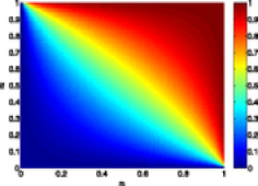
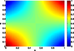
(a)	(b)

Figure 1: (a) Partial quantile indices and (b) probabilities of comparison for $x\in$ $[0,1]^{2}$ in Example 4.

indices $\tau_{x}$ and $p_{x}$ for each $x\in$ $[0,1]^{2}$. The shapes of the partial quantile surfaces can be inferred from the color bands of partial quantile indices, with each band containing $\mathcal{Q}(\tau)$ for an interval of values of $\tau$. The symmetry leads to the partial quantiles being on the diagonal, and we can see from the graph of values of $p_{x}$ on the diagonal that $p_{\tau}\rightarrow 1$ as $\tau\rightarrow 0$ or $1$ and is minimized at the partial median $x_{0.5}=(1/2,1/2)$, with $\wp=1/2$.

Since partial quantiles generalize univariate quantiles under the natural ordering, we must inherit some of its features. For example, multiplicity is possible. However, we note that in a multidimensional setting with the additional freedom of a partial order, the set of $\tau$-partial quantiles for a given $\tau$ does not need to be convex. Multiplicity and nonconvexity of the set of $\tau$-partial quantiles for a given $\tau$ are illustrated by the next example, which can be thought of as a mixture of two populations. In the univariate case, mixtures, just as any other distributions, always lead to convex collections of quantiles.

Example 5 ((Nonuniqueness)).

Consider the random variable

$$X\sim\operatorname{Uniform}\bigl{(}(-1,1)\times(1,3)\cup(1,3)\times(-1,1)\bigr{)}$$

with $a\succcurlyeq b$ only if $a\geq b$ componentwise. In this case, no points in the square $(-1,1)\times(1,3)$ can be compared with any point in the square $(1,3)\times(-1,1)$. This situation leads to nonuniqueness of the partial quantiles. For $\tau\in(0,1)$, we have

$$x_{\tau}\in\left\{\pmatrix{-1+2\tau\cr 1+2\tau},\pmatrix{1+2\tau\cr-1+2\tau}\right\}\quad\mbox{and}\quad p_{\tau}=\frac{(1-\tau)^{2}+\tau^{2}}{2}.$$

Here $\wp=1/4$ and $p_{\tau}\leq 1/2$ for every $\tau\in(0,1)$, because the two squares are not in alignment with the partial order. See Figure 2 for the representation. Moreover, the set of $\tau$-partial

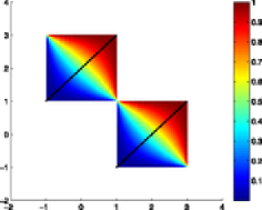
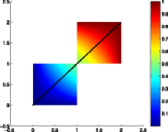
(a)	(b)

Figure 2: (a) The potential nonuniqueness of the partial quantiles arising from the partial order (Example 5). (b) The case of the partial order being aligned with the probability distribution (Example 6).

quantiles for a given $\tau$ is not convex. For example, the set of $\tau$-partial quantiles for $\tau=1/2$ is $\{(0,2)^{\prime},(2,0)^{\prime}\}$. The intuitive geometric notion of a spatial median would report the point $(1,1)^{\prime},$ which is not a partial quantile because it is not comparable with any point in the support of the distribution and thus having $p_{(1,1)}=0$.

In the next example, which also involves a mixture of two populations, the probability distribution is better aligned with the partial order.

Example 6 ((Aligned distribution and partial order)).

Consider the random variable

$$X\sim\operatorname{Uniform}([0,1]^{2}\cup[1,2]^{2})$$

with $a\succcurlyeq b$ only if $a\geq b$ componentwise. The probabilities of the events $\{X\succcurlyeq x\}$ and $\{X\preccurlyeq x\}$ are

$$P(X\succcurlyeq x) = \frac{1+(1-x_{1})(1-x_{2})}{2},$$

$$P(X\preccurlyeq x) = \frac{x_{1}x_{2}}{2}\qquad\mbox{for }x\in[0,1]^{2}$$

and

$$P(X\succcurlyeq x) = \frac{(2-x_{1})(2-x_{2})}{2},$$

$$P(X\preccurlyeq x) = \frac{1+(x_{1}-1)(x_{2}-1)}{2}\qquad\mbox{for }x\in[1,2]^{2}.$$

The partial quantiles can be computed explicitly:

$$x_{\tau} = \frac{\sqrt{1+4({1}/({2\tau})-1)}-1}{2({1}/({2\tau})-1)}\pmatrix{1\cr 1}\qquad\mbox{for }\tau<1/2,$$

$$x_{\tau} = \pmatrix{1\cr 1}\qquad\mbox{for }\tau=1/2$$

and

$$x_{\tau}=\biggl{(}2-\frac{\sqrt{1+4({1}/({2(1-\tau)})-1)}-1}{2({1}/({2(1-\tau)})-1)}\biggr{)}\pmatrix{1\cr 1}\qquad\mbox{for }\tau>1/2.$$

Note that in contrast to Example 5, we have $\wp=3/4$ in this case since the ordering is somewhat aligned with the distribution [see Figure 2(b)].

Examples 5 and 6 show the impact the alignment of the probability distribution with the partial order can have on the partial quantiles and on $p_{x_{\tau}}$. This alignment is good in Example 6, and the partial quantiles are on the main diagonal. Any point $x\in\mathcal{Q}(\tau)$ for some $\tau$ will have a lower $p_{x}$ than $x_{\tau}$, the member of $\mathcal{Q}(\tau)$ on the main diagonal. Here the maximization of the probability of drawing a comparable point leads to partial quantiles that are consistent with what we might expect. In Example 5, on the other hand, the maximization of the probability of drawing a comparable point leads to two partial quantiles for each value of $\tau$. Each of these two partial quantiles seems reasonable in the context of the square that it is in. Since the two squares are not in alignment with the partial order, however, the two $\tau$-partial quantiles for a given $\tau$ are disconnected. Results like this are to be expected with such a lack of alignment. This is analogous to trying to identify a mode with a bimodal distribution having widely separated modes.

There are extreme cases in which the probability distribution is not aligned at all with the partial order, as illustrated by Example 7.

Example 7 ((Noncomparable)).

Let $X\sim\operatorname{Uniform}(\Delta^{d-1})$, where $d>1$,

$$\Delta^{d-1}=\Biggl{\{}x\in{\mathbb{R}}^{d}\dvtx x\geq 0,\sum_{j=1}^{d}x_{j}=1\Biggr{\}}$$

is the $(d-1)$-dimensional simplex, and $a\succcurlyeq b$ only if $a\geq b$ componentwise. In this case, no two points can be compared. Therefore, we have $p_{x}=0$ and $P(X\succcurlyeq x|\mathcal{C}(x))=P(X\preccurlyeq x|\mathcal{C}(x))=1$ for all $x\in\Delta^{d-1}$. Definition 2 yields $\mathcal{Q}^{*}(\tau)=\mathcal{Q}(\tau)=\Delta^{d-1}$ for all $\tau\in(0,1)$ and $\wp=0$.

Although Example 7 might suggest a departure from the traditional quantile definition, it deals with the somewhat extreme case in which no points are comparable. This situation is in sharp contrast with the complete order that we are accustomed to in the univariate case. Nonetheless, it provides a meaningful illustration of a situation in which no point is better than any other if we rely only on the partial order. This situation is analogous to trying to compare points on a Pareto-efficient set, or an efficient frontier, where the points on the frontier dominate other points below and to the left of the frontier but the partial order does not allow us to say that any point on the efficient frontier is better than any other.

Next, we consider the case of a complete order in detail, as described earlier. Note that many complete orders are not partial orders since antisymmetry might fail. Nonetheless, all the quantities proposed here can be defined analogously.

Example 8 ((Complete order)).

Suppose that the binary relation $\preccurlyeq$ can be represented by a real-valued measurable function, that is, $x\succcurlyeq y$ if and only if $u(x)\geq u(y)$ for some $u\dvtx\mathcal{S}\rightarrow{\mathbb{R}}$. This is a well-behaved case in which we have a complete order in $\mathcal{S}$. Therefore, we have

$$P(X\succcurlyeq x_{\tau})=P\bigl{(}u(X)\geq u(x_{\tau})\bigr{)}\geq(1-\tau)\quad\mbox{and}\quad P\bigl{(}u(X)\leq u(x_{\tau})\bigr{)}\geq\tau.$$

Consider the (standard) quantile curve $q_{u(X)}\dvtx(0,1)\to\mathbb{R}$ of the random variable $u(X)$. Then $p_{x}=p_{\tau}=\wp=1$, $\tau_{x}=q_{u(X)}^{-1}(u(x))$, $\mathcal{Q}(\tau)=u^{-1}(q_{u(X)}(\tau))$ and $\mathcal{Q}^{*}(\tau)=\mathcal{Q}(\tau)$.

The situation described in Example 8 is encountered, for example, in decision analysis when the consequences in a decision-making problem are multidimensional in nature and $u$ might be represented by a payoff or utility function (e.g., Keeney and Raiffa KeeneyRaiffa1976 ). We emphasize that the reparametrization allows us to reduce to the standard univariate case, but the partial quantiles in the original space $\mathcal{S}$ would be given by the preimage of the function $u$ and could have an arbitrary geometry even if we have an interval (possibly a point) in terms of $u$.

In the following example, a random set is the random element of interest in the appropriate space under the inclusion ordering (see Molchanov Molchanov2005 for precise definitions).

Example 9 ((Interval covering)).

Let $\mathcal{S}$ be the set of all closed intervals on $[0,1]$, and let $X$ be a closed random interval,

$$X=[\xi_{1},\xi_{2}],\qquad\xi_{j}\sim\operatorname{Uniform}([0,1])\qquad\mbox{for }j=1,2.$$

The partial order is given by $a\succcurlyeq b$ only if $b\subset a$. Let $x=[x_{1},x_{2}]\subset[0,1]$ be an interval. Then we have

$$P(X\succcurlyeq x)=2x_{1}(1-x_{2})\quad\mbox{and}\quad P(X\preccurlyeq x)=|x_{2}-x_{1}|^{2},$$

which characterize the partial quantile surfaces. Using Anderson’s lemma, and letting $a(\tau)=\sqrt{2(1-\tau)/\tau}$, one can show that partial quantiles are achieved on symmetric intervals centered at $1/2$ and given by

$$x_{\tau}=\biggl{[}\frac{1}{2}-\frac{1}{2+2a(\tau)},\frac{1}{2}+\frac{1}{2+2a(\tau)}\biggr{]}$$

and

$$p_{\tau}=\biggl{(}\frac{1}{1+a(\tau)}\biggr{)}^{2}+2\biggl{(}\frac{1}{2}-\frac{1}{2+2a(\tau)}\biggr{)}^{2}.$$

Next, we consider an example of a discrete set $\mathcal{S}$.

Example 10 ((Partial order based on acyclic directed graphs)).

Let $X$ be a uniform random variable on $\mathcal{S}=\{a,b,c,d,e,f,g,h,i,j,k\}$. The partial order relation is given by an acyclic directed graph, as in Figure 3(a), and $x\preccurlyeq y$ if there is a path from $x$ to $y$ in the graph. Figure 3(b) illustrates how the partial order relation impacts the partial quantile indices and probabilities of comparison. Note also that $P(X\preccurlyeq f)\geq 0.5$ and $P(X\succcurlyeq f)\geq 0.5$, making $f$ the partial median.

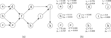
Figure 3: (a) Acyclic directed graph with $x\preccurlyeq y$ if there is a path from $x$ to $y$. (b) Displays partial quantile indices and probabilities of comparisons.

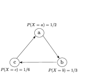
Figure 4: The cyclic directed graph with $x\preccurlyeq y$ if there is an arc from $x$ to $y$. The cycle indicates that the binary relation is not transitive. Moreover, there are no extreme partial quantiles in this example.

We conclude the examples with a binary relation that is not transitive.

Example 11 ((Nontransitive binary relation)).

Let $X$ be a random variable with values in $\mathcal{S}=\{a,b,c\}$, $P(X=a)=1/2$, $P(X=b)=1/3$ and $P(X=c)=1/6$. The binary relation is given by a directed graph, as in Figure 4, and $x\preccurlyeq y$ if there is an arc from $x$ to $y$ in the graph. The cycle in the graph indicates that the binary relation is not transitive. We note that in this particular example, there are no extreme partial quantiles. That is, the partial quantile surfaces are $\mathcal{Q}(\tau)=\varnothing$ for $\tau$ sufficiently close to $0$ or $1$.

5.1 Illustration of estimation: The unit square example

In order to illustrate previous results and statements from Sections 2, 3, 3.4 and 4, we consider Example 4 in detail. In this case, $\mathcal{S}=[0,1]^{2}$, the probability distribution $P$ is the uniform distribution on $[0,1]^{2}$, and the partial order is given by the $a\succcurlyeq b$ only if $a\geq b$ (i.e., $a_{1}\geq b_{1}$ and $a_{2}\geq b_{2}$), which is a conic order with $K={\mathbb{R}}_{+}^{2}$. For convenience, we denote the dimension of $\mathcal{S}$ be $d=2$.

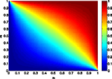
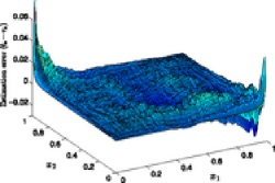
(a)	(b)

Figure 5: (a) Estimated partial quantile indices and (b) the difference between the estimated and true partial quantile indices for uniform samples on the unit square.

The class of sets $\mathcal{T}=\{\mathcal{C}(x),\{y\in\mathcal{S}\dvtx y\preccurlyeq x\},\{y\in\mathcal{S}\dvtx y\succcurlyeq x\}\dvtx x\in\mathcal{S}\}$ is a VC class of sets whose VC dimension is of the order $d$, so we have $v(\mathcal{T})\lesssim d$. We consider the metric to be the usual euclidian norm $d(x,y)=\|x-y\|$. From Theorem 8, we have $\wp=1/2^{d-1}$.

Condition E.2 holds with $v(\bar{p})\lesssim d/\bar{p}^{2}$. Condition E.3 for $\tau\in(0,1)$ holds with $\alpha=2$ and $c=1/2^{d}$ (note that for $\tau\in\{0,1\}$ we would have $\alpha=1$). Condition E.4 holds with $\gamma=2$ for $\tau=0.5$ and $\gamma=1$ otherwise. Condition E.5 holds with $\phi_{n}(r)\lesssim(r^{1/2}+n^{-1/4})\sqrt{\log n}$ by applying maximal inequalities (the $\log n$ term can be dropped if we are interested in a single quantile). Finally, condition E.6 holds by an uniform central limit theorem over $\mathcal{T}$ (see Dudley Dudley2000 , Theorem 3.7.2, or van der Vaart and Wellner vdV-W , Theorem 2.5.2).

In Figures 5 and 6, we display the estimated partial quantile indices and points for the case of $d=2$ with a sample size of $n=5\mbox{,}000$. Note that the graph of the estimated partial quantile indices in Figure 5 looks very similar to the graph of the true partial quantile indices in Figure 1. The difference between the true and estimated values is also shown in Figure 5. In light of Theorem 1, the partial quantile surface is estimated uniformly over $\mathcal{C}_{\bar{p}}$ at an $n^{1/2}$-rate of convergence if $\bar{p}$ is fixed. We see from the difference between the true and estimated values in Figure 5 that the convergence is slower at the top left and bottom right corners, which correspond to points with small probabilities of comparison $p_{x}$.

Although the exact partial quantiles fall on the $x_{1}=x_{2}$ diagonal, we can see from the few quantiles labeled in Figure 6 that they are not evenly spaced along the diagonal. Instead, they are closer together for $\tau$ near 0.5 and more spread out as $\tau\rightarrow$ 0 or 1. Moreover, the exact and estimated values of $p_{\tau}$ are smaller for $\tau$ near 0.5 (the minimum value of the exact $p_{\tau}$ is $p_{0.5}=0.5$) and grow larger as $\tau\rightarrow$ 0 or 1. The estimated quantiles in Figure 6 are close to but not equal to the true quantiles. Also, there is a slight violation of monotonicity in the estimated quantiles, a point we will expand upon later.

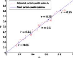
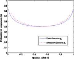
(a)	(b)

Figure 6: (a) True and estimated partial quantiles and (b) true and estimated $p_{\tau}$ as a function of $\tau$ for uniform samples on the unit square.

If we are interested in computing partial quantiles only for the case of $\mathcal{U}=\{1/2\}$, we can take $\gamma=2$, which yields a $n^{1/3}$-rate of convergence by Theorem 2. Note that for $\mathcal{U}=\{0,1\}$ we have $\gamma=1$ and $\alpha=1$, which also leads us to a $n^{1/3}$-rate of convergence by Theorem 2. On the other hand, if we are interested in computing for a nondegenerate interval $\mathcal{U}$ of quantiles, we have that $\gamma=1$, which leads to an $n^{1/4}$-rate of convergence.

Figure 7 illustrates the application of the rearrangement procedure proposed here to the estimated partial quantiles in Figure 6, which violated monotonicity for $\tau\in[0.35,0.40]$. The rearrangement results in estimated partial quantiles that coincide with the original estimates except for $\tau\in[0.35,0.40],$ where they are modified to eliminate the violation of monotonicity.

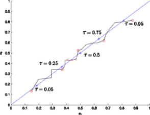
Figure 7: The componentwise rearrangement procedure applied to the estimated partial quantiles from Figure 6.

Exact and estimated dispersion regions with $\eta=g(\theta)=\theta$ for Example 4 are shown in Figure 8, corresponding to the exact and estimated partial quantile indices given in Figures 1 and 5. The

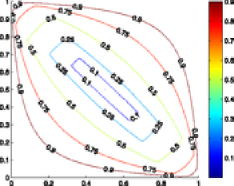
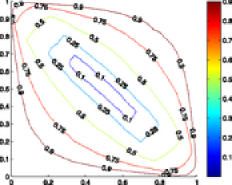
(a)	(b)

Figure 8: (a) True and (b) estimated dispersion regions $\mathcal{R}(\theta,\theta)$ for Example 4, with the boundaries of the regions labeled by $\theta$.

dispersion regions seem intuitively reasonable, and the estimated regions are quite similar to the exact regions. The dispersion regions for high values of $\theta$ extend out toward $(0,1)^{\prime}$ and $(1,0)^{\prime}$, to regions where the probabilities of comparison are low.

6 Applications

In this section, we use the concept of partial quantiles in two empirical applications, one involving the intake of dietary components and the other involving the performance of mutual funds. Our goal is not to do a detailed, full-scale analysis in each case, but to briefly illustrate the use of partial quantiles and show some of the capabilities of the concepts and measures discussed here. In particular, partial quantiles provide useful graphical and quantitative summaries of the data.

6.1 Intake nutrients within diets

Quantitative information regarding the intake distribution of several dietary components (e.g., calcium, iron, protein, Vitamin A and Vitamin C) has been collected by the U.S. Department of Agriculture (USDA) through periodic surveys. This information is used to formulate food assistance programs, consumer education efforts, and food regulatory activities. One important concept in analyzing food consumption data is the usual intake, defined as the long-run average of daily intakes of dietary components by individuals. Nusser et al. NCDF1996 propose an approach that assumes the existence of a transformation of the data such that both the original distribution and measurement errors are normally distributed. Among other relevant statistics, they estimate the quantiles of several dietary components, focusing on each component separately.

For simplicity, we consider only two dietary components, daily intakes of iron (in milligrams) and protein (in grams), in our analysis. The partial order is the componentwise natural order. Partial quantiles are relevant in this situation because not all pairs of diets (as summarized by their usual intakes) are necessarily comparable in the sense that we can say that one of the pair is “better” than the other. If one diet has more iron and the other has more protein, for example, they are not comparable. We recognize that this partial order rule may not hold for all values of the intakes. At extremely high levels of a component, it may be undesirable to increase the intake yet further, but we will assume that the partial order holds within the range of the data. Another factor that can be relevant is that intakes of different dietary components are not independent. With this partial order, for example, a positive correlation between iron intakes and protein intakes is more in alignment with the partial order and will lead to higher probabilities of comparison than a negative correlation. Therefore, understanding this dependence can be important in designing policies such as those mentioned above. Moreover, the invariance of partial quantiles under order-preserving transformations is important since different components tend to have different scales.

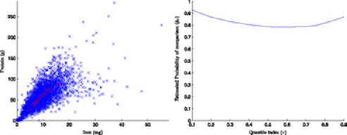
Figure 9: (a) Data (scatter diagram) and partial quantiles, and (b) estimated probabilities of comparison $\widehat{p}_{\tau}$ for the (multidimensional) iron and protein levels in food intakes.

The data we use are a subset of the data from the 1985 Continuing Survey of Food Intakes by Individuals (CSFII) USDA87 , a data source used in NCDF1996 . A scatter diagram of the data is given in Figure 9, which indicates that the data are quite well-aligned with the partial order. The estimated partial quantiles shown on this scatter diagram are monotonically increasing (in terms of the partial order) in $\tau$. We would expect to see some diets that are not comparable. Different people may tend to emphasize different types of foods, with different mixes of nutrients, in their diets. Nonetheless, the data indicate that all of the estimated partial quantiles $\widehat{x}_{\tau}$ are comparable with more than $78\%$ of the sampled diets, as can be seen from Figure 9. This suggests that partial quantiles can be interpreted very similarly to the usual univariate quantiles. For example, when deriving policies/activities/programs, the decision maker can consider the $0.5$-partial quantile to be a reasonable representation of the “median” individual. Table 2 and Figure 10 display comparisons of estimated univariate quantiles and partial quantiles. In this case, the partial quantiles are slightly more concentrated around central values than are the univariate quantiles. This reflects the intuitive notion that it is too extreme to interpret a componentwise univariate quantile as its multidimensional counterpart. We note that the univariate quantiles in Table 2 differ from those for the same nutrients in NCDF1996 because we present the standard sample quantiles, whereas a measurement error model and assumptions of normality are used to generate estimated quantiles in NCDF1996 .

Table 2: Comparison between estimated univariate quantiles and partial quantiles for iron and protein intakes

Quantile	Univariate quantile		Partial quantile
Index ($\bolds\tau$)	Iron (mg)	Protein (g)	Iron (mg)	Protein (g)
0.1	$4.51$	$25.95$	$4.69$	$25.97$
0.2	$5.99$	$35.62$	$6.16$	$37.51$
0.25	$6.61$	$39.89$	$6.74$	$41.83$
0.3	$7.12$	$43.53$	$7.33$	$44.72$
0.4	$8.11$	$49.63$	$8.21$	$50.49$
0.5	$9.12$	$56.48$	$9.09$	$59.14$
0.6	$10.29$	$63.61$	$9.97$	$62.03$
0.7	$11.47$	$70.81$	$10.85$	$67.80$
0.75	$12.30$	$75.50$	$11.44$	$73.57$
0.8	$13.25$	$80.82$	$12.61$	$76.45$
0.9	$16.30$	$95.34$	$15.84$	$87.99$

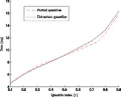
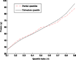
(a)	(b)

Figure 10: Estimated partial quantiles and univariate quantiles for intakes of (a) iron and (b) protein.

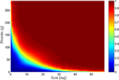
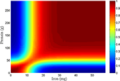
(a)	(b)

Figure 11: (a) Estimated partial quantile indices and (b) estimated probabilities of comparison for levels of iron and protein in food intakes.

Figure 11 gives more details, showing the estimated partial quantile indices $\tau_{x}$ and the probabilities of comparison $p_{x}$ for all $x$. The borders between colors indicating the partial quantile indices capture the shape of the “quality” of the diets in a comparative sense and show that the partial quantile surfaces appear convex for these data. For example, a subject with levels of iron and protein of $(17.894,87.995)$ will be on the $0.95$ partial quantile surface among diets that are comparable with her diet, since her diet is on the upper right-hand border of the light red band in Figure 11(a). This border can be thought of as a partially efficient frontier of the intake of iron and protein at a $95\%$ level in this application since any diets on that border are better than $95\%$ of the comparable diets. Moreover, this partial quantile surface allows us to consider comparative statics of the changes needed to stay at the same partial quantile level but with higher probabilities of comparison. Note that the graph of the probabilities of comparison is roughly symmetric, with $p_{x}$

ka

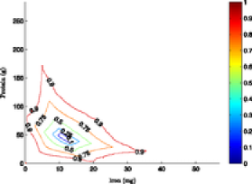
Figure 12: The dispersion measure $\mathcal{R}(\theta,\theta)$ based on estimated partial quantiles for the (multidimensional) iron and protein levels in food intakes. The boundaries of the regions are labeled by $\theta$.

decreasing as we move away from the rough “axis of symmetry” along a particular partial quantile surface. This is consistent with the location of the partial quantiles in Figure 9. Figure 12 provides yet additional information by showing the regions $\mathcal{R}(\theta,\theta)$ from the dispersion measure in (4.5) for selected values of $\theta$.

6.2 Evaluating investment funds

Next, we consider evaluating the performance of investment funds. Several indices have been considered toward this end in the Finance literature. A central approach is to regress the return of the fund ($R_{F}$) above the return on the risk free asset ($r$) against the return of the market ($R_{M}$) above the return on the risk free asset

$$(R_{F}-r)=\alpha+\beta(R_{M}-r),$$

which arises from a standard CAPM model (e.g., Sharpe1964 ). The exposure with respect to $\beta$ should not be rewarded, and higher values of the intercept $\alpha$, the risk adjusted return (i.e., the expected return on the fund when the market yields a return of zero) should be rewarded.

An emerging literature within finance advocates that in addition to the risk-adjusted return, market timing should also be rewarded (see HM1981 , JK1986 , Wermers2000 , Andrade2008 and the references therein). The difference between returns on the market and returns on the fund can be broken down by whether they are positive or negative to capture market timing Andrade2008 :

$$(R_{F}-r)=\alpha+\beta^{+}\max\{R_{M}-r,0\}+\beta^{-}\min\{R_{M}-r,0\}.$$ (22)

Note that $\max\{R_{M}-r,0\}\geq 0$ and $\min\{R_{M}-r,0\}\leq 0$; a better performance would have $\beta^{+}$ positive (the more positive the better) and $\beta^{-}$ negative (the more negative the better). Therefore, in the model (22), the quantity $\Delta:=\beta^{+}-\beta^{-}$ captures the market timing ability of the fund. Once again, the partial order that we will use for the pair $(\alpha,\Delta)$ is the componentwise natural order.

We use the data used by Andrade in Andrade2008 . Figure 13 shows the data, the estimated partial quantiles, and the associated probabilities of comparison. Since the partial order is not complete, we expect to have funds that are noncomparable. In contrast to the previous application, the data are not well-aligned with the partial order. It appears that $\alpha$ and $\Delta$ have a strong negative correlation. As a result, the estimated values for the probabilities of comparison $p_{\tau}$ are very small, always below $0.20$ and with $\widehat{\wp}=0.00651$.

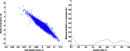
Figure 13: Data, estimated partial quantiles, and estimated probabilities of comparison for the performance of investment funds.

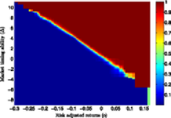
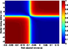
(a)	(b)

Figure 14: (a) Estimated partial quantile indices and (b) estimated probabilities of comparison for the performance of investment funds.

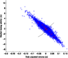
Figure 15: The componentwise rearrangement procedure applied to the estimated partial quantile points for the performance of investment funds. The difference is $2.141$.

Figure 14(a) shows that the partial quantile surfaces for different values of $\tau$ are quite close to each other and, except for extreme values of $\tau$, follow a pattern that is linear with a negative slope. This narrow band passes through a region with probabilities of comparison quite low everywhere, consistent with the above observation regarding Figure 13. Therefore, small random variation can cause potentially large shifts in partial quantile indices. As a result, the estimated partial quantiles are not monotonic. When we apply the rearrangement procedure from Section 4, we get the results shown in Figure 15. The rearranged partial quantiles are monotonic, but note that many fall outside the support of the data. Moreover, the $\ell_{2}(\mathcal{U})$ distance between the rearranged and the original estimator of the partial quantile point process is $2.141$ within the range of $\tau\in(0.1,0.9)$. These observations provide strong evidence that the true partial quantiles are not partial-monotone in the sense of (13).

How can we interpret the results for this evaluation of investment funds? We suggest that the results provide some evidence that most (if not all) of the funds may actually be optimizing their choices and (up to random fluctuation) performing on the efficient frontier. Therefore, their performance is not dominated by many other funds, and when it is, the differences in performance are slight and seem consistent with random variation. Similarly, their performance does not dominate many other firms. This lack of much domination in the data set would explain the low probabilities of comparability. Since funds have different targets for the ideal trade-off between risk and return, we should not be surprised to observe many points on or near different portions of the efficient frontier in the data, and the data seem to be consistent with this expectation. To some extent, this is very similar in spirit to Example 7, where no point is comparable with any other point.

6.3 Tobacco and health knowledge scale (THKS)

We consider the Television School and Family Smoking Prevention Cessation Project (TVSFP) study (Flay et al. Flayetal1988 and Gibbons and Hedeker GibbonsHedeker1997 ), which was designed to test the effects of a school-based social resistance classroom curriculum and a media (television) intervention program in terms of tobacco use prevention and cessation. We refer the reader to GibbonsHedeker1997 for the details of the experiment, and we report the data collected in Table 3.

=250pt Subgroup THKS score CC TV Pass Fail Total No No 175 246 0,412 (41.6) (58.6) No Yes 201 215 0,416 (48.3) (51.7) Yes No 240 140 0,380 (63.2) (36.8) Yes Yes 231 152 0,383 (60.3) (39.7) Total 847 753 1,600 (52.9) (47.1)

Table 3: Tobacco and health knowledge scale postintervention results subgroups frequencies (and percentages) GibbonsHedeker1997

The partial order of the policy maker is to obtain a “Pass” over “Fail” regardless of the subgroup. For the same result of the THKS, given cost and political considerations, it is preferred not to have used social resistance classroom curriculum (CC) or a media (television) intervention (TV). However, the subgroup with no CC and TV is not comparable to CC and no TV. The partial order is summarized by the acyclic directed graph in Figure 16.

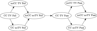
Figure 16: The partial order represented by an acyclic directed graph. We have that $a\preccurlyeq b$ if there is a directed path from $a$ to $b$.

Based on the data of Table 3 and the partial order described in Figure 16, we compute the partial quantile indices and probabilities of comparison, see Figure 17.

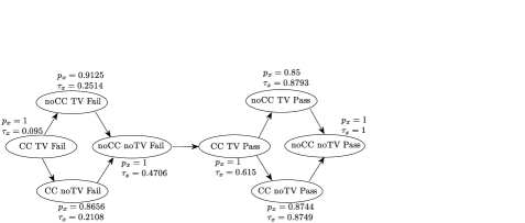
Figure 17: The figure displays partial quantile indices and probabilities of comparisons. According to the partial order of the policy maker we have $P(X\succcurlyeq\mbox{``CC TV Pass''})\geq 1/2$ and $P(X\preccurlyeq\mbox{``CC TV Pass''})\geq 1/2$ making “CC TV Pass” the (partial) median.

In this application we note the high values of the probability of comparisons. That makes the interpretation of partial quantiles very similar to traditional quantiles. In particular, the outcome “CC TV Pass” is such that $P(X\succcurlyeq\mbox{``CC TV Pass''})\geq 1/2$ and $P(X\preccurlyeq\mbox{``CC TV Pass''})\geq 1/2$ making “CC TV Pass” the (partial) median.

7 Conclusions

We propose a new generalization of quantiles to the multivariate case based on a given partial order. An important feature of our definition is that it is based only on the probability distribution and on the partial order, which might or not on the geometry of the underlying space. It leads to a concept that has several desirable properties, including robustness to outliers and equivatiance/invariance under transformations that preserve the partial order. Several issues regarding estimation and computability are investigated and discussed. In particular, rates of convergence are derived, as are asymptotic distributions of many quantities, and efficient computation is shown for an important subclass of distributions and partial orders.

The partial order is the additional structure exploited in this work. It is clear that partial quantiles depend crucially on the choice of the partial order. Therefore, their interpretation will also depend heavily on the partial order. We advocate that the choice of the partial order is application dependent. Thus, the relevance of these concepts for a particular application is linked with how meaningful the partial order is for that application. An alternative approach would be to choose the partial order to achieve partial quantiles with a desired property. For instance, one might want partial quantiles with high probabilities of comparison (which can be achieved with any binary relation that is a complete order), or partial quantiles that characterize the probability distribution (which can be achieved if the partial order induces a determining class), etc. Although these types of goals can be achieved by the appropriate choice of a partial order, it is very important for the partial order to make sense in the context of the specific application because the interpretation of all the concepts will be tied with that partial order.

Many extensions of the concept of partial quantiles are possible. For instance, the idea of embedding the partial quantile notion within a regression framework is of interest, as in Chakraborty2003 , Chaudhuri1996 , ChenGooijer2007 , HPS2009 , KB78 . Another possibility is to study the pattern of partial quantile surfaces conditional on covariates, since partial quantile surfaces also provide a meaningful generalization of the concept of an efficient frontier.

Censored models have a wide range of applications and have attracted considerable interest due to their connection with quantiles observed by Powell Powell1984 , Powell1986a , Powell1986b , Powell1991 and others NeweyPowell1990 , Portnoy2003 , NBP2006 , BuchinskyHahn1998 , Womersley1986 . However, typical data exhibit censoring in more than one variable. Due to the equivariance under order-preserving transformations, the proposed generalization of quantiles is suitable to be applied to censored multidimensional data.

Moreover, another motivation to consider partial orders, or more general preferences, is the connection with the literature of decision theory. For example, the identification of axioms on the preferences that allow for statistical inference, computational tractability, etc., is of interest. Similarly, the identification of classes of decision problems for which partial quantiles play an important role in optimal strategies would be very valuable. Although the pursuit of these extensions is outside the scope of this paper, we believe that they provide questions of interest for future research.

Appendix A Section 2 proofs

Proof of Proposition 1 This follows from the equivalence between the events $\{h(X)\succcurlyeq h(Y)\}$ and $\{X\succcurlyeq Y\}$, and the events $\{h(X)\succ h(Y)\}$ and $\{X\succ Y\}$. Proof of Proposition 2 If $m$ is an invariance mapping, it follows that $\mathcal{C}(m(x))=m(\mathcal{C}(x))$ and $X\succcurlyeq m(x)=m(X\succcurlyeq x)$. Therefore,

$$P\bigl{(}X\succcurlyeq m(x)|\mathcal{C}(m(x))\bigr{)} = \frac{P(X\succcurlyeq m(x))}{P(\mathcal{C}(m(x)))}=\frac{P(m(X\succcurlyeq x))}{P(m(\mathcal{C}(x)))}$$

$$= \frac{P(X\succcurlyeq x)}{P(\mathcal{C}(x))}=P\bigl{(}X\succcurlyeq x|\mathcal{C}(x)\bigr{)}.$$

This implies that if $x\in\mathcal{Q}(\tau)$, then $m(x)\in\mathcal{Q}(\tau)$, and if $x$ is a $\tau$-partial quantile, so is $m(x)$. Proof of Proposition 3 Since the binary relation is transitive, $\{X\succ x\}\subseteq\{X\succ x^{\prime}\}$ and $\{X\preccurlyeq x\}\supseteq\{X\preccurlyeq x^{\prime}\}$, so that $P(X\succ x^{\prime})\geq P(X\succ x)\geq 0$ and $P(X\preccurlyeq x)\geq P(X\preccurlyeq x^{\prime})\geq 0$. Therefore,

$$\tau_{x} = P\bigl{(}X\preccurlyeq x|\mathcal{C}(x)\bigr{)}$$

$$= \frac{P(X\preccurlyeq x)}{P(X\preccurlyeq x)+P(X\succ x)}\geq\frac{P(X\preccurlyeq x^{\prime})}{P(X\preccurlyeq x^{\prime})+P(X\succ x)}$$

$$\geq \frac{P(X\preccurlyeq x^{\prime})}{P(X\preccurlyeq x^{\prime})+P(X\succ x^{\prime})}=\tau_{x^{\prime}}.$$

Appendix B Section 3 proofs

Proof of Lemma 1 We can assume that $X$ has a compact support to ensure that integrals are well defined (and standard approximation arguments yields the full result, or we are establishing probabilistic bounds and the compact set is chosen to control the probability).

Since $K$ is a convex set, the associated class of functions $\mathcal{T}$ is measurable and $\partial K$ has zero Lebesgue measure by Lemma 2.4.3 in Dudley Dudley2000 . Moreover, $\mathcal{T}$ is a VC class of sets with VC index at most $3d+4$. Therefore, condition E.2 holds with $v(\bar{p})=(3d+4)/\bar{p}^{2}$.

Let $\sigma_{0}$ denote the surface measure on $\partial K$. To establish E.5, let

$$\mu:=\sup_{x\in\mathbb{R}^{d}}\int_{\partial(-K\cup K)}f(x+y)\,d\sigma_{0}(y)<\infty,$$

since the support of $X$ is compact. Next, note that $d(x,y)=\|x-y\|\geq E[|1\{X\in\mathcal{C}(x)\}-1\{X\in\mathcal{C}(y)\}|^{2}]/\mu$. Then E.5 holds with $\phi_{n}(r)\lesssim(\sqrt{\mu r}+n^{-1/4})\sqrt{\log n}$ by Theorem 2.14.17 of van der Vaart and Wellner vdV-W . If $\mathcal{U}$ is a singleton, we can improve the bound to $\phi_{n}(r)\lesssim\sqrt{\mu r}+n^{-1/4}$ using arguments in Kim and Pollard KimPollard1990 .

Since $\mathcal{T}$ is a VC class and $K$ is a convex set which ensures enough measurability, E.6 holds by Theorem of 2.6.8 in van der Vaart and Wellner vdV-W .

To establish E.3, building upon Section 5 in Kim and Pollard KimPollard1990 , note that

$$\nabla\tau_{x} = \frac{1}{p_{x}}\int_{\partial(-K)}f(x+y)n_{(-K)}(y)\,d\sigma_{0}(y)$$

$${}-\frac{\tau_{x}}{p_{x}}\int_{\partial(-K\cup K)}f(x+y)n_{(-K\cup K)}(y)\,d\sigma_{0}(y)$$

and

$$\nabla^{2}p_{x}=\int_{\partial(-K\cup K)}\nabla f(x+y)n_{(-K\cup K)}(y)^{\prime}\,d\sigma_{0}(y),$$

where $n_{A}(y)$ is the outward pointing unit vector normal to $\partial A$ at $y$. Letting $B_{1}=\partial(-K\cup K)\cap\partial(-K)$, $B_{2}=\partial(-K\cup K)\setminus\partial(-K)\subset\partial K$, we have

$$p_{x}\nabla\tau_{x} = \int_{\partial(-K)\setminus B_{1}}f(x+y)n_{(-K)}(y)\,d\sigma_{0}(y)$$

$${}+(1-\tau_{x})\int_{B_{1}}f(x+y)n_{(-K)}(y)\,d\sigma_{0}(y)$$

$${}-\tau_{x}\int_{B_{2}}f(x+y)n_{(-K\cup K)}(y)\,d\sigma_{0}(y)$$

$$= \int_{\partial(-K)}\bigl{(}1\{y\in B_{1}^{c}\}+(1-\tau_{x})1\{y\in B_{1}\}+\tau_{x}1\{y\in-B_{2}\}\bigr{)}$$

$$\hskip 28.1pt{}\times f(x+y)n_{(-K)}(y)\,d\sigma_{0}(y).$$

Since $-K$ is a convex cone with nonempty interior, the normal vectors cannot be (positively) linearly dependent. Therefore, we have $\nabla\tau_{x}\neq 0$ for any $x$ in the interior of the support of the random variable $X$. Therefore, $\mathcal{Q}(\tau)=\tau_{x}^{-1}(\tau)$ is a continuously differentiable hypersurface for every $\tau\in(0,1)$ by the Global Implicit Function theorem. The smoothness of $p_{x}$ and $\mathcal{Q}(\tau)$ yields condition E.3 with $\alpha=2$ for all $\tau\in\mathcal{U}$.

Also, $p_{x}=\int_{-K\cup K}f(x+y)\,dy$ and $\tau_{x}=(1/p_{x})\int_{-K}f(x+y)\,dy$ are twice differentiable functions. Therefore, $p_{\tau}$ is Lipschitz for $\tau\in\mathcal{U}$ since $\mathcal{U}\subset(0,1)$ is compact and $\wp>0$ under our conditions. Thus, condition E.4(i) is satisfied with $\gamma=1$. Moreover, continuity of $p_{x}$ and $\tau_{x}$ also implies that the mapping $\mathcal{Q}^{*}(\tau)$ is upper-semi continuous. Proof of Lemma 2 The bound on E.2 follows from the union bound. Condition E.3 follows from the finite cardinality of $\mathcal{S}$ since for $x\in\mathcal{Q}(\tau)\setminus\mathcal{Q}^{*}(\tau)$ we have $p_{x}<p_{\tau}$ and for $x\in\mathcal{Q}^{\ast}(\tau)$ we have $p_{x}=p_{\tau}$. Take $c=\min_{\tau\in\mathcal{U}}p_{\tau}-\max_{x\in\mathcal{Q}(\tau)\setminus\mathcal{Q}^{*}(\tau)}p_{x}>0$ since $\mathcal{U}$ is compact. Condition E.5 follows similarly to E.2, noting that for $d(x,y)<1$ we have $x=y$. Condition E.6 follows trivially. Finally, E.4 follows by noting that $p_{\tau}$ and $x_{\tau}$ are piecewise constant mappings with a finite number of jumps. Thus, if $\mathcal{U}$ does not include the indices corresponding to these jumps, E.4 holds trivially. Proof of Theorem 1 For convenience, let $W_{x}=\{X\preccurlyeq x\}$. Then, for all $x\in\mathcal{S}$ such that $p_{x}\geq\bar{p}$ we have, by condition E.2,

$$|\widehat{\tau}_{x}-\tau_{x}| = \biggl{|}\frac{\mathbb{P}_{n}(W_{x})-P(W_{x})}{p_{x}}+\mathbb{P}_{n}(W_{x})\biggl{(}\frac{1}{\widehat{p}_{x}}-\frac{1}{p_{x}}\biggr{)}\biggr{|}$$

$$= \biggl{|}\frac{\mathbb{P}_{n}(W_{x})-P(W_{x})}{p_{x}}+\widehat{\tau}_{x}\biggl{(}\frac{p_{x}-\widehat{p}_{x}}{p_{x}}\biggr{)}\biggr{|}$$

$$\leq \biggl{|}\frac{\mathbb{P}_{n}(W_{x})-P(W_{x})}{p_{x}}\biggr{|}+\widehat{\tau}_{x}\biggl{|}\frac{p_{x}-\widehat{p}_{x}}{p_{x}}\biggr{|}$$

$$\lesssim \!\mbox{${}_{P}$\,}\sqrt{v(\bar{p})/n}.$$

Lemma 8 ((Technical lemma)).

Let $0<\epsilon_{1}\vee\epsilon_{2}<\epsilon_{3}<1/2$ and $f,g,h\dvtx\break[0,1]\to[0,1]$, such that for all $t\in[0,1]$,

$$\limsup_{t^{k}\to t}f(t^{k}) \leq f(t)+\epsilon_{1},\qquad\limsup_{t^{k}\to t}g(t^{k})\leq g(t)+\epsilon_{1}\quad\mbox{and}$$

$$\liminf_{t^{k}\to t}h(t^{k}) \geq h(t)-\epsilon_{1}.$$

Moreover, assume that $\epsilon_{2}<\epsilon_{3}\min_{t\in[0,1]}h(t)$, and for every $t\in[\epsilon_{3},1-\epsilon_{3}]$:

$|f(t)-th(t)|\leq\epsilon_{2}$,

$|g(t)-(1-t)h(t)|\leq\epsilon_{2}$ and

$f(t)+g(t)\geq h(t)$. Then, for every $\tau\in(3\epsilon_{3},1-3\varepsilon_{3})$ there is $\bar{t}$ such that $f(\bar{t})\geq\tau h(\bar{t})-2\epsilon_{1}$ and $g(\bar{t})\geq(1-\tau)h(\bar{t})-2\epsilon_{1}$.

Let $\bar{t}=\sup_{t\in[\epsilon_{3},1-\epsilon_{3}]}t\dvtx g(t)\geq(1-\tau)h(t)$. We have that $g(2\epsilon_{3})\geq(1-2\epsilon_{3})h(2\epsilon_{3})-\epsilon_{2}=(1-\tau)h(2\epsilon_{3})+(\tau-2\epsilon_{3})h(2\epsilon_{3})-\epsilon_{2}\geq(1-\tau)h(2\epsilon_{3})$ by the assumption on $\epsilon_{2}$ and $\tau$. Similarly, $g(1-2\epsilon_{3})\leq 2\epsilon_{3}h(1-2\epsilon_{3})-\epsilon_{2}<(1-\tau)h(2\epsilon_{3})$. So $\bar{t}\in[2\epsilon_{3},1-2\epsilon_{3}]$.

Moreover, the condition (8) on $g$ and $h$ implies that $g(\bar{t})\geq(1-\tau)h(\bar{t})-2\epsilon_{1}$ and, by the definition of $\bar{t}$, $g(\bar{t}+\mu)<(1-\tau)h(\bar{t}+\mu)$ for every $\mu>0$. Thus, $f(\bar{t}+\mu)>\tau h(\bar{t}+\mu)$ for every $\mu>0$ by (iii). In turn, condition (8) for $f$ and $h$ yields $f(\bar{t})\geq\tau h(\bar{t})-2\epsilon_{1}$, which establishes the result. Proof of Theorem 2 The proof proceeds in steps. Step 1 establishes feasibility of a “near” partial quantile point. Step 2 derives the main arguments. Step 3 concludes the proof.

Step 1. Feasibility of near partial quantile point. Note that for any point $x$ that is feasible for (3.3) we have $|\tau-\widehat{\tau}_{x}|\leq\epsilon_{n}/\widehat{p}_{x}$. Moreover, by Theorem 1, if also $p_{x}\geq\wp$, we have $|\widehat{\tau}_{x}-\tau_{x}|\lesssim_{P}\sqrt{v(\wp)/n}$, so that $|\tau-\tau_{x}|\lesssim_{P}u_{n}:=\sqrt{v(\wp)/n}+\epsilon_{n}/\wp$.

Assume that $\epsilon_{n}\geq\epsilon_{n}^{D}$. Pick an arbitrary $x_{\tau}\in\mathcal{Q}^{*}(\tau)$. By condition E.4, there is a continuous path of quantile points, $\mathcal{P}=\{x_{\tau^{\prime}}\dvtx\tau^{\prime}\in(0,1)\}$, that passes through $x_{\tau}$. Let $\epsilon_{1}=\epsilon_{n}/2$, $\epsilon_{2}=\sqrt{v(\wp)/n}$ and $\epsilon_{3}=(1/6)\min_{u\in\mathcal{U}}u\wedge(1-u)$, so that $f(t)=\mathbb{P}_{n}(X\preccurlyeq x_{t})$, $g(t)=\mathbb{P}_{n}(X\succcurlyeq x_{t})$, and $h(t)=\widehat{p}_{x_{t}}$ satisfies condition (8), (i) and (ii) by Theorem 1 and (iii) by definition. By Lemma 8, there exists $x_{\tau^{*}}\in\mathcal{P}$ that is feasible for (3.3). Since $p_{\tau^{*}}\geq\wp$, we have $|\tau-\tau^{*}|\lesssim_{P}u_{n}$. On the other hand, if $\epsilon_{n}\geq\epsilon_{n}^{D^{\prime}}$, $x_{\tau}\in\mathcal{Q}^{*}(\tau)$ is itself feasible with high probability. We can take $x_{\tau^{*}}=x_{\tau}$ and the relation $|\tau-\tau^{*}|\lesssim_{P}u_{n}$ would still hold.

Step 2. Main argument. We will derive the rate of convergence by bounding

$$p_{\tau_{\widehat{x}_{\tau}}}-p_{\widehat{x}_{\tau}}=p_{\tau_{\widehat{x}_{\tau}}}-p_{\tau}+p_{x_{\tau}}-p_{\widehat{x}_{\tau}}$$

from above using E.5 and the optimality of $\widehat{x}_{\tau}$, and from below using the restricted identification condition E.2.

To establish the upper bound first note that by optimality of $\widehat{x}_{\tau}$, we have $\widehat{p}_{x_{\tau^{*}}}\leq\widehat{p}_{\widehat{x}_{\tau}}$ and using E.5,

$$p_{x_{\tau}}-p_{\widehat{x}_{\tau}} \lesssim_{P} \phi_{n}(d(\widehat{x}_{\tau},x_{\tau}))/\sqrt{n}+\widehat{p}_{x_{\tau}}-\widehat{p}_{\widehat{x}_{\tau}}$$

$$\lesssim_{P} \phi_{n}(d(\widehat{x}_{\tau},x_{\tau}))/\sqrt{n}+\widehat{p}_{x_{\tau}}-\widehat{p}_{x_{\tau^{*}}}.$$

Applying E.5 one more time, and using that $|\tau^{*}-\tau|\lesssim_{P}u_{n}$ so that $d(x_{\tau^{*}},\break x_{\tau})\lesssim_{P}u_{n}$ and $p_{x_{\tau}}-p_{x_{\tau^{*}}}\lesssim_{P}u_{n}^{\gamma}$,

$$p_{x_{\tau}}-p_{\widehat{x}_{\tau}} \lesssim_{P} \phi_{n}(d(\widehat{x}_{\tau},x_{\tau}))/\sqrt{n}+\phi_{n}(d(x_{\tau},x_{\tau^{*}}))/\sqrt{n}+p_{x_{\tau}}-p_{x_{\tau^{*}}}$$

$$\lesssim_{P} \phi_{n}(d(\widehat{x}_{\tau},x_{\tau}))/\sqrt{n}+\phi_{n}(u_{n})/\sqrt{n}+u_{n}^{\gamma}.$$

Also, since $|\tau_{\widehat{x}_{\tau}}-\tau|\lesssim_{P}u_{n}$, by E.4, $p_{\tau_{\widehat{x}_{\tau}}}-p_{\tau}\lesssim_{P}u_{n}^{\gamma}$.

Note that if $d(\widehat{x}_{\tau},x_{\tau})\lesssim_{P}u_{n}^{\gamma}$ we are done. Therefore, the relations above yields

$$p_{\tau_{\widehat{x}_{\tau}}}-p_{\widehat{x}_{\tau}}\lesssim_{P}\phi_{n}(d(\widehat{x}_{\tau},x_{\tau}))/\sqrt{n}+u_{n}^{\gamma}.$$

By E.3, we can minorate the left-hand side and obtain

$$c\wedge\inf_{z\in\mathcal{Q}^{*}(\tau_{\widehat{x}_{\tau}})}d(\widehat{x}_{\tau},z)^{\alpha}\lesssim_{P}\phi_{n}(d(\widehat{x}_{\tau},x_{\tau}))/\sqrt{n}+u_{n}^{\gamma}.$$

Since the argument holds for all $x_{\tau}\in\mathcal{Q}^{*}(\tau)$, we have

$$c\wedge\inf_{z\in\mathcal{Q}^{*}(\tau_{\widehat{x}_{\tau}})}d(\widehat{x}_{\tau},z)^{\alpha}\lesssim_{P}\phi_{n}\Bigl{(}\inf_{x_{\tau}\in\mathcal{Q}^{*}(\tau)}d(\widehat{x}_{\tau},x_{\tau})\Bigr{)}\big{/}\sqrt{n}+u_{n}^{\gamma}.$$

Next note that the minimum in the left-hand side cannot be $c$ as $n$ grows [since $\phi_{n}(d(\widehat{x}_{\tau},x_{\tau}))$ can be bounded by $2\sqrt{v(\wp/2)}=o(n^{1/2})$ by Theorem 1].

Step 3. Conclusion of the proof. Using that $\alpha\geq 1$ by E.3, E.4(ii), and the last relation in Step 2,

$$\inf_{x_{\tau}\in\mathcal{Q}^{*}(\tau)}d(\widehat{x}_{\tau},x_{\tau})$$

$$\qquad\leq\inf_{x_{\tau}\in\mathcal{Q}^{*}(\tau),z\in\mathcal{Q}^{*}(\tau_{\widehat{x}_{\tau}})}d(\widehat{x}_{\tau},z)+d(z,x_{\tau})$$

$$\qquad\lesssim\inf_{z\in\mathcal{Q}^{*}(\tau_{\widehat{x}_{\tau}})}d(\widehat{x}_{\tau},z)+|\tau-\tau_{\widehat{x}_{\tau}}|$$

$$\qquad\lesssim_{P}\phi_{n}^{1/\alpha}\Bigl{(}\inf_{x_{\tau}\in\mathcal{Q}^{*}(\tau)}d(\widehat{x}_{\tau},x_{\tau})\Bigr{)}\big{/}n^{1/2\alpha}+u_{n}^{\gamma/\alpha}+u_{n}$$

$$\qquad\lesssim_{P}u_{n}\vee u_{n}^{\gamma/\alpha}\vee\phi_{n}^{1/\alpha}\Bigl{(}\inf_{x_{\tau}\in\mathcal{Q}^{*}(\tau)}d(\widehat{x}_{\tau},x_{\tau})\Bigr{)}\big{/}n^{1/2\alpha}.$$

The rate result follows as in vdV-W . Proof of Corollary 1 Since the order is complete, $p_{x}=\widehat{p}_{x}=1$ for every $x\in\mathcal{S}$. In particular, condition E.5 is satisfied with $\phi_{n}(r)=0$, E.4 with $\gamma=\alpha$ and E.3 with any positive $\alpha$ since $\mathcal{Q}^{*}(\tau)=\mathcal{Q}(\tau)$. In this case $\epsilon_{n}:=\epsilon_{n}^{D}\wedge\epsilon_{n}^{D^{\prime}}\leq\epsilon_{n}^{D^{\prime}}\lesssim_{P}\sqrt{v(1)/n}$. Proof of Theorem 3 For convenience, let $\mathcal{W}_{x}=\{X\preccurlyeq x\}$ and $\mathcal{C}_{x}=\mathcal{C}(x)$. By E.6 we have $\sqrt{n}(\mathbb{P}_{n}(\mathcal{W}_{x})-P(\mathcal{W}_{x}))\rightsquigarrow N(0,P(\mathcal{W}_{x})(1-P(\mathcal{W}_{x})))$ and $\sqrt{n}(\widehat{p}_{x}-p_{x})\rightsquigarrow N(0,p_{x}(1-p_{x}))$.

Moreover, we have

$$\widehat{\tau}_{x}-\tau_{x} = \frac{\mathbb{P}_{n}(\mathcal{W}_{x})}{\widehat{p}_{x}}-\frac{P(\mathcal{W}_{x})}{p_{x}}=\frac{\mathbb{P}_{n}(\mathcal{W}_{x})}{\widehat{p}_{x}}-\frac{\mathbb{P}_{n}(\mathcal{W}_{x})}{p_{x}}+\frac{\mathbb{P}_{n}(\mathcal{W}_{x})-P(\mathcal{W}_{x})}{p_{x}}$$

$$= \mathbb{P}_{n}(\mathcal{W}_{x})\biggl{(}\frac{1}{\widehat{p}_{x}}-\frac{1}{p_{x}}\biggr{)}+\frac{\mathbb{P}_{n}(\mathcal{W}_{x})-P(\mathcal{W}_{x})}{p_{x}}$$

$$= \frac{\mathbb{P}_{n}(\mathcal{W}_{x})}{\widehat{p}_{x}}\frac{p_{x}-\widehat{p}_{x}}{p_{x}}+\frac{\mathbb{P}_{n}(\mathcal{W}_{x})-P(\mathcal{W}_{x})}{p_{x}}$$

$$= -\widehat{\tau}_{x}\frac{\widehat{p}_{x}-p_{x}}{p_{x}}+\frac{\mathbb{P}_{n}(\mathcal{W}_{x})-P(\mathcal{W}_{x})}{p_{x}}$$

$$= (\tau_{x}-\widehat{\tau}_{x})\frac{\widehat{p}_{x}-p_{x}}{p_{x}}-\tau_{x}\frac{\widehat{p}_{x}-p_{x}}{p_{x}}+\frac{\mathbb{P}_{n}(\mathcal{W}_{x})-P(\mathcal{W}_{x})}{p_{x}}.$$

By Condition E.2, $|\frac{\widehat{p}_{x}-p_{x}}{p_{x}}|\lesssim_{P}\sqrt{v(\bar{p})/n}=o_{P}(1)$, so that

$$\bigl{(}1+o_{P}(1)\bigr{)}p_{x}(\widehat{\tau}_{x}-\tau_{x}) = -\tau_{x}(\widehat{p}_{x}-p_{x})+\mathbb{P}_{n}(\mathcal{W}_{x})-P(\mathcal{W}_{x})$$

$$= \frac{1}{\sqrt{n}}\mathbb{G}_{n}(1\{\mathcal{W}_{x}\}-\tau_{x}1\{\mathcal{C}_{x}\}).$$

Therefore, we have $p_{x}\sqrt{n}(\widehat{\tau}_{x}-\tau_{x})=_{P}\mathbb{G}_{n}(1\{\mathcal{W}_{x}\}-\tau_{x}1\{\mathcal{C}_{x}\}).$ That converges to a zero mean normal distribution with variance

$$\mathbf{E}[(1\{\mathcal{W}_{x}\}-\tau_{x}1\{\mathcal{C}_{x}\})^{2}] = P(\mathcal{W}_{x})+\tau_{x}^{2}p_{x}-2\tau_{x}P(\mathcal{W}_{x})$$

$$= P(\mathcal{W}_{x})(1-\tau_{x})+\tau_{x}\bigl{(}\tau_{x}p_{x}-P(\mathcal{W}_{x})\bigr{)}$$

$$= P(\mathcal{W}_{x})(1-\tau_{x})$$

using $\mathcal{W}_{x}\subseteq\mathcal{C}_{x}$ and $\tau_{x}=P(\mathcal{W}_{x})/p_{x}$. Finally, we get

$$\sqrt{n}(\widehat{\tau}_{x}-\tau_{x})\rightsquigarrow N\biggl{(}0,\frac{\tau_{x}(1-\tau_{x})}{p_{x}}\biggr{)}.$$

Note that within $\mathcal{C}_{\bar{p}}$, all the functions are bounded by $2/\bar{p}$ with high probability for large enough sample size. Therefore, a multidimensional central limit theorem applies and the covariance structure of a pair $x,y\in\mathcal{S}$ is given by

$$\Omega_{x,y}=\mathbf{E}\biggl{[}\frac{(1\{\mathcal{W}_{x}\}-\tau_{x}1\{\mathcal{C}_{x}\})}{p_{x}}\frac{(1\{\mathcal{W}_{y}\}-\tau_{y}1\{\mathcal{C}_{y}\})}{p_{y}}\biggr{]}.$$

After simplification, we obtain

$$\Omega_{x,y} = \frac{P(\mathcal{W}_{x}\cap\mathcal{W}_{y})}{P(\mathcal{C}_{x})P(\mathcal{C}_{y})}-\tau_{x}\frac{P(\mathcal{C}_{x}\cap\mathcal{W}_{y})}{P(\mathcal{C}_{x})P(\mathcal{C}_{y})}-\tau_{y}\frac{P(\mathcal{C}_{y}\cap\mathcal{W}_{x})}{P(\mathcal{C}_{x})P(\mathcal{C}_{y})}+\tau_{x}\tau_{y}\frac{P(\mathcal{C}_{x}\cap\mathcal{C}_{y})}{P(\mathcal{C}_{x})P(\mathcal{C}_{y})}$$

$$= \tau_{x}\tau_{y}\biggl{(}\frac{P(\mathcal{W}_{x}\cap\mathcal{W}_{y})}{P(\mathcal{W}_{x})P(\mathcal{W}_{y})}-\frac{P(\mathcal{C}_{x}\cap\mathcal{W}_{y})}{p_{x}P(\mathcal{W}_{y})}-\frac{P(\mathcal{W}_{x}\cap\mathcal{C}_{y})}{P(\mathcal{W}_{x})p_{y}}+\frac{P(\mathcal{C}_{x}\cap\mathcal{C}_{y})}{p_{x}p_{y}}\biggr{)}.$$

Finally, asymptotic equicontinuity of $\beta_{n}(x)$ follows directly from the asymptotic equicontinuity of $\alpha_{n}(x)$ implied by E.6 and $\bar{p}>0$ being fixed. Proof of Corollary 2 The proof of the second result builds upon arguments in EinmahlMason1992 , BucchianicoEinmahlMushkudiani2001 . Based on Theorem 3, we have that for $\mathcal{C}_{\wp/2}=\{x\in\mathcal{S},p_{x}\geq\wp/2\}$, the process $\beta_{n}(x):=\sqrt{n}(\widehat{\tau}_{x}-\tau_{x})$ converges weakly in $\ell^{\infty}(\mathcal{C}_{\wp/2})$ to a bounded, mean zero Gaussian process $G_{P}$. By the Skorohod–Dudley–Wichura representation theorem, there exists a probability space $(\widetilde{\Omega},\mathcal{\widetilde{A}},\widetilde{P})$ carrying versions $\widetilde{G}_{P}$ and $\widetilde{\beta}_{n}$ of $G_{P}$ and $\beta_{n}$ such that $\sup_{x\in\mathcal{C}_{\wp/2}}|\widetilde{\beta}_{n}(x)-\widetilde{G}_{P}(x)|\to 0$ as $n$ grows. Next, note that for all $\tau\in\mathcal{U}$, $\widehat{x}_{\tau}\in\mathcal{C}_{\wp/2}$ provided that $\sqrt{v(\wp)/n}=o(\wp)$. Thus,

$$\sqrt{n}(\tau_{\widehat{x}_{\tau}}-\tau)=-\widetilde{\beta}_{n}(\widehat{x}_{\tau})+\sqrt{n}(\widehat{\tau}_{\widehat{x}_{\tau}}-\tau)=o(1)+\widetilde{G}_{P}(\widehat{x}_{\tau})+\sqrt{n}(\widehat{\tau}_{\widehat{x}_{\tau}}-\tau).\quad$$

Proof of Theorem 4 Let $\tau^{*}$ and $\widehat{\tau}^{*}$ be such that $\wp=p_{\tau^{*}}$ and $\widehat{\wp}=\widehat{p}_{\widehat{\tau}^{*}}$. Thus, we have $\widehat{x}_{\widehat{\tau}^{*}}$ and $\widehat{x}_{\tau^{*}}$ satisfying $\widehat{p}_{\widehat{\tau}^{*}}=\widehat{p}_{\widehat{x}_{\widehat{\tau}^{*}}}$ and $\widehat{p}_{\tau^{*}}=\widehat{p}_{\widehat{x}_{\tau^{*}}}$. Moreover, let $u_{n}:=\sqrt{v(\wp)/n}+\epsilon_{n}/\wp\lesssim n^{-1/2}$ by assumption.

First, note that since $\widehat{\wp}\leq\widehat{p}_{\tau^{*}}$, and $p_{\tau_{\widehat{x}_{\tau^{*}}}}\geq p_{\widehat{x}_{\tau^{*}}}$, we have, by E.5,

$$\widehat{\wp}-\wp \leq \widehat{p}_{\tau^{*}}-p_{\tau^{*}}=\widehat{p}_{\widehat{x}_{\tau^{*}}}-p_{x_{\tau^{*}}}$$

$$= \widehat{p}_{\widehat{x}_{\tau^{*}}}-p_{\widehat{x}_{\tau^{*}}}-(\widehat{p}_{x_{\tau^{*}}}-p_{x_{\tau^{*}}})+p_{\widehat{x}_{\tau^{*}}}-p_{x_{\tau^{*}}}+\widehat{p}_{x_{\tau^{*}}}-p_{x_{\tau^{*}}}$$

$$\lesssim \!\mbox{${}_{P}$\,}\phi_{n}(d(\widehat{x}_{\tau^{*}},x_{\tau^{*}}))/\sqrt{n}+p_{\tau_{\widehat{x}_{\tau^{*}}}}-p_{x_{\tau^{*}}}+\widehat{p}_{x_{\tau^{*}}}-p_{x_{\tau^{*}}}.$$

Note also that by Step 1 in the proof of Theorem 2 we have $|\tau_{\widehat{x}_{\tau^{*}}}-\tau^{*}|\lesssim_{P}u_{n}$. Moreover, $p_{\tau}$ is locally quadratic around $\tau^{*}$. Therefore,

$$\widehat{\wp}-\wp\lesssim_{P}\phi_{n}(d(\widehat{x}_{\tau^{*}},x_{\tau^{*}}))/\sqrt{n}+u_{n}^{2}+\widehat{p}_{x_{\tau^{*}}}-p_{x_{\tau^{*}}}.$$

Since it holds for any $x_{\tau^{*}}\in\mathcal{Q}^{*}(\tau^{*})$,

$$\widehat{\wp}-\wp \lesssim_{P} \phi_{n}\Bigl{(}\inf_{x_{\tau^{*}}\in\mathcal{Q}^{*}(\tau^{*})}d(\widehat{x}_{\tau^{*}},x_{\tau^{*}})\Bigr{)}\big{/}\sqrt{n}$$

$${}+u_{n}+\max_{x_{\tau^{*}}\in\mathcal{Q}^{*}(\tau^{*})}\{\widehat{p}_{x_{\tau^{*}}}-p_{x_{\tau^{*}}}\}$$

$$\lesssim_{P} o(n^{-1/2})+\max_{x_{\tau^{*}}\in\mathcal{Q}^{*}(\tau^{*})}\{\widehat{p}_{x_{\tau^{*}}}-p_{x_{\tau^{*}}}\}$$

since $u_{n}^{2}=o(n^{-1/2})$, and $\inf_{x_{\tau^{*}}\in\mathcal{Q}^{*}(\tau^{*})}d(\widehat{x}_{\tau^{*}},x_{\tau^{*}})=o_{P}(1)$ by Theorem 2.

Next, by Step 1 in the proof of Theorem 2, for every $x_{\widehat{\tau}^{*}}$ there is a partial quantile point $x_{\bar{\tau}}$, $d(x_{\widehat{\tau}^{*}},x_{\bar{\tau}})\lesssim u_{n}$ that is feasible for (3.3) with $\widehat{\tau}^{*}$. Thus, $\widehat{p}_{\widehat{x}_{\widehat{\tau}^{*}}}\geq\widehat{p}_{x_{\bar{\tau}}}$. Using this inequality, E.5, and that $p_{\widehat{\tau}^{*}}\geq p_{\tau^{*}}$ by definition (4),

$$\widehat{\wp}-\wp \geq \widehat{p}_{x_{\bar{\tau}}}-p_{x_{\tau^{*}}}$$

$$= \widehat{p}_{x_{\bar{\tau}}}-p_{x_{\bar{\tau}}}-(\widehat{p}_{x_{\tau^{*}}}-p_{x_{\tau^{*}}})+p_{x_{\bar{\tau}}}-p_{x_{\tau^{*}}}+\widehat{p}_{x_{\tau^{*}}}-p_{x_{\tau^{*}}}$$

$$\gtrsim \!\mbox{${}_{P}$\,}-\phi_{n}(d(x_{\bar{\tau}},x_{\tau^{*}}))/\sqrt{n}+p_{x_{\widehat{\tau}^{*}}}-p_{x_{\tau^{*}}}+\widehat{p}_{x_{\tau^{*}}}-p_{x_{\tau^{*}}}$$

$$\geq -\phi_{n}(d(x_{\bar{\tau}},x_{\tau^{*}}))/\sqrt{n}+\widehat{p}_{x_{\tau^{*}}}-p_{x_{\tau^{*}}},$$

where $x_{\bar{\tau}}$ was chosen to be close to $x_{\tau^{*}}$, namely $d(x_{\bar{\tau}},x_{\tau^{*}})\leq d(x_{\bar{\tau}},x_{\widehat{\tau}^{*}})+d(x_{\widehat{\tau}^{*}},x_{\tau^{*}})\lesssim_{P}u_{n}+|\widehat{\tau}^{*}-\tau^{*}|$. Therefore, (B) holds for any $x_{\tau^{*}}\in\mathcal{Q}^{*}(\tau^{*})$ and $d(x_{\widehat{\tau}^{*}},x_{\tau^{*}})\lesssim|\widehat{\tau}^{*}-\tau^{*}|=o_{P}(1)$ by Lemma 9 below. Thus,

$$\widehat{\wp}-\wp\geq-o_{P}(n^{-1/2})+\max_{x_{\tau^{*}}\in\mathcal{Q}^{*}(\tau^{*})}\{\widehat{p}_{x_{\tau^{*}}}-p_{x_{\tau^{*}}}\}.$$ (26)

Combining (26) and (B), we obtain $\sqrt{n}(\widehat{\wp}-\wp)=o_{P}(1)+Z_{P}(\tau^{*})$.

Lemma 9.

Under the assumptions of Theorem 2, and that $\tau\mapsto p_{\tau}$ is a twice differentiable function, let $\wp=p_{\tau^{*}}$ and $\widehat{\wp}=\widehat{p}_{\widehat{\tau}^{*}}$. Then $|\widehat{\tau}^{*}-\tau^{*}|=o_{P}(1)$.

Consider the twice differentiable function $\tau\mapsto p_{\tau}$. Since $p_{\tau^{*}}$ is its strict minimum at the interior of $\mathcal{U}$, we have $p_{\tau}-p_{\tau^{*}}\gtrsim|\tau-\tau^{*}|^{2}$ for $\tau\in\mathcal{U}$.

By Step 1 of the proof of Theorem 2, for every $\tau\in\mathcal{U}$ we have that there is an $x_{\bar{\tau}}$ that is feasible and $|\bar{\tau}-\tau|\lesssim_{P}u_{n}=o_{P}(1)$. Thus,

$$\widehat{p}_{\tau}=\widehat{p}_{\widehat{x}_{\tau}}\geq\widehat{p}_{x_{\bar{\tau}}}\gtrsim_{P}p_{\bar{\tau}}-\sqrt{v(\wp)/n}\gtrsim_{P}p_{\tau}-\sqrt{v(\wp)/n}-u_{n}^{\gamma}=o_{P}(1)+p_{\tau}.$$

Similarly, since $|\tau_{x_{\bar{\tau}}}-\tau|\lesssim_{P}u_{n}$,

$$\widehat{p}_{\tau} \lesssim_{P} p_{\widehat{x}_{\tau}}+\sqrt{v(\wp/2)/n}\lesssim_{P}p_{\tau_{x_{\bar{\tau}}}}+\sqrt{v(\wp/2)/n}$$

$$\lesssim_{P} p_{\tau}+\sqrt{v(\wp/2)/n}+u_{n}^{\gamma}=o_{P}(1)+p_{\tau}.$$

Therefore, using that $\widehat{p}_{\widehat{\tau}^{*}}\leq\widehat{p}_{\tau^{*}}$,

$$|\widehat{\tau}-\tau^{*}|^{2}\leq p_{\widehat{\tau}^{*}}-p_{\tau^{*}}=o_{P}(1)+v-\widehat{p}_{\tau^{*}}=o_{P}(1).$$

Appendix C Section 4 proofs

Proof of Lemma 4 This follows if $\operatorname{support}\widehat{1}_{K}=\mathbb{R}^{d}$, where $\widehat{1}_{K}$ is the Fourier transform of the indicator function of the set $K$, see BagchiSitaram1982 , Proposition 3.1. (We proceed as in Proposition 3.2 in BagchiSitaram1982 with the necessary modifications.)

Step 1. Let $0\neq f\in L^{1}(\mathbb{R}^{d})$ such that $\operatorname{support}f\subseteq K$, $\widehat{f}(w)=\int_{\mathbb{R}^{d}}e^{-iw^{\prime}x}\times f(x)\,dx=\int_{K}e^{-iw^{\prime}x}f(x)\,dx$, and $K^{o}=\{y\in\mathbb{R}^{d}\dvtx y^{\prime}x\leq 0$ for all $x\in K\}$ denote the polar cone of $K$. Define the regions (in the complex space $\mathbb{C}^{d}$)

$$H=\{z\in\mathbb{C}^{d}\dvtx\operatorname{Im}(z)\in K^{o}\}\quad\mbox{and}\quad H_{0}=\{z\in\mathbb{C}^{d}\dvtx\operatorname{Im}(z)\in\operatorname{int}K^{o}\}.$$

It follows from the definition that $\widehat{f}$ can be extended to a bounded function $g$ in the region $H$ [because $K$ is a proper convex cone, for any $w\in H_{0}$ and $x\in K$, we have $\operatorname{Re}(-iw^{\prime}x)\leq 0$]. Moreover, $g$ is analytic in $H_{0}$ and continuous in $H$. Therefore, $\widehat{f}$ is the restriction of the bounded analytic function $g$ on the boundary of $H$ Bochner1937 . Consequently, $\widehat{f}$ cannot be identically zero on an open subset of $\mathbb{R}^{d}$ (which would imply that $\widehat{f}=0$ and, thus, $f=0$), equivalently, $\operatorname{support}\widehat{f}=\mathbb{R}^{d}$.

Step 2. Next, we consider $1_{K}$ which is a nonzero bounded Borel function which is not in $L^{1}(\mathbb{R}^{d})$. By contradiction, assume that $\widehat{1}_{K}$ vanishes on a nonempty open set $U$ of $\mathbb{R}^{d}$, that is, $(\operatorname{support}\widehat{1}_{K})\cap U=\varnothing$. Let $x_{0}$ and $\varepsilon>0$ such that $B(x_{0},2\varepsilon)\subset U$.

Let $0\neq h_{1}\in L^{1}(\mathbb{R}^{d})$ such that $\widehat{h}_{1}$ is a $C^{\infty}$ function and $\operatorname{support}\widehat{h}_{1}\subset B(0,\varepsilon)$. Then

$$\mathrm{support}\widehat{(h_{1}\cdot 1_{K})}=\operatorname{support}(\widehat{h}_{1}*\widehat{1}_{K})\subseteq\operatorname{support}\widehat{h}_{1}+\operatorname{support}\widehat{1}_{K}\subset\mathbb{R}^{d}\setminus B(x_{0},\varepsilon),$$

where “$*$” denotes the convolution operator.

On the other hand, $h_{1}\cdot 1_{K}\in L^{1}(\mathbb{R}^{d})$ with $\operatorname{support}(h_{1}\cdot 1_{K})\subset K$. Therefore, by Step 1, $h_{1}\cdot 1_{K}=0$ almost everywhere on $\mathbb{R}^{d}$. In turn, $\widehat{h}_{1}$ is a $C^{\infty}$-function of compact support, so $h_{1}$ is the restriction of an entire function to $\mathbb{R}^{d}$, and hence $h_{1}(x)\neq 0$ almost everywhere in $\mathbb{R}^{d}$. Thus, $1_{K}$ is zero almost everywhere which give us a contradiction since $K$ is a proper convex cone. Proof of Lemma 5 Without loss of generality, we can consider only connected graphs (otherwise we proceed with each connected component separately). We provide an algorithm.

For each node, we have $\tau_{x}p_{x}=P(X\preccurlyeq x)$. If there is no incoming arc on $x$, we have that $P(X\preccurlyeq x)=P(X=x)$. For a general node $x$, if we already computed $P(X=y)$ for all $y\neq x$, $y\preccurlyeq x$, then we have $P(X=x)=\tau_{x}p_{x}-\sum_{y\neq x,y\preccurlyeq x}P(X=y)$. Otherwise, “backtrack” to consider a $y\neq x$, $y\preccurlyeq x$ for which $P(X=y)$ is not known. Since there are no cycles, we can only “backtrack” at most $|\mathcal{S}|<\infty$ before computing a probability for some $y$. Thus the procedure terminates in a finite number of steps with all probabilities. Proof of Theorem 7 The proof follows from the inequality of Lorentz Lorentz1953 applied to each component individually. This follows the strategy of Chernozhukov, Fernández-Val and Galichon CFG2009 that previously used this inequality to prove a similar result. Proof of Corollary 3 If $x_{\tau}$ is partial-monotone, by Theorem 7 we have

$$\biggl{|}\int_{0}^{1}\|\widehat{x}^{r}_{u}-\widehat{x}_{u}\|^{\kappa}\,du\biggr{|}^{1/\kappa} \leq \biggl{|}\int_{0}^{1}\|\widehat{x}_{u}^{r}-x_{u}\|^{\kappa}\,du\biggr{|}^{1/\kappa}+\biggl{|}\int_{0}^{1}\|\widehat{x}_{u}-x_{u}\|^{\kappa}\,du\biggr{|}^{1/\kappa}$$

$$\leq 2\biggl{|}\int_{0}^{1}\|\widehat{x}_{u}-x_{u}\|^{\kappa}\,du\biggr{|}^{1/\kappa}.$$

The second follows by a triangular inequality. Proof of Theorem 8 Note that by independence and no point mass, we have $P(X\succcurlyeq x)=\prod_{j=1}^{d}(1-F_{j}(x_{j}))$, $P(X\preccurlyeq x)=\prod_{j=1}^{d}F_{j}(x_{j})$ and $p_{x}=P(X\succcurlyeq x)+P(X\preccurlyeq x)$. Thus, $x_{\tau}\in\arg\max\{\prod_{j=1}^{d}(1-F_{j}(x_{j}))+\prod_{j=1}^{d}F_{j}(x_{j})\dvtx\break\tau\prod_{j=1}^{d}(1-F_{j}(x_{j}))=(1-\tau)\prod_{j=1}^{d}F_{j}(x_{j})\}$. By the independence, we can write $a_{j}=F_{j}(x_{j})$ and recast the problem as $\max_{a}\{\prod_{j=1}^{d}a_{j}+\prod_{j=1}^{d}(1-a_{j})\dvtx(1-\tau)\prod_{j=1}^{d}a_{j}=(1-\tau)\prod_{j=1}^{d}(1-a_{j}),0\leq a_{j}\leq 1\}$. By inspection, we have that $0<a_{j}<1$, $j=1,\ldots,d$, at the optimal. By the optimality conditions, there is a $\lambda$ such that we have for every $k=1,\ldots,d$

$$0=\prod_{j\neq k}a_{j}-\prod_{j\neq k}(1-a_{j})-\lambda(1-\tau)\prod_{j\neq k}a_{j}+\lambda\tau\prod_{j\neq k}(1-a_{j}).$$

This implies that for every $j=1,\ldots,d$, we have $\frac{1-\lambda\tau}{1-\lambda(1-\tau)}=\frac{\tau}{1-\tau}\cdot\frac{1-a_{k}}{a_{k}}$.

Therefore, $a_{k}^{*}=a(\tau)$ for every $k=1,\ldots,d$. On the other hand, by feasibility we must have $\prod_{j=1}^{d}[a_{j}^{*}/(1-a_{j}^{*})]=a(\tau)^{d}/(1-a(\tau))^{d}=\tau/(1-\tau)$. Therefore, $a(\tau)/(1-a(\tau))=(\tau/(1-\tau))^{1/d}$, which yields the result. Proof of Theorem 9 By Proposition 1 with $h(x)=(F_{1}(x_{1}),F_{2}(x_{2}),\ldots,\break F_{d}(x_{d}))$, we have $\tau_{X}=\tau_{h(X)}$ so that we can assume that $X$ is a uniform $(0,1)$ random variable. Therefore,

$$P(\tau_{X}\leq\tau)=P\Biggl{(}\prod_{j=1}^{d}x_{j}\leq\tau\Biggl{[}\prod_{j=1}^{d}x_{j}+\prod_{j=1}^{d}(1-x_{j})\Biggr{]}\Biggr{)}=P\Biggl{(}\prod_{j=1}^{d}\frac{x_{j}}{1-x_{j}}\leq\frac{\tau}{1-\tau}\Biggr{)}.$$

The first result follows by taking logs and noting that $Z_{j}:=\log(x_{j}/(1-x_{j}))$ is distributed as a logistic random variable with zero mean and variance $\pi^{2}/3$ when $x_{j}$ is a uniform $(0,1)$ random variable.

Next, since $Z_{j}$ is symmetric around zero, $P(\tau_{X}\geq 1/2)=P(\sum_{j=1}^{d}Z_{j}\geq 0)=1/2$. Finally, let $Z^{(d)}:=d^{-1/2}\sum_{j=1}^{d}Z_{j}$ and denote its probability density function by $f_{d}$. It follows that $\max_{z}f_{d}(z)=f_{d}(0)\leq 1/2$. Since $Z^{(d)}$ is symmetric, we have, for $t\in(0,1/2)$,

$$P(|\tau_{X}-0.5|\geq t)=2P(\tau_{X}\geq 0.5+t)=2P\biggl{(}Z^{(d)}\geq d^{-1/2}\log\biggl{(}\frac{0.5+t}{0.5-t}\biggr{)}\biggr{)}.$$

Thus, using that $\log(1+x)\leq x$ and $f_{d}(z)\leq 1/2$,

$$P(|\tau_{X}-0.5|\geq t) \geq 2P\biggl{(}Z^{(d)}\geq\frac{2td^{-1/2}}{0.5-t}\biggr{)}\geq 1-2\int_{0}^{2td^{-1/2}/(0.5-t)}f_{d}(z)\,dz$$

$$\geq 1-\frac{2td^{-1/2}}{0.5-t}.$$

Using $t:=0.5-Cd^{-1/2}$ in the expression above,

$$P(|\tau_{X}-0.5|\geq 0.5-Cd^{-1/2})\geq 1-\frac{2(0.5-Cd^{-1/2})d^{-1/2}}{Cd^{-1/2}}\geq 1-1/C.\quad$$

Proof of Lemma 6 We can compute the partial order and the probabilities $P(X\succcurlyeq x|\mathcal{C}(x))$ and $P(X\preccurlyeq x|\mathcal{C}(x))$, which are bounded by $O(|\mathcal{S}|)$ for every fixed $x\in\mathcal{S}$. Varying over all choices of $|\mathcal{S}|$, we obtain $O(|\mathcal{S}|^{2})$ operations. Proof of Lemma 7 First, note that under C.2, we have that $K$ is a convex cone with nonempty interior. Therefore, $K$ has a strict recession direction, that is, $\exists w\neq 0$ such that $K+w\subset\operatorname{int}K$. Moreover, if $K\cap-K$ is full dimensional, $K=\mathbb{R}^{d}$ and we have $x\succcurlyeq y$ for every $x,y\in\mathbb{R}^{d}$ and the result holds trivially. Therefore, we can assume that $K\cap-K$ is not full dimensional.

Since $K\cap-K$ is not full dimensional and $X$ has no point mass, we have $P(X\succcurlyeq x\succcurlyeq X)=0$ for every $x\in\mathcal{S}$. Therefore $p_{x}=P(X\succcurlyeq x)+P(X\preccurlyeq x)$. Moreover, $p_{x}$, $P(X\preccurlyeq x)$ and $P(X\succcurlyeq x)$ are continuous in $x$.

Note that any pair $(p,x)$ such that $x\in\mathcal{Q}(\tau)$ and $p=p_{x}$ is feasible for problem (7). By the log-concavity of the probability density function, $P(X\preccurlyeq x)=P(x-K)$ and $P(X\succcurlyeq x)=P(x+K)$ are log-concave functions of $x$ by the Prékopa–Leindler inequality (e.g., see Gadner2002 ). This shows that (7) can be recast as a convex programming problem.

Next, we will show that the solution to (7) also solves (3). If $p^{\ast}=p_{x^{\ast}}$, then both constraints are active at the optimal point, and the result follows. Note that at least one constraint must be active at $(p^{\ast},x^{\ast})$.

Suppose $p^{\ast}<p_{x^{\ast}}$, in which case $x^{\ast}\notin\mathcal{Q}(\tau)$. Without loss of generality, assume that $P(X\succcurlyeq x^{*})>(1-\tau)p^{\ast}$. Define the continuous functions $u(t)=P(X\succcurlyeq x^{\ast}+td)$ and $\ell(t)=P(X\preccurlyeq x^{\ast}+td)$, which are, respectively, decreasing and increasing in $t$. For some $t>0$, we have $u(t)>(1-\tau)p^{\ast}$ and $\ell(t)>\tau p^{\ast}$, which contradicts the optimality of $(p^{\ast},x^{\ast})$. Proof of Theorem 10 From Lemma 7, it follows that we can recast the problem as the convex programming problem defined in (7). For $\bar{p}<p_{\tau}$, define the convex set

$$H(\bar{p}) := \{(v,x)\in\mathbb{R}\times\mathcal{S}:\log P(X\succcurlyeq x)\geq\log(1-\tau)+v,$$

$$\hskip 39.5pt\log P(X\preccurlyeq x)\geq\log\tau+v,\log\bar{p}\leq v\leq 0\},$$

where $v=\log p$ for $p$ in (7). For an arbitrary $\varepsilon>0$, note that for every $x$ we can approximate $P(X\succcurlyeq x)$ and $P(X\preccurlyeq x)$ up to a multiplicative factor of $1+\varepsilon$ using the integration procedure for log-concave distributions based on random walks proposed by Lovász and Vempala LV2006 . Relying on these results, we can construct and $\varepsilon_{0}$-approximate a membership oracle whose complexity is given by

$$O\biggl{(}\frac{d^{4}\log^{3}d\log(1/\delta)}{\varepsilon_{0}^{2}}\biggr{)},$$

where $\varepsilon_{0}=p_{\tau}\varepsilon$. Note that by controlling the error in the computation of $P(X\preccurlyeq x)$ and $P(X\succcurlyeq x)$ by a factor of $1+\varepsilon$, we control the error in the computation of $\tau_{x}$ by an additive error of $\varepsilon$.

Based on this membership oracle, we can apply the results in LV2006 for optimization, which requires $O^{\ast}(d^{4.5})$ calls of the constructed membership oracle.

References

- (1) {barticle}[mr] \bauthor\bsnmAlexander, \bfnmKenneth S.\binitsK. S. (\byear1987). \btitleRates of growth and sample moduli for weighted empirical processes indexed by sets. \bjournalProbab. Theory Related Fields \bvolume75 \bpages379–423. \biddoi=10.1007/BF00318708, mr=0890285 \endbibitem
- (2) {barticle}[mr] \bauthor\bsnmBagchi, \bfnmS. C.\binitsS. C. and \bauthor\bsnmSitaram, \bfnmA.\binitsA. (\byear1982). \btitleDetermining sets for measures on . \bjournalIllinois J. Math. \bvolume26 \bpages419–422. \bidmr=0658452 \endbibitem
- (3) {barticle}[mr] \bauthor\bsnmBarnett, \bfnmV.\binitsV. (\byear1976). \btitleThe ordering of multivariate data. \bjournalJ. Roy. Statist. Soc. Ser. A \bvolume139 \bpages318–355. \bidmr=0445726 \endbibitem
- (4) {bbook}[mr] \bauthor\bsnmBlum, \bfnmLenore\binitsL., \bauthor\bsnmCucker, \bfnmFelipe\binitsF., \bauthor\bsnmShub, \bfnmMichael\binitsM. and \bauthor\bsnmSmale, \bfnmSteve\binitsS. (\byear1998). \btitleComplexity and Real Computation. \bpublisherSpringer, \baddressNew York. \bidmr=1479636 \endbibitem
- (5) {barticle}[mr] \bauthor\bsnmBochner, \bfnmS.\binitsS. (\byear1937). \btitleBounded analytic functions in several variables and multiple Laplace integrals. \bjournalAmer. J. Math. \bvolume59 \bpages732–738. \biddoi=10.2307/2371340, mr=1507275 \endbibitem
- (6) {barticle}[mr] \bauthor\bsnmBuchinsky, \bfnmMoshe\binitsM. and \bauthor\bsnmHahn, \bfnmJinyong\binitsJ. (\byear1998). \btitleAn alternative estimator for the censored quantile regression model. \bjournalEconometrica \bvolume66 \bpages653–671. \biddoi=10.2307/2998578, mr=1627038 \endbibitem
- (7) {barticle}[mr] \bauthor\bsnmChakraborty, \bfnmBiman\binitsB. (\byear2003). \btitleOn multivariate quantile regression. \bjournalJ. Statist. Plann. Inference \bvolume110 \bpages109–132. \biddoi=10.1016/S0378-3758(01)00277-4, mr=1944636 \endbibitem
- (8) {barticle}[mr] \bauthor\bsnmChaudhuri, \bfnmProbal\binitsP. (\byear1996). \btitleOn a geometric notion of quantiles for multivariate data. \bjournalJ. Amer. Statist. Assoc. \bvolume91 \bpages862–872. \bidmr=1395753 \endbibitem
- (9) {barticle}[mr] \bauthor\bsnmCheng, \bfnmYebin\binitsY. and \bauthor\bsnmDe Gooijer, \bfnmJan G.\binitsJ. G. (\byear2007). \btitleOn the th geometric conditional quantile. \bjournalJ. Statist. Plann. Inference \bvolume137 \bpages1914–1930. \biddoi=10.1016/j.jspi.2006.02.014, mr=2323873 \endbibitem
- (10) {barticle}[auto:STB—2010-11-18—09:18:59] \bauthor\bsnmChernozhukov, \bfnmV.\binitsV., \bauthor\bsnmFernández-Val, \bfnmI.\binitsI. and \bauthor\bsnmGalichon, \bfnmA.\binitsA. (\byear2009). \btitleImproving point and interval estimators of monotone functions by rearrangement. \bjournalBiometrika \bvolume96 \bpages559–575. \endbibitem
- (11) {barticle}[mr] \bauthor\bsnmChernozhukov, \bfnmVictor\binitsV., \bauthor\bsnmFernández-Val, \bfnmIván\binitsI. and \bauthor\bsnmGalichon, \bfnmAlfred\binitsA. (\byear2010). \btitleQuantile and probability curves without crossing. \bjournalEconometrica \bvolume78 \bpages1093–1125. \biddoi=10.3982/ECTA7880, mr=2667913 \endbibitem
- (12) {barticle}[mr] \bauthor\bsnmChernozhukov, \bfnmVictor\binitsV., \bauthor\bsnmHong, \bfnmHan\binitsH. and \bauthor\bsnmTamer, \bfnmElie\binitsE. (\byear2007). \btitleEstimation and confidence regions for parameter sets in econometric models. \bjournalEconometrica \bvolume75 \bpages1243–1284. \biddoi=10.1111/j.1468-0262.2007.00794.x, mr=2347346 \endbibitem
- (13) {bmisc}[auto:STB—2010-11-18—09:18:59] \bauthor\bparticlede \bsnmAndrade Jr., \bfnmF.\binitsF. (\byear2011). \bhowpublishedMeasures of downside risk and mutual fund flows. Kellogg School of Management, Northwestern Univ. Unpublished manuscript. \endbibitem
- (14) {barticle}[mr] \bauthor\bsnmDette, \bfnmHolger\binitsH. and \bauthor\bsnmVolgushev, \bfnmStanislav\binitsS. (\byear2008). \btitleNon-crossing non-parametric estimates of quantile curves. \bjournalJ. R. Stat. Soc. Ser. B Stat. Methodol. \bvolume70 \bpages609–627. \biddoi=10.1111/j.1467-9868.2008.00651.x, issn=1369-7412, mr=2420417 \endbibitem
- (15) {barticle}[mr] \bauthor\bsnmDi Bucchianico, \bfnmAlessandro\binitsA., \bauthor\bsnmEinmahl, \bfnmJohn H. J.\binitsJ. H. J. and \bauthor\bsnmMushkudiani, \bfnmNino A.\binitsN. A. (\byear2001). \btitleSmallest nonparametric tolerance regions. \bjournalAnn. Statist. \bvolume29 \bpages1320–1343. \biddoi=10.1214/aos/1013203456, mr=1873333 \endbibitem
- (16) {bbook}[mr] \bauthor\bsnmDudley, \bfnmR. M.\binitsR. M. (\byear1999). \btitleUniform Central Limit Theorems. \bseriesCambridge Studies in Advanced Mathematics \bvolume63. \bpublisherCambridge Univ. Press, \baddressCambridge. \biddoi=10.1017/CBO9780511665622, mr=1720712 \endbibitem
- (17) {bbook}[mr] \bauthor\bsnmDudley, \bfnmR. M.\binitsR. M. (\byear2002). \btitleReal Analysis and Probability. \bseriesCambridge Studies in Advanced Mathematics \bvolume74. \bpublisherCambridge Univ. Press, \baddressCambridge. \bidmr=1932358 \endbibitem
- (18) {barticle}[mr] \bauthor\bsnmEinmahl, \bfnmJohn H. J.\binitsJ. H. J. and \bauthor\bsnmMason, \bfnmDavid M.\binitsD. M. (\byear1992). \btitleGeneralized quantile processes. \bjournalAnn. Statist. \bvolume20 \bpages1062–1078. \biddoi=10.1214/aos/1176348670, mr=1165606 \endbibitem
- (19) {barticle}[auto:STB—2010-11-18—09:18:59] \bauthor\bsnmFlay, \bfnmB.\binitsB., \bauthor\bsnmBrannon, \bfnmB.\binitsB., \bauthor\bsnmJohnson, \bfnmC.\binitsC., \bauthor\bsnmHansen, \bfnmW.\binitsW., \bauthor\bsnmUlene, \bfnmA.\binitsA., \bauthor\bsnmWhitney-Saltiel, \bfnmD.\binitsD., \bauthor\bsnmGleason, \bfnmL.\binitsL., \bauthor\bsnmSussman, \bfnmS.\binitsS., \bauthor\bsnmGavin, \bfnmM.\binitsM., \bauthor\bsnmKimarie, \bfnmG.\binitsG., \bauthor\bsnmSobol, \bfnmD.\binitsD. and \bauthor\bsnmSpiegel, \bfnmD.\binitsD. (\byear1988). \btitleThe television school and family smoking prevention and cessation project: I. Theoretical basis and program development. \bjournalPreventive Medicine \bvolume17 \bpages585–607. \endbibitem
- (20) {barticle}[mr] \bauthor\bsnmGardner, \bfnmR. J.\binitsR. J. (\byear2002). \btitleThe Brunn–Minkowski inequality. \bjournalBull. Amer. Math. Soc. (N.S.) \bvolume39 \bpages355–405. \biddoi=10.1090/S0273-0979-02-00941-2, mr=1898210 \endbibitem
- (21) {barticle}[auto:STB—2010-11-18—09:18:59] \bauthor\bsnmGibbons, \bfnmR. D.\binitsR. D. and \bauthor\bsnmHedeker, \bfnmD.\binitsD. (\byear1997). \btitleRandom effects probit and logistic regression models for three-level data. \bjournalBiometrics \bvolume53 \bpages1527–1537. \endbibitem
- (22) {barticle}[mr] \bauthor\bsnmGiné, \bfnmEvarist\binitsE. and \bauthor\bsnmKoltchinskii, \bfnmVladimir\binitsV. (\byear2006). \btitleConcentration inequalities and asymptotic results for ratio type empirical processes. \bjournalAnn. Probab. \bvolume34 \bpages1143–1216. \biddoi=10.1214/009117906000000070, mr=2243881 \endbibitem
- (23) {bincollection}[mr] \bauthor\bsnmGrötschel, \bfnmM.\binitsM., \bauthor\bsnmLovász, \bfnmL.\binitsL. and \bauthor\bsnmSchrijver, \bfnmA.\binitsA. (\byear1984). \btitleGeometric methods in combinatorial optimization. In \bbooktitleProgress in Combinatorial Optimization (Waterloo, Ont., 1982) \bpages167–183. \bpublisherAcademic Press, \baddressToronto, ON. \bidmr=0771876 \endbibitem
- (24) {barticle}[mr] \bauthor\bsnmHallin, \bfnmMarc\binitsM., \bauthor\bsnmPaindaveine, \bfnmDavy\binitsD. and \bauthor\bsnmŠiman, \bfnmMiroslav\binitsM. (\byear2010). \btitleMultivariate quantiles and multiple-output regression quantiles: From optimization to halfspace depth. \bjournalAnn. Statist. \bvolume38 \bpages635–669. \biddoi=10.1214/09-AOS723, mr=2604670 \endbibitem
- (25) {barticle}[auto:STB—2010-11-18—09:18:59] \bauthor\bsnmHallin, \bfnmM.\binitsM., \bauthor\bsnmPaindaveine, \bfnmD.\binitsD. and \bauthor\bsnmSiman, \bfnmM.\binitsM. (\byear2010). \btitleRejoinder. \bjournalAnn. Statist. \bvolume38 \bpages694–703. \endbibitem
- (26) {barticle}[auto:STB—2010-11-18—09:18:59] \bauthor\bsnmHenriksson, \bfnmR.\binitsR. and \bauthor\bsnmMerton, \bfnmR.\binitsR. (\byear1981). \btitleOn market timing and investment performance. II. Statistical procedures for evaluating forecasting skills. \bjournalJ. Bus. \bvolume54 \bpages513–533. \endbibitem
- (27) {barticle}[mr] \bauthor\bsnmHuber, \bfnmPeter J.\binitsP. J. (\byear1973). \btitleRobust regression: Asymptotics, conjectures and Monte Carlo. \bjournalAnn. Statist. \bvolume1 \bpages799–821. \bidmr=0356373 \endbibitem
- (28) {barticle}[auto:STB—2010-11-18—09:18:59] \bauthor\bsnmJagannathan, \bfnmR.\binitsR. and \bauthor\bsnmKorajczyk, \bfnmR.\binitsR. (\byear1986). \btitleAssesing the market timing performance of managed portfolios. \bjournalJ. Bus. \bvolume59 \bpages217–235. \endbibitem
- (29) {barticle}[mr] \bauthor\bsnmKalai, \bfnmAdam Tauman\binitsA. T. and \bauthor\bsnmVempala, \bfnmSantosh\binitsS. (\byear2006). \btitleSimulated annealing for convex optimization. \bjournalMath. Oper. Res. \bvolume31 \bpages253–266. \biddoi=10.1287/moor.1060.0194, mr=2233996 \endbibitem
- (30) {bbook}[mr] \bauthor\bsnmKeeney, \bfnmRalph L.\binitsR. L. and \bauthor\bsnmRaiffa, \bfnmHoward\binitsH. (\byear1976). \btitleDecisions with Multiple Objectives: Preferences and Value Tradeoffs. \bpublisherWiley, \baddressNew York. \bidmr=0449476 \endbibitem
- (31) {barticle}[mr] \bauthor\bsnmKim, \bfnmJeanKyung\binitsJ. and \bauthor\bsnmPollard, \bfnmDavid\binitsD. (\byear1990). \btitleCube root asymptotics. \bjournalAnn. Statist. \bvolume18 \bpages191–219. \biddoi=10.1214/aos/1176347498, mr=1041391 \endbibitem
- (32) {bbook}[mr] \bauthor\bsnmKoenker, \bfnmRoger\binitsR. (\byear2005). \btitleQuantile Regression. \bseriesEconometric Society Monographs \bvolume38. \bpublisherCambridge Univ. Press, \baddressCambridge. \biddoi=10.1017/CBO9780511754098, mr=2268657 \endbibitem
- (33) {barticle}[mr] \bauthor\bsnmKoenker, \bfnmRoger\binitsR. and \bauthor\bsnmBassett, \bfnmGilbert\binitsG. Jr. (\byear1978). \btitleRegression quantiles. \bjournalEconometrica \bvolume46 \bpages33–50. \bidmr=0474644 \endbibitem
- (34) {barticle}[auto:STB—2010-11-18—09:18:59] \bauthor\bsnmKong, \bfnmL.\binitsL. and \bauthor\bsnmMizera, \bfnmI.\binitsI. (\byear2010). \btitleDiscussion of “Multivariate quantiles and multiple-output regression quantiles: From optimization to halfspace depth,” by M. Hallin, D. Paindaveine and M. Šiman. \bjournalAnn. Statist. \bvolume38 \bpages685–693. \endbibitem
- (35) {barticle}[mr] \bauthor\bsnmLorentz, \bfnmG. G.\binitsG. G. (\byear1953). \btitleAn inequality for rearrangements. \bjournalAmer. Math. Monthly \bvolume60 \bpages176–179. \bidmr=0052476 \endbibitem
- (36) {bincollection}[auto:STB—2010-11-18—09:18:59] \bauthor\bsnmLovász, \bfnmL.\binitsL. and \bauthor\bsnmVempala, \bfnmS.\binitsS. (\byear2006). \btitleFast algorithms for logconcave functions: Sampling, rounding, integration and optimization. In \bbooktitleProceedings of the 47th Annual IEEE Symposium on Foundations of Computer Science (FOCS) \bpages57–68. \bpublisherIEEE Computer Society, \baddressLos Alamitos, CA. \endbibitem
- (37) {bbook}[mr] \bauthor\bsnmMolchanov, \bfnmI. S.\binitsI. S. (\byear2005). \btitleTheory of Random Sets. \bpublisherSpringer, \baddressLondon. \endbibitem
- (38) {bbook}[mr] \bauthor\bsnmMotwani, \bfnmRajeev\binitsR. and \bauthor\bsnmRaghavan, \bfnmPrabhakar\binitsP. (\byear1995). \btitleRandomized Algorithms. \bpublisherCambridge Univ. Press, \baddressCambridge. \bidmr=1344451 \endbibitem
- (39) {barticle}[mr] \bauthor\bsnmNeocleous, \bfnmTereza\binitsT. and \bauthor\bsnmPortnoy, \bfnmStephen\binitsS. (\byear2008). \btitleOn monotonicity of regression quantile functions. \bjournalStatist. Probab. Lett. \bvolume78 \bpages1226–1229. \biddoi=10.1016/j.spl.2007.11.024, mr=2441467 \endbibitem
- (40) {barticle}[mr] \bauthor\bsnmNeocleous, \bfnmTereza\binitsT., \bauthor\bparticleVan den \bsnmBranden, \bfnmKarlien\binitsK. and \bauthor\bsnmPortnoy, \bfnmStephen\binitsS. (\byear2006). \btitleCorrection to “Censored regression quantiles,” by S. Portnoy. \bjournalJ. Amer. Statist. Assoc. \bvolume101 \bpages860–861. \biddoi=10.1198/016214506000000087, mr=2281250 \endbibitem
- (41) {barticle}[mr] \bauthor\bsnmNewey, \bfnmWhitney K.\binitsW. K. and \bauthor\bsnmPowell, \bfnmJames L.\binitsJ. L. (\byear1990). \btitleEfficient estimation of linear and type censored regression models under conditional quantile restrictions. \bjournalEconometric Theory \bvolume6 \bpages295–317. \biddoi=10.1017/S0266466600005284, mr=1085576 \endbibitem
- (42) {barticle}[auto:STB—2010-11-18—09:18:59] \bauthor\bsnmNusser, \bfnmS. M.\binitsS. M., \bauthor\bsnmCarriquiry, \bfnmA. L.\binitsA. L., \bauthor\bsnmDodd, \bfnmK. W.\binitsK. W. and \bauthor\bsnmFuller, \bfnmW. A.\binitsW. A. (\byear1996). \btitleA semiparametric transformation approach to estimating usual daily intake distributions. \bjournalJ. Amer. Statist. Assoc. \bvolume91 \bpages1440–1449. \endbibitem
- (43) {barticle}[mr] \bauthor\bsnmPollard, \bfnmDavid\binitsD. (\byear1995). \btitleUniform ratio limit theorems for empirical processes. \bjournalScand. J. Statist. \bvolume22 \bpages271–278. \bidmr=1363212 \endbibitem
- (44) {barticle}[mr] \bauthor\bsnmPolonik, \bfnmWolfgang\binitsW. and \bauthor\bsnmYao, \bfnmQiwei\binitsQ. (\byear2002). \btitleSet-indexed conditional empirical and quantile processes based on dependent data. \bjournalJ. Multivariate Anal. \bvolume80 \bpages234–255. \biddoi=10.1006/jmva.2001.1988, mr=1889775 \endbibitem
- (45) {barticle}[mr] \bauthor\bsnmPortnoy, \bfnmStephen\binitsS. (\byear2003). \btitleCensored regression quantiles. \bjournalJ. Amer. Statist. Assoc. \bvolume98 \bpages1001–1012. \biddoi=10.1198/016214503000000954, mr=2041488 \endbibitem
- (46) {barticle}[mr] \bauthor\bsnmPowell, \bfnmJames L.\binitsJ. L. (\byear1984). \btitleLeast absolute deviations estimation for the censored regression model. \bjournalJ. Econometrics \bvolume25 \bpages303–325. \biddoi=10.1016/0304-4076(84)90004-6, mr=0752444 \endbibitem
- (47) {barticle}[mr] \bauthor\bsnmPowell, \bfnmJames L.\binitsJ. L. (\byear1986). \btitleCensored regression quantiles. \bjournalJ. Econometrics \bvolume32 \bpages143–155. \biddoi=10.1016/0304-4076(86)90016-3, mr=0853049 \endbibitem
- (48) {barticle}[mr] \bauthor\bsnmPowell, \bfnmJames L.\binitsJ. L. (\byear1986). \btitleSymmetrically trimmed least squares estimation for Tobit models. \bjournalEconometrica \bvolume54 \bpages1435–1460. \biddoi=10.2307/1914308, mr=0868151 \endbibitem
- (49) {bincollection}[mr] \bauthor\bsnmPowell, \bfnmJames L.\binitsJ. L. (\byear1991). \btitleEstimation of monotonic regression models under quantile restrictions. In \bbooktitleNonparametric and Semiparametric Methods in Econometrics and Statistics (Durham, NC, 1988) \bpages357–384. \bpublisherCambridge Univ. Press, \baddressCambridge. \bidmr=1174980 \endbibitem
- (50) {barticle}[mr] \bauthor\bsnmSerfling, \bfnmRobert\binitsR. (\byear2002). \btitleQuantile functions for multivariate analysis: Approaches and applications. \bjournalStatist. Neerlandica \bvolume56 \bpages214–232. \biddoi=10.1111/1467-9574.00195, mr=1916321 \endbibitem
- (51) {bmisc}[auto:STB—2010-11-18—09:18:59] \bauthor\bsnmSerfling, \bfnmR.\binitsR. (\byear2011). \btitleEquivariance and invariance properties of multivariate quantile and related functions, and the role of standardization. Dept. Mathematical Sciences, Univ. Texas at Dallas and Michigan State Univ. Unpublished manuscript. \endbibitem
- (52) {barticle}[auto:STB—2010-11-18—09:18:59] \bauthor\bsnmSerfling, \bfnmR.\binitsR. and \bauthor\bsnmZuo, \bfnmY.\binitsY. (\byear2010). \btitleDiscussion of “Multivariate quantiles and multiple-output regression quantiles: From optimization to halfspace depth,” by M. Hallin, D. Paindaveine and M. Šiman. \bjournalAnn. Statist. \bvolume38 \bpages676–684. \endbibitem
- (53) {barticle}[auto:STB—2010-11-18—09:18:59] \bauthor\bsnmSharpe, \bfnmW. F.\binitsW. F. (\byear1964). \btitleCapital asset prices: A theory of market equilibrium under conditions of risk. \bjournalJournal of Finance \bvolume19 \bpages425–442. \endbibitem
- (54) {barticle}[mr] \bauthor\bsnmSitaram, \bfnmAlladi\binitsA. (\byear1983). \btitleA theorem of Cramér and Wold revisited. \bjournalProc. Amer. Math. Soc. \bvolume87 \bpages714–716. \biddoi=10.2307/2043366, mr=0687648 \endbibitem
- (55) {barticle}[mr] \bauthor\bsnmSitaram, \bfnmAlladi\binitsA. (\byear1984). \btitleFourier analysis and determining sets for Randon measures on . \bjournalIllinois J. Math. \bvolume28 \bpages339–347. \bidmr=0740622 \endbibitem
- (56) {bmisc}[auto:STB—2010-11-18—09:18:59] \borganizationU.S. Department of Agriculture, Human Nutrition Information Service. (\byear1987). \bhowpublishedContinuing Survey of Food Intakes by Individuals, Women 19–50 Years and Their Children 1–5 Years, 4 Days, 1985. CSFII Report No. 85-4. U.S. Government Printing Office, Washington, DC. \endbibitem
- (57) {bbook}[mr] \bauthor\bparticlevan der \bsnmVaart, \bfnmAad W.\binitsA. W. and \bauthor\bsnmWellner, \bfnmJon A.\binitsJ. A. (\byear1996). \btitleWeak Convergence and Empirical Processes: With Applications to Statistics. \bpublisherSpringer, \baddressNew York. \bidmr=1385671 \endbibitem
- (58) {bincollection}[mr] \bauthor\bsnmVempala, \bfnmSantosh\binitsS. (\byear2005). \btitleGeometric random walks: A survey. In \bbooktitleCombinatorial and Computational Geometry. \bseriesMathematical Sciences Research Institute Publications \bvolume52 \bpages577–616. \bpublisherCambridge Univ. Press, \baddressCambridge. \bidmr=2178341 \endbibitem
- (59) {barticle}[auto:STB—2010-11-18—09:18:59] \bauthor\bsnmWei, \bfnmY.\binitsY. (\byear2010). \btitleDiscussion of “Multivariate quantiles and multiple-output regression quantiles: From optimization to halfspace depth,” by M. Hallin, D. Paindaveine and M. Šiman. \bjournalAnn. Statist. \bvolume38 \bpages670–675. \endbibitem
- (60) {barticle}[auto:STB—2010-11-18—09:18:59] \bauthor\bsnmWermers, \bfnmR.\binitsR. (\byear2000). \btitleMutual fund performance: An empirical decomposition into stock-picking talent, style, transaction costs, and expenses. \bjournalJournal of Finance \bvolume55 \bpages1655–1695. \endbibitem
- (61) {barticle}[mr] \bauthor\bsnmWomersley, \bfnmR. S.\binitsR. S. (\byear1986). \btitleCensored discrete linear approximation. \bjournalSIAM J. Sci. Statist. Comput. \bvolume7 \bpages105–122. \biddoi=10.1137/0907008, mr=0819461 \endbibitem