Coulomb interaction and transient charging of excited states in open nanosystems

Abstract

We obtain and analyze the effect of electron-electron Coulomb interaction on the time dependent current flowing through a mesoscopic system connected to biased semi-infinite leads. We assume the contact is gradually switched on in time and we calculate the time dependent reduced density operator of the sample using the generalized master equation. The many-electron states (MES) of the isolated sample are derived with the exact diagonalization method. The chemical potentials of the two leads create a bias window which determines which MES are relevant to the charging and discharging of the sample and to the currents, during the transient or steady states. We discuss the contribution of the MES with fixed number of electrons $N$ and we find that in the transient regime there are excited states more active than the ground state even for $N=1$. This is a dynamical signature of the Coulomb blockade phenomenon. We discuss numerical results for three sample models: short 1D chain, 2D lattice, and 2D parabolic quantum wire.

I Introduction

Due to the increasing interest in ultra-fast electron dynamics considerable progress occurred recently in the theoretical description of time dependent mesoscopic transport. New methods and numerical implementations are rapidly evolving. Transient currents in open nanostructures are studied with Green-Keldysh formalism, Stefanucci ; Moldo ; Xiao scattering theory,Gudmundsson and quantum master equation.Harbola ; Welack1 ; NJP1 ; NJP2 Most of the results were obtained for noninteracting electrons due to the well known computational difficulties to include time-dependent Coulomb effects.

It is nevertheless clear that the electron-electron interaction is important in such problems. An effort to incorporate it has been recently done by Kurth et al.Kurth followed by Myöhänen et al.Myohanen who have described correlated time-dependent transport in a short 1D chain defined by a lattice Hamiltonian. The 1D sample was connected to external leads and the current was driven by a time-dependent bias. Those authors used a method based on the Kadanoff-Baym equation for the non-equilibrium Green’s function combined with the time-dependent density functional theory to include the Coulomb interaction in the sample. Once the Green’s functions were calculated total average quantities of interest could be obtained, like charge density or current, both in the transitory and in the steady state. However this method does not say much about the dynamics of specific internal states of the sample system. In view of the spectroscopy of excited statesTarucha it is important to have a theoretical tool for understanding separately the charging and relaxation of the ground states and excited states in mesoscopic systems in time-dependent conditions.

Our alternative is to use the statistical, or density operator. The complete information about the time evolution of each quantum state of the sample is captured in the reduced density operator (RDO), which is the solution of the generalized master equation (GME). Once the RDO is defined in the Fock space the inclusion of the Coulomb interaction becomes a known computational problem: obtaining the many-electron states (MES) of the sample. The RDO matrix is then calculated in the basis of the interacting MES.

Let us enumerate some of the previous theoretical schemes to treat transport and electron-electron interaction with the master equation. One of the first attempts to derive a master equation for an interacting system with time-dependent perturbations belongs to Langreth and Nordlander for the Anderson model.Langreth Gurvitz and Prager started from the time-dependent Shrödinger equation for the MES wave functions and ended up with Bloch-like rate equations for the density matrix of a quantum dot.Gurvitz The electronic currents were calculated in the steady state and it was shown that the Coulomb interaction renormalizes the tunneling rates between the leads and the system. In the same context König et al.real developed a powerful diagrammatic technique by expanding the RDO of a mesoscopic system in powers of the tunneling Hamiltonian. The time-dependence of the statistical operator of the coupled and interacting system implies a quantum master equation for the so called populations. In this method the Coulomb interactions are treated exactly, which makes it appealing for studying various correlation effects like cotunneling.Becker The connection between the real-time diagrammatic approach of König et al. real and the Nakajima-Zwanzig approachNakajima ; Zwanzig to the generalized master equation (GME) approach was made transparent by Timm.Timm

More recently Li and YanLi combined the $n$-resolved master equation and the time dependent density-functional method to write down a Kohn-Sham master equation for the reduced single-particle density matrix. Also, Esposito and Galperin,Esposito using the equation of motion for the Hubbard operators, have obtained a many-body description of quantum transport in an open system and established a connection between the GME and non-equilibrium Greeen’s functions. They studied simple systems in the steady state regime: a resonant level coupled to a a single vibration mode, an interacting dot with two spins, and a two-level bridge. Another recent work by Darau et al.Darau implemented the GME for a benzene single-electron transistor and used exact MES to compute steady state currents within the Markov approximation. Darau The stability diagram and the conductance peaks were obtained and a current blocking due to interferences between degenerated orbitals was noticed.

In our previous papersNJP1 ; NJP2 we considered the GME method for the RDO of independent electrons in the Fock space. We discussed the transient transport through quantum dots and quantum wires. The contact between the leads and the sample was switched on at a certain initial moment $t_{0}$. We discussed extensively the occupation of the states within the bias window and the geometrical effects on the transient currents. We described the coupling between the sample and the leads via a tunneling Hamiltonian in which we took into account the spatial extension of the wave functions of both subsystems in the contact region.

In spite of earlier or more recent attempts a complete description of the Coulomb effects in the time-dependent transport is still missing, especially in sample models larger than a few sites. In the present work we combine the GME method with the Coulomb interaction in the sample and we analyze the dynamics of the electrons starting with the moment when the leads are coupled to the sample until a steady state is reached. The Coulomb interaction is included in the Hamiltonian of the isolated sample and the interacting MES are calculated with the exact diagonalization method. This means the Coulomb interaction is fully included with no mean field assumption or density-functional model. The number of single-electron states (SES) used to define the matrix elements of the Hamiltonian of interacting electrons is sufficiently large such that the MES of interest are convergent. Due to the finite bias window only a limited number of MES participate to the charge transport through the sample, i. e. only those energetically compatible with the electrons in the leads. Hence the MES of interest are selected by the chemical potentials in the leads. We calculate the RDO matrix elements in the subspace of these MES using the GME. The electron-electron interaction in the leads is neglected.

It is well known that the Fock space increases exponentially with the number of SES. In addition the time dependent numerical solution of the GME is also computational expensive. So at this stage we are limited to describe only few electrons in the system: up to five in a small system, but only up to three in a larger one.

The paper is organized as follows. In Section 2 we briefly describe the GME, the inclusion of the Coulomb interaction, and the selection of the MES. Next, in Section 3, we show results for three models: a short 1D chain, a 2D lattice of 12$\times$10 sites, and a finite quantum wire with parabolic lateral confinement. Conclusions and discussions are presented in Section 4.

II GME method and Coulomb interaction

In this section we summarize the main lines of our method. The equations apply both to the lattice and continuous models. The time-dependent transport problem is considered within the partitioning approach which is known both from the pioneering work of Caroli Caroli and from the derivation of the GME. Prior to an initial time $t_{0}$ the left lead (L) having a “source” role, and the right lead (R) having a “drain” role, are not connected to the sample and therefore can be characterized by equilibrium states with chemical potentials $\mu_{L}$ and $\mu_{R}$ respectively. Our aim is to compute the time dependent currents flowing through the sample and leads starting at moment $t_{0}$, when the three subsystems are connected, until a stationary state is reached.

The generic Hamiltonian of the total system consisting of the sample plus the leads is:

$$H(t)=H_{L}+H_{R}+H_{S}+H_{T}(t)\,.$$ (1)

$H_{l}$ with $l=L,R$ are the Hamiltonians of the leads. We denote by $\varepsilon_{ql}$ and $\psi_{ql}$ the single-particle energies and wave functions respectively, for each lead. Using the creation and annihilation operators associated to the single-particle states, $c^{\dagger}_{ql}$ and $c_{ql}$, we can write

$$H_{l}=\int dq\,\varepsilon_{ql}\,c^{\dagger}_{ql}c_{ql}\,.$$ (2)

$H_{S}$ is the Hamiltonian of the sample. In the absence of the interaction the SES have discrete energies denoted as $E_{n}$ and corresponding one-body wave functions $\phi_{n}({\bf r})$. Using now the creation and annihilation operators for the sample SES, $d^{\dagger}_{n}$ and $d_{n}$, we can write

$$H_{S}=\sum_{n}E_{n}d^{\dagger}_{n}d_{n}+\frac{1}{2}\sum_{\begin{subarray}{c}nm\\ n^{\prime}m^{\prime}\end{subarray}}V_{nm,n^{\prime}m^{\prime}}d^{\dagger}_{n}d^{\dagger}_{m}d_{m^{\prime}}d_{n^{\prime}}\,.$$ (3)

The second term in Eq. (3) is the Coulomb interaction. In the SES basis the two-body matrix elements are given by:

$$V_{nm,n^{\prime}m^{\prime}}=\int d{\bf r}d{\bf r^{\prime}}\phi_{n}^{*}({\bf r})\phi_{m}^{*}({\bf r^{\prime}})u({\bf r}-{\bf r^{\prime}})\phi_{n^{\prime}}({\bf r})\phi_{m^{\prime}}({\bf r^{\prime}}),$$ (4)

where $u({\bf r}-{\bf r^{\prime}})$ is the Coulomb potential.

The third term of Eq. (1) is the so-called tunneling Hamiltonian describing the transfer of particles between the leads and the sample:

$$H_{T}(t)=\sum_{l=L,R}\sum_{n}\int dq\chi_{l}(t)(T^{l}_{qn}c^{\dagger}_{ql}d_{n}+h.c.)\,.$$ (5)

$H_{T}$ contains two important elements: (1) The time dependent switching functions $\chi_{l}(t)$ which open the contact between the leads and the sample; these functions mimic the presence of a time dependent potential barrier. (2) The coupling $T^{l}_{qn}$ between a state with momentum $q$ of the lead $l$ and the state $n$ of the isolated sample, with wave function $\phi_{n}$. The coupling coefficients $T^{l}_{qn}$ depend on the energies of the coupled states and, maybe more important, on the amplitude of the wave functions in the contact region. As we have shown in our previous work NJP1 ; NJP2 this construction allows us to capture geometrical effects in the electronic transfer. A precise definition of the coupling coefficients is however model specific, and will be mentioned in the next section.

The evolution of our system is completely determined by the statistical operator $W(t)$ associated to the total Hamiltonian $H(t)$ defined in Eq.(1). $W(t)$ is the solution of the quantum Liouville equation with a known initial value, prior to the coupling of the sample and leads:

$$i\hbar\dot{W}(t)=[H(t),W(t)]\,,\quad W(t\leq t_{0})=\rho_{L}\rho_{R}\rho_{S}\,,$$ (6)

The isolated leads are described by equilibrium distributions,

$$\rho_{l}=\frac{e^{-\beta(H_{l}-\mu_{l}N_{l})}}{{\rm Tr}_{l}\{e^{-\beta(H_{l}-\mu_{l}N_{l})}\}}\,,\quad l=L,R\,,$$ (7)

and the isolated sample by the density operator $\rho_{S}$. After the coupling moment the dynamics of the sample is conveniently described by the RDO which is defined by averaging the total statistical operator over those degrees of freedom belonging to the leads:

$$\rho(t)={\rm Tr}_{L}{\rm Tr}_{R}W(t),\quad\rho(t_{0})=\rho_{S}.$$ (8)

In the absence of the electron-electron interaction the MES eigenvectors of $H_{S}$ are bit-strings of the form $|\nu\rangle=|i_{1}^{\nu},i_{2}^{\nu},..,i_{n}^{\nu}...\rangle$, where $i_{n}^{\nu}=0,1$ is the occupation number of the $n$-th SES. The set $\{\nu\}$ is a basis in the Fock space of the isolated sample and the RDO can be seen as a matrix in this basis. From Eqs. (6)-(8) we obtain in the lowest (2-nd) order in the coupling parameters $T^{l}_{qn}$ the GME (see Ref. NJP1, for details):

$${\dot{\rho}}(t)= - \frac{i}{\hbar}[H_{S},\rho(t)]$$ (9)

$$- \frac{1}{\hbar^{2}}\sum_{l=L,R}\int dq\>\chi_{l}(t)([{\cal T}_{ql},\Omega_{ql}(t)]+h.c.)\,,$$

where the coupling operator ${\cal T}_{ql}$ has matrix elements

$$\left({\cal T}_{ql}\right)_{\mu\nu}=\sum_{n}T^{l}_{qn}\langle\mu|d^{\dagger}|\nu\rangle\,.$$ (10)

The operators $\Omega_{ql}$ and $\Pi_{ql}$ are defined as

$$\Omega_{ql}(t)=e^{-itH_{S}}\int_{t_{0}}^{t}ds\>\chi_{l}(s)\Pi_{ql}(s)e^{i(s-t)\varepsilon_{ql}}e^{itH_{S}},$$

$$\Pi_{ql}(s)=e^{isH_{S}}\left({\cal T}_{ql}^{\dagger}\rho(s)(1-f_{l})-\rho(s){\cal T}_{ql}^{\dagger}f_{l}\right)e^{-isH_{S}}$$

and $f_{l}$ is the Fermi function of the lead $l$.

In the presence of the electron-electron interaction in the sample the MES which are eigenstates of $H_{S}$ are linear combinations of bit-strings: $H_{S}|\alpha)=\cal E_{\alpha}|\alpha)$, where $|\alpha)=\sum_{\nu}C_{\alpha\nu}|\nu\rangle$, $C_{\alpha\nu}$ being the mixing coefficients which can be found together with the energies $\cal E_{\alpha}$ by diagonalizing $H_{S}$. (To distinguish better between the noninteracting and the interacting MES we use the right angular bracket for the former and the regular curved bracket for the later.) Using now the set $\{\alpha\}$ as a basis, i. e. the interacting MES, the GME has the same form as Eq. (9), where the matrix elements of all operators are now defined in the interacting basis and the matrix elements of the coupling operators are

$$\left({\cal T}_{ql}\right)_{\alpha\beta}=\sum_{n}T^{l}_{qn}(\alpha|d^{\dagger}|\beta)\,.$$ (11)

Because the sample is open the number of electrons $N$ contained in the sample is not fixed. The Hamiltonian $H_{S}$ given in Eq. (3) commutes with the total “number” operator $\sum_{n}d_{n}^{\dagger}d_{n}$. Thus $N$ is a “good quantum number” such that any state $|\alpha)$ has a fixed number of electrons. So the MES can also be labeled as $|\alpha)=|N,i)$ with $i=0,1,2,...$ an index for the ground and excited states of the MES subset with $N$ electrons. The many-body energies can also be written as ${\cal E}_{\alpha}={\cal E}^{(i)}_{N}$. In the practical calculations $N$ varies between 0 (the vacuum state) and $N_{max}$ which is the total number of SES considered in the numerical diagonalization of $H_{S}$. The total number of MES is thus $2^{N_{max}}$.

If the coupling between the leads and the sample is not too strong we expect that only a limited number of MES participate effectively to the electronic transport. These states are naturally selected by the bias window $[\mu_{R},\mu_{L}]$. In the following examples, by selecting suitable values of the chemical potentials in the leads, we will truncate the basis of interacting MES to a reasonably small subset such that we can solve numerically Eq. (9) with our available computing resources. To relate the bias window with the effective MES we need to consider the chemical potential of the isolated sample containing $N$ electrons,

$$\mu^{(i)}_{N}={\cal E}^{(i)}_{N}-{\cal E}^{(0)}_{N-1\,,}$$ (12)

which is the energy required to add the $N$-th electron on top of the ground state with $N-1$ to obtain the $i$-th MES with $N$ particles.Vaz We expect the current associated to the MES $|N,i)$ to depend on the location of the chemical potential $\mu^{(i)}_{N}$ relatively to the bias window. In particular it is clear that if at the coupling moment $t_{0}$ the sample is empty all MES with $\mu^{(i)}_{N}\gg\mu_{L}$ will remain empty both during the transient and the steady states, so they can be safely ignored when solving the GME.

III Models and results

We have numerically implemented the GME method both for lattice and continuous models. The sample models are: a short 1D chain with 5 sites, a 2D rectangular lattice with $12\times 10=120$ sites, and a short quantum wire withe parabolic lateral confinement. In all cases the coupling functions have the form

$$\chi_{l}(t)=1-\frac{2}{e^{\gamma t}+1}$$ (13)

with $\gamma$ a constant parameter, such that at the initial moment, which is $t_{0}=0$, we have $\chi_{l}(0)=0$ (no coupling), and in the steady state, for $t\to\infty$, $\chi_{l}=1$ (full coupling).

III.1 A toy model: short 1D chain

In this model the two semi-infinite leads are attached to the ends of a 1D chain with 5 sites. The coupling between a lead state with wave function $\psi_{ql}$ and a sample state with wave function $\phi_{n}$ is given by the product between the wave functions at the contact site:

$$T^{l}_{qn}=V_{l}{\psi}^{*}_{ql}(0)\phi_{n}(i_{l})\,,$$ (14)

where 0 is the contact site of the lead $l=L,R$, the end sites of the sample being $i_{L}=1$ and $i_{R}=5$.

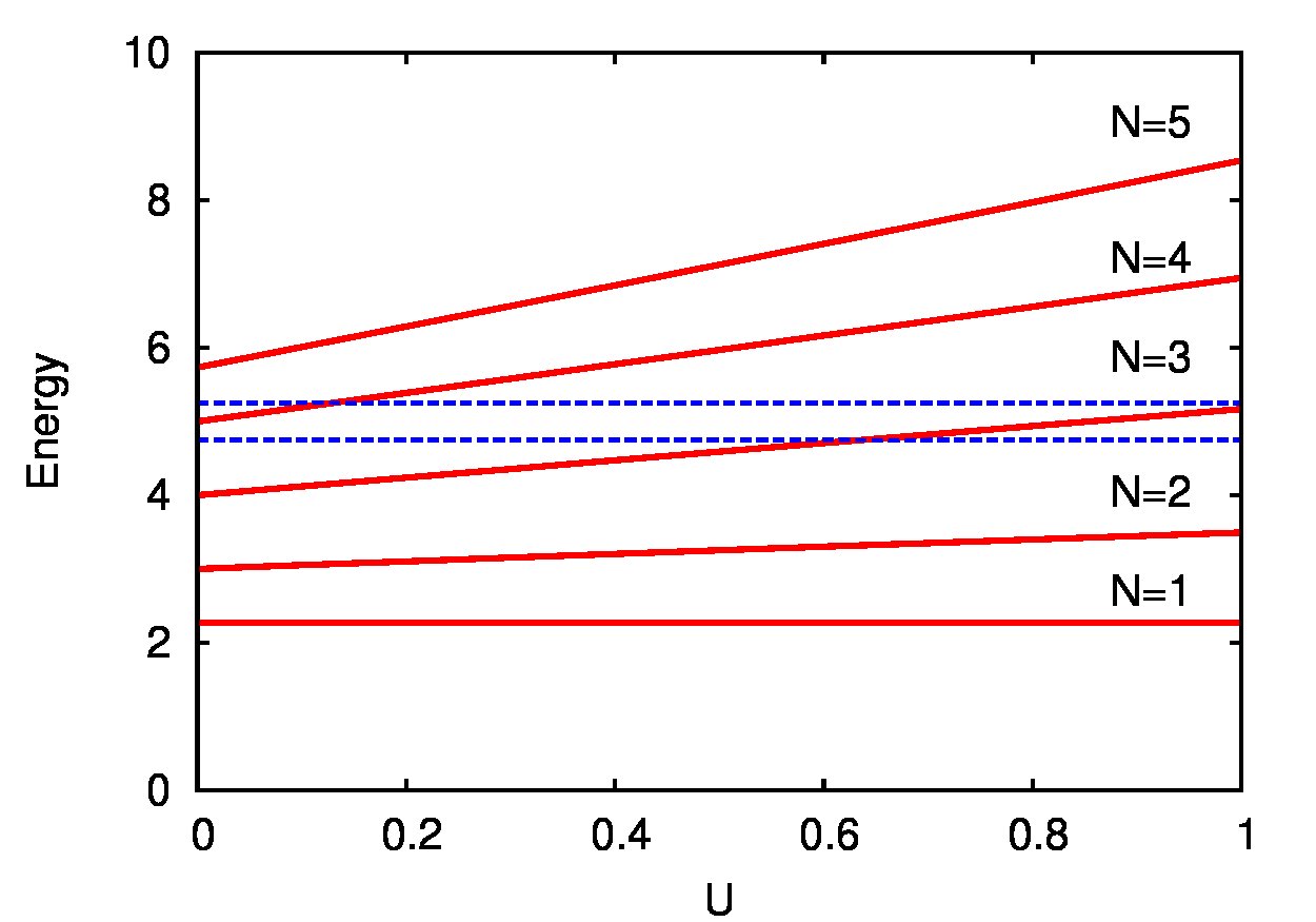
Figure 1: (Color online) The equilibrium chemical potentials $\mu^{(0)}_{N}$ for $1\leq N\leq 5$ as a function of the interaction strength $U$. The dotted lines mark the chemical potentials of the leads selected in the transport simulations shown in the next figure, i. e. $\mu_{L}=5.25$ and $\mu_{R}=4.75$.

The reason to call this a toy model is that we can obtain the complete set of $2^{5}=32$ MES, i. e. we do not need to cut the basis of the 5 SES. We also do not need to cut the MES basis, all matrix elements of the statistical operator can be numerically calculated, even if not all of them might be important for the currents. In addition we will consider the strength of the Coulomb interaction as a free parameter $U$, whereas in a realistic systems this is fixed by the electron charge and the dielectric constant of the material. Our goal is to have a qualitative understanding of the underlying physics, and in particular to show the presence of the Coulomb blocking effects at certain values of $U$ or of the chemical potentials of the leads. The Coulomb matrix elements defined in Eq. (4) are calculated as

$$V_{nm,n^{\prime}m^{\prime}}=\sum_{i\neq i^{\prime}}\phi_{n}^{*}(i)\phi_{m}^{*}(i^{\prime})\,\frac{U}{\mid i-i^{\prime}\mid}\,\phi_{n^{\prime}}(i)\phi_{m^{\prime}}(i^{\prime})\,.$$ (15)

In Fig.1 we show the equilibrium chemical potentials $\mu^{(0)}_{N}$ corresponding to ground states with $1\leq N\leq 5$ particles against the interaction strength $U$. One observes a linear dependence of $\mu^{(0)}_{N}$ on $U$, with slope increasing with $N$. Obviously the total Coulomb energy increases both with $U$ and $N$.

Let us now briefly review the Coulomb blockade scenario. Kouwenhowen Suppose the isolated sample contains $N$ electrons and the chemical potentials of the leads are chosen such that $\mu^{(0)}_{N}<\mu_{R}<\mu_{L}<\mu^{(0)}_{N+1}$. Then the bias window $[\mu_{R},\mu_{L}]$ may include one or more of the excited configurations with $N$ particles. In general some states with $N$ electrons may have excitation energies exceeding $\mu_{L}$ or even $\mu^{(0)}_{N+1}$. This situation corresponds to the Coulomb blockade phenomenon. Indeed, the addition of the $(N+1)$-th electron is energetically forbidden. Consequently the current in the steady state should vanish. However, shorter or longer transient currents are generated by all many-body configurations in the vicinity of the bias window.

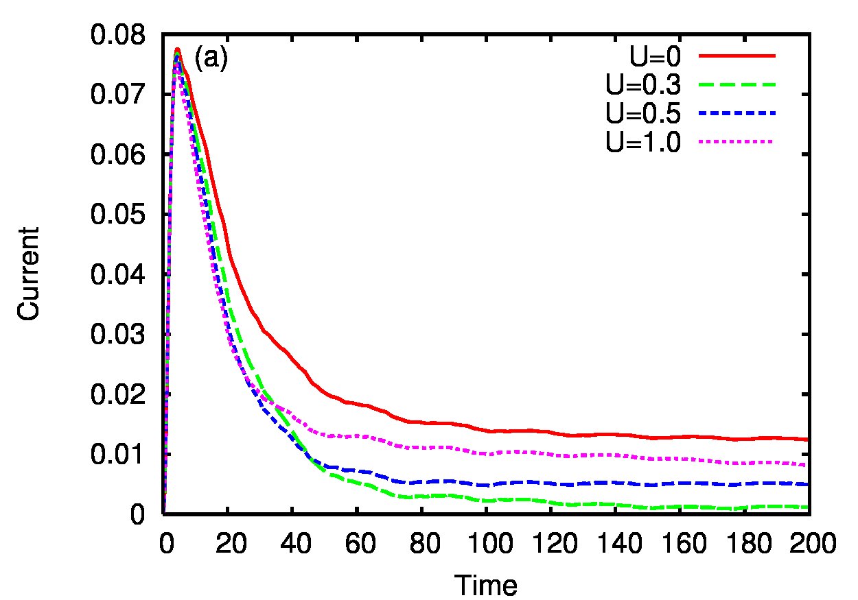
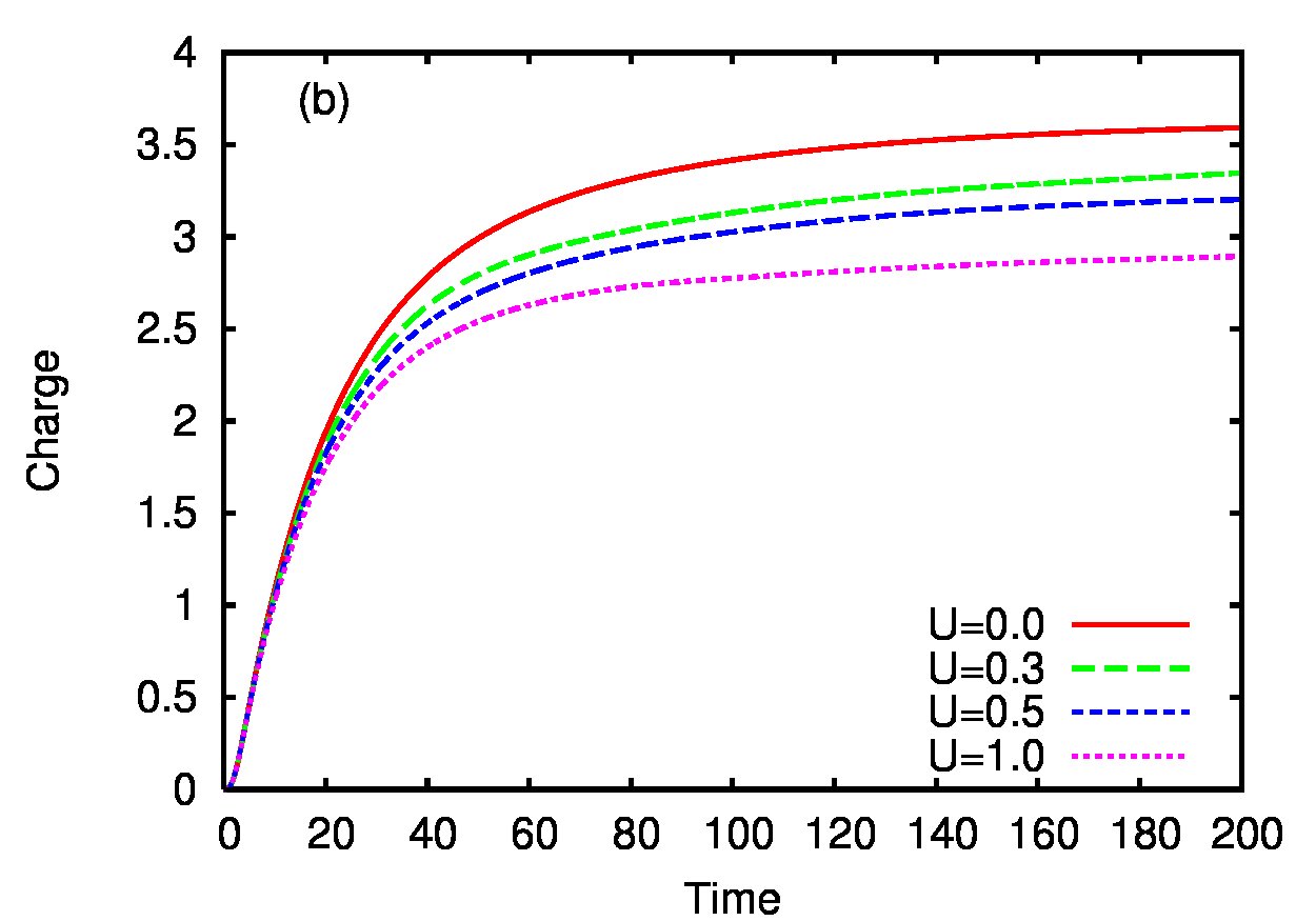
Figure 2: (Color online) The total current entering the $5\times 1$ sample from the left lead as a function of time for the different values of the interaction strength $U$. The chemical potentials of the leads $\mu_{L}=5.25$ and $\mu_{R}=4.75$.

Fig. 2(a) and 2(b) show the total currents in the left lead and the total charge residing in the sample for several values of the interaction strength. $U$ is measured in units of $t_{S}$, the hopping parameter in the sample, NJP1 and the time is expressed in units of $\hbar/t_{S}$ while the current is in units of $et_{S}/\hbar$. The coupling constant in Eq. (13) is $\gamma=1$. The system is initially empty and thus $\rho(0)=|00000\rangle\langle 00000|$.

The chemical potentials of the leads, $\mu_{L}=5.25$ and $\mu_{R}=4.75$, are chosen such that in the absence of Coulomb interaction, i. e. for $U=0$, $\mu^{(0)}_{4}$ is located within the bias window. In this case we obtain in the steady state the mean number of electrons about 3.6 and a non-vanishing current in the leads. This is understandable, since $\mu^{(0)}_{4}=E_{4}=5$, which is the 4-th level of the isolated sample. The occupation of this level in the steady state is about 0.6, the other states being either full or empty. Also in this case, the excited states have small contributions to the steady state current as the system tends to be in the ground state with $N=3$ electrons. Those contributions may also depend on the coupling strength of individual states with the leads, but in general remain small.Valim2

The situation may change for $U\neq 0$. For the interacting system, e. g. for $U=0.3$, the system settles down in the Coulomb blockade regime, the total current being almost suppressed in the steady state. This happens because the interaction pushes the chemical potentials upwards such that for $U=0.3$ both ground states with $N=3$ and $N=4$ electrons are outside the bias window and cannot produce steady currents. When the interaction strength is further increased to $U=0.5$ and $U=1$ the steady state currents are gradually restored. This could look surprising, but one can see in Fig.1 that by increasing $U$ the ground state configuration with 3 electrons approaches and enters the bias window. Consequently the transport becomes again possible. Note that while the steady state currents are not monotonous w.r.t. $U$ the charge absorbed in the system continuously decreases, Fig. 2(b).

Figure 3: The time-dependent total currents in the left and right leads at different values of the chemical potential $\mu_{R}$. The current in the right lead starts at negative values. Other parameters: $V_{L}=V_{R}=0.750$, $U=1.0$.

In transport experiments the strength of the electron-electron interaction is indeed fixed. The usual way to obtain the Coulomb blockade is to vary the chemical potentials of the leads relatively to the energy levels of the sample, or vice versa. In Fig. 3 we show the currents in both leads for different values of the chemical potential $\mu_{R}$, while keeping fixed $\mu_{L}=7$. The strength of the Coulomb interaction is $U=1$ and $\mu^{(0)}_{4}$ almost equals $\mu_{L}$. The steady state value of the current decreases as $\mu_{R}$ increases, because fewer states are included in the bias window. The Coulomb blockade onset occurs for $\mu_{R}>5$, when $\mu^{(0)}_{3}$ drops below $\mu_{R}$. We observe that the maximum value of the total current in the left lead does not change much when $\mu_{R}$ varies. In contrast, the transient current in the right lead is negative and increases in magnitude as $\mu_{R}$ increases. This means that the right lead feeds the many-body configurations that fall below $\mu_{R}$.

The contribution of the excited states to the transient and steady state currents depends strongly on the bias window. In Fig. 4 we show the currents entering the sample from the left lead, carried by the states with $N=2$ and $N=3$ electrons, for $\mu_{R}=3,4,5$ (the cases with non-vanishing current in the steady state). We also show separately the contribution to the currents associated to the ground state configurations, related to $\mu^{(0)}_{2}$ and $\mu^{(0)}_{3}$, and the complementary contribution of all the excited states with 2 and 3 particles. In this case the wave vectors of the ground states are mostly given by the non-interacting wave vectors: $|11000\rangle$ with weight 97% and $|11100\rangle$ with 98% for $N=2$ and $N=3$ respectively.

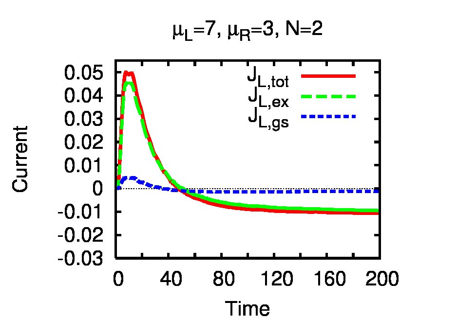
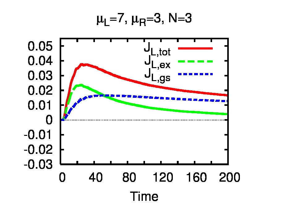
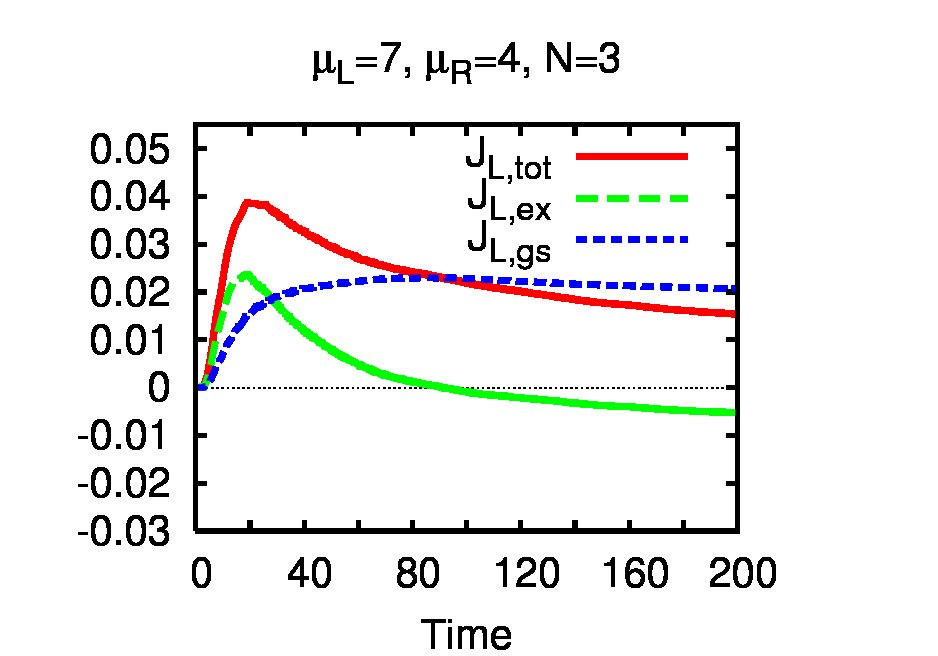
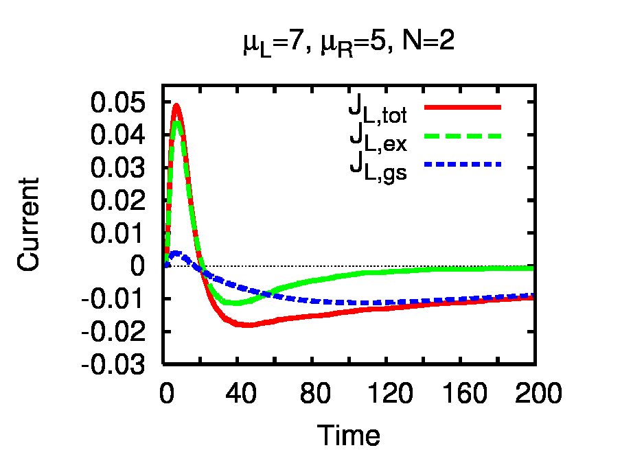
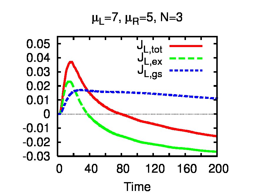
Figure 4: The separate contributions to the current of the ground state with $N$ particles and of all excited states with $N$ particles, for different values of $\mu_{R}$. For completeness we also include the total currents $J_{L}$ for the same configurations. The discussion is made in the text. Other parameters: $V_{L}=V_{R}=0.750$, $U=1.0$.

For $\mu_{R}=3$ the steady state current of the ground state configuration is vanishingly small and so the total negative current associated to two-particle states comes mostly from the excited states. In the many-body energy spectrum of the isolated sample we obtain 5 excited configurations with $\mu^{(i)}_{2}\in[\mu_{R},\mu_{L}]=[3,7]$. As $\mu_{R}$ moves up the steady state current of the ground state with $N=2$ becomes also negative. The combined contributions of the excited states vanishes at $\mu_{R}=5$. As can be seen from Fig. 1 $\mu_{R}=5$ is well above $\mu^{(0)}_{2}$, but very close to $\mu^{(0)}_{3}$. Consequently, the ground configuration with $N=2$ is heavily populated in the steady state, whereas the excited states have low probability and thus weak current. Actually, as we have checked, all the currents associated to each excited state with $N=2$ vanish individually. In the transient regime however the $N=2$ currents in all three cases are dominated by the excites states.

The currents of the excited states having $N=3$ electrons are positive at $\mu_{R}=3$, but change sign at $\mu_{R}=4$. For $\mu_{R}=5$ their magnitude exceeds the contribution of the ground state which is always positive. A more detailed analysis of the currents carried by specific excited states will be given for the 2D model.

Finally, both in the transient and in the steady states the currents have small periodic fluctuations determined by the permanent transitions of electrons between the states in the sample and the states in the leads and back.Valim2 They are best seen in Fig. 2(a). Such fluctuations have also been obtained very recently by Kurth et al. using combination of the non-equilibrium Green’s functions and the time dependent density-functional theory of the Coulomb interaction.Kurth2

III.2 2D lattice

We show now results for a 2D rectangular lattice with $12\times 10$ sites. For a lattice constant of $a=5$ nm this sample can be seen as a discrete version of a quantum dot of 60 nm $\times$ 50 nm. We used the lowest 10 SES of the non-interacting sample in the numerical diagonalization of the interacting Hamiltonian. This number is sufficient to produce convergent results for the first 50 MES for an interaction strength $U=0.8$. The Coulomb matrix elements are calculated in the same way as for the 1D case, Eq. (15), except that now the site indices are two-dimensional, i. e. $i=(i_{x},i_{y})$ and $i^{\prime}=(i^{\prime}_{x},i^{\prime}_{y})$.

The two contact sites are chosen at diagonally opposite corners of the sample. The coupling coefficients are calculated with Eq. (14), like for the 1D chain, and depend on the wave function of the particular SES at the contact sites. These coefficients are illustrated in Fig. 5(a). The reduced density matrix is calculated using the first 50 MES. This allowed us to take into account many-body configurations with up to 3 electrons.

In Fig. 5(b) we show the chemical potentials $\mu^{(i)}_{N}$ for the ground and excited states with $N=1,2,\ \mathrm{and}\ 3$ particles. At the initial moment $t_{0}=0$ the system is empty. Based on the previous example, the main contribution to the currents in the steady states is expected from those MES with ground state chemical potentials located inside the bias window $[\mu_{R},\mu_{L}]$. One also observes excited configurations with $N$ particles having chemical potentials larger than $\mu^{(0)}_{N+1}$.

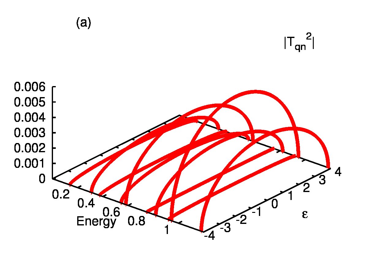
Figure 5: (Color online) (a) The coupling amplitudes $|T_{qn}|^{2}$ for $n=1,..,5$ between single-particle states in the leads with momentum $q$ and the lowest 5 single-particle states of the isolated dot. (b) The generalized chemical potentials for $N$ -particle interacting configurations. The red crosses mark $\mu^{(0)}_{N}$ while the other ones correspond to generalized potentials $\mu^{(i)}_{N}$ related to the $i$-th excited state of the $N$ particle system.

In the following we discuss the currents carried by the various many-body states involved in transport. In a first series of calculations we selected the chemical potential $\mu_{R}=0.2$ and used two values of the chemical potential of the left lead $\mu_{L}=0.4$ and $\mu_{L}=0.6$. For $\mu_{R}=0.2$ and $\mu_{L}=0.4$ the bias window contains only the 1-st and the 2-nd excited configurations with $N=1$, Fig. 5(b). The ground states for $N=1$ and $N=2$ are instead located below and above the bias window, respectively. Consequently the steady state current is very small. When $\mu_{L}$ increases to 0.6 the ground state configuration with $N=2$ enters the bias window and the current increases, Fig. 6(a).

To analyze the transient regime we split the current into contributions given by the ground state and excited states with 1 electron (see Fig. 6(b)). When $\mu_{L}=0.4$ the 1-st and 2-nd excited state carry currents exceeding the current associated to the ground state, which survive all the way to the steady state. The current corresponding to the 2-nd excited state is smaller than the current of the 1-st excited state, but comparable to that of the ground state. This is explained by the strength of the coupling coefficients shown in Fig. 5(a), the 2-nd single-particle state being stronger coupled to the leads. The remaining higher excited states give oscillating and fast decaying transient currents. In Fig. 6(c) $\mu_{L}=0.6$ and therefore higher excited states enter the bias window; their transient currents are still decaying but at a smaller rate. Comparing with Fig. 6(a) it in clear that the transient regime is dominated by excited states.

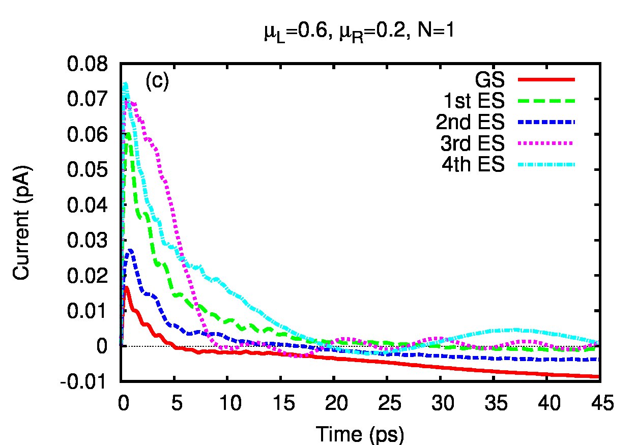
Figure 6: (a) The total currents in the left and right leads for $\mu_{L}=0.6$ and $\mu_{L}=0.4$, while keeping $\mu_{R}=0.2$. (b) The partial currents in the left lead for single-particle states when $\mu_{L}=0.4$ and $\mu_{R}=0.2$. (c) The partial currents in the left lead for single-particle states when $\mu_{L}=0.6$ and $\mu_{R}=0.2$

Figure 7: (a) The total current in the left lead carried by all many-body configurations with $N=2$, for increasing values of $\mu_{L}$ (i. e. 0.6,0.7,0.8 and 0.9) and $\mu_{R}=0.2$. (b) The same for $N=3$.

Next we discuss currents associated with states having 2 and 3 electrons. We keep now fixed $\mu_{R}=0.35$ and again increase $\mu_{L}$ starting with 0.6. Fig. 7(a) shows the total currents in the left lead for $N=2$ and $N=3$. As the bias increases the transient currents are enhanced, but they become comparable as the system approaches the steady state. In Fig. 7(b) the total current on three particle states shows a different behavior: the steady states value increases drastically when $\mu_{L}$ moves up. To explain this one can look again at the diagram of the chemical potentials, Fig. 5(b). At $\mu_{L}=0.6$ the 3-particle configurations are above the bias window and as such they contribute less to the current. In contrast, as $\mu_{L}$ increases the ground state configuration with $N=3$ enters the bias window, the window is closer to the excited states, and thus the total current increases. Actually, for $\mu_{L}=0.8$ and $0.9$ the current for $N=3$ does not reach the steady state in the time interval considered.

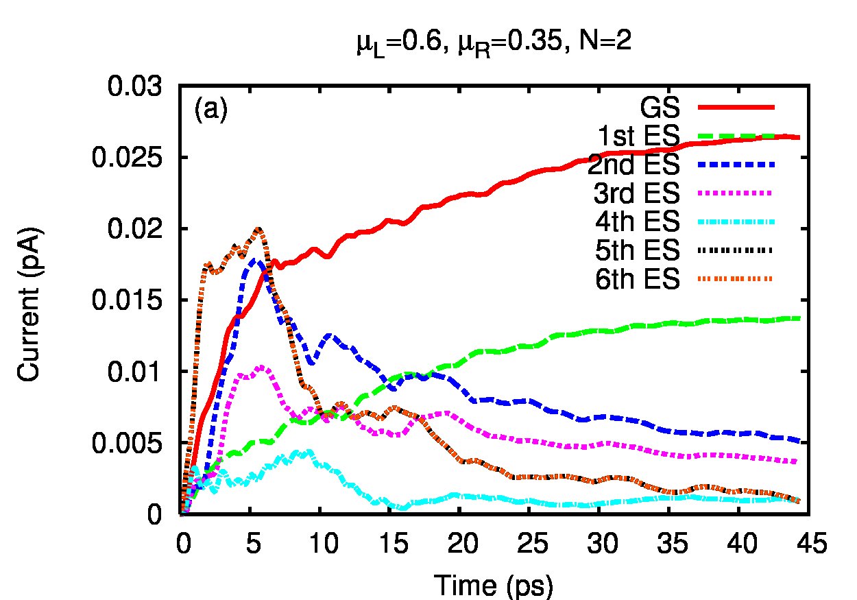
Figure 8: (a) The total current in the left lead carried by all many-body configurations with $N=2$ at $\mu_{L}=0.6$. (b) The same for $\mu_{L}=0.9$. Other parameters $\mu_{R}=0.35$.

Now we look at the contribution of the excited states with $N=2$ for two cases, $\mu_{L}=0.6$ and $\mu_{L}=0.9$. Again, the inspection of the diagram in Fig. 5(b) predicts the results of Fig. 8. When $\mu_{L}=0.6$ there is just one excited configuration within the bias window, in addition to the ground state. In Fig. 8(a) we see that in the steady state these two configurations give significant contributions to the current, whereas the higher excited states play a role only in the transient regime. Fig. 8(b) shows that at $\mu_{L}=0.9$ the currents of the excited states and of the ground state are decreasing, some of them reaching even negative values towards the steady state. This happens because the bias window includes now the ground state with $N=3$ and the excited states with $N=2$ deplete in the favor of the ground state.

The sign of the current carried by states with $N$ particles depends on the placement of the corresponding ground state chemical potential relatively to the bias window. For example if we fix $\mu_{L}=1.5$ and $\mu_{R}=0.65$ we obtain $\mu_{2}^{(0)}<\mu_{L}$. Fig. 9(a) shows the $N$-particle currents when the sample initially contains two electrons in the ground state. This initial state evolves faster to the steady state than the empty system. While for $N=3$ the current in the left lead is positive, for both $N=2$ and $N=1$ the currents are negative. The charge residing on each $N$-particle state and the total charge are shown in Fig. 9(b). Since single-particle configurations are unlikely their occupation vanishes. The total charge accumulated on the $N=3$ states increases up to 2, while the total charge on the $N=2$ states decreases from 2 to 0.75. The sign of the current for $N=2$ becomes positive when $\mu_{R}$ is lowered to 0.2, Fig. 9(c), and exceeds the current carried by the states with $N=3$. This is because the 1-st and the 2-nd SES practically determine the ground state with two electrons and thus $\mu_{2}^{(0)}$, and also because the 1-st SES is strongly coupled to the leads. However, the current with $N=1$ is still negative.

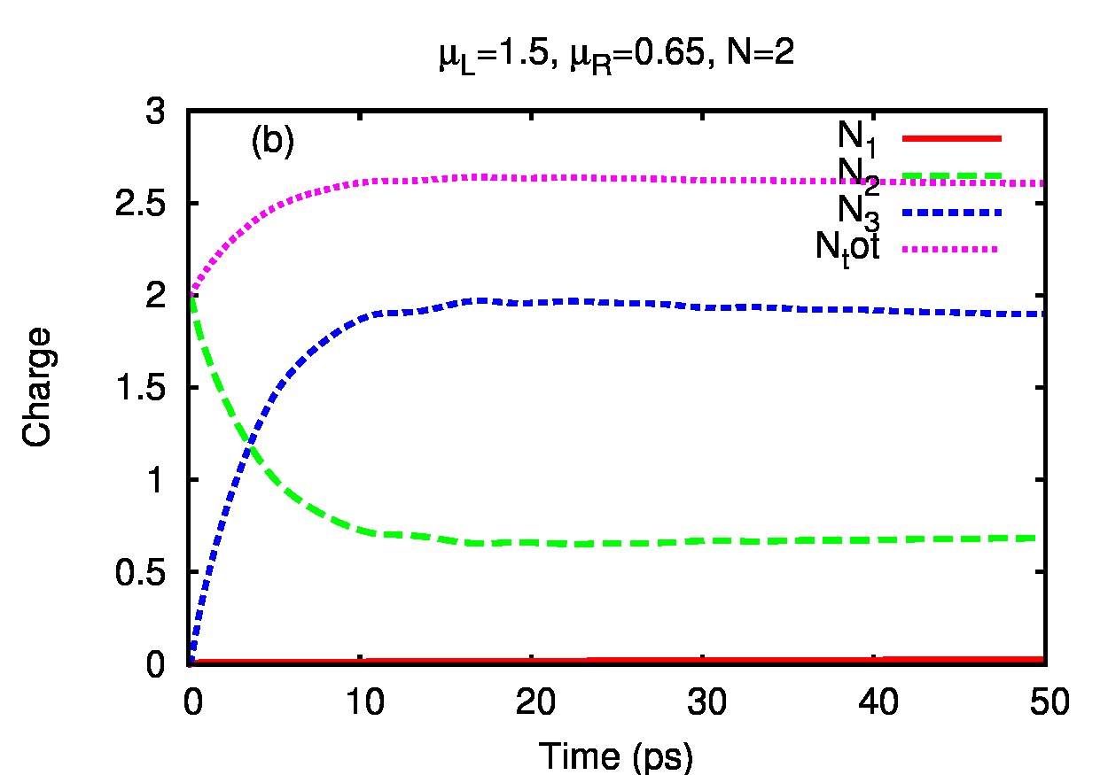
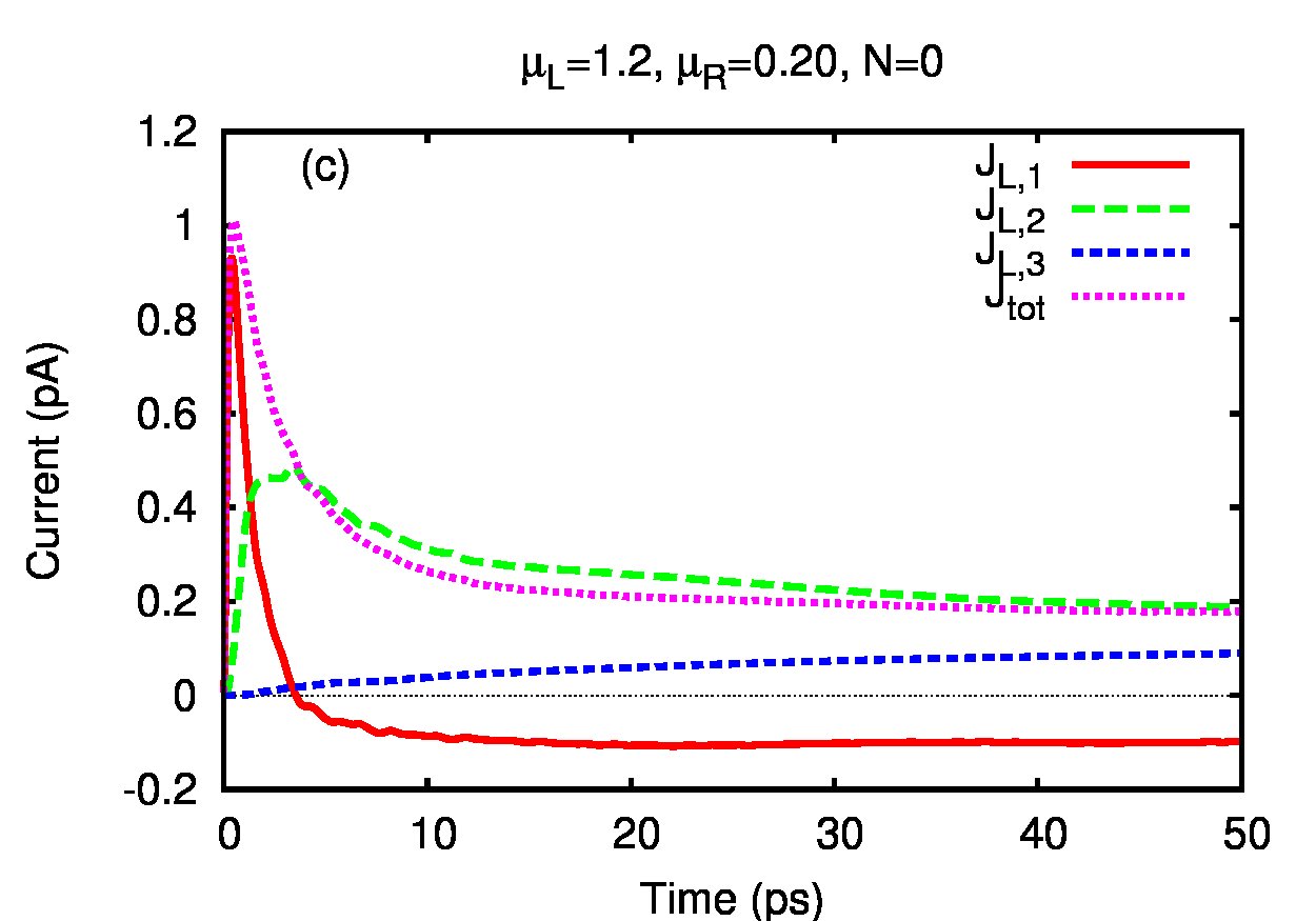
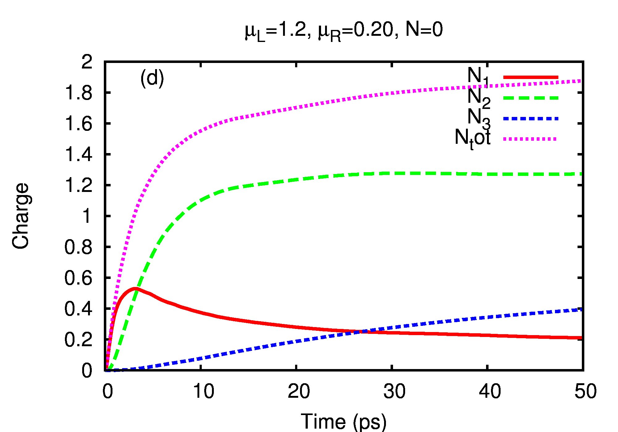
Figure 9: (a) The total current in the left lead carried by $N$-particle states and the total charge. for $\mu_{L}=1.5$ and for $\mu_{R}=0.65$. (b) The occupation number of the $N$-particle states. (c) The total current in the left lead carried by $N$-particle states for $\mu_{L}=1.2$ and $\mu_{R}=0.2$. (d) The occupation number of the $N$-particle states and the total charge.

III.3 Parabolic quantum wire

In this subsection we apply the GME with Coulomb interaction to describe the transport through a short quantum wire of length $L_{x}=300$ nm with a parabolic confinement in the $y$-direction perpendicular to the direction of transport. The contact ends of the isolated wire at $\pm L_{x}/2$ are described by hard walls. This is now a continuous model, where a large functional basis is used to expand the eigenfunctions of the system in. In a similar manner we use a functional basis with complete truncated sets of continuous and discrete functions to expand the eigenfunctions of the semi-infinite parabolic leads in. To show that we can describe the combined geometrical effects imposed on the system by it’s geometry and an external perpendicular magnetic field we place the quantum wire is in an external magnetic field of strength $1.0$ T. The characteristic confinement energy is given by $\hbar\Omega_{0}=1.0$ meV. We assume GaAs parameters with $m^{*}=0.067m_{e}$, $\kappa=12.4$ meV. The magnetic length modified by the parabolic confinement is $a_{w}=\sqrt{\hbar/(m^{*}\Omega_{w})}$, with $\Omega_{w}^{2}=\Omega_{0}^{2}+\omega_{c}^{2}$. and the cyclotron frequency $\omega_{c}=eB/(m^{*}c)$. At $B=1.0$ T, $a_{w}=23.87$ nm. The semi-infinite leads having the same parabolic confinement and being subject to the same external perpendicular magnetic field have a continuous energy spectrum with discrete Landau sub-bands.

The Coulomb potential in Eq. (4) in the 2D wire is described by

$$u(\mathbf{r}-\mathbf{r}^{\prime})=\frac{e^{2}}{\kappa\sqrt{(x-x^{\prime})^{2}+(y-y^{\prime})^{2}+\eta^{2}}},$$ (16)

with the small convergence parameter $(\eta/a_{w})=0.01$ to facilitate the two-dimensional numerical integration needed for the matrix elements (4).

After the GME (9) has been transformed to the interacting many-electron basis by the unitary transformation obtained by the diagonalization of $H_{S}$ (3) we truncate the RDO (8) to 32 MES. For the bias range $0.0\leq\Delta\mu=\mu_{L}-\mu_{R}\leq 1.7$ meV used here 10 SES are sufficient to obtain these lowest 32 states with good accuracy. We will be omitting singly occupied states of high energy that should not be relavant for the parameters here. The natural strength of the Coulomb interaction will only give us MES that are occupied by one or two electrons in the energy range 0 to 6 meV covered by the 32 MES.

Since in the partitioning approach $[H_{S},H_{L}]=0$ we have to construct $T^{l}_{qn}$ as a non-local overlap of $\phi_{n}$ and $\psi_{q}^{L,R}$ on the contact regions ${\cal C}_{l},\,l=L,R$: NJP2

$$T^{l}_{qn}=\int_{{\cal C}_{l}}d{\bf r}d{\bf r^{\prime}}\left(\psi^{*}_{ql}({\bf r})\phi_{n}({\bf r})g^{l}_{qn}({\bf r},{\bf r^{\prime}})+h.c.\right).$$ (17)

$$g^{l}_{qn}({\bf r},{\bf r^{\prime}})=g_{0}^{l} \exp{\left[-\delta_{1}^{l}(x-x^{\prime})^{2}-\delta_{2}^{l}(y-y^{\prime})^{2}\right]}$$

$$\times \exp{\left(\frac{-|E_{n}-\varepsilon_{ql}|}{\Delta_{E}^{l}}\right)}\,.$$ (18)

As before $\varepsilon_{ql}$ is the energy spectrum of lead $l$, and $E_{n}$ is the energy of the SES numbered by $n$ in the quantum wire. The quantum number $q$ for the states in leads represents both the discrete Landau band number and a continuous quantum number that can be related to the momentum of a particular state. Here we use the parameters $\delta_{1}a_{w}^{2}=\delta_{2}a_{w}^{2}=0.25$, $\Delta_{E}^{LR}=0.25$ meV, and $g_{0}^{LR}=40$ meV for $B=1.0$ T. The domain of the overlap integral for the leads is $\pm 2a_{w}$ into the lead or the system for $x$ and $x^{\prime}$ from each end of the wire at $\pm L_{x}/2$ and between $\pm 4a_{w}$ for $y$ and $y^{\prime}$, see Ref. (NJP2, ) for an exact definition. All the SES will be coupled to the leads, but the coupling strength will depend on the character of the SES, whether it is an edge- or bulk state and other finer geometrical details that is brought about by the magnetic field.

The right chemical potential $\mu_{R}$ is held at $1.4$ meV and the transport properties are calculated for different values of the bias $\Delta\mu$ by varying $\mu_{L}$. Figure 10 compares the total occupation of all one- electron and two-electron MES for the interacting system at two different values of the bias.

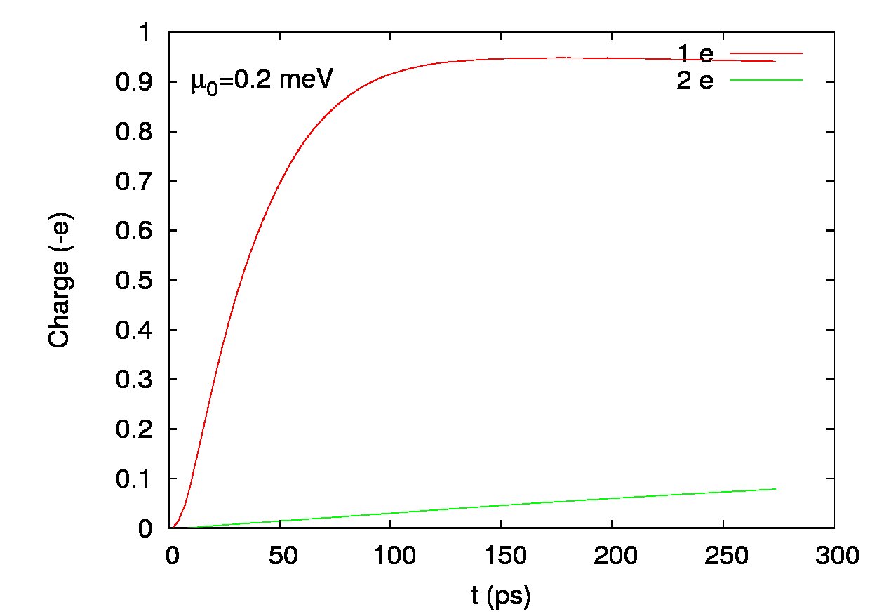
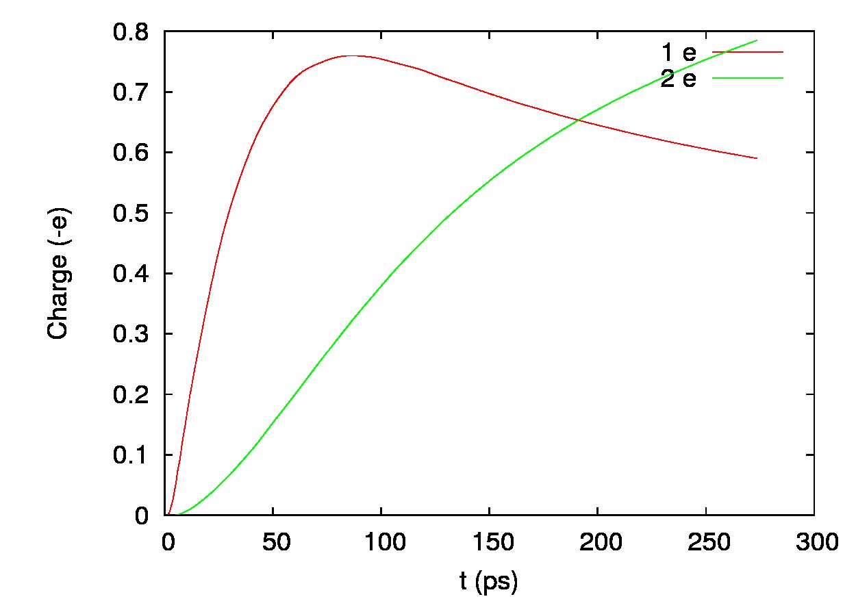
Figure 10: (Color online) The total charge residing in one- and two-electron states as a function of time for two different values of the bias $\Delta\mu$. $B=1.0$ T, $L_{x}=300$ nm, $\hbar\Omega_{0}=1.0$ meV.

At, $\Delta\mu=0.2$ meV we see that almost solely one-electron states are occupied, while for $\Delta\mu=1.2$ meV initially it is likely to have one-electron states occupied, but very soon the occupation of the two-electron states becomes as probable with the likelihood of the occupation of the one-electron states fast reducing with time. We also have to admit here that even though the steady state value of the total current through the system can be deduced by the values of the current at 270 ps, the charging of the system takes much longer time, since we are using here a very weak coupling to the leads that mimics a tunneling regime.

If we now use the average value of the current in the left and right leads at $t=270$ ps as a measure of the steady state current we get the information displayed in Fig. 11,

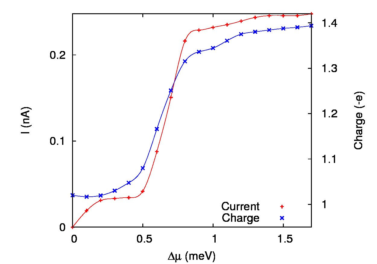
Figure 11: The total steady state current for interacting 10 SES, and the total charge at $t=270$ ps. for different values of the bias $\Delta\mu$. $B=1.0$ T, $L_{x}=300$ nm, $\hbar\Omega_{0}=1.0$ meV.

where the steady state value of the current is shown for the interacting system as a function of the bias and compared to the charge in the system. We have a clear Coulomb blocking in the interacting system. In the case of a non-interacting system the lack of a gap between the one- and two electron MES and a strong mixing of the energy regimes of two- and three-electron states the two-electron plateau only appears as a small shoulder. The 32 MES selected here include no three-electron or MES with higher number of electrons. It should be mentioned here that a different choice of the right bias $\mu_{R}$ can result in the system charging faster and thus at the same time the total current through it being smaller. This comes from the fact that the states have a different coupling to the leads and the time range shown here is very much in the transient- or it’s long exponential decay regime.

Figure 12 displaying the current in the right lead gives an idea how the Coulomb blocking plateau appears after the transition regime.

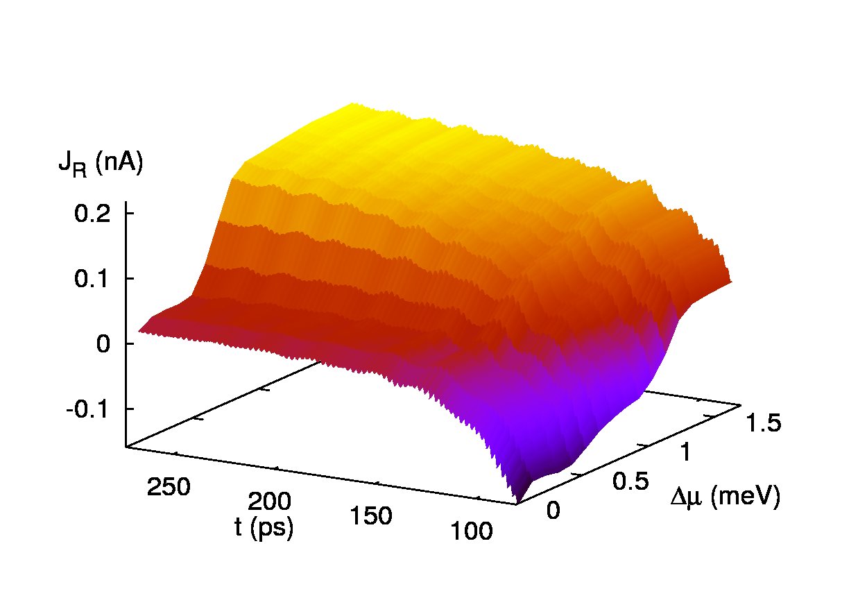
Figure 12: The total current in the right lead for interacting and non-interacting 10 SES as a function of the bias $\Delta\mu$ and time. $B=1.0$ T, $L_{x}=300$ nm, $\hbar\Omega_{0}=1.0$ meV.

The transition regime where the right current goes negative, i. e. where it supplies charge to the system is partially truncated from the figure.

IV Summary and conclusions

We calculated time-dependent currents in open mesoscopic systems composed by a sample attached to two semi-infinite leads, by solving the generalized master equation for the reduced density operator acting in the Fock space of the sample. This is the natural framework for including the Coulomb electron-electron interaction in the sample, which is the main achievement of this work. The Coulomb interaction is treated in the spirit of the exact diagonalization method, i. e. in a pure many-body manner. The interacting many-body states of the sample are expanded in the basis of non-interacting “bit-string” states with unspecified number of electrons. We believe our method is a viable alternative to a recent approach based on a time-dependent density-functional model.Kurth ; Myohanen ; Kurth2 We used three sample models, a short 1D wire with 5 sites, but also a larger 2D lattice with 120 sites and a continuous model, whereas the cited group used much smaller samples even with no structure.Kurth2

Indeed, due to computational limitations we could use only a restricted, effective number of many-body states in the GME, between 30-50 depending on the model, from the bottom of the energy spectrum. We chose the bias window $[\mu_{R},\mu_{L}]$ and the strength of the sample-leads coupling parameters $V_{R,L}$ such that only the effective states contribute to the transport of electrons through the sample, whereas the states with higher energy are unreachable by the electrons. Consequently the number of electrons in the sample can be only up to 3 or 4.

We could calculate the contribution to the charge and currents in the sample and in the leads respectively, corresponding to any particular many-body state. We use the 1D chain as a toy model to emphasize the dominant role of the excited states in the transient regime and the onset of the Coulomb blockade in the steady state. A similar 1D model with 4 sites 1D has been considered recently by Myöhänen et al.Myohanen

As shown also in our previous works on time-dependent transport in non-interacting systems the GME method includes information on the energy structure of the sample, but also on the geometrical properties reflected in the wave functions and sample-lead contacts.NJP1 ; NJP2 ; Valim2 Here we illustrate these aspects, in the interacting case, for two nanosystems: a two-dimensional quantum dot described by a lattice Hamiltonian and a short parabolic quantum wire. The time-dependent occupation of specific many-body states was thoroughly analyzed, for different values of the chemical potentials of the leads. It turned out that the excited states with $N$ electrons contribute to the steady state currents if the ground state configuration with $N+1$ particles is not available for transport. However, if $\mu^{(0)}_{N}<\mu_{R}$ and at the same time $\mu^{(0)}_{N+1}$ lies within the bias window the excited states with $N$ particles are active only in the transient regime and become de-populated in the steady state regime. This behavior is of interest in the excited-state spectroscopy experiments.Tarucha To our knowledge the time-dependent currents associated to excited states have not been discussed theoretically so far.

- (1) G. Stefanucci, S. Kurth, A. Rubio and E. K. U. Gross, Phys. Rev. B 77, 075339 (2008).
- (2) V. Moldoveanu, A. Manolescu and V. Gudmundsson, Phys. Rev. B 76, 085330 (2007)
- (3) X. Zheng, F. Wang, C. Y. Yam, Y. Mo, and G.H. Chen, Phys. Rev. B 75, 195127 (2007).
- (4) V. Gudmundsson, G. Thorgilsson, C-S Tang, and V. Moldoveanu, Phys. Rev. B 77, 035329 (2008).
- (5) U. Harbola, M. Esposito, and S. Mukamel, Phys. Rev. B 74, 235309 (2006).
- (6) S. Welack, M. Schreiber, and U. Kleinekathöfer, J. Chem. Phys. 124, 044712 (2006)
- (7) V. Moldoveanu, A. Manolescu and V. Gudmundsson, New J. Phys. 11, 073019 (2009).
- (8) V. Gudmundsson, C. Gainar, C-S Tang, V. Moldoveanu, A. Manolescu, to appear in New J. Phys.
- (9) S. Kurth, G. Stefanucci, C.-O. Almbladh, A. Rubio, and E. K. U. Gross, Phys. Rev. B 72, 035308 (2005).
- (10) P. Myöhänen, A. Stan, G. Stefanucci, and R. van Leeuwen, Phys. Rev. B 80, 115107 (2009), Europhys. Lett. 84, 67001 (2008).
- (11) T. Fujisawa, D. G. Austing, Y. Tokura, Y. Hirayama, and S. Tarucha, J. Phys.: Condens. Matter 15, R1395 (2003).
- (12) D. C. Langreth and P. Nordlander, Phys. Rev. B 43, 2541 (1991)
- (13) S. A. Gurvitz and Ya. S. Prager, Phys. Rev. B 53, 15932 (1996).
- (14) J. König, H. Schoeller, and G. Schön, Phys. Rev. Lett. 76, 1715 (1996); J. König, J. Schmid, H. Schoeller, and G. Schön, Phys. Rev. B 54, 16 820 (1996).
- (15) D. Becker and D. Pfannkuche, Physical Review B 77 205307 (2008).
- (16) S. Nakajima, Prog. Theor. Phys. 20, 948 (1958).
- (17) R. Zwanzig, J. Chem. Phys. 33, 1338 (1960).
- (18) C. Timm, Phys. Rev. B 77, 195416 (2008).
- (19) X. Q. Li and Y. J. Yan, Phys. Rev. B 75, 075114 (2007).
- (20) M.Esposito and M. Galperin, Phys. Rev. B 79, 205303 (2009).
- (21) D. Darau, G. Begemann, A. Donarini, and M. Grifoni, Physical Review B 79 235404 (2009).
- (22) C. Caroli, R. Combescot, P. Nozieres, and D. Saint-James, J. Phys. C 4, 916 (1971).
- (23) E. Vaz, J. Kyriakidis, J. Chem. Phys. 129, 024703 (2008)
- (24) L.P. Kouwenhouven et al., in Mesoscopic Electron Transport, edited by L.L. Sohn, L.P. Kouwenhouven, and G. Schön, NATO Advanced Study Institute, Series E, Vol. 345 (Kluwer, Dordrecht, 1997).
- (25) V. Moldoveanu, A. Manolescu and V. Gudmundsson, Phys. Rev. B 80, 205325 (2009).
- (26) S. Kurth, G. Stefanucci, E. Khosravi, C. Verdozzi, ad E. K. U. Gross, e-print arXiv:0911.3870 [cond-mat.mes-hall] (2009).