$b\to s\ell^{+}\ell^{-}$ in the high $q^{2}$ region at two-loops

Abstract:

We report on the first analytic NNLL calculation for the matrix elements of the operators $O_{1}$ and $O_{2}$ for the inlusive process $b\to X_{s}l^{+}l^{-}$ in the kinematical region $q^{2}>4m_{c}^{2}$, where $q^{2}$ is the invariant mass squared of the lepton-pair.

1 Introduction

In the Standard Model, the flavor-changing neutral current process $b\to X_{s}l^{+}l^{-}$ only occurs at the one-loop level and is therefore sensitive to new physics. In the kinematical region where the lepton invariant mass squared $q^{2}$ is far away from the $c\bar{c}$-resonances, the dilepton invariant mass spectrum and the forward-backward asymmetry can be precisely predicted using large $m_{b}$ expansion, where the leading term is given by the partonic matrix element of the effective Hamiltonian

$$\mathcal{H}_{eff}=-\frac{4G_{F}}{\sqrt{2}}V_{ts}^{*}V_{tb}\sum\limits_{i=1}^{10}C_{i}(\mu)O_{i}(\mu).$$ (1)

We neglect the CKM combination $V_{us}^{*}V_{ub}$ and the operator basis is defined as in [1]. In [2] we published the first analytic NNLL calculation of the high $q^{2}$ region of the matrix elements of the operators

$$O_{1}=(\bar{s}_{L}\gamma_{\mu}T^{a}c_{L})(\bar{c}_{L}\gamma^{\mu}T^{a}b_{L}),\qquad O_{2}=(\bar{s}_{L}\gamma_{\mu}c_{L})(\bar{c}_{L}\gamma^{\mu}b_{L})\,,$$ (2)

which dominate the NNLL amplitude numerically. Earlier these results were only available analytically in the region of low $q^{2}$ [3, 4]. Using equations of motion the NNLL matrix elements of the effective operators take the form

$$\langle s\ell^{+}\ell^{-}|O_{i}|b\rangle_{\text{2-loops}}=-\left(\frac{\alpha_{s}}{4\pi}\right)^{2}\left[F_{i}^{(7)}\langle O_{7}\rangle_{\text{tree}}+F_{i}^{(9)}\langle O_{9}\rangle_{\text{tree}}\right],$$ (3)

where $O_{7}=e/g_{s}^{2}m_{b}(\bar{s}_{L}\sigma^{\mu\nu}b_{R})F_{\mu\nu}$ and $O_{9}=e^{2}/g_{s}^{2}(\bar{s}_{L}\gamma_{\mu}b_{L})\sum_{l}(\bar{l}\gamma^{\mu}l)$.

2 Calculations

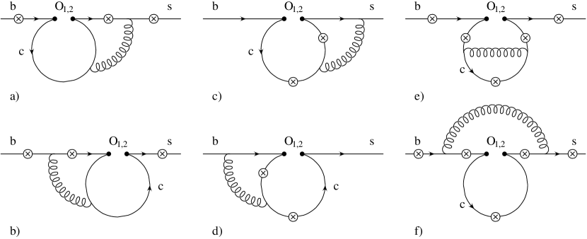
Figure 1: Diagrams that have to be taken into account at order $\alpha_{s}$. The circle-crosses denote the possible locations where the virtual photon is emitted (see text).

The diagrams contributing at order $\alpha_{s}$ are shown in Figure 1. We set $m_{s}=0$ and define

$$\hat{s}=\frac{q^{2}}{m_{b}^{2}}\quad\mbox{and}\quad z=\frac{m_{c}^{2}}{m_{b}^{2}},$$ (4)

where $q$ is the momentum of the virtual photon. After reducing occurring tensor-like Feynman integrals [5] the remaining scalar integrals can be further reduced to master integrals using integration by parts (IBP) identities [6]. Considering the region $\hat{s}>4z$, we expanded the master integrals in $z$ and kept the full analytic dependence in $\hat{s}$.

For power expanding Feynman integrals we use a combination of method of regions [7] and differential equation techniques [8, 9]: Consider a set of Feynman integrals $I_{1},\ldots,I_{n}$ depending on the expansion parameter $z$ and related by a system of differential equations obtained by differentiating $I_{\alpha}$ with respect to $z$ and applying IBP identities:

$$\frac{d}{dz}I_{\alpha}=\sum_{\beta}h_{\alpha\beta}I_{\beta}+g_{\alpha},$$ (5)

where $g_{\alpha}$ contains simpler integrals which pose no serious problems. Expanding both sides of (5) in $\epsilon$, $z$ and $\ln z$

$$I_{\alpha}=\sum_{i,j,k}I_{\alpha,i}^{(j,k)}\epsilon^{i}z^{j}(\ln z)^{k},\qquad h_{\alpha\beta}=\sum_{i,j}h_{\alpha\beta,i}^{(j)}\epsilon^{i}z^{j},\qquad g_{\alpha}=\sum_{i,j,k}g_{\alpha,i}^{(j,k)}\epsilon^{i}z^{j}(\ln z)^{k},$$ (6)

and inserting (6) into (5) we obtain algebraic equations for the coefficients $I_{\alpha,i}^{(j,k)}$

$$0=(j+1)I_{\alpha,i}^{(j+1,k)}+(k+1)I_{\alpha,i}^{(j+1,k+1)}-\sum_{\beta}\sum_{i^{\prime}}\sum_{j^{\prime}}h_{\alpha\beta,i^{\prime}}^{(j^{\prime})}I_{\beta,i-i^{\prime}}^{(j-j^{\prime},k)}-g_{\alpha,i}^{(j,k)}.$$ (7)

This enables us to recursively calculate higher powers of $z$ once the leading powers are known. In practice this means that we need the $I_{\alpha,i}^{(0,0)}$ and sometimes also the $I_{\alpha,i}^{(1,0)}$ as initial condition to (7). These initial conditions can be computed using method of regions. A non trivial check is provided by the fact that the leading terms containing logarithms of $z$ can be calculated by both method of regions and the recurrence relation (7).

The summation index $j$ in (6) can take integer or half-integer values, depending on the specific set of integrals $I_{\alpha}$. In order to determine the possible powers of $z$ and $\ln(z)$ we used the algorithm described in [9]. A given $D$-dimensional $L$-loop Feynman integral $I(z)$ reads in Feynman parameterization

$$I(z)=(-1)^{N}\left(\frac{i}{(4\pi)^{D/2}}\right)^{L}\Gamma(N-LD/2)\int d^{N}x\,\delta(1-\sum_{n=1}^{N}x_{n})\frac{U^{N-(L+1)D/2}}{(zF_{1}+F_{2})^{N-LD/2}},$$ (8)

where $U$, $F_{1}$ and $F_{2}$ are polynomials in $x_{n}$. Using Mellin-Barnes representation (8) can be cast into the following form

$$\begin{split}I(z)=\,&(-1)^{N}\left(\frac{i}{(4\pi)^{D/2}}\right)^{L}\frac{1}{2\pi i}\int_{-i\infty}^{i\infty}ds\,z^{s}\Gamma(-s)\Gamma(s+N-LD/2)\\ \,&\times\int d^{N}x\,\delta(1-\sum_{n=1}^{N}x_{n})U^{N-(L+1)D/2}F_{1}^{s}F_{2}^{-s-N+LD/2}.\end{split}$$ (9)

By closing the integration contour over $s$ to the right hand side the poles on the positive real axis turn into powers of $z$. If we apply the technique of sector decomposition [10] to (9) we end up with terms of the following form

$$\sum_{l=1}^{N}\sum_{k}\int_{0}^{1}d^{N-1}t\left(\prod_{j=1}^{N-1}t_{j}^{A_{j}-B_{j}\epsilon-C_{j}s}\right)U_{lk}^{N-(L+1)D/2}F_{1,lk}^{s}F_{2,lk}^{-s-N+LD/2},$$ (10)

where $U_{lk}$, $F_{1,lk}$ and $F_{2,lk}$ contain terms that are constant in $\vec{t}$. From (10) we can read off that the poles in $s$ are located at:

$$s_{jn}=\frac{1+n+A_{j}-B_{j}\epsilon}{C_{j}},$$ (11)

where $n\in\mathbb{N}_{0}$.

Additionally, the procedure described above allows us to evaluate the coefficients of the expansion in $z$ numerically which we used to again test the initial conditions of the differential equations.

3 Results

Figure 2: Real and imaginary parts of the form factors $F_{1,2}^{(7,9)}$ as functions of $\hat{s}$. To demonstrate the convergence of the expansion in $z$ we included all orders up to $z^{6}$, $z^{8}$ and $z^{10}$ in the dotted, dashed and solid lines respectively. We put $\mu=m_{b}$ and used the default value $z=0.1$.

In order to get accurate results we keep terms up to $z^{10}$. Our results agree with the previous numerical calculation [11] within less than $1\%$ difference. To demonstrate the convergence of the power expansions, we show in Figure 2 the form factors defined in (3) as functions of $\hat{s}$, where we include all orders up to $z^{6}$, $z^{8}$ and $z^{10}$. We use as default value $z=0.1$ such that the $c\bar{c}$-threshold is located at $\hat{s}=0.4$. One sees from the figures that far away from the $c\bar{c}$-threshold, i.e. for $\hat{s}>0.6$, the expansions for all form factors are well behaved.

The impact of our results on the perturbative part of the high $q^{2}$-spectrum [3]

$$R(\hat{s})=\frac{1}{\Gamma(\bar{B}\to X_{c}e^{-}\bar{\nu}_{e})}\frac{d\Gamma(\bar{B}\to X_{s}\ell^{+}\ell^{-})}{d\hat{s}}$$ (12)

is shown in Figure 3 (left), where we used the same parameters as in [2]. The finite bremsstrahlung corrections calculated in [4] are neglected. From Figure 3 (left) we conclude that for $\mu=m_{b}$ the contributions of our results lead to corrections of the order $10\%-15\%$.

Figure 3: Perturbative part of $R(\hat{s})$ (left) and $R_{\text{high}}$ (right) at NNLL. The solid lines represents the NNLL result, whereas in the dotted lines the order $\alpha_{s}$ corrections to the matrix elements associated with $O_{1,2}$ are switched off. In the left figure we use $\mu=m_{b}$. See text for details.

Integrating $R(\hat{s})$ over the high $\hat{s}$ region, we define

$$R_{\text{high}}=\int_{0.6}^{1}d\hat{s}\,R(\hat{s}).$$ (13)

Figure 3 (right) shows the dependence of the perturbative part of $R_{\text{high}}$ on the renormalization scale. We obtain

$$R_{\text{high,pert}}=(0.43\pm 0.01(\mu))\times 10^{-5},$$ (14)

where we determined the error by varying $\mu$ between 2 GeV and 10 GeV. The corrections due to our results lead to a decrease of the scale dependence to $2\%$.

- [1] C. Bobeth, M. Misiak and J. Urban, Nucl. Phys. B574, 291 (2000).
- [2] C. Greub, V. Pilipp and C. Schüpbach, JHEP 0812, 040 (2008).
- [3] H. H. Asatryan, H. M. Asatrian, C. Greub and M. Walker, Phys. Rev. D65, 074004 (2002).
- [4] H. H. Asatryan, H. M. Asatrian, C. Greub and M. Walker, Phys. Rev. D66, 034009 (2002).
- [5] G. Passarino and M. J. G. Veltman, Nucl. Phys. B160, 151 (1979).
- [6] K. G. Chetyrkin and F. V. Tkachov, Nucl. Phys. B192, 159 (1981); F. V. Tkachov, Phys. Lett. B100, 65 (1981).
- [7] M. Beneke and V. A. Smirnov, Nucl. Phys. B522, 321 (1998); S. G. Gorishnii, Nucl. Phys. B319, 633 (1989); V. A. Smirnov, Commun. Math. Phys. 134, 109 (1990); V. A. Smirnov, Springer Tracts Mod. Phys. 177, 1 (2002).
- [8] R. Boughezal, M. Czakon and T. Schutzmeier, JHEP 09, 072 (2007); A. V. Kotikov, Phys. Lett. B254, 158 (1991); V. Pilipp, Nucl. Phys. B794, 154 (2008); E. Remiddi, Nuovo Cim. A110, 1435 (1997).
- [9] V. Pilipp, JHEP 09, 135 (2008).
- [10] T. Binoth and G. Heinrich, Nucl. Phys. B 585, 741 (2000).
- [11] A. Ghinculov, T. Hurth, G. Isidori and Y. P. Yao, Nucl. Phys. B685, 351 (2004).