Effective continuous model for surface states and thin films of three-dimensional topological insulators

Abstract

Two-dimensional effective continuous models are derived for the surface states and thin films of the three-dimensional topological insulator (3DTI). Starting from an effective model for 3DTI based on the first principles calculation [Zhang et al, Nat. Phys. 5, 438 (2009)], we present solutions for both the surface states in a semi-infinite boundary condition and in thin film with finite thickness. The coupling between opposite topological surfaces and structure inversion asymmetry (SIA) give rise to gapped Dirac hyperbolas with Rashba-like splittings in energy spectrum. Besides, the SIA leads to asymmetric distributions of wavefunctions for the surface states along the film growth direction, making some branches in the energy spectra much harder than others to be probed by light. These features agree well with the recent angle-resolved photoemission spectra of Bi₂Se₃ films grown on SiC substrate [Zhang et al, arXiv: 0911.3706]. More importantly, using the parameters fitted by experimental data, the result indicates that the thin film Bi₂Se₃ lies in quantum spin Hall region based on the calculation of the Chern number and the $Z_{2}$ invariant. In addition, strong SIA always intends to destroy the quantum spin Hall state.

I Introduction

Topological insulators (TIs), which are band insulators with topologically protected edge or surface states, have attracted increasing attention recentlyKane2006.Science.314.1692 . A well-known paradigm of topological insulator is the quantum Hall effect, in which the cyclotron motion of electrons in a strong magnetic field gives rise to insulating bulk states but one-way conducting states propagating along edges of systemSarma-book . The idea was generalized to a graphene model with spin-orbit coupling, which exhibits the quantum spin Hall (QSH) stateKane2005.prl.95.226801 ; Kane2005.prl.95.146802 . Later, the realization of an existing QSH matter was predicted theoreticallyBernevig2006.science.314.1757 and soon confirmed experimentallyKonig2007.science.318.766 ; Roth2009.science.325.294 in two-dimensional (2D) HgTe/CdTe quantum wells. Furthermore it was found that the QSH state can be induced even by the disorders or impuritiesLi2009.prl.102.136806 ; Jiang2009.prl.103.036803 ; Groth2009.prl.103.196805 . Meanwhile, the concept was also generalized for three-dimensional (3D) TIs, which are 3D band insulators surrounded by 2D conducting surface states with quantum spin textureFu2007.prl.98.106803 ; Moore2007.prb.75.121306 ; Murakami2007.njp.9.356 ; Teo2008.prb.78.045426 . Bi_xSb_1-x, an alloy with complex structure of surface states, was first confirmed as a 3DTIHsieh2008.nature.452.970 ; Hsieh2009.science.323.919 . Soon after that it was verified by both experimentsXia2009.natphys.5.398 ; Chen2009.science.325.178 and first-principles calculationsZhang2009.natphys.5.438 that stoichiometric crystals Bi₂X₃ (X=Se, Te) are TIs with well-defined single Dirac cone of surface states and extra large band gaps comparable with room temperature. The Dirac fermions in the surface states of 3DTI obey the 2+1 Dirac equations and reveal a lot of unconventional properties and possible applications, such as the topological magneto-electric effectQi2009.science.323.1184 and Majorana fermions for fault-tolerant quantum computingFu2008.prl.100.096407 ; Nilsson2008.prl.101.120403 ; Fu2009.prl.102.216403 ; Akhmerov2009.prl.102.216404 ; Tanaka2009.prl.103.107002 ; Law2009.prl.103.237001 .

Thanks to the state-of-art semiconductor technologies, low-dimensional structures of Bi₂X₃ can be routinely fabricated into ultra-thin filmsZhang2009.apl.95.053314 ; Zhang2009.arXiv.0911.3706 and nanoribbonsPeng2009.arXiv . This stimulates several theoretical works on the thin films of 3DTIsLinder2009.prb.80.205401 ; Lu2009.arxiv ; Liu2009.arxiv . For further studies of the transport and optical properties of 3DTI films and their potential applications in spintronics and quantum information, it is desirable to establish an effective continuous model for thin films of TIs.

In this paper, we present an effective continuous model for the surface states and ultra-thin film of TIs. Starting with a 3D effective low-energy model based on the first principles calculationsZhang2009.natphys.5.438 , we first present the solutions for the surface states and the corresponding spectra for a semi-infinite boundary condition of gapless Dirac Fermions and for the thin film of TIs. The finite size effect of spatial confinement in a thin film leads to a massive Dirac model which may exhibit the QSH effect. Within the same theoretical framework, a structure inversion asymmetry (SIA) term is further introduced in this work to account for the influence of substrate, providing a description of the Rashba-like energy spectra observed in the angle resolved photoemission spectra (ARPES) in the recent experiment on Bi₂Se₃ filmsZhang2009.arXiv.0911.3706 . We derived the parameter conditions for the formation of QSH effect in a thin film in the absence and presence of the SIA. By analyzing the fitting parameters with the help of the Chern number and the $Z_{2}$ invariant, we identified the ultrathin films of Bi₂Se₃ in the QSH phase in the experiment.

The paper is organized as follows. In Sec. II we introduce an anisotropic 3D Hamiltonian for 3DTI, which is a starting point of the present work. With this Hamiltonian, we present detailed solutions to the thin film in two different boundary conditions. In Sec. III, effective continuous models are established for the surface states and thin film of 3DTI. Within the framework of this effective continuous model, the structure inversion asymmetry is taken into account and an effective Hamiltonian for SIA is derived in Sec. IV. In Sec. V, we apply the model to newly fabricated thin film Bi₂Se₃ and demonstrate that thin films of Bi₂Se₃ are in the QSH regime. Finally, a conclusion is presented in Sec. VI.

II Model and general solutions for 3DTI

II.1 Model for 3DTI

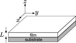
Figure 1: Schematic of a topological insulator film grown on substrate. The grown direction is defined as $z$ axis. The thickness of the film is $L$.

As shown in Fig. 1, we will consider a thin film grown along $z$ direction. The thickness of the film is $L$. We assume translational symmetry in $x$-$y$ plane so that the wave numbers $k_{x}$ and $k_{y}$ are good quantum numbers. We start with the effective model proposed to describe the bulk states near the $\Gamma$ point for the bulk Bi₂Se₃Zhang2009.natphys.5.438 . The states are mainly contributed by four hybridized states of Se and Bi $p_{z}$ orbitals, denoted as {$\left|p1_{z}^{+},\uparrow\right\rangle$, $\left|p2_{z}^{-},\uparrow\right\rangle$, $\left|p1_{z}^{+},\downarrow\right\rangle$, $\left|p2_{z}^{-},\downarrow\right\rangle\}$, where $+$ ($-$) stands for the even (odd) parity. The Hamiltonian is given by

$$H(\mathbf{k})=\epsilon_{0}(\mathbf{k})I_{4\times 4}+\left[\begin{array}[]{cccc}\mathcal{M}(\mathbf{k})&-iA_{1}\partial_{z}&0&A_{2}k_{-}\\ -iA_{1}\partial_{z}&-\mathcal{M}(\mathbf{k})&A_{2}k_{-}&0\\ 0&A_{2}k_{+}&\mathcal{M}(\mathbf{k})&iA_{1}\partial_{z}\\ A_{2}k_{+}&0&iA_{1}\partial_{z}&-\mathcal{M}(\mathbf{k})\end{array}\right],$$ (1)

where $k_{\pm}=k_{x}\pm ik_{y}$, $\epsilon_{0}(\mathbf{k})=C-D_{1}\partial_{z}^{2}+D_{2}k^{2}$, $\mathcal{M}(\mathbf{k})=M+B_{1}\partial_{z}^{2}-B_{2}k^{2}$, and $k^{2}=k_{x}^{2}+k_{y}^{2}$, with $A_{1}$, $A_{2}$, $B_{1}$, $B_{2}$, $C$, $D_{1}$, $D_{2}$, and $M$ the model parameters. This model has the time reversal symmetry and the inversion symmetry. Though we start with a concrete model, the conclusion in this paper should be applicable to other topological insulator films. We shall demonstrate that this model for the bulk states can produce the surface states with appropriate boundary condition.

II.2 General solutions of the surface states

Following the method by Zhou et al.Zhou2008.prl.101.246807 , the general solution for either the bulk states or the surface states can be derived analytically. Despite the existence of time-reversal symmetry, the $A_{2}k_{\pm}$ term couples opposite spins in Hamiltonian (1), and one has to solve a $4\times 4$ matrix, instead of the simplified $2\times 2$ one in the 2D caseZhou2008.prl.101.246807 . By putting a four-component trial solution

$$\psi=\psi_{\lambda}e^{\lambda z}$$ (2)

into the Schrödinger equation ($E$ is the eigenvalue of energy)

$$H(k,-i\partial_{z})\psi=E\psi,$$ (3)

the secular equation

$$\det\left|H(k,-i\lambda)-E\right|=0$$ (4)

gives four solutions of $\lambda(E)$, denoted as $\beta\lambda_{\alpha}(E)$, with $\alpha\in\{1,2\}$, $\beta\in\{+,-\}$, and

$$\lambda_{\alpha}(E)=\left[-\frac{F}{2D_{+}D_{-}}+(-1)^{\alpha-1}\frac{\sqrt{R}}{2D_{+}D_{-}}\right]^{\frac{1}{2}},$$ (5)

where for convenience we have defined

$$F = A_{1}^{2}+D_{+}(E-L_{1})+D_{-}(E-L_{2}),$$

$$R = F^{2}-4D_{+}D_{-}[(E-L_{1})(E-L_{2})-A_{2}^{2}k_{+}k_{-}],$$

$$D_{\pm} = D_{1}\pm B_{1},$$

$$L_{1} = C+M+(D_{2}-B_{2})k^{2},$$

$$L_{2} = C-M+(D_{2}+B_{2})k^{2}.$$ (6)

Because of double degeneracy, each of the four $\beta\lambda_{\alpha}(E)$ corresponds to two linearly independent four-component vectors, found as

$$\psi_{\alpha\beta 1} = \left[\begin{array}[]{c}D_{+}\lambda_{\alpha}^{2}-L_{2}+E\\ -iA_{1}(\beta\lambda_{\alpha})\\ 0\\ A_{2}k_{+}\end{array}\right],$$ (11)

$$\psi_{\alpha\beta 2} = \left[\begin{array}[]{c}A_{2}k_{-}\\ 0\\ iA_{1}(\beta\lambda_{\alpha})\\ D_{-}\lambda_{\alpha}^{2}-L_{1}+E\end{array}\right].$$ (16)

The general solution should be a linear combination of these eight functions

$$\Psi(E,k,z)=\sum_{\alpha=1,2}\sum_{\beta=\pm}\sum_{\gamma=1,2}C_{\alpha\beta\gamma}\psi_{\alpha\beta\gamma}e^{\beta\lambda_{\alpha}z},$$ (17)

with the superposition coefficients $C_{\alpha\beta\gamma}$ to be determined by boundary conditions. In the following, we will consider two different boundary conditions: one is semi-infinite focusing on only one surface at $z=0$; the other includes two opposite surfaces at $z=\pm L/2$. In both cases we assume open boundary conditions ($\Psi=0$) for the surface states at the surfaces.

II.3 Solutions for the surface states with semi-infinite boundary conditions

The surface states have a finite distribution near the boundary. For a film thick enough that the states at opposite surfaces barely couple to each other, we can focus on just one surface. Without loss of generality, we study a system from $z=0$ to $+\infty$. The boundary condition is given as

$$\Psi(z=0)=0\ \mathrm{and}\ \Psi(z\rightarrow+\infty)=0.$$ (18)

The condition of $\Psi(z\rightarrow+\infty)=0$ requires that $\Psi$ contains only the four terms in which $\beta=-$ and the real part of $\lambda_{\alpha}$ is positive.

Applying the boundary conditions of Eq. (18) to the general solution of Eq. (17), the secular equation of the nontrivial solution to the coefficients $C_{\alpha\beta\gamma}$ leads to

$$(\lambda_{1}+\lambda_{2})^{2}=-\frac{A_{1}^{2}}{D_{+}D_{-}},$$ (19)

which along with Eq. (5) gives the dispersion of the surface states

$$E_{\pm}=C+\frac{D_{1}M}{B_{1}}\pm A_{2}\sqrt{1-(\frac{D_{1}}{B_{1}})^{2}}k+(D_{2}-\frac{B_{2}D_{1}}{B_{1}})k^{2}.$$ (20)

Near the $\Gamma$ point, the dispersion shows a massless Dirac cone in $k$ space, with the Fermi velocity $v_{\mathrm{F}}=(A_{2}/\hbar)\sqrt{1-(\frac{D_{1}}{B_{1}})^{2}}$, instead of plain $A_{2}/\hbar$ as in Ref. Zhang2009.natphys.5.438 .

The wave functions for $E_{\pm}$ are found as

$$\Psi_{+} = C_{+}^{0}\left[\begin{array}[]{c}\frac{i}{2}\sqrt{\frac{D_{+}}{B_{1}}}\\ -\frac{1}{2}\sqrt{\frac{-D_{-}}{B_{1}}}\\ -\frac{1}{2}\sqrt{\frac{D_{+}}{B_{1}}}e^{i\varphi}\\ \frac{i}{2}\sqrt{\frac{-D_{-}}{B_{1}}}e^{i\varphi}\end{array}\right](e^{-\lambda_{2}^{+}z}-e^{-\lambda_{1}^{+}z}),$$ (25)

$$\Psi_{-} = C_{-}^{0}\left[\begin{array}[]{c}-\frac{i}{2}\sqrt{\frac{D_{+}}{B_{1}}}\\ \frac{1}{2}\sqrt{\frac{-D_{-}}{B_{1}}}\\ -\frac{1}{2}\sqrt{\frac{D_{+}}{B_{1}}}e^{i\varphi}\\ \frac{i}{2}\sqrt{\frac{-D_{-}}{B_{1}}}e^{i\varphi}\end{array}\right](e^{-\lambda_{2}^{-}z}-e^{-\lambda_{1}^{-}z}),$$ (30)

where $\lambda_{\alpha}^{\pm}$ are short for $\lambda_{\alpha}(E=E_{\pm})$ according to Eq. (5), $\tan\varphi\equiv k_{y}/k_{x}$, and $C_{\pm}^{0}$ are the normalization factors. The properties of the solution to $\lambda_{\alpha}$ determine the spatial distribution of the wave functions. Generally speaking, the edge states exist if $\lambda_{1}$ and $\lambda_{2}$ are both real or complex conjugate partners. For either case, there should be inequality relations

$$\frac{M}{B_{1}} > 0,$$

$$D_{+}D_{-} < 0\ .$$ (31)

The edge states distribute mostly near the surface ($z=0$), with the scale of the decay length about $\lambda_{1,2}^{-1}$ for real $\lambda_{1,2}$ or $[\mathrm{Re}(\lambda_{1,2})]^{-1}$ for complex $\lambda_{1,2}$. In the former case, the wavefunctions decay exponentially and monotonously away from the surface (not from $z=0$); while in latter case the decaying is accompanied by a periodical oscillation, which can be easily seen from the wavefunctions in Eq. (25). In addition, there exist complex solutions to $\lambda_{\alpha}$ when

$$\frac{A_{1}^{2}}{-D_{+}D_{-}}<\frac{4M}{B_{1}}.$$ (32)

II.4 Solutions for finite-thickness boundary conditions

When the thickness of the film is comparable with the characteristic length $1/\lambda_{1,2}$ of the surface states, there is coupling between the states on opposite surfaces. One has to consider the boundary conditions at both surfaces simultaneously. Without loss of generality, we will consider the top surface is located at $z=L/2$ and the bottom surface at $-L/2$. The boundary conditions are given as

$$\Psi(z=\pm\frac{L}{2})=0.$$ (33)

In this case, the general solution consists of all eight linearly independent functions. Applying the boundary conditions in Eq. (33) to the general solution of Eq. (17), the secular equation of the nontrivial solution to the superposition coefficients $C_{\alpha\beta\gamma}$ leads to a transcendental equation

$$\frac{\frac{D_{+}D_{-}}{A_{1}^{2}}(\lambda_{1}^{2}-\lambda_{2}^{2})^{2}+(\lambda_{1}^{2}+\lambda_{2}^{2})}{\lambda_{1}\lambda_{2}}=\frac{\tanh\frac{\lambda_{2}L}{2}}{\tanh\frac{\lambda_{1}L}{2}}+\frac{\tanh\frac{\lambda_{1}L}{2}}{\tanh\frac{\lambda_{2}L}{2}}.$$ (34)

In a large $L$ limit, $\tanh\frac{\lambda_{\alpha}L}{2}$ reduces to $1$ , then Eq. (34) can recover the result in Eq. (19). With the help of Eq. (5), Eq. (34) can be used to identify the energy spectra and the values of $\lambda_{\alpha}$ numerically.

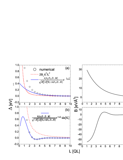
Figure 2: (Color online) [(a)(b)] The energy gap $\Delta\equiv E_{+}-E_{-}$ and [(c)(d)] the model parameter $B$ [defined in Eq. (III.2)] as functions of the film thickness $L$. Circles correspond to the numerical results of the transcendental equations (47) and (48). Solid and dash lines correspond to the approximate formulas to $\Delta$ when $L$ is finite [Eqs. (35) and (36)] or very small [Eq. (85)], respectively. All the parameters are adopted (a) by fitting experimental results of 4QL Bi₂Se₃, and (b) from the numerical fitting for the first principles calculation of Bi₂Se₃Zhang2009.natphys.5.438 , as listed in Tab. 1.

Due to the finite size effectZhou2008.prl.101.246807 , the coupling between the states at the top and bottom surfaces will open an energy gapLu2009.arxiv ; Liu2009.arxiv ; Linder2009.prb.80.205401 . We define the gap as $\Delta=E_{+}-E_{-}$ at the $\Gamma$ point, where $E_{+}$ and $E_{-}$ are two solutions of Eq. (34). For $\lambda_{\alpha}L\gg 1$ and $\lambda_{2}\gg\lambda_{1}$ ($L$ can be finite), the approximate expression for $\Delta$ can be found. If $\lambda_{\alpha}$ is real, the gap can be approximated by

$$\Delta\simeq\frac{4|A_{1}D_{+}D_{-}M|}{\sqrt{B_{1}^{3}(A_{1}^{2}B_{1}+4D_{+}D_{-}M)}}e^{-\lambda_{1}L},$$ (35)

which decays exponentially as a function of $L$. Fig. 2(a) shows the gap as a function of thickness, in which a set of model parameters used to fit the ARPES of 4QL Bi₂Se₃ thin film is employed, as listed in the first row of Tab. 1.

Table 1: Two sets of parameters for the 3D Dirac model. The first row is extracted from our effective model parameters for 4QL Bi₂Se₃ film in table 2, and the second row is adopted from the first principles calculationZhang2009.natphys.5.438 .

$M$	$A_{1}$	$A_{2}$	$B_{1}$	$B_{2}$	$C$	$D_{1}$	$D_{2}$
(eV)	(eVÅ)	(eVÅ)	(eVÅ2)	(eVÅ2)	(eV)	(eVÅ2)	(eVÅ2)
0.28	3.3	4.1	1.5	-54.1	-0.0068	1.2	-30.1
0.28	2.2	4.1	10	56.6	-0.0068	1.3	19.6

For some other materials there may exist complex $\lambda_{1}=\lambda_{2}^{\ast}$ and we can define $\lambda_{1}=a-ib$ and $\lambda_{2}=a+ib$, where $a>0$, $b>0$ according to Eq. (5). In this case, the gap is found as

$$\Delta\simeq\frac{8|A_{1}D_{+}D_{-}M|}{\sqrt{-B_{1}^{3}(A_{1}^{2}B_{1}+4D_{+}D_{-}M)}}e^{-aL}\sin(bL),$$ (36)

with

$$a \backsimeq \frac{A_{1}}{2\sqrt{-D_{+}D_{-}}},$$ (37)

$$b \backsimeq \sqrt{\frac{M}{B_{1}}+\frac{A_{1}^{2}}{4D_{+}D_{-}}}.$$ (38)

According to this result, the oscillation period of the gap $\pi/b$ becomes $\pi\sqrt{B_{1}/M}$ when $A_{1}=0$, in accordance with the result obtained by Liu et alLiu2009.arxiv . Fig. 2(b) shows the gap oscillation by using the model parameters listed in the second entry of Tab. 1. Besides, the sine function implies that $\Delta$ may be negative. Later we will see that the sign of $\Delta$ can be found by solving $E_{+}^{0}$ and $E_{-}^{0}$ from Eqs. (47) and (48), respectively.

III Effective continuous models

The solutions of the surface states and thin film of 3DTI can be applied to calculate physical properties explicitly. For instance, we can see whether the ground state of a thin film exhibits QSHE or not by calculating the Chern number or Z₂ invariant. It is also desirable to establish an effective continuous model to explore the properties of these surface states especially when other interactions have to be taken into account. For this purpose, in this section we derive an effective low-energy and continuous models for the surface states and thin film of 3DTI.

Due to the low-energy long-wavelength nature of the Dirac cone of the surface electrons, we can use the solutions of the surface states at the $\Gamma$ point as a basis to expand the Hamiltonian $H(k)$ in Eq.(1), which will be valid when the energy is limited within the band gap between the conduction and valence bands. This is equivalent to a truncation approximation as we exclude the solutions for the bulk states in the basis. In this approach, the Hamiltonian in Eq. (1) can be expressed as

$$H(\vec{k})=H_{0}(k=0)+\Delta H,$$ (39)

where

$$H_{0}=\left[\begin{array}[]{cc}h(A_{1})&0\\ 0&h(-A_{1})\end{array}\right],$$ (40)

with

$$h(A_{1})=\left[\begin{array}[]{cc}-D_{-}\partial_{z}^{2}+C+M&-iA_{1}\partial_{z}\\ -iA_{1}\partial_{z}&-D_{+}\partial_{z}^{2}+C-M\end{array}\right],$$ (41)

and

$$\Delta H=\left[\begin{array}[]{cc}D_{2}k^{2}-B_{2}k^{2}\sigma_{z}&A_{2}k_{-}\sigma_{x}\\ A_{2}k_{+}\sigma_{x}&D_{2}k^{2}-B_{2}k^{2}\sigma_{z}\end{array}\right].$$ (42)

The first term can be solved exactly, and the last term describes the behaviors of electrons near the $\Gamma$ point.

III.1 Basis states at $\Gamma$ point

$H_{0}$ in Eq. (40) is block-diagonal. Its solution can be found by solving each block separately, i.e., $h(A_{1})\Psi_{\uparrow}=E\Psi_{\uparrow}$ and $h(-A_{1})\Psi_{\downarrow}=E\Psi_{\downarrow}$. Because the lower block is the ”time” reversal of the upper block, the solutions satisfy $\Psi_{\downarrow}(z)=\Theta\Psi_{\uparrow}(z)$, where $\Theta=-i\sigma_{y}\mathcal{K}$ is the time-reversal operator, with $\sigma_{y}$ the $y$ component of the Pauli matrices and $\mathcal{K}$ the complex conjugation operation. Equivalently, we can replace $A_{1}$ by $-A_{1}$ in all the results for the upper block, to obtain those for the lower block. Therefore, we only need to solve $h(A_{1})$. Following the same approach in Sec. II, we put a two-component trial solution

$$\psi^{\uparrow}=\psi_{\lambda}^{\uparrow}e^{\lambda z}$$ (43)

into

$$h(A_{1},-i\partial_{z})\psi^{\uparrow}=E\psi^{\uparrow},$$ (44)

the secular equation for a nontrivial solution yields four roots of $\lambda(E)$, denoted as $\beta\lambda_{\alpha}$, with $\beta\in\{+,-\}$ and $a\in\{1,2\}$. Note that here $\lambda_{\alpha}$ is short for $\lambda_{\alpha}(k=0)$ in Eq. (5 ). Each $\beta\lambda_{\alpha}$ corresponds to a two-component vector

$$\psi_{\alpha\beta}^{\uparrow}=\left[\begin{array}[]{c}D_{+}\lambda_{\alpha}^{2}-l_{2}+E\\ -iA_{1}(\beta\lambda_{\alpha})\end{array}\right].$$ (45)

The general solution is a linear combination of the four linearly independent two-component vectors

$$\Psi_{\uparrow}=\sum_{\alpha=1,2}\sum_{\beta=+,-}C_{\alpha\beta}\psi_{\alpha\beta}^{\uparrow}e^{\beta\lambda_{\alpha}z}.$$ (46)

Applying the boundary conditions Eq. (33) to this general solution, we obtain two transcendental equations,

$$\frac{(C-M-E-D_{+}\lambda_{1}^{2})\lambda_{2}}{(C-M-E-D_{+}\lambda_{2}^{2})\lambda_{1}}=\frac{\tanh(\frac{\lambda_{2}L}{2})}{\tanh(\frac{\lambda_{1}L}{2})},$$ (47)

and

$$\frac{(C-M-E-D_{+}\lambda_{1}^{2})\lambda_{2}}{(C-M-E-D_{+}\lambda_{2}^{2})\lambda_{1}}=\frac{\tanh(\frac{\lambda_{1}L}{2})}{\tanh(\frac{\lambda_{2}L}{2})}.$$ (48)

The solutions to Eqs. (47) and (48) give two energies at the $\Gamma$ point, designated as $E_{+}^{0}\equiv E_{+}(k=0)$ and $E_{-}^{0}\equiv E_{-}(k=0)$, respectively. The eigen wavefunctions for $E_{+}^{0}$ and $E_{-}^{0}$ are, respectively,

$$\varphi(A_{1}) \equiv \Psi_{\uparrow}^{+}=C_{+}\left[\begin{array}[]{c}-D_{+}\eta_{1}^{+}f_{-}^{+}\\ iA_{1}f_{+}^{+}\end{array}\right],$$ (51)

$$\chi(A_{1}) \equiv \Psi_{\uparrow}^{-}=C_{-}\left[\begin{array}[]{c}-D_{+}\eta_{2}^{-}f_{+}^{-}\\ iA_{1}f_{-}^{-}\end{array}\right],$$ (54)

where $C_{\pm}$ are the normalization factors. The superscripts of $f_{\pm}^{\pm}$ and $\eta_{1,2}^{\pm}$ stand for $E_{\pm}^{0}$, and the subscripts of $f_{\pm}^{\pm}$ for parity, respectively. The expressions for $f_{\pm}^{\pm}$ and $\eta_{1,2}^{\pm}$ are given by

$$f_{+}^{\pm}(z) = \left.\frac{\cosh(\lambda_{1}z)}{\cosh(\frac{\lambda_{1}L}{2})}-\frac{\cosh(\lambda_{2}z)}{\cosh(\frac{\lambda_{2}L}{2})}\right|_{E=E_{\pm}^{0}},$$ (55)

$$f_{-}^{\pm}(z) = \left.\frac{\sinh(\lambda_{1}z)}{\sinh(\frac{\lambda_{1}L}{2})}-\frac{\sinh(\lambda_{2}z)}{\sinh(\frac{\lambda_{2}L}{2})}\right|_{E=E_{\pm}^{0}},$$ (56)

$$\eta_{1}^{\pm} = \left.\frac{(\lambda_{1})^{2}-(\lambda_{2})^{2}}{\lambda_{1}\coth(\frac{\lambda_{1}L}{2})-\lambda_{2}\coth(\frac{\lambda_{2}L}{2})}\right|_{E=E_{\pm}^{0}},$$ (57)

$$\eta_{2}^{\pm} = \left.\frac{(\lambda_{1})^{2}-(\lambda_{2})^{2}}{\lambda_{1}\tanh(\frac{\lambda_{1}L}{2})-\lambda_{2}\tanh(\frac{\lambda_{2}L}{2})}\right|_{E=E_{\pm}^{0}}.$$ (58)

The energy spectra and wavefunctions of the lower block $h(-A_{1})$ of $H_{0}$ can be obtained directly by replacing $A_{1}$ by $-A_{1}$. Based on the above discussions, the four eigenstates of $H_{0}$ can be given by

$$\Phi_{1} = \left[\begin{array}[]{c}\varphi(A_{1})\\ 0\end{array}\right],\ \Phi_{2}=\left[\begin{array}[]{c}\chi(A_{1})\\ 0\end{array}\right],$$ (63)

$$\Phi_{3} = \left[\begin{array}[]{c}0\\ \varphi(-A_{1})\end{array}\right],\ \Phi_{4}=\left[\begin{array}[]{c}0\\ \chi(-A_{1})\end{array}\right],$$ (68)

with $\Phi_{1}\rightarrow\Phi_{3}$ and $\Phi_{2}\rightarrow\Phi_{4}$ under the time-reversal operation. We should emphasize that these four solutions are for the surface states, and the solutions for the bulk states are not presented here. We use the four states as the basis states, and other states are discarded (except that in Fig. 3 where four extra bulk states are also included by the same approach), because of a large gap between the valence and conduction bands.

III.2 Effective model for 3DTI films

With the help of the four states Eq. (63) at the $\Gamma$ point, we can expand Hamiltonian Eq. (1) to obtain a new effective Hamiltonian

$$H_{\mathrm{eff}}\equiv\int_{-L/2}^{L/2}dz[\Phi_{1},\Phi_{4},\Phi_{2},\Phi_{3}]^{{\dagger}}H[\Phi_{1},\Phi_{4},\Phi_{2},\Phi_{3}],$$ (69)

where for convenience, we organize the sequence of the basis states following $\{\Phi_{1}$, $\Phi_{4}$, $\Phi_{2}$, $\Phi_{3}\}$. Under the reorganized basis, the effective Hamiltonian is found as

$$H_{\mathrm{eff}}=\left[\begin{array}[]{cc}h_{+}&0\\ 0&h_{-}\end{array}\right],$$ (70)

with

$$h_{+} = E_{0}-Dk^{2}+\left[\begin{array}[]{cc}\frac{\Delta}{2}-Bk^{2}&\tilde{A}_{2}k_{-}\\ \tilde{A}_{2}^{\ast}k_{+}&-\frac{\Delta}{2}+Bk^{2}\end{array}\right],$$ (73)

$$h_{-} = E_{0}-Dk^{2}+\left[\begin{array}[]{cc}-\frac{\Delta}{2}+Bk^{2}&-\tilde{A}_{2}^{\ast}k_{-}\\ -\tilde{A}_{2}k_{+}&\frac{\Delta}{2}-Bk^{2}\end{array}\right],$$ (76)

and

$$B = \frac{\tilde{B}_{1}-\tilde{B}_{2}}{2},\ \ D=\frac{\tilde{B}_{1}+\tilde{B}_{2}}{2}-D_{2},$$

$$E_{0} = (E_{+}+E_{-})/2,\ \ \Delta=E_{+}-E_{-},$$

$$\tilde{B}_{1} = B_{2}\langle\varphi(A_{1})|\sigma_{z}|\varphi(A_{1})\rangle,$$

$$\tilde{B}_{2} = B_{2}\langle\chi(A_{1})|\sigma_{z}|\chi(A_{1})\rangle,$$

$$\tilde{A}_{2} = A_{2}\langle\varphi(A_{1})|\sigma_{x}|\chi(-A_{1})\rangle.$$ (77)

We find that $\tilde{A}_{2}$ here can be either real or purely imaginary (see Appendix VII for details), classifying the model into two cases:

Case I is for a real $\tilde{A}_{2}\equiv\hbar v_{\mathrm{F}}$, and the effective Hamiltonian is further written as

$$h_{\tau_{z}}=E_{0}-Dk^{2}+\hbar v_{\mathrm{F}}\tau_{z}\vec{\sigma}\cdot\vec{k}+\tau_{z}\sigma_{z}(\frac{\Delta}{2}-Bk^{2}),\ \ \mathrm{(case\ I)};\\$$ (78)

and case II for a purely imaginary $\tilde{A}_{2}\equiv i\hbar v_{\mathrm{F}}$,

$$h_{\tau_{z}}=E_{0}-Dk^{2}+\hbar v_{\mathrm{F}}(\vec{\sigma}\times\vec{k})_{z}+\tau_{z}\sigma_{z}(\frac{\Delta}{2}-Bk^{2}),\ \ \mathrm{(case\ II)}$$ (79)

with $\tau_{z}=\pm 1$ corresponding to the upper (lower) $2\times 2$ block in Eq. (70), $v_{\mathrm{F}}$ the defined Fermi velocity and $\vec{\sigma}$ and $\vec{k}$ here only refer to the components in $x$-$y$ plane. In fact, these two effective Hamiltonian can consist of the invariants of the irreducible representation $D_{1/2}$ of SU(2) groupWinkler .

Eq. (73) can also be expressed in terms of the Pauli matrices

$$h_{\tau_{z}}=E_{0}-Dk^{2}+\mathbf{d}\cdot\mathbf{\sigma},$$ (80)

with

$$\mathbf{d}=\left\{\begin{array}[]{ll}\tau_{z}(\hbar v_{\mathrm{F}}k_{x},\ \hbar v_{\mathrm{F}}k_{y},\ \frac{\Delta}{2}-Bk^{2}),&\mathrm{(case\ I)}\\ &\\ (\hbar v_{\mathrm{F}}k_{y},\ -\hbar v_{\mathrm{F}}k_{x},\ \tau_{z}(\frac{\Delta}{2}-Bk^{2})).&\mathrm{(case\ II)}\end{array}\right.$$ (81)

$\mathbf{d}(k)$ vectors in case I and case II, respectively, correspond to Dresselhaus- and Rashba-like textures. Note that case I is essentially the effective 4$\times$4 model for the CdTe/HgTe quantum wellsBernevig2006.science.314.1757 . However, we find that case I only occurs for quite a small range of thickness. For most thicknesses of interest, $\tilde{A}_{2}$ is pure imaginary. Therefore, we only focus on case II in the following discussions. By far, we have reduced the anisotropic 3D Dirac model into a generalized effective model for 2D thin films, under the freestanding open boundary conditions.

III.3 Effective continuous model for surface states

Despite the simple explicit form, the parameters in Hamiltonian (70) need to be determined numerically. Before that, we can take two limits to see their behaviors. The first limit is $\lambda_{\alpha}L\gg 1$, for $\alpha=1,2$. In this case, $\tanh(\frac{\lambda_{\alpha}L}{2})\backsimeq 1$, and both Eqs. (47) and (48) reduce to

$$(C-M-E-D_{+}\lambda_{1}^{2})\lambda_{2}=(C-M-E-D_{+}\lambda_{2}^{2})\lambda_{1}.$$ (82)

Solving this equation, we have an effective continuous model for the surface states (ss) of 3D topological insulator as

$$H_{\mathrm{ss}} = C+\frac{D_{1}M}{B_{1}}+(D_{2}-B_{2}\frac{D_{1}}{B_{1}})k^{2}$$ (83)

$$+A_{2}\sqrt{1-(\frac{D_{1}}{B_{1}})^{2}}(\sigma_{x}k_{y}-\sigma_{y}k_{x}),$$

which has the same dispersion as Eq. (20) and the same Fermi velocity $v_{\mathrm{F}}=\frac{A_{2}}{\hbar}\sqrt{1-(\frac{D_{1}}{B_{1}})^{2}}$ as for the semi-infinite boundary conditions. In an isotropic case, $D_{1}=D_{2}$ and $B_{1}=B_{2}$, the quadratic term disappears and we have a linear dispersion for the Dirac cone. Finally it is noticed that the models for the surface states at the top and bottom surface have the same form assumed $\lambda_{\alpha}L\gg 1.$ We will see that these results work well even for films down to five quintuple layers (QL) of atoms in thickness (1 QL is about 1 nm).

III.4 The ultra-thin limit

Another opposite limit is $L\rightarrow 0$, which is a little bit complicated since $\lambda_{\alpha}L$ does not approach to zero when $L$ is very small. In Eq. (47), the left side has an order of $L^{2}$ when $L\rightarrow 0$, so $\tanh(\frac{\lambda_{1}L}{2})$ must have the order of $L^{-2}$, which means

$$\tanh(\frac{\lambda_{1}L}{2})=0\Rightarrow\lambda_{1}=i\frac{\pi}{L}.$$ (84)

Combining this result with Eq. (5), the model becomes

$$h_{\tau_{z}}=\frac{D_{1}\pi^{2}}{L^{2}}+D_{2}k^{2}+A_{2}(\vec{\sigma}\times\vec{k})_{z}+\tau_{z}(\frac{B_{1}\pi^{2}}{L^{2}}+B_{2}k^{2})\sigma_{z}.$$ (85)

It is found that a finite energy gap opens at $k=0$, i.e., $\Delta=2B_{1}\pi^{2}/L^{2}$ as shown in Fig. 2. Note that this result in the $L\rightarrow 0$ limit even provides a rough estimate of the gap for most thicknesses. Besides, the continuum limit generally assumed in this work also works well even for only several quintuple layers.

IV Structure Inversion Asymmetry

IV.1 Structure Inversion Asymmetry

A recent experimentZhang2009.arXiv.0911.3706 revealed that the substrate on which the film is grown influences dramatically electronic structure inside the film. Because the top surface of the film is usually exposed to the vacuum and the bottom surface is attached to a substrate, the inversion symmetry does not hold along $z$ direction, leading to the Rashba-like energy spectra for the gapped surface states. In this case, an extra term that describes the structure inversion asymmetry (SIA) needs to be taken into account in the effective model.

We use the same method as that in Sec. III to include the SIA term. Without loss of generality, we add a potential energy $V(z)$ into the Hamiltonian. Generally speaking, $V(z)$ can be expressed as $V(z)=V_{s}(z)+V_{a}(z)$, in which $V_{s}(z)=V_{s}(-z)$ and $V_{a}(z)=-V_{a}(-z)$. The symmetric term $V_{s}$ could contribute to the mass term $\Delta$ in the effective model, which may lead to an energy splitting of the Dirac cone at the $\Gamma$ point. We do not discuss it in details in this paper. Here we focus on the case of the antisymmetric term, $V(z)=V_{a}(z)$, which breaks the top-bottom inversion symmetry in the Hamiltonian. A detailed analysis demonstrates that $V_{a}(z)$ couples $\Phi_{1}$ $(\Phi_{3})$ to $\Phi_{2}$ $(\Phi_{4})$, which can be readily seen according to their spin and parity natures. The modified effective Hamiltonian in the presence of $V(z)$ becomes

$$H_{\mathrm{eff}}^{\mathrm{SIA}}=H_{\mathrm{eff}}+\left[\begin{array}[]{cccc}0&0&\tilde{V}&0\\ 0&0&0&\tilde{V}^{\ast}\\ \tilde{V}^{\ast}&0&0&0\\ 0&\tilde{V}&0&0\end{array}\right],$$ (86)

where

$$\tilde{V}=\int_{-L/2}^{L/2}dz\langle\varphi(A_{1})|V_{a}(z)|\chi(A_{1})\rangle.$$ (87)

Comparing this definition with that of $\tilde{A}_{2}$ in Eq. (III.2), we find that $\tilde{V}$ also can be either real or purely imaginary. In the case of a purely imaginary (case II) $\tilde{A}_{2}$, $\tilde{V}$ must be real (see Appendix VII), and the effective Hamiltonian with SIA can be written as

$$H_{\mathrm{eff}}^{\mathrm{SIA}}=\left[\begin{array}[]{cc}h_{+}(k)&\tilde{V}\sigma_{0}\\ \tilde{V}\sigma_{0}&h_{-}(k)\end{array}\right].$$

In the case of a real $\tilde{A}_{2}$, $\tilde{V}$ must be purely imaginary, and the effective Hamiltonian with SIA then has the form

$$H_{\mathrm{eff}}^{\mathrm{SIA}}=\left[\begin{array}[]{cc}h_{+}(k)&\tilde{V}\sigma_{z}\\ -\tilde{V}\sigma_{z}&h_{-}(k)\end{array}\right].$$

Without the SIA term, the effective Hamiltonian (79) gives the energy spectra of the gapped surface states as

$$E_{\pm}=E_{0}-Dk^{2}\pm\sqrt{(\frac{\Delta}{2}-Bk^{2})^{2}+(\hbar v_{\mathrm{F}})^{2}k^{2}},$$ (88)

where $+$ $(-)$ sign stands for the conduction (valence) band, each of which has double spin degeneracy due to time-reversal symmetry. When the SIA term is included, the Hamiltonian (86) gives

$$E_{1,\pm} = E_{0}-Dk^{2}\pm\sqrt{(\frac{\Delta}{2}-Bk^{2})^{2}+(|\tilde{V}|+\hbar v_{\mathrm{F}}k)^{2}},$$

$$E_{2,\pm} = E_{0}-Dk^{2}\pm\sqrt{(\frac{\Delta}{2}-Bk^{2})^{2}+(|\tilde{V}|-\hbar v_{\mathrm{F}}k)^{2}},$$

where the extra index 1 (2) stands for the inner (outer) branches of the conduction or valence bands. The energy spectra in the presence of $\tilde{V}$ is shown in Fig. 3. Each spin-degenerate dispersion in Eq. (88) shifts away from each other along $k$ axis. Both the conduction and valence bands show Rashba-like splitting. An intuitive understanding of the energy spectra in Fig. 3 can be given with the help of Fig. 4. On the left is for a thicker freestanding symmetric TI film, and it has a single gapless Dirac cone on each of its two surfaces, with the solid and dash lines for the top and bottom surface, respectively. The two Dirac cones are degenerate. The top of Fig. 4 indicates that the inter-surface coupling across an ultrathin film will turn the Dirac cones into gapped Dirac hyperbolas. On the bottom of Fig. 4, SIA lifts the Dirac cone at the top surface while lowers the Dirac cone at the bottom surface. The potential difference at the top and bottom surfaces removes the degeneracy of the Dirac cones. On the right of Fig. 4, the coexistence of both the inter-surface coupling and SIA leads to two gapped Dirac hyperbolas which also split in $k$-direction, as shown in Fig. 3.

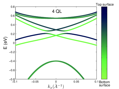
Figure 3: (Color online) Energy spectra of surface states (four branches in the middle) and several branches of bulk states (those at the top and the bottom) for a film with the thickness of 4 QL in the presence of the structure inversion asymmetry. The color of lines corresponds to the spatial distribution of the wavefunctions in $z$ direction. Dark blue (light green) represents that the wavefunctions mainly distribute on the side of the top (substrate) surface. The model parameters are listed in the first row of Table 1.

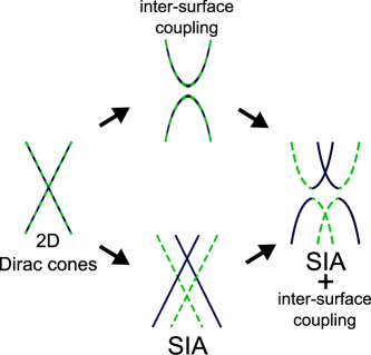
Figure 4: (Color online) The evolution of the doubly-degenerate gapless Dirac cones for the 2D surface states, in the presence of both the inter-surface coupling and structure inversion asymmetry, into the gapped hyperbolas that also split in $k$-direction. The blue solid and green dashed lines correspond to the states residing near the top and bottom surfaces, respectively.

IV.2 Location of the surface states

Location of the surface states can be revealed by evaluating the expectation of position z of these states. The spatial distributions along the z direction of a state $\psi_{\alpha}$ can be evaluated by the expectation of position in $z$ direction $\langle z\rangle$,

$$\langle z\rangle_{\alpha}=\int_{-\frac{L}{2}}^{\frac{L}{2}}z|\psi_{\alpha}|^{2}dz.$$ (90)

By this definition, $\langle z\rangle_{\alpha}\in[-\frac{L}{2},\frac{L}{2}]$ and $\langle z\rangle_{\alpha}$ becomes $0$ for a symmetric spatial distribution.

With the SIA, the eigen wavefunctions are found as

$$\psi_{1\pm}=\frac{1}{2\sqrt{E_{\pm}^{\mathrm{in}}(E_{\pm}^{\mathrm{in}}+t)}k}\left[\begin{array}[]{c}i(t+E_{\pm}^{\mathrm{in}})k\\ (|\tilde{V}|+\hbar v_{\mathrm{F}}k)k_{+}\\ i(|\tilde{V}|+\hbar v_{\mathrm{F}}k)k\\ (t+E_{\pm}^{\mathrm{in}})k_{+}\end{array}\right],$$ (91)

with $E_{\pm}^{\mathrm{in}}=E_{1\pm}-E_{0}+Dk^{2}$, $t=\frac{\Delta}{2}-Bk^{2}$, and,

$$\psi_{2\pm}=\frac{1}{2\sqrt{E_{\pm}^{\mathrm{out}}(E_{\pm}^{\mathrm{out}}+t)}k}\left[\begin{array}[]{c}-i(t+E_{\pm}^{\mathrm{out}})k\\ (|\tilde{V}|-\hbar v_{\mathrm{F}}k)k_{+}\\ i(-|\tilde{V}|+\hbar v_{\mathrm{F}}k)k\\ (t+E_{\pm}^{\mathrm{out}})k_{+}\end{array}\right]$$ (92)

with $E_{\pm}^{\mathrm{out}}=E_{2\pm}-E_{0}+Dk^{2}$. Fig. 3 demonstrates $\langle z\rangle$ by the brightness of lines, with dark blue for $\langle z\rangle=\frac{L}{2}$ (the top surface), and light green for $\langle z\rangle=-\frac{L}{2}$ (the substrate or bottom surface).

For a thin film of 4 quintuple layers (QL), $L=3.8$nm, it is found that the two surface states are well separated and dominantly distributed near the two surfaces. The averaged $\langle z\rangle\simeq\pm\frac{L}{3}$, which is about 2/3 of a QL ($\approx L/6$) deviating from the surface. In this case the top and bottom surface states are well defined even without the SIA ($\tilde{V}=0$). The average value remains almost unchanged in a large range of $k$. However, the crossing point of the spectra of the top and bottom surface states, the averaged $\langle z\rangle$ changes from $+L/3$ to 0, and then goes to the value of $-L/3$. This demonstrates that the finite thickness makes the two states couple with each other as their wave functions along the z direction have a finite overlap. As a result the two states open an energy gap as in the case of edge states in QSH systemZhou2008.prl.101.246807 . The value of the gap is a function of $L$ as shown in Fig. 2(a) and (b). Near this region, $\langle z\rangle$ varies from $\langle z\rangle\simeq L/3$ to $-L/3$, and becomes zero exactly when two states are mixed completely. For a large $L$, we find that the averaged distance of the surface states deviating from the surface remains about $1$ QL.

Simply speaking, the states close to the top surface are easier to be probed by light than those close to the bottom surface. This provides a hint to understand why there are branches in energy spectra with much more faint ARPES signalsZhang2009.arXiv.0911.3706 .

V Thin film B$\mathrm{i}_{2}$S$\mathrm{e}_{3}$ and QSH states

In this section, we will investigate the realization of QSH effect in thin films and apply the effective model to the thin film Bi₂Se₃. When the system does not break the inversion symmetry, the effective Hamiltonian is block-diagonalized by $\tau_{z}=\pm 1$. This is in a good agreement with the theory by Murakami et alMurakami2007.prb.76.205304 . In this case we can define a $\tau_{z}$ -dependent Chern number (Hall conductance) for each block like the spin Chern numberSheng.prl.97.036808 , from which the nontrivial QSH phase can be identified. After introducing the SIA term, the $\tau_{z}$-dependent Chern number loses its meaning as the two blocks are mixed together. However, we can still employ the Z₂ topological classificationKane2005.prl.95.146802 , which requires no inversion symmetry, to identify possible QSH thin films in experiment.

V.1 QSH effect without SIA

Considering the block-diagonal form of the effective model without SIA (70), we can derive the Hall conductance for each block, separately. For the $2\times 2$ Hamiltonian in terms of the $\mathbf{d}(k)$ vectors and Pauli matrices in Eq. (80), the Kubo formula for the Hall conductance can be generally expressed as Qi2006.prb.74.085308 ; Zhou2006.prb.73.165303

$$\sigma_{xy}=-\frac{e^{2}}{2\Omega\hbar}\sum_{k}\frac{(f_{k,-}-f_{k,+})}{d^{3}}\epsilon_{\alpha\beta\gamma}\frac{\partial d_{a}}{\partial k_{x}}\frac{\partial d_{\beta}}{\partial k_{y}}d_{\gamma}$$ (93)

where $\Omega$ is the volume of the system, $d$ the norm of $(d_{x},d_{y},d_{z})$, $f_{k,\pm}=$ $1/\{\exp[(E_{\pm}(k)-\mu)/k_{B}T]+1\}$ the Fermi distribution function of electron ($+$) and hole ($-$) bands, with $\mu$ the chemical potential, $k_{B}$ the Boltzmann constant, and $T$ the temperature.

At zero temperature and when the chemical potential $\mu$ lies between the band gap $(-\frac{|\Delta|}{2},\frac{|\Delta|}{2})$, the Fermi functions reduce to $f_{k,+}=0$ and $f_{k,-}=1$. In this case we haveLu2009.arxiv

$$\sigma_{xy}^{\tau_{z}}=-\tau_{z}\frac{e^{2}}{2h}[\mathrm{sgn}(\Delta)+\mathrm{sgn}(B)].$$ (94)

This result intuitively shows that only when $B$ and $\Delta$ have the same sign, the Chern number is equal to $+1$ or $-1$, which is topologically nontrivial, and the Hall conductance is quantized to be $\pm e^{2}/h$. In other words, the QSH depends not only on the sign of $\Delta$ at the $\Gamma$ point but also on that of $B$ for $k$ large enough. Experimentally, the $\tau_{z}$-dependent Hall conductance can be probed by the nonlocal measurement, just like that for the 2D CdTe/HgTe quantum wellsRoth2009.science.325.294 .

V.2 QSH effect with SIA: Z₂ invariant

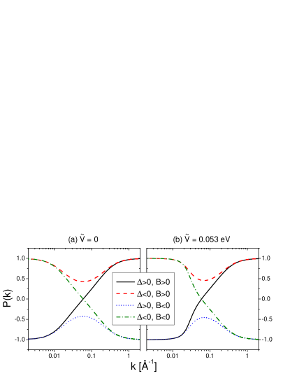
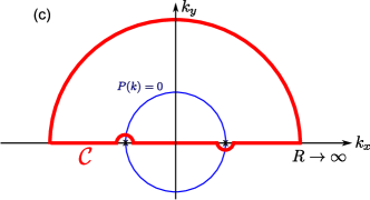
Figure 5: (Color online) [(a) and (b)] $P(k)$ for four combinations of $\Delta$ and $B$, in absence (a) and the presence (b) of a small SIA $\tilde{V}$. $|\Delta|$=0.07 eV and $|B|$=10 eV Ų. (c) The contour $\mathcal{C}$ is used to count the number of the pairs of the zeros of $P(k)$, which form a circle ring when $\Delta B>0$.

In the presence of SIA, $\tilde{V}$ couples the blocks $h_{+}$ and $h_{-}$, so the $\tau_{z}$-dependent Hall conductance becomes nonsense. Following Kane and MeleKane2005.prl.95.146802 , we can employ the Z₂ topological classification to give a criterion of the QSH phase, because it does not require inversion symmetry as a necessary condition. The Z₂ index can be obtained by counting the number of pairs of complex zeros of $P(\mathbf{k})\equiv\mathrm{Pf}[A(\mathbf{k})]$, where the Pfaffian is defined as

$$\mathrm{Pf}[A(\mathbf{k})]=\frac{1}{2^{n}n!}\sum_{\mathrm{\ Permutations}\newline \mathrm{of}\ \{i_{1},...,i_{2n}\}}(-1)^{N}A_{i_{1}i_{2}}...A_{i_{2n-1}i_{2n}},$$ (95)

in which $N$ counts the number of times of permutations, and $A(\mathbf{k})$ is a $2n$ order anti-symmetric matrix defined by the overlaps of time reversal

$$A_{ij}(\mathbf{k})=\langle u_{i}(\mathbf{k})|\Theta|u_{j}(\mathbf{k})\rangle$$ (96)

with $i,j$ run over all the bands below the Fermi surface, i.e., $\psi_{1-}$ and $\psi_{2-}$ in the present case according to Eqs. (91) and (92). Based on the spin nature of the basis states $\{\Phi_{1},\Phi_{4},\Phi_{2},\Phi_{3}\}$ in our effective model, the time-reversal operator here is defined as $\Theta\equiv i\sigma_{x}\otimes\sigma_{y}\mathcal{K}$, where $\sigma_{x}$ and $\sigma_{y}$ are the $x$- and $y$-component of Pauli matrices, respectively, and $\mathcal{K}$ the complex conjugate operator. The number of pairs of zeros can be counted by evaluating the winding of the phase of $P(\mathbf{k})$ around a contour $C$ enclosing half of the complex plane of $\mathbf{k}=k_{x}+ik_{y}$,

$$I=\frac{1}{2\pi i}\oint_{C}d\mathbf{k}\cdot\nabla_{\mathbf{k}}\mathrm{log}[P(\mathbf{k})+i\delta].$$ (97)

Because the model is isotropic, we can choose $\mathcal{C}$ to enclose the upper half plane, the integral then reduces to only the path along $k_{x}$ -axis while the part of the half-circle integral vanishes for $\delta>0$ and $\left|\mathbf{k}\right|\rightarrow+\infty$.

In the absence of the SIA term, $P(\mathbf{k})$ is found for the Hamiltonian (79) as

$$P(k)=\frac{-\frac{\Delta}{2}+Bk^{2}}{\sqrt{(\frac{\Delta}{2}-Bk^{2})^{2}+(\hbar v_{\mathrm{F}})^{2}k^{2}}},$$ (98)

in which one can check that the zero points exist only when $k^{2}=\Delta/2B>0$, and form a circle ring. Along $k_{x}$-axis only one of a pair of zeros in the ring is enclosed in the contour $\mathcal{C}$, which gives a $Z_{2}$ index $I=1$. This defines the nontrivial QSH phase, and is in consistence with the conclusion by the Hall conductance in Eq. (94).

In the presence of a small SIA term $\tilde{V}<\hbar v_{\mathrm{F}}\sqrt{|\Delta/2B|}$, with the help of the eigen wavefunctions (91) and (92), real $P(\mathbf{k})$ can be found (after a $U(1)$ rotation) as

$$P(k) = \frac{(t+E_{-}^{\mathrm{in}})(t+E_{-}^{\mathrm{out}})+|\tilde{V}|^{2}-(\hbar v_{\mathrm{F}}k)^{2}}{2\sqrt{E_{-}^{\mathrm{in}}E_{-}^{\mathrm{\ out}}(t+E_{-}^{\mathrm{in}})(t+E_{-}^{\mathrm{out}})}}$$ (101)

$$\times\left\{\begin{array}[]{cc}\mathrm{sgn}(\hbar v_{\mathrm{F}}k-|\tilde{V}|),&\Delta>0\\ 1,&\Delta\leq 0\end{array}\right.,$$

where the $\mathrm{sgn}$ is to secure the continuity of $P(\mathbf{k})$. One can check that $P(0)=-\mathrm{sgn}(\Delta)$ and $P(\infty)=\mathrm{sgn}(B)$ . Besides, for a small $\tilde{V}$, the behavior of $P(\mathbf{k})$ between $P(0)$ and $P(\infty)$ will not change qualitatively (see Fig. 5). Therefore, for $\Delta B>0$, $P(k_{x},0)$ should still have odd pairs of zeros. For a large $\tilde{V}\geq\hbar v_{\mathrm{F}}\sqrt{|\Delta/2B|}$,

$$P(k) = \frac{(t+E_{-}^{\mathrm{in}})(t+E_{-}^{\mathrm{out}})+|\tilde{V}|^{2}-(\hbar v_{\mathrm{F}}k)^{2}}{2\sqrt{E_{-}^{\mathrm{in}}E_{-}^{\mathrm{\ out}}(t+E_{-}^{\mathrm{in}})(t+E_{-}^{\mathrm{out}})}}$$ (104)

$$\times\left\{\begin{array}[]{ccc}\mathrm{sgn}(\hbar v_{\mathrm{F}}k-|\tilde{V}|),&B<0&\\ 1,&B\geq 0&\end{array}\right..$$

One can check for this case $P(0)P(\infty)$ is always positive thus $P(k)$ has even pairs of zeros, regardless of the signs and values of $\Delta$ and $B$. In other words, a large SIA will always destroy the quantum spin Hall phase.

V.3 Thin film Bi₂Se₃ and QSH effect

Table 2: Fitting parameters to the Bi₂Se₃ thin films, using the energy spectra Eq. (IV.1) from our effective model.[adopted from Ref. Zhang2009.arXiv.0911.3706 ]

Layers	$E_{0}$	$D$	$\Delta$	$B$	$v_{\mathrm{F}}$	$|\tilde{V}|$
(QL)	(eV)	(eVÅ2)	(eV)	(eVÅ2)	($10^{5}$m/s)	(eV)
2	-0.470	-14.4	0.252	21.8	4.47	0
3	-0.407	-9.7	0.138	18.0	4.58	0.038
4	-0.363	-8.0	0.070	10.0	4.25	0.053
5	-0.345	-15.3	0.041	5.0	4.30	0.057
6	-0.324	-13.0	0	0	4.28	0.068

Recently, thickness-dependent band structure of molecular beam epitaxy grown ultrathin films Bi₂Se₃ was investigated by in-situ angle-resolved photoemission spectroscopyZhang2009.arXiv.0911.3706 . An energy gap was first observed experimentally in the surface states of Bi₂Se₃ below the thickness of six quintuple layers, which confirms theoretical prediction as a finite size effectZhou2008.prl.101.246807 ; Lu2009.arxiv ; Liu2009.arxiv ; Linder2009.prb.80.205401 .

Table 2 shows the fitting parameters to the ARPES data of Bi₂Se₃ thin filmsZhang2009.arXiv.0911.3706 using the energy spectra formula [Eq. (IV.1)]. For the films with thickness ranging from 2 QL to 5 QL, all of them satisfy $\mathrm{sgn}(\Delta B)>0$ and $\tilde{V}<\hbar v_{\mathrm{F}}\sqrt{|\Delta/2B|}$, hence the films are possibly in the QSH regime. We identify that only 2 QL, 3 QL, and 4 QL belong to the nontrivial case for potential QSH effect. 5 QL is an exceptional case that the fitted parameters $B$ and $D$ do not satisfy the existence condition of an edge states solutionZhou2008.prl.101.246807 . The condition of $B^{2}<D^{2}$ will lead to the band gap closing for a large $k$. However, it is understood that the model is only valid near the $\Gamma$ point, and the fitting parameters are limited to the case of small $k$. And the band gap was measured clearly for the film of 5QL.

It was previously predicted, using the parameters from the first-principles calculationZhang2009.natphys.5.438 , that the gap $\Delta$ should oscillate as a function of the film thicknessLu2009.arxiv ; Liu2009.arxiv ; Linder2009.prb.80.205401 . However, this oscillation is not reflected in the measured results.

V.4 QSH effect of SIA and the edge states

In the quantum Hall effect the Chern number of the bulk states has an explicit correspondence to the number of edge states in an open boundary conditionHatsugai1993.prl.71.3697 . In topological insulator or QSH system, the Z₂ topological invariant has also a relation to the number of helical edge statesQi2006.prb.74.045125 . As a supplementary support to the above conclusion, we demonstrated the presence of edge states in a periodic boundary condition along the x-direction and an open boundary condition (say along y-direction) imposed in a geometry of strip of the thin film by means of numerical calculation. Using the parameters in Table I, we have concluded that a stripe of 2 - 4 QL will exhibit helical edge states. More specifically, we present the energy dispersion for 4QL in Fig. 6. There is a doubly-degenerate Dirac point inside the gap of the 2D surface states for 4 QL in consistence with the results obtained in the above sections.

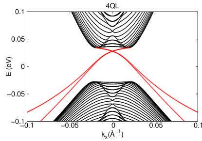
Figure 6: (Color online) The energy spectra by the tight binding calculation for 4 QL of Bi₂Se₃ thin films with the width along $y$-direction 200 nm. The parameters are given in table 2.

VI Conclusions

We derived two-dimensional effective continuous models for the surface states and thin films of three-dimensional topological insulators (3DTI). A gapless Dirac cone was confirmed for the surface states of a 3DTI. For a thin film, the coupling between opposite topological surface states in space opens an energy gap, and the Dirac cone evolves into a gapped Dirac hyperbola. The thin film may break the top-bottom symmetry. For example, the thin film grows on a substrate, and possesses the structural inversion asymmetry (SIA). This SIA leads to a Rashba-like coupling and energy splitting in the momentum space. It also leads to asymmetric distributions of states along film growth direction.

The ARPES measurements on Bi₂Se₃ films have demonstrated that the surface spectra opens a visible energy gap when the thickness is below 6QLs.Zhang2009.arXiv.0911.3706 The energy gap was observed to be a function of the thickness of thin film, and in a good consistence with theoretical prediction as a finite size effect of the thickness of thin film. The Rashba-like splitting was measured clearly in the thin film of 2 to 6 QLs. This can be explained very well from the inclusion of the SIA. Since the thin film was grown on a SiC substrate and the other surface is exposed to the vacuum this fact results in the SIA in the thin film. Another direct evidence to support the SIA is the signal intensity pattern of the energy spectra of ARPES. Usually the surface states are located dominantly near the top and bottom surfaces. The signal intensity for these two branches of energy spectra of ARPES are different. The SIA will cause the coupling between two surface states near their crossing point. That is why the Rashba-like splitting of the ARPES spectra has a bright crossing point near the $\Gamma$ point, with one branch bright and the other almost invisible. Thus the SIA term can be used to describe the ARPES measurements on the thin film Bi₂Se₃ very well.

Our effective model demonstrates that the 3DTI can be reduced to an two-dimensional quantum spin Hall system due to the spatial confinement. Strictly speaking, the system is no longer a 3DTI in the original sense once the energy gap opens in the surface bands, since the Z2 invariant for the bulk states becomes zero. However the surface bands themselves may contribute a non-trivial one in the Z2 invariant even when the SIA term is included. Our calculation demonstrates that a strong SIA always intends to destroy the quantum spin Hall effect. A critical value for SIA exists, at the point there is a transition from a topological trivial to non-trivial phases. Based on the model parameters fitted from the experimental data of ARPES, we conclude that the thin film Bi₂Se₃ should exhibit quantum spin Hall effect once the energy gap opens in the surface spectra due to the spatial confinement of the thin film.

VII Appendix: Model parameters $\tilde{A}_{2}$ and $\tilde{V}$

Table 3: Four possible combinations of $\lambda_{1}$ and $\lambda_{2}$, according to Eq. (5), and resulting $f_{\pm}$ and $\eta_{1,2}$ according to Eq. (63). According to Eq. (5), $\lambda_{1}^{2}<\lambda_{2}^{2}$, so there does not exist a case when $\lambda_{1}$ is real and $\lambda_{2}$ is pure imaginary.

	$\lambda_{1}$	$\lambda_{2}$	$f_{\pm}$	$\eta_{1,2}$
case A	$\lambda_{2}^{*}$	$\lambda_{1}^{*}$	imaginary	real
	real	real	real	real
case B	imaginary	real	real	real
	imaginary	imaginary	real	real

Table 4: Four possible groups of $E_{+}$ and $E_{-}$, and resulting values of $\tilde{A}_{2}$ and $\tilde{V}$.

$E_{+}$	$E_{-}$	$\widetilde{A}_{2}$	$\widetilde{V}$
case A	case A	imaginary	real
case A	case B	real	imaginary
case B	case A	real	imaginary
case B	case B	imaginary	real

In this appendix, we demonstrate that both the parameters $\tilde{A}_{2}$ and $\tilde{V}$ in the effective model (70) can be either real or purely imaginary, and the product of $\tilde{A}_{2}\tilde{V}$ must be pure imaginary. By putting the wavefunctions Eqs. (51) and (54) into the definitions in Eqs. (III.2) and (87), we have

$$\tilde{A}_{2} = iA_{1}A_{2}D_{+}C_{+}C_{-}\int_{-\frac{L}{2}}^{\frac{L}{2}}dz[\eta_{2}^{-}f_{+}^{+\ast}f_{+}^{-}+\eta_{1}^{+\ast}f_{-}^{+\ast}f_{-}^{-}]$$

$$\tilde{V} = C_{+}C_{-}\int_{-\frac{L}{2}}^{\frac{L}{2}}dzV(z)[D_{+}^{2}\eta_{1}^{+\ast}\eta_{2}^{-}f_{-}^{+\ast}f_{+}^{-}+A_{1}^{2}f_{+}^{+\ast}f_{-}^{-}].$$

For arbitrary energy, Eq. (5) requires that the values of $\lambda_{1}$ and $\lambda_{2}$ can only be one of the combinations shown in Tab. III. By putting these combinations into Eq. (55)-(58), one can show that for the first entry, $\eta_{1}$ and $\eta_{2}$ are real while $f_{+}$ and $f_{-}$ are pure imaginary, referred as the case A; while for entries 2 - 4, all of $\eta_{1}$, $\eta_{2}$, $f_{+}$, and $f_{-}$ are real, referred as the case B. For an arbitrary group of $E_{+}$ and $E_{-}$, each of them belongs to either the case A or B, leading to four possibilities, as shown in Tab. 4. In particular, according to Eq. (32), when $A_{1}^{2}/(-D_{+}D_{-})>4M/B_{1}$, there is no complex $\lambda_{1,2}$, corresponding to the last row of Tab. 4, i.e., $\tilde{A}_{2}$ is pure imaginary while $\tilde{V}$ is real.

References

References

- (1) For introductions to topological insulators, see Kane C L and Mele E J 2006 Science 314 1692; Zhang S C 2008 Physics 1 6; Buttiker M 2009 Science 325 278; Moore J 2009 Nat. Phys. 5 378.
- (2) Sarma S D and Pinczuk A 1997 Perspectives in Quantum Hall Effects (New York: Wiley)
- (3) Kane C L and Mele E J 2005 Phys. Rev. Lett. 95 226801
- (4) Kane C L and Mele E J 2005 Phys. Rev. Lett. 95 146802
- (5) Bernevig B A, Hughes T L and Zhang S 2006 Science 314 1757
- (6) Konig M, Wiedmann S, Brune C, Roth A, Buhmann H, Molenkamp L W, Qi X L and Zhang S C 2007 Science 318 766
- (7) Roth A, Brune C, Buhmann H, Molenkamp L W, Maciejko J, Qi X L and Zhang S C 2009 Science 325 294
- (8) Li J, Chu R L, Jain J K and Shen S Q 2009 Phys. Rev. Lett. 102 136806
- (9) Jiang H, Wang L, Sun Q F and Xie X C 2009 Phys. Rev. B 80 165316
- (10) Groth C W, Wimmer M, Akhmerov A R, Tworzydlo J and Beenakker C W J 2009 Phys. Rev. Lett. 103 196805
- (11) Fu L, Kane C L and Mele E J 2007 Phys. Rev. Lett. 98 106803
- (12) Moore J E and Balents L 2007 Phys. Rev. B 75 121306
- (13) Murakami S 2007 New J. Phys. 9 356
- (14) Teo J C Y, Fu L and Kane C L 2008 Phys. Rev. B 78 045426
- (15) Hsieh D, Qian D, Wray L, Xia Y, Hor Y S, Cava R J and Hasan M Z 2008 Nature 452 970
- (16) Hsieh D, Xia Y, Wray L, Qian D, Pal A, Dil J H, Osterwalder J, Meier F, Bihlmayer G, Kane C L et al 2009 Science 323 919
- (17) Xia Y, Qian D, Hsieh D, Wrayl L, Pal1 A, Lin H, Bansil A, Grauer D, Hor Y S, Cava R J et al 2009 Nat. Phys. 5 398
- (18) Chen Y L, Analytis J G, Chu J H, Liu Z K, Mo S K, Qi X L, Zhang H J, Lu D H, Dai X, Fang Z et al 2009 Science 325 178
- (19) Zhang H, Liu C X, Qi X L, Dai X, Fang Z and Zhang S C 2009 Nat. Phys. 5 438
- (20) Qi X L, Li R, Zang F and Zhang S C 2009 Science 323 1184
- (21) Fu L and Kane C L 2008 Phys. Rev. Lett. 100 096407
- (22) Nilsson J, Akhmerov A R and Beenakker C W J 2008 Phys. Rev. Lett. 101 120403
- (23) Fu L and Kane C L 2009 Phys. Rev. Lett. 102 216403
- (24) Akhmerov A R, Nilsson J and Beenakker C W J 2009 Phys. Rev. Lett. 102 216404
- (25) Tanaka Y, Yokoyama T and Nagaosa N 2009 Phys. Rev. Lett. 103 107002
- (26) Law K T, Lee P A and Ng T K 2009 Phys. Rev. Lett. 103 237001
- (27) Zhang G, Qin H, Teng J, Guo J, Guo Q, Dai X, Fang Z and Wu K 2009 Appl. Phys. Lett. 95 053114
- (28) Zhang Y, He K, Chang C Z, Song C L, Wang L L, Chen X, Jia J F, Fang Z, Dai X, Shan W Y et al 2009 arXiv:0911.3706
- (29) Peng H, Lai K, Kong D, Meister S, Chen Y, Qi X L, Zhang S C, Shen Z X and Cui Y 2010 Nature materials 9 225
- (30) Linder J, Yokoyama T and Sudbø A 2009 Phys. Rev. B 80 205401
- (31) Lu H Z, Shan W Y, Yao W, Niu Q and Shen S Q 2010 Phys. Rev. B 81 115407
- (32) Liu C X, Zhang H J, Yan B H, Qi X L, Frauenheim T, Dai X, Fang Z and Zhang S C 2009 Phys. Rev. B 81 041307(R)
- (33) Zhou B, Lu H Z, Chu R L, Shen S Q and Niu Q 2008 Phys. Rev. Lett. 101 246807
- (34) Winkler R 2003 Spin-orbit coupling effect in two-dimensional electron and hole system (Berlin: Springer-Verlag)
- (35) Murakami S, Iso S, Avishai Y, Onoda M and Nagaosa N 2007 Phys. Rev. B 76 205304
- (36) Sheng D N, Weng Z Y, Sheng L and Haldane F D M 2006 Phys. Rev. Lett. 97 036808
- (37) Qi X L, Wu Y S and Zhang S C 2006 Phys. Rev. B 74 085308
- (38) Zhou B, Ren L and Shen S Q 2006 Phys. Rev. B 73 165303
- (39) Hatsugai Y 1993 Phys. Rev. Lett. 71 3697
- (40) Qi X L, Wu Y S and Zhang S C 2006 Phys. Rev. B 74 045125