On qualitative aspects of the choice of factorization schemes at NLO

Abstract:

Although the choice of a factorization scheme is as important as the choice of a factorization scale, the dependence of theoretical predictions (at finite order) on the choice of a factorization scheme has been little investigated. This is due to the fact that the freedom in the choice of a factorization scheme is enormous, even at NLO. One of the reason why to study factorization schemes is the possible exploitation of the freedom in their choice in the construction of NLO Monte Carlo event generators with NLO initial state parton showers. However, the ZERO factorization scheme, which should be optimal for such Monte Carlo event generators, has turned out to be practically inapplicable although it appears at first sight as reasonable. A detailed analysis has then shown that if some given NLO splitting functions do not satisfy a certain nontrivial condition, then the corresponding factorization scheme has some restrictions on its practical applicability. Relevant technical details of the discussed issues are the content of this short contribution.

1 The freedom in the choice of a factorization scheme at NLO

To illustrate the issue of the freedom in the choice of a factorization scheme, consider a structure function $F\!\!\left(x,Q^{2}\right)$ which is expressed by the formula

$$F\!\!\left(x,Q^{2}\right)=\sum_{i}\int_{x}^{1}{{\rm d}y\over y}\,\,C_{i}\!\left({x\over y},Q^{2},M,{\rm FS}\right)D_{i}\left(y,M,{\rm FS}\right),$$ (1)

where $C_{i}\!\left(x,Q^{2},M,{\rm FS}\right)$ stands for the corresponding coefficient functions and $D_{i}\left(x,M,{\rm FS}\right)$ represents the parton distribution functions. The coefficient functions are fully calculable within the framework of perturbative QCD and can thus be expanded in powers of the QCD coupling parameter $a\equiv\alpha_{\rm s}/\pi$

$$C_{i}\!\left(x,Q^{2},M,{\rm FS}\right)=C^{(0)}_{i}\delta(1-x)+a(\mu)\,C^{(1)}_{i}\!\!\left(x,Q^{2},M,{\rm FS}\right)+{\cal O}\!\left(a^{2}(\mu)\right).$$ (2)

The parton distribution functions satisfy the evolution equations

$${{\rm d}D_{i}\left(x,M,{\rm FS}\right)\over{\rm d}\ln M}=a(M)\sum_{j}\int_{x}^{1}{{\rm d}y\over y}\,\,P_{ij}\!\left({x\over y},M,{\rm FS}\!\right)D_{j}\left(y,M,{\rm FS}\right),$$ (3)

where the splitting functions $P_{ij}\!\left(x,M,{\rm FS}\right)$ can be expanded in powers of $a(M)$

$$P_{ij}\left(x,M,{\rm FS}\right)=P^{(0)}_{ij}(x)+a(M)\,P^{(1)}_{ij}\!\left(x,{\rm FS}\right)+{\cal O}\!\left(a^{2}(M)\right).$$ (4)

The higher order splitting functions $P^{(k)}_{ij}\!\left(x,{\rm FS}\right)\!,\,\,\,k\geq 1$, which can be chosen at will, can be used for labeling factorization schemes. At NLO, a factorization scheme is fully specified by the corresponding NLO splitting functions $P^{(1)}_{ij}\!(x)$. If the series (2) and (4) are summed to all orders, then the structure function $F\!\!\left(x,Q^{2}\right)$ is independent of the renormalization scale $\mu$, of the factorization scale $M$ and of the factorization scheme FS, however, finite order theoretical predictions for the structure function depend on these unphysical quantities.

Changing the factorization scheme of the parton distribution functions is described by the formula

$$D_{i}\left(x,M,{\rm FS}\right)=D_{i}\left(x,M,{\rm FS_{0}}\right)+a(M)\sum_{j}\int_{x}^{1}{{\rm d}y\over y}\,\,T^{(1)}_{ij}\!\!\left({x\over y},{\rm FS},{\rm FS_{0}}\!\right)D_{j}\left(y,M,{\rm FS_{0}}\right)+{\cal O}\!\left(a^{2}(M)\right).$$ (5)

The Mellin moments of the matrix function $T^{(1)}_{ij}\!\left(x,{\rm FS_{1}},{\rm FS_{2}}\right)$ are determined by the following matrix equation

$$\left[\mathbf{T}^{(1)}(n,{\rm FS_{1}},{\rm FS_{2}}),\,\mathbf{P}^{(0)}(n)\right]-b\,\mathbf{T}^{(1)}(n,{\rm FS_{1}},{\rm FS_{2}})=\mathbf{P}^{(1)}(n,{\rm FS_{1}})-\mathbf{P}^{(1)}(n,{\rm FS_{2}}).$$ (6)

The solution of the preceding equation can be expressed in analytic form, however, the Mellin inversion to $x$–space has to be calculated numerically in general. The transformation formula for the NLO coefficient functions reads

$$C^{(1)}_{i}\!\!\left(x,Q^{2},M,{\rm FS}\right)=C^{(1)}_{i}\!\!\left(x,Q^{2},M_{0},{\rm FS_{0}}\right)+\sum_{j}C^{(0)}_{j}\!\left(P^{(0)}_{ji}(x)\ln{M_{0}\over M}+T^{(1)}_{ji}\!\left(x,{\rm FS_{0}},{\rm FS}\right)\right).$$ (7)

2 The ZERO factorization scheme

The so–called ZERO factorization scheme is defined by the condition that the NLO splitting functions $P^{(1)}_{ij}\!(x)$ vanish. The NLO initial state parton showers are thus formally identical to the LO ones in this scheme and therefore can be generated and attached to NLO QCD cross-sections by the standard algorithms. Using the ZERO factorization scheme, we can thus obtain NLO Monte Carlo event generators that involve NLO initial state parton showers without any change in the current algorithms.

To obtain the coefficient functions and the parton distributions in the ZERO factorization scheme, we have to calculate the matrix function $T^{(1)}_{ij}\!\!\left(x,\overline{\rm MS},{\rm ZERO}\right)$ . This was performed for three and four effectively massless flavours. The obtained results are surprising because for $x\lesssim 0.1$

$$T^{(1)}_{ij}\!\!\left(x,\overline{\rm MS},{\rm ZERO}\right)\,\approx\,C_{ij}x^{-\xi}\quad\;{\rm with}\;\;\;\xi(n_{\rm f}=3)\doteq 4.63\;\;\;{\rm and}\;\;\;\xi(n_{\rm f}=4)\doteq 3.85\,.$$ (8)

The ZERO coefficient functions and the ZERO parton distributions diverge for low $x$ in a similar way as the functions $T^{(1)}_{ij}\!\!\left(x,\overline{\rm MS},{\rm ZERO}\right)$. The ZERO singlet parton distributions are plotted for $x\in(10^{-3},10^{-1})$ in Figure 1. The divergent terms cause problems in numerical calculations, and moreover, it is likely that the mutual cancellation of the divergent terms in expressions for physical quantities, such as (1), is incomplete at NLO, which can lead to unreasonable theoretical predictions. From the practical point of view, the ZERO factorization scheme is thus in general inapplicable, but it can be proven that there are no problems with its applicability in the non–singlet case.

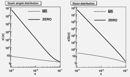
Figure 1: Comparison of the ZERO and $\overline{\rm MS}$ singlet parton distributions at $M=50\,\,{\rm GeV}$. The $\overline{\rm MS}$ distributions were obtained by evolving the starting distributions of the MRST98 set [1] with the fixed number of active flavours $n_{\rm f}=3$ (only light flavours are taken into account). The ZERO distributions were calculated numerically from the $\overline{\rm MS}$ ones. Note that the gluon distributions are plotted in their absolute value because the ZERO gluon distribution is negative in the displayed region. The point where the ZERO gluon distribution changes the sign is close to $x=0.1$.

3 The condition of applicability

A given factorization scheme obviously has no restrictions on its practical applicability if the corresponding coefficient functions, cross-sections at parton level and parton distribution functions behave for low $x$ in a similar way as the $\overline{\rm MS}$ ones. If we consider only such factorization schemes for which the corresponding matrix $\mathbf{P}^{(1)}(x)$ has the same structure as the $\overline{\rm MS}$ one, that is

$$\begin{array}[]{rccclrcccl}P^{(1)}_{q_{i}q_{j}}(x)&=&P^{(1)}_{\bar{q}_{i}\bar{q}_{j}}(x)&=&\delta_{ij}P^{(1)V}_{qq}\!(x)+P^{(1)S}_{qq}(x),&P^{(1)}_{q_{i}G}(x)&=&P^{(1)}_{\bar{q}_{i}G}(x)&=&P^{(1)}_{qG}(x),\\[8.5359pt] P^{(1)}_{q_{i}\bar{q}_{j}}(x)&=&P^{(1)}_{\bar{q}_{i}q_{j}}(x)&=&\delta_{ij}P^{(1)V}_{q\bar{q}}\!(x)+P^{(1)S}_{qq}(x),&P^{(1)}_{Gq_{i}}(x)&=&P^{(1)}_{G\bar{q}_{i}}(x)&=&P^{(1)}_{Gq}(x),\end{array}$$ (9)

then a detailed analysis of the solution of the equation (6) shows that the preceding condition of applicability is fulfilled if and only if the Mellin moments of the corresponding NLO splitting functions $P^{(1)V}_{qq}\!(n)$, $P^{(1)V}_{q\bar{q}}\!(n)$, $P^{(1)S}_{qq}(n)$, $P^{(1)}_{qG}(n)$, $P^{(1)}_{Gq}(n)$ and $P^{(1)}_{GG}(n)$ satisfy the equation

$$\,\,\,\,\,\,\,\,P^{(0)}_{Gq}(n)\left(P^{(0)}_{qq}(n)-P^{(0)}_{GG}(n)-b\right)\left(P^{(1)}_{qG}(n)-P^{(1)}_{qG}(n,\overline{\rm MS})\right)+$$

$$+\,P^{(0)}_{qG}(n)\left(P^{(0)}_{qq}(n)-P^{(0)}_{GG}(n)+b\right)\left(P^{(1)}_{Gq}(n)-P^{(1)}_{Gq}(n,\overline{\rm MS})\right)-$$

$$-\,2P^{(0)}_{qG}(n)P^{(0)}_{Gq}(n)\left(P^{(1)V}_{qq}\!(n)+P^{(1)V}_{q\bar{q}}\!(n)+2n_{\rm f}P^{(1)S}_{qq}(n)-P^{(1)}_{GG}(n)\,-\right.$$

$$\left.-\,P^{(1)V}_{qq}\!(n,\overline{\rm MS})-P^{(1)V}_{q\bar{q}}\!(n,\overline{\rm MS})-2n_{\rm f}P^{(1)S}_{qq}(n,\overline{\rm MS})+P^{(1)}_{GG}(n,\overline{\rm MS})\right)=0$$ (10)

for $n\in{\cal N}$ where

$${\cal N}_{n_{\rm f}=3}\,=\,\left\{1.7329,4.6306\right\},\quad{\cal N}_{n_{\rm f}=4}\,=\,\left\{1.7995,3.8458\right\},\quad{\cal N}_{n_{\rm f}=5}\,=\,\left\{1.9001,3.1798\right\}.$$ (11)

4 Summary and conclusion

It has been shown that not all NLO splitting functions that appear at first sight as reasonable specify practically applicable factorization schemes. The practical applicability of a factorization scheme is assured if the corresponding NLO splitting functions satisfy some nontrivial condition, which can be easily formulated in the space of Mellin moments. This condition is unfortunately not satisfied in the ZERO factorization scheme, which would otherwise be optimal for NLO Monte Carlo event generators. Hence, searching for a suitable factorization scheme which is close to the ZERO factorization scheme and satisfies the condition of applicability has already been started.

References

• [1] A.D. Martin, R.G. Roberts, W.J. Stirling and R.S. Thorne, Parton distributions: a new global analysis, Eur. Phys. J. C4 (1998) 463 [hep-ph/9803445].