Aging to Equilibrium Dynamics of SiO₂

Abstract

Molecular dynamics computer simulations are used to study the aging dynamics of SiO₂ (modeled by the BKS model). Starting from fully equilibrated configurations at high temperatures $T_{\rm i}\in\{5000$ K$,3760$ K}, the system is quenched to lower temperatures $T_{\rm f}\in\{2500$ K, 2750 K, 3000 K, 3250 K$\}$ and observed after a waiting time $t_{\rm w}$. Since the simulation runs are long enough to reach equilibrium at $T_{\rm f}$, we are able to study the transition from out-of-equilibrium to equilibrium dynamics. We present results for the partial structure factors, for the generalized incoherent intermediate scattering function $C_{q}(t_{\rm w},t_{\rm w}+t)$, and for the mean square displacement $\Delta r^{2}(t_{\rm w},t_{\rm w}+t)$. We conclude that there are three different $t_{\rm w}$ regions: (I) At very short waiting times, $C_{q}(t_{\rm w},t_{\rm w}+t)$ decays very fast without forming a plateau. Similarly $\Delta r^{2}(t_{\rm w},t_{\rm w}+t)$ increases without forming a plateau. (II) With increasing $t_{\rm w}$ a plateau develops in $C_{q}(t_{\rm w},t_{\rm w}+t)$ and $\Delta r^{2}(t_{\rm w},t_{\rm w}+t)$. For intermediate waiting times the plateau height is independent of $t_{\rm w}$ and $T_{\rm i}$. Time superposition applies, i.e. $C_{q}=C_{q}(t/t_{\rm r}^{\rm Cq})$ where $t_{\rm r}^{\rm Cq}=t_{\rm r}^{\rm Cq}(t_{\rm w})$ is a waiting time dependent decay time. Furthermore $C_{q}=C(q,t_{\rm w},t_{\rm w}+t)$ scales as $C_{q}=C(q,z(t_{\rm w},t)$ where $z$ is a function of $t_{\rm w}$ and $t$ only, i.e. independent of $q$. (III) At large $t_{\rm w}$ the system reaches equilibrium, i.e. $C_{q}(t_{\rm w},t_{\rm w}+t)$ and $\Delta r^{2}(t_{\rm w},t_{\rm w}+t)$ are independent of $t_{\rm w}$ and $T_{\rm i}$. For $C_{q}(t_{\rm w},t_{\rm w}+t)$ we find that the time superposition of intermediate waiting times (II) includes the equilibrium curve (III).

I Introduction

When a glass-forming liquid is quenched from an equilibrium state at a high temperature $T_{\rm i}$ to a non-equilibrium state at a lower temperature $T_{\rm f}$, “aging processes” set in. Provided that crystallization plays no role at $T_{\rm f}$ (e.g. due to very low crystal nucleation rates), the transition to a final (metastable) equilibrium state occurs on a time scale that corresponds to the typical equilibrium relaxation time $\tau_{\rm eq}$ of the (supercooled) liquid at $T_{\rm f}$. The dynamics of the system depends on the waiting time $t_{\rm w}$ which is the time elapsed after the temperature quench. If $\tau_{\rm eq}$ exceeds the waiting time $t_{\rm w}$ then the system is observed in a transient non-equilibrium state which corresponds to a glass for $t_{\rm w}\ll\tau_{\rm eq}$. During the aging process, i.e. for $t_{\rm w}<\tau_{\rm eq}$, thermodynamic properties such as volume and energy are changing and time translation invariance does not hold: correlation functions at time $t_{\rm w}+t$ and the time origin at $t_{\rm w}$ do depend not only on the time difference $t$ but also on the waiting time $t_{\rm w}$.

Recently this aging process has been investigated extensively with experiments Cipelletti and Ramos (2005); Lynch et al. (2008); Cianci et al. (2006); Courtland and Weeks (2003); Pham et al. (2004); Latka et al. (2009), theoretically Cugliandolo and Kurchan (1993); Bouchaud et al. (1996, 1997) and with computer simulations. For a more complete summary of previous results we refer the reader to the references Barrat et al. (2003); Binder and Kob (2005) and references therein. Computer simulation studies most similar to the work presented here are on attractive colloidal systems Foffi et al. (2004, 2005a, 2005b); Puertas et al. (2007), on the Kob-Andersen Lennard-Jones (KALJ) mixture Kob and Barrat (1997, 2000); Barrat and Kob (1999); Kob et al. (2000); Sciortino and Tartaglia (2001); Saika-Voivod and Sciortino (2004); Parsaeian and Castillo (2008, 2009); Mossa et al. (2002); Berthier (2007), and silica (SiO₂) Wahlen and Rieger (2000); Scala et al. (2003); Berthier (2007); Parsaeian et al. . In the case of silica the interpretation of the results is less clear than for the KALJ mixture; e.g. different findings Scala et al. (2003); Berthier (2007) have been reported on the violation of the fluctuation-dissipation regime during aging Cugliandolo and Kurchan (1993); Bouchaud et al. (1996, 1997). Thus, it remains open whether silica, as the prototype of a glass-forming system forming a tetrahedral network structure, exhibits a different aging dynamics than, e.g. the KALJ model, where the structure is similar to that of a closed-packed hard-sphere structure.

Recent simulation studies on amorphous silica Vollmayr et al. (1996); Wahlen and Rieger (2000); Horbach and Kob (1999); Parsaeian et al. ; Horbach et al. (1996); Berthier (2007); Vink and Barkema (2003); Saika-Voivod et al. (2001, 2004); Scala et al. (2003); Saksaengwijit et al. (2004); Reinisch and Heuer (2005); Saksaengwijit and Heuer (2006, 2007); Scheidler et al. (2001) have widely used the BKS potential van Beest et al. (1990) to model the interactions between the atoms. Although it is a simple pair potential, it reproduces various static and dynamic properties of amorphous silica very well. For BKS silica, the self-diffusion constants $D_{\alpha}$ ($\alpha={\rm Si,O}$) show two different temperature regimes: At high temperatures, $D_{\alpha}$ decays according to a power law, as predicted by the mode coupling theory (MCT) of the glass transition (note, however, that also other interpretations have been assigned to this high temperature regime). At low temperature, $D_{\alpha}$ as well as the shear viscosity $\eta$ exhibit an Arrhenius behavior with an activation energy of the order of 5 eV, in agreement with experiment (see Horbach and Kob (1999) and references therein). The temperature at which the crossover between both regimes occurs is at $T_{c}\approx 3300$ K, corresponding to the critical MCT temperature of BKS silica. Previous studies of the aging dynamics of BKS silica Wahlen and Rieger (2000); Scala et al. (2003); Berthier (2007) were performed in two steps. First, the system was fully equilibrated at a temperature $T_{\rm i}>T_{c}$. Then, the system was quenched to a low temperature $T_{\rm f}<T_{c}$, followed by the production runs. Wahlen and Rieger Wahlen and Rieger (2000) analyze time-dependent correlation functions at different waiting times $t_{\rm w}$ and Berthier Berthier (2007) and Scala et al. Scala et al. (2003) study the generalized fluctuation dissipation relation and the energy landscape Scala et al. (2003). All three studies Wahlen and Rieger (2000); Scala et al. (2003); Berthier (2007) investigate the early stages of the aging dynamics, i.e. the dynamics was explored on time scales that were much smaller than the equilibrium relaxation time $\tau_{\rm eq}$ at the temperature $T_{\rm f}$.

In this work, we also consider quenches in BKS silica from a high temperature $T_{\rm i}$ to a low temperature $T_{\rm f}$. Different from previous simulation studies, we aim at elucidating the full transient dynamics at $T_{\rm f}$ from the initial state at $t_{\rm w}=0$ to equilibrium. To this end, temperatures $T_{\rm f}$ are chosen such that the system can be fully equilibrated on the typical time span of the MD simulation. Note that the considered temperatures $T_{\rm f}\in\{2500$ K, 2750 K, 3000 K, 3250 K$\}$ are below the critical MCT temperatures $T_{\rm c}$. Thus, we have access to the full aging dynamics in the experimentally relevant Arrhenius temperature regime that we have mentioned above.

The analysis of time-dependent density correlation functions $C_{q}(t_{\rm w},t_{\rm w}+t)$ (with $q$ the wavenumber) and the mean square displacement $\Delta r^{2}(t_{\rm w},t_{\rm w}+t)$ reveal three different regimes of waiting times $t_{\rm w}$: In the case of $C_{q}(t_{\rm w},t_{\rm w}+t)$ (and similarly for $\Delta r^{2}(t_{\rm w},t_{\rm w}+t)$) at early $t_{\rm w}$, a rapid decay to zero is seen, without forming a plateau at intermediate times. Then, for larger values of $t_{\rm w}$ a plateau is formed. The height of this plateau grows with waiting time and becomes more pronounced, before in the final regime the plateau height is independent of $t_{\rm w}$ and $T_{\rm i}$. In the latter regime, time superposition holds, i.e. by scaling time with a decay time $t_{\rm r}^{\rm Cq}$ the $C_{q}$ for the different values of $t_{\rm w}$ fall onto a master curve at a given wavenumber $q$. This behavior is very similar to that found for the KALJ mixture. However, it is different from the behavior predicted by mean-field spin glass models and the activated dynamics scaling, as proposed by Wahlen and Rieger. Thus, these results suggest that the aging dynamics in silica, the prototype of a glass-former with a tetrahedral network structure, is very similar to that of simple glass-formers with a closed-packed hard-sphere-like structure. We find a difference between the KALJ mixture and SiO₂, however, in the parametric plot of $C_{q}^{\prime}(C_{q})$. For SiO₂ $C_{q}^{\prime}(C_{q})$ shows a data collapse for different sufficiently large $t_{\rm w}$ and thus $C_{q}=C(q,z(t_{\rm w},t))$ whereas this data collapse does not hold as well in the case of the KALJ mixture.

The rest of the paper is organized as follows: In the next Sec. we give the details of the BKS potential and the simulation. Then, we present the results in Sec. III, before we summarize in Sec. IV. Appendix A describes the implementation of the Nosé-Hoover thermostat used in our simulation.

II Model and Details of The Simulation

The interactions between the particles are modeled by the BKS potential van Beest et al. (1990) which has been used frequently and has proven to be reliable for the study of the dynamics of amorphous silica Vollmayr et al. (1996); Wahlen and Rieger (2000); Horbach and Kob (1999); Parsaeian et al. ; Horbach et al. (1996); Berthier (2007); Vink and Barkema (2003); Saika-Voivod et al. (2001, 2004); Scala et al. (2003); Saksaengwijit et al. (2004); Reinisch and Heuer (2005); Saksaengwijit and Heuer (2006, 2007); Scheidler et al. (2001) The functional form of the BKS potential is given by a sum of a Coulomb term, an exponential and a van der Waals term. Thus the potential between particles $i$ and $j$, a distance $r_{ij}$ apart, is given by

$$\phi(r_{ij})=\frac{q_{i}q_{j}e^{2}}{r_{ij}}+A_{ij}e^{-B_{ij}r_{ij}}-\frac{C_{ij}}{r_{ij}^{6}}\quad,$$ (1)

where $e$ is the charge of an electron and the constants $A_{ij}$, $B_{ij}$ and $C_{ij}$ are $A_{\mbox{\footnotesize SiSi}}=0.0$ eV, $A_{\mbox{\footnotesize SiO}}=18003.7572$ eV, $A_{\mbox{\footnotesize OO}}=1388.7730$ eV, $B_{\mbox{\footnotesize SiSi}}=0.0$ Å^-1, $B_{\mbox{\footnotesize SiO}}=4.87318$ Å^-1, $B_{\mbox{\footnotesize OO}}=2.76000$ Å^-1, $C_{\mbox{\footnotesize SiSi}}=0.0$ eVÅ^-6, $C_{\mbox{\footnotesize SiO}}=133.5381$ eVÅ^-6 and $C_{\mbox{\footnotesize OO}}=175.0000$ eVÅ^-6 van Beest et al. (1990). The partial charges $q_{i}$ are $q_{\mbox{\footnotesize Si}}=2.4$ and $q_{\mbox{\footnotesize O}}=-1.2$ and $e^{2}$ is given by $1602.19/(4\pi 8.8542)$ eVÅ.

The Coulombic part of the interaction was computed by using the Ewald method Kieffer and Angell (1989); Allen and Tildesley (1990) with a constant $\alpha L=6.3452$, where $L$ is the size of the cubic box, and by using all $q$-vectors with $|q|\leq 6\cdot 2\pi/L$. . We ensure that the Ewald term in real space is also differentiable at the cutoff by smoothing similarly to Eq. (3) in Pfleiderer et al. (2006) with $r_{\rm c}=8$ Å and $d=0.05$ Ų. To increase computation speed the non-Coulombic contribution to the potential was truncated, smoothed and shifted at a distance of 5.5 Å. Note that this truncation is not negligible since it affects the pressure of the system. In Ref. Pfleiderer et al. (2006) further slight variations on the potential are described in detail . In order to minimize surface effects periodic boundary conditions were used. The masses of the Si and O atoms were 28.086 u and 15.9994 u, respectively. The number of particles was 336, of which 112 were silica atoms and 224 were oxygen atoms. For all simulation runs the size of the cubic box was fixed to $L=16.920468$ Å which corresponds to a density of $\rho=2.323$ g/cm³, a value that is very close to the one of real silica glass, $\rho=2.2$ g/cm³ Brückner (1970).

Figure 1: Schematic sketch of the protocol for the simulation runs. 20 independent initial configurations are obtained via one long simulation run at $6000$ K. For each independent configuration the system is quenched instantaneously and then fully equilibrated at temperatures $T_{\rm i}=3760$ K and 5000 K, followed by instantaneous quenches to the temperatures $T_{\rm f}=3250$ K, $3000$ K, $2750$ K, and $2500$ K. At each $T_{\rm f}$, time-dependent correlation functions are determined for different waiting times $t_{\rm w}$. Temperature is kept constant at $T_{\rm f}$ by coupling the system to a Nosé-Hoover thermostat. The thermostat is switched off after 0.33 ns, followed by the continuation of the simulations in the microcanonical ensemble for $33$ ns.

We investigated the aging dynamics for systems which were quenched from a high temperature $T_{\rm i}$ to a low temperature $T_{\rm f}$. To increase the statistics, for each $(T_{\rm i},T_{\rm f})$ 20 independent simulation runs were performed. To obtain 20 independent configurations we carried out molecular dynamics (MD) simulations using the velocity Verlet algorithm with a time step of $1.6$ fs at 6000 K. The temperature was kept constant at $6000$ K with a stochastic heat bath by replacing the velocities of all particles by new velocities drawn from the corresponding Boltzmann distribution every 150 time steps. Independent configurations were at least $3.27$ ns apart. Each of these configurations undergoes the following sequence of simulation runs (see also Fig. 1). After fully equilibrating the samples at the initial temperatures $T_{\rm i}=5000$ K (for $16.35$ ns) and $T_{\rm i}=3760$ K (for $32.7$ ns), the system was quenched instantaneously to $T_{\rm f}\in\{2500\,{\rm K},2750\,{\rm K},3000\,{\rm K},3250\,{\rm K}\}$. To disturb the dynamics minimally, we used a Nosé-Hoover thermostat Hoover (1985); Brańka and Wojciechowski (2000) instead of a stochastic heat bath to keep the temperature at $T_{\rm f}$ constant. A velocity Verlet algorithm was used to integrate the Nosé-Hoover equations of motion (see Appendix A) with a time step of 1.02 fs. After $0.33$ ns the Nosé-Hoover thermostat was switched off and the simulation was continued in the NVE ensemble for $33$ ns using a time step of $1.6$ fs. Whereas previous simulations used instead the NVT ensemble for the whole simulation run, we chose to switch to the NVE ensemble to minimize any influence on the dynamics due to the chosen heat bath algorithm. For the comparison with previous simulations and to check for the lack of a temperature drift, we show in Fig. 2 for exemplatory simulation runs the temperature $T=\frac{2{\overline{E}}_{\rm kin}}{3N}$ as a function of time where ${\overline{E}}_{\rm kin}$ is the time averaged kinetic energy with fluctuations as indicated with error bars. We find that even after switching off the heat bath there is no temperature drift for $T=3250\,{\rm K}$ and $T=3000\,{\rm K}$ and for $T=2500\,{\rm K}$ and $T=2750\,{\rm K}$ there is only a slight temperature drift which is of the same order as the temperature fluctuations and the drift occurs only for $t\lessapprox 0.6$ ns. For all times $t\gtrapprox 0.6$ ns and for all investigated temperatures there is no temperature drift and thus the comparison with previous simulations valid.

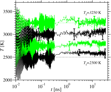
Figure 2: (Color online) Temperature $T=\frac{2{\overline{E}}_{\rm kin}}{3N}$ as a function of time $t$ for $T_{\rm i}=5000\,{\rm K}$, $T_{\rm f}=2500\,{\rm K},2750\,{\rm K},3000\,{\rm K},3250\,{\rm K}$ shown in each case for the 11th independent simulation run. ${\overline{E}}_{\rm kin}$ includes a time average and error bars indicate the corresponding fluctuations.

III Results

In all following, we investigate how the structure and dynamics of the system depend on the waiting time $t_{\rm w}$ elapsed after the quench from $T_{\rm i}$ to $T_{\rm f}$. We varied the waiting time in the range $0$ ns $\leq t_{\rm w}\leq 23.98$ ns.

III.1 Partial Structure Factor

Figure 3 shows for the temperature quench $T_{\rm i}=5000$ K to $T_{\rm f}=2500$ K the partial structure factors Binder and Kob (2005)

$$S_{\alpha\beta}(q,t_{\rm w})=\frac{1}{N}\left\langle\sum\limits_{i=1}^{N_{\alpha}}\sum\limits_{j=1}^{N_{\beta}}{\rm e}^{i{\bf q}\cdot\big{(}{\bf r}_{i}(t_{\rm w})-{\bf r}_{j}(t_{\rm w})\big{)}}\right\rangle$$ (2)

where ${\bf r}_{i}$ and ${\bf r}_{j}$ are the positions of particles $i$ and $j$ of species $\alpha,\beta={\rm O,Si}$. The partial structure factors for all other $(T_{\rm i},T_{\rm f})$ combinations are very similar. Although Fig. 3 shows $S(q,t_{\rm w})$ for the largest investigated temperature quench, there is only a slight $t_{\rm w}$-dependence for very short waiting times $t_{\rm w}\leq 0.33$ ns and almost no $t_{\rm w}$-dependence for $t_{\rm w}\geq 0.33$ ns.

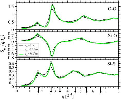
Figure 3: (Color online) Partial structure factors $S_{\alpha\beta}(q,t_{\rm w})$ as defined in Eq. (2) for the temperature quench $T_{\rm i}=5000$ K to $T_{\rm f}=2500$ K. Indicated with arrows are the wave vectors $q$ which have been used to determine $C_{q}(t_{\rm w},t_{\rm w}+t)$ as defined in Eq. (3).

III.2 Generalized Incoherent Intermediate Scattering Function

In this section we focus on the time-dependent generalized intermediate incoherent scattering function Binder and Kob (2005)

$$C_{q}(t_{\rm w},t_{\rm w}+t)=\frac{1}{N_{\alpha}}\left\langle\sum\limits_{j=1}^{N_{\alpha}}{\rm e}^{i{\bf q}\cdot\big{(}{\bf r}_{j}(t_{\rm w}+t)-{\bf r}_{j}(t_{\rm w})\big{)}}\right\rangle$$ (3)

which is a measure for the correlations of the positions at time $t_{\rm w}$ and at a later time $(t_{\rm w}+t)$. We investigated wave vectors of magnitude $q=1.7,2.7,3.4,4.6,5.5$ and $6.6$ Å^-1, as indicated with arrows in Fig. 3. We show in Fig. 4 and Figs. 6 - 8 results for the first sharp diffraction peak at $q=1.7$ Å^-1. Similar results are found for all other investigated wave vectors. Figure 4 shows $C_{q}(t_{\rm w},t_{\rm w}+t)$ for the largest investigated temperature quench from $T_{\rm i}=5000$ K to $T_{\rm f}=2500$ K for waiting times $t_{\rm w}=0$ - 23.98 ns, as listed in the figure caption of Fig. 4. We find that $C_{q}(t_{\rm w},t_{\rm w}+t)$ is dependent on $t_{\rm w}$ for all but the last three investigated waiting times. For very short times $t\lesssim 5\cdot 10^{-5}$ ns and zero waiting time, $C_{q}(t_{\rm w}=0,t)$ is well approximated by $C_{q}$ of the high temperature $T_{\rm i}=5000$ K from which the system has been quenched (see dashed line in Fig. 4). Thus, $C_{q}(t_{\rm w}=0,t)$ for very short times is only dependent on $T_{\rm i}$, $q$ and the particle type, but independent of $T_{\rm f}$. For times of the order of $t=10^{-3}$ ns, $C_{q}(t_{\rm w},t_{\rm w}+t)$ is oscillatory due to the small system size. For times $t\gtrsim 10^{-3}$ ns, $C_{q}$ decays to zero without forming a plateau for small $t_{\rm w}$. With increasing $t_{\rm w}$ a plateau is formed, which is independent of $t_{w}$ for $t_{\rm w}\geq 0.33$ ns.

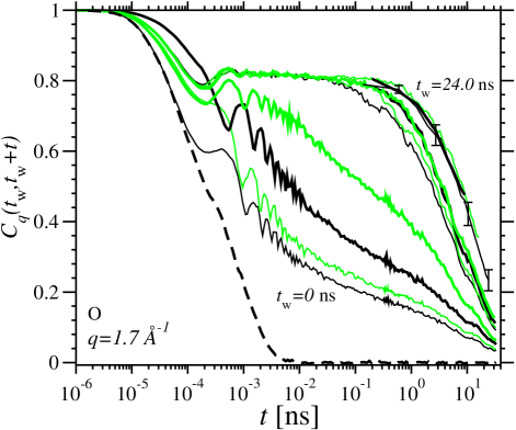
Figure 4: (Color online) $C_{q}(t_{\rm w},t_{\rm w}+t)$ as defined in Eq. (3) for the quench $T_{\rm i}=5000$ K to $T_{\rm f}=2500$ K for O-atoms and $q=1.7$ Å^-1. Waiting times for the solid lines are from bottom to top $t_{\rm w}=0$ ns, $1.63\cdot 10^{-4}$ ns, $1.63\cdot 10^{-3}$ ns, $1.63\cdot 10^{-2}$ ns, $0.33$ ns, $0.49$ ns, $1.17$ ns, $1.96$ ns, $8.83$ ns, $16.67$ ns, and $23.98$ ns. The order of solid lines are for increasing $t_{\rm w}$ black thin, green (gray) thin, black thick, green (gray) thick, black thin, green (gray) thin, etc. Error bars are as indicated exemplary. The thick dashed line corresponds to $C_{q}(t_{\rm w},t_{\rm w}+t)=F_{\rm s}(q,t)$ at $5000$ K.

To characterize the plateau height we define $F$ as the time average of $C_{q}(t_{\rm w},t_{\rm w}+t)$ for times $2.55$ ps $\leq t\leq 6.64$ ps. The inset of Fig. 5 shows that for large waiting times $F(t_{\rm w})$ becomes independent of $t_{\rm w}$ and of $T_{\rm i}$. To test this independence of $T_{\rm i}$ further, we show $F$ as a function of $q$ for $t_{\rm w}=16.67$ ns in Fig. 5. We find that the plateau height is dependent on the particle type and decreases with decreasing $q$, but $F$ is independent of $T_{\rm i}$.

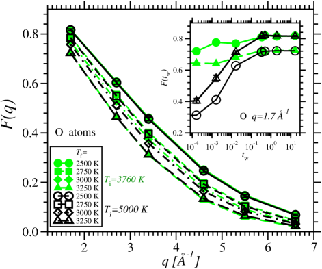
Figure 5: (Color online) Plateau height, $F$, as defined in the text, as a function of wave vector $q$ ($t_{\rm w}=16.67$ ns) and in the inset as a function of $t_{\rm w}$ ($q=1.7$ Å^-1). Error bars are of the same size as symbols as indicated exemplary for $T_{\rm i}=5000$ K and $T_{\rm f}=2500$ K.

The plateau in $C_{q}$ becomes more horizontal with decreasing final temperature $T_{\rm f}$, as can be seen by the comparison of Fig. 4 ($T_{\rm f}=2500$ K) and Fig. 6 ($T_{\rm f}=3000$ K). Times $t\gtrsim 0.1$ ns correspond to the $\alpha$-relaxation, where $C_{q}(t_{\rm w},t_{\rm w}+t)$ decays from the plateau to zero. For the quench from $5000$ K to $2500$ K (see Fig. 4) this decay depends on $t_{\rm w}$ for all $t_{\rm w}<8.83$ ns. However, for $t_{\rm w}\geq 8.83$ ns (the largest three $t_{\rm w}$), $C_{q}(t_{\rm w},t_{\rm w}+t)$ is independent of $t_{\rm w}$ not only for intermediate times $t$ (plateau) but for all times (including the $\alpha$-relaxation). Thus, the system reaches equilibrium during the simulation run. For the quench from $3760$ K to $3000$ K (see Fig. 6), $C_{q}(t_{\rm w},t_{\rm w}+t)$ becomes independent of $t_{\rm w}$ for $t_{\rm w}\gtrsim 1$ ns, which means that the time at which equilibrium is reached is dependent on the temperature quench.

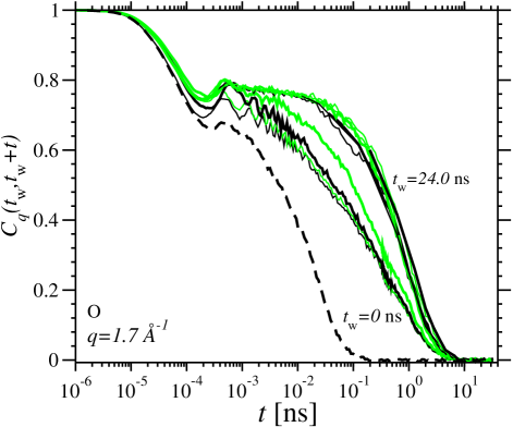
Figure 6: (Color online) $C_{q}(t_{\rm w},t_{\rm w}+t)$ for the quench $T_{\rm i}=3760$ K to $T_{\rm f}=3000$ K. Waiting times and corresponding line styles are the same as in Fig. 4. Error bars are of the same order as indicated in Fig. 4. The thick dashed line corresponds to $C_{q}(t_{\rm w},t_{\rm w}+t)=F_{\rm s}(q,t)$ at $3760$ K.

To estimate the time when the system reaches equilibrium for each $(T_{\rm i},T_{\rm f})$ combination, we next quantify the decay of $C_{q}(t_{\rm w},t_{\rm w}+t)$ . Instead of taking a vertical cut in $C_{q}(t_{\rm w},t_{\rm w}+t)$ as we did for $F$, we now take a horizontal cut. We define the decay time $t_{\rm r}^{\rm Cq}$ to be the time $t=t_{\rm r}^{\rm Cq}$ for which $C_{q}(t_{\rm w},t_{\rm w}+t_{\rm r}^{\rm Cq})=C_{\rm cut}$. We chose $C_{\rm cut}=0.625/0.41/0.295/0.155/0.085/0.04)$ for the Si particles and $C_{\rm cut}=0.625/0.305/0.195/0.08/0.04/0.014$ for the O particles at the wavenumbers $q=1.7/2.7/3.4/4.6/5.5/6.6$ Å^-1, respectively. The resulting decay times $t_{\rm r}^{\rm Cq}$ as a function of waiting time $t_{\rm w}$ are shown in Fig. 7a for O-atoms and in Fig. 7b for Si-atoms. Color (black or green/gray) indicates the initial temperature $T_{\rm i}$ and symbol shape indicates the final temperature $T_{\rm f}$.

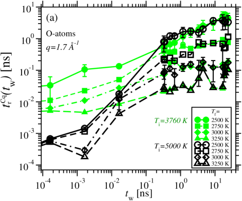
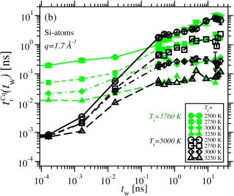
Figure 7: (Color online) Decay time $t_{\rm r}^{\rm Cq}$ for $q=1.7$ Å^-1 and (a) O-atoms and (b) Si-atoms. Green (gray) is used for $T_{\rm i}=3760$ K and black for $T_{\rm i}=5000$ K. Symbol shape indicates $T_{\rm f}$ as given in the legend. Error bars are given exemplary for ($T_{\rm i}=3760$ K, $T_{\rm f}=2500$ K), ($T_{\rm i}=5000$ K, $T_{\rm f}=2500$ K) and ($T_{\rm i}=5000$ K, $T_{\rm f}=3000$ K).

We find that $t_{\rm r}^{\rm Cq}(t_{\rm w})$ is characterized by three different $t_{\rm w}$-windows. (I) For waiting times $t_{\rm w}\lesssim 0.3$ ns, decay times are significantly lower for $T_{\rm i}=5000$ K (black lines and symbols) than for $T_{\rm i}=3760$ K (green/gray lines and symbols). The dependence of $t_{\rm r}^{\rm Cq}$ on $t_{\rm w}$ is strongly dependent on all varied parameters, i.e. $T_{\rm i}$, $T_{\rm f}$, particle type, and $q$. For $T_{\rm i}=5000$ K, $T_{\rm f}=2500$ K, $2750$  K, and $q=1.7$ Å^-1, $2.7$ Å^-1 $t_{\rm r}^{\rm Cq}(t_{\rm w})$ follows roughly a power law with an exponent $\mu\approx 1.15$ with variations of the order of $0.07$ dependent on $T_{\rm f}$, particle type, and $q$. (II) For intermediate waiting times, $t_{\rm r}^{\rm Cq}(t_{\rm w})$ also follows roughly a power law with a different exponent than in regime (I). We find for $T_{\rm i}=5000$ K, $T_{\rm f}=2500$ K, $2750$ K and $q=1.7$ Å^-1, $2.7$ Å^-1 $\mu\approx 0.35$ with variations of the order of $0.08$ depending on $T_{\rm f}$, particle type, and $q$. Best power law fits are for $T_{\rm i}=3760$ K, $T_{\rm f}=2500$ K with $\mu$ ranging from $\mu=0.55$/$0.57$ for $q=1.7$ Å^-1 to $\mu=0.69$/$0.63$ for $q=6.6$ Å^-1 and for Si/O atoms. Kob and Barrat find for the binary Lennard-Jones system also a power law for $t_{\rm r}^{\rm Cq}(t_{\rm w})$, however, with $\mu=0.882$ Kob and Barrat (1997). Similar to Grigera et al. Grigera et al. (2004) we find that the transition from small waiting times (I) to intermediate waiting times (II) is accompanied by a change of the exponent $\mu$. (III) For very long waiting times $t_{\rm r}^{\rm Cq}(t_{\rm w})$ is independent of $t_{\rm w}$ and $T_{\rm i}$, i.e. equilibrium is reached. The waiting time $t_{23}$ for which the transition from regime (II) to regime (III) occurs is dependent on $T_{\rm f}$: $t_{23}\approx 0.3$ ns for $T_{\rm f}=3250$ K, $t_{23}\approx 1$ ns for $T_{\rm f}=3000$ K, $t_{23}\approx 3$ ns for $T_{\rm f}=2750$ K, and $t_{23}\approx 10$ ns for $T_{\rm f}=2500$ K.

Mean-field spin glass models predict Bouchaud et al. (1996, 1997)

$$C_{q}(t_{\rm w},t_{\rm w}+t)=C_{q}^{\rm ST}(t)+C_{q}^{\rm AG}\left(\frac{h(t_{\rm w}+t)}{h(t_{\rm w})}\right)\;,$$ (4)

according to which $C_{q}(t_{\rm w},t_{\rm w}+t)$ can be separated into a short-time term $C_{q}^{\rm ST}(t)$ that is independent of $t_{w}$ and an intermediate-time term that scales as $h(t_{\rm w}+t)/h(t_{\rm w})$ where $h$ is a monotonously increasing function. It has been observed for different systems that the function $h(t)$ follows $h(t)\approx t^{\alpha}$. Thus, the so-called “simple aging” (see Kob and Barrat (1997) and references therein) applies and, as a consequence, $C_{q}$ as a function of $(t/t_{\rm w})$ for different $t_{\rm w}$ superimpose.

Müssel and Rieger Müssel and Rieger (1998) have proposed activated dynamics for $C_{q}(t_{\rm w},t_{\rm w}+t)$,

$$C_{q}(t_{\rm w},t_{\rm w}+t)=C_{q}^{\rm ST}(t)+C_{q}^{\rm AG}\left(\frac{{\rm ln}\left[(t_{\rm w}+t)/\tau_{\rm fit}\right]}{{\rm ln}\left[t_{\rm w}/\tau_{\rm fit}\right]}\right),$$ (5)

where the characteristic time scale $\tau_{\rm fit}$ is a fit parameter. We find that neither $C_{q}\left(\frac{t_{\rm w}+t}{t_{\rm w}}\right)$, nor $C_{q}\left(\frac{t}{t_{\rm w}}\right)$, nor $C_{q}\left(\frac{{\rm ln}\left[(t_{\rm w}+t)/\tau_{\rm fit}\right]}{{\rm ln}\left[t_{\rm w}/\tau_{\rm fit}\right]}\right)$ (for any choice of $\tau_{\rm fit}$) superimpose for different $t_{\rm w}$. Instead we find, similar to the results of Kob and Barrat Kob and Barrat (1997) for a binary Lennard-Jones system, that time superposition holds, defined by

$$C_{q}(t_{\rm w},t_{\rm w}+t)=C_{q}^{\rm ST}(t)+C_{q}^{\rm AG}\left(\frac{t}{t_{\rm r}^{\rm Cq}(t_{\rm w})}\right)\,.$$ (6)

In Fig. 8, we show $C_{q}(t/t_{\rm r}^{\rm Cq})$ for the same set of parameters as in Fig. 4. When all waiting times are included (see inset of Fig. 8) time superposition does not apply due to including too short waiting times. Wahlen and Rieger Wahlen and Rieger (2000) have studied $C_{q}(t_{\rm w},t_{\rm w}+t)$ for the same BKS-SiO₂ system, however for waiting times smaller than $50$ ps. Their results are consistent with the inset of Fig. 8. For waiting times $t_{\rm w}\geq 0.49$ ns (see Fig. 8), however, Eq. (6) is a good approximation. Please note that $C_{q}(t/t_{\rm r}^{\rm Cq})$ follows time superposition for all waiting times $t_{\rm w}\geq 0.49$ ns, i.e. not only for the time-range (II), but also for the time-range (III). That means for the $\alpha$-relaxation that the shape of the out-of equilibrium curves is the same (within error bars) as the shape of the equilibrium curves. We find similar results for all other $(T_{\rm i},T_{\rm f})$ combinations, Si-particles, and all other $q$.

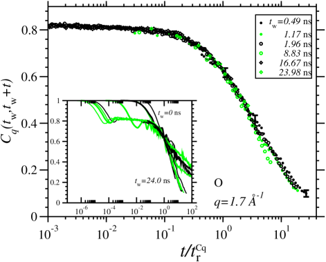
Figure 8: (Color online) $C_{q}(t/t_{\rm r}^{\rm Cq})$ for the quench from $T_{\rm i}=2500$ K to $T_{\rm i}=5000$ K for O-atoms and $q=1.7$ Å^-1. Waiting times and corresponding lines in the inset are the same as in Fig. 4.

Next we test whether $C_{q}=C(q,t_{\rm w},t_{\rm w}+t)$ scales as $C_{q}=C(q,z(t_{\rm w},t)$ where $z$ is a function of $t_{\rm w}$ and $t$ only, i.e. independent of $q$. Following an approach of Kob and Barrat Kob and Barrat (2000) we show in Figure 9 a parametric plot for $C_{q^{\prime}}(t_{\rm w},t_{\rm w}+t)$ as a function of $C_{q}(t_{\rm w},t_{\rm w}+t)$ for $q=1.7$ Å^-1 and $q^{\prime}=2.7$, 3.4, 4.6, 5.5, 6.6 Å^-1 for O-atoms and the temperature quench from $5000$ K to $2500$ K. For sufficiently large $t_{\rm w}$ we find, contrary to the results of Kob and Barrat for the Lennard-Jones system, that for SiO₂ the parametric curves superimpose and thus that $C(q,t_{\rm w},t_{\rm w}+t)=C(q,z(t_{\rm w},t)$ for $t_{\rm w}\geq 0.49$ ns. This includes, within error bars, also the equilibrated curves for $t_{\rm w}\gtrsim 10$ ns. We find similar results for all other $(T_{\rm i},T_{\rm f})$ combinations, Si-particles, and all other $q$.

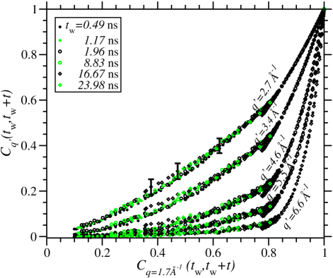
Figure 9: (Color online) $C_{q^{\prime}}(t_{\rm w},t_{\rm w}+t)$ as a function of $C_{q}(t_{\rm w},t_{\rm w}+t)$ for $q=1.7$ Å^-1 and $q^{\prime}=2.7$, 3.4, 4.6, 5.5, 6.6 Å^-1 for O-atoms and the temperature quench from $5000$ K to $2500$ K.

III.3 Mean Square Displacement

In the previous section, we have focused on the analysis of $C_{q}(t_{\rm w},t_{\rm w}+t)$ and identified different time-windows. In this section, we consider the mean square displacement

$$\Delta r^{2}(t_{\rm w},t_{\rm w}+t)\,=\,\frac{1}{N}\,\sum\limits_{i=1}^{N}\left\langle\left({\bf r}_{i}(t_{\rm w}+t)-{\bf r}_{i}(t_{\rm w})\right)^{2}\right\rangle\,.$$ (7)

Figure 10 shows $\Delta r^{2}(t_{\rm w},t_{\rm w}+t)$ for the temperature quench from $5000$ K to $2500$ K and for O-atoms. As in Fig. 4, for times $t\lesssim 5\cdot 10^{-5}$ ns and zero waiting time, the mean square displacement $\Delta r^{2}(t_{\rm w}=0,t)$ is well approximated by $\Delta r^{2}$ of the high temperature $T_{\rm i}=5000$ K from which the system has been quenched (see dashed line in Fig. 10) and thus independent of $T_{\rm f}$. For times $t\approx 10^{-3}$ ns, $\Delta r^{2}(t_{\rm w},t_{\rm w}+t)$ is oscillatory due to the small system size Horbach et al. (1996), while for times $t\gtrsim 10^{-3}$ ns and waiting times $t_{\rm w}\geq 0.33$ ns, we find that $\Delta r^{2}$ forms a plateau which is independent of $t_{w}$. As for $C_{q}$, we find that the plateau is the more horizontal the smaller $T_{\rm f}$ and the plateau height depends on the particle type but is independent of $T_{\rm i}$.

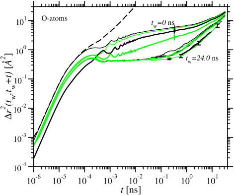
Figure 10: (Color online) Mean square displacement $\Delta r^{2}(t_{\rm w},t_{\rm w}+t)$ as defined in Eq. (7) for the temperature quench from $5000$ K to $2500$ K and for O-atoms. Waiting times and corresponding line styles are the same as in Fig. 4.

For waiting times $t_{\rm w}\geq 0.33$ ns and times $t\gtrsim 0.1$ ns, the mean square displacement leaves the plateau and increases further. To characterize the dependence of this $\alpha$-relaxation we define the time $t_{\rm r}^{\rm msd}$ as the time $t=t_{\rm r}^{\rm msd}$ for which $\Delta r^{2}(t_{\rm w},t_{\rm w}+t_{\rm r}^{\rm msd})=1.35$ Ų (see Fig. 11). We can identify again the three time windows (I) of waiting times $t_{\rm w}\lesssim 0.3$ ns with a dependence on $T_{\rm i}$, $T_{\rm f}$ and particle type, (II) the aging regime of intermediate waiting times where $t_{\rm r}^{\rm msd}$ follows roughly a power law, and (III) for very long waiting times when equilibrium is reached. The transition from (II) to (III) occurs at approximately the same times $t_{23}$ as for $C_{q}$, i.e. $t_{23}\approx 0.3$ ns for $T_{\rm f}=3250$ K, $t_{23}\approx 1$ ns for $T_{\rm f}=3000$ K, $t_{23}\approx 3$ ns for $T_{\rm f}=2750$ K and $t_{23}\approx 10$ ns for $T_{\rm f}=2500$ K.

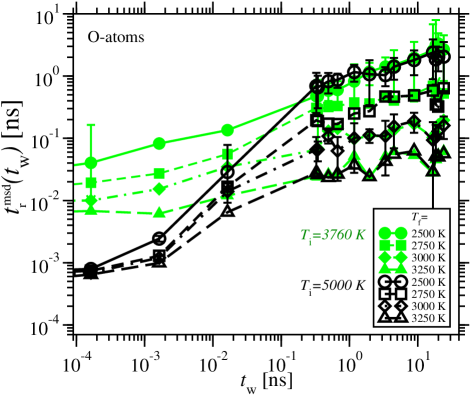
Figure 11: (Color online) $t_{\rm r}^{\rm msd}$ for O-atoms. Symbols for the different $(T_{\rm i},T_{\rm f})$ combinations are the same as in Fig. 7. Error bars are indicated exemplary for ($3760$ K, $2500$ K), ($5000$ K, $2500$ K) and ($5000$ K, $3000$ K).

Figure 12 shows the equivalent of Fig. 8 to test time superposition. We find for $\Delta r^{2}(t/t_{\rm r}^{\rm msd})$ that time superposition is valid for waiting times $0.34$ ns $\leq t_{\rm w}\lesssim 8.83$ ns, i.e. for the time window (II) but not for the time window (III).

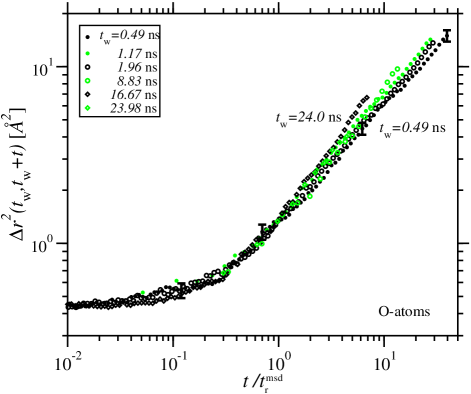
Figure 12: (Color online) $\Delta r^{2}(t/t_{\rm r}^{\rm msd})$ for the temperature quench from $5000$ K to $2500$ K and for O-atoms.

IV Summary

Using molecular dynamics simulations, we investigated for the strong glass former SiO₂ the aging dynamics below the critical MCT temperature $T_{c}$, using the BKS potential to model the interactions between silicon and oxygen atoms. After an instantaneous quench from $T_{\rm i}>T_{c}$ to a temperature $T_{\rm f}<T_{c}$ the dynamics towards equilibrium was studied as a function of waiting time $t_{\rm w}$. Note that the temperatures $T_{\rm f}$ were chosen such that equilibrium was reached on the time span of the simulations (of the order of 30 ns). The central quantities considered in this work are the incoherent intermediate scattering function $C_{q}(t_{\rm w},t_{\rm w}+t)$ and the mean square displacement $\Delta r^{2}(t_{\rm w},t_{\rm w}+t)$. These functions depend on the time origin at $t_{\rm w}$ as long as $t_{\rm w}$ is smaller than the typical relaxation time, $\tau_{\rm eq}$, that is required to equilibrate the system.

We find that the decay of $C_{q}(t_{\rm w},t_{\rm w}+t)$ (and similarly the rise of $\Delta r^{2}(t_{\rm w},t_{\rm w}+t)$) exhibit qualitative changes from short to long waiting times. At short waiting times, relaxation processes are dominant that correspond to the early $\beta$ relaxation regime at the target temperature $T_{\rm f}$. In this $t_{\rm w}$ regime, no well-defined plateau is found in $C_{q}(t_{\rm w},t_{\rm w}+t)$ (see Fig. 4). Instead, this function first decreases rapidly, followed by a strongly stretched exponential decay to zero. At long waiting times, the $\beta$ relaxation seems to be very similar to that at equilibrium. The Debye-Waller factor (i.e. the height of the plateau in $C_{q}(t_{\rm w},t_{\rm w}+t)$) has reached its equilibrium value, although the decay of $C_{q}(t_{\rm w},t_{\rm w}+t)$ from the plateau to zero is faster than that at equilibrium. However, the shape of curves describing the long-time decay of $C_{q}(t_{\rm w},t_{\rm w}+t)$ is the same as that at equilibrium. Thus, $C_{q}$ follows a simple time superposition for long waiting times, different e.g. from the “activated dynamics scaling” proposed by Wahlen and Rieger for BKS silica.

Our results show that the aging dynamics of BKS silica is very similar to that of the KALJ mixture. For both silica and the KALJ mixture three $t_{\rm w}$-regimes can be identified and $C_{q}$ follows time superposition for sufficiently large $t_{\rm w}$. The only difference between these two systems is that $C_{q}$ scales as $C(q,z(t_{\rm w},t)$ for SiO₂ but less well for the KALJ mixture. So slightly below its critical temperature $T_{\rm c}$ of MCT, the strong glass-former silica does not seem to be very different from typical fragile systems, although one has already reached the low temperature Arrhenius regime (note that activation energies for the self-diffusion, viscosity etc. are of the order of 5 eV, similar to the corresponding activation energies close to the glass transition temperature $T_{\rm g}\approx 1450$ K, as measured in various experiments). However, the dynamics could be very different at very low temperatures (close to $T_{\rm g}$) where the long-time aging regime is not accessible by computer simulations. Thus, more experimental work on the aging dynamics of silica around $T_{\rm g}$ would be very desirable. We also leave for future work to test whether also for other systems three $t_{\rm w}$-regimes are identified and whether the equilibrium curve is included in the time superposition of $C_{q}$ at intermediate and large $t_{\rm w}$.

Appendix A Velocity Verlet Nosé Hoover

The Nosé Hoover equations of motion are for particles $i=1,\ldots,N$ at position $\bf{r}_{i}$ with momentum $\bf{p}_{i}$

$$\dot{\bf r}_{i} = \frac{{\bf p}_{i}}{m_{i}}$$ (8)

$$\dot{\bf p}_{i} = {\bf F}_{i}-\zeta{\bf p}_{i}$$ (9)

$$\dot{\zeta} = \frac{1}{Q}\left(\sum\limits_{i=1}^{N}\frac{{\bf p}_{i}^{2}}{m_{i}}-XkT\right)$$ (10)

and thus

$$\ddot{\bf r}_{i} = \frac{{\bf F}_{i}}{m_{i}}-\zeta\,\dot{\bf r}_{i}$$ (11)

$$\frac{{\rm d}^{2}\ln s}{{\rm d}t^{2}}=\dot{\zeta} = \frac{1}{Q}\left(\sum\limits_{i=1}^{N}m_{i}\dot{{\bf r}}_{i}^{2}-XkT\right)$$ (12)

where $X=3N$ . We integrated with the generalized velocity Verlet form of Fox and Andersen Fox and Andersen (1984)

$${\bf r}_{i}(t+\Delta t) = {\bf r}_{i}(t)+\Delta t\,\dot{\bf r}_{i}(t)$$

$$+ \frac{(\Delta t)^{2}}{2}\left(\frac{{\bf F}_{i}(t)}{m_{i}}-\zeta(t)\,\dot{\bf r}_{i}(t)\right)$$

$$\ln s(t+\Delta t) = \ln s(t)+\Delta t\,\zeta(t)$$

$$+ \frac{(\Delta t)^{2}}{2Q}\left(\sum\limits_{i=1}^{N}m_{i}\dot{\bf{r}}_{i}^{2}(t)-XkT\right)$$

$$\zeta^{\rm approx}(t+\Delta t) = \zeta(t)$$

$$+ \frac{\Delta t}{Q}\left(\sum\limits_{i=1}^{N}m_{i}\dot{\bf{r}}_{i}^{2}(t)-XkT\right)$$

$$\dot{\bf r}_{i}(t+\Delta t) = \dot{\bf r}_{i}(t)$$

$$+ \frac{\Delta t}{2}\bigg{(}\frac{{\bf F}_{i}(t)+{\bf F}_{i}(t+\Delta t)}{m_{i}}$$

$$-\big{[}\zeta(t)+\zeta^{\rm approx}(t+\Delta t)\big{]}\dot{\bf r}_{i}(t)\bigg{)}$$

$$\bigg{(}1-\frac{\Delta t}{2}\zeta^{\rm approx}(t+\Delta t)\bigg{)}$$

$$\zeta(t+\Delta t) = \zeta(t)+\frac{\Delta t}{2Q}\Big{(}\sum\limits_{i=1}^{N}m_{i}\dot{\bf{r}}_{i}^{2}(t)$$

$$+\sum\limits_{i=1}^{N}m_{i}\dot{\bf{r}}_{i}^{2}(t+\Delta t)-2XkT\Big{)}$$

To ensure that $\Upsilon=\sum\limits_{i=1}^{N}\frac{{\bf p}_{i}^{2}}{2m_{i}}+U(\{{\bf r}_{i}\})+\frac{Q}{2}\zeta^{2}+XkT\ln s$ is conserved (see Brańka and Wojciechowski (2000)) we chose $Q=50000$ Ų u.

References

- Cipelletti and Ramos (2005) L. Cipelletti and L. Ramos, J. Phys.: Condens. Matter 17, R253 (2005).
- Lynch et al. (2008) J. M. Lynch, G. C. Cianci, and E. R. Weeks, Phys. Rev. E 78, 031410 (2008).
- Cianci et al. (2006) G. C. Cianci, R. E. Courtland, and E. R. Weeks, Solid State Commun. 139, 599 (2006).
- Courtland and Weeks (2003) R. E. Courtland and E. R. Weeks, J. Phys.: Condens. Matter 15, S359 (2003).
- Pham et al. (2004) K. N. Pham, S. U. Egelhaaf, P. N. Pusey, and W. C. K. Poon, Phys. Rev. E 69, 011503 (2004).
- Latka et al. (2009) A. Latka, Y. Han, A. M. Alsayed, A. B. Schofield, A. G. Yodh, and P. Habdas, Europhys. Lett. 86, 58001 (2009).
- Cugliandolo and Kurchan (1993) L. F. Cugliandolo and J. Kurchan, Phys. Rev. Lett. 71, 173 (1993).
- Bouchaud et al. (1996) J.-P. Bouchaud, L. F. Cugliandolo, J. Kurchan, and M. Mèzard, Physica A 226, 243 (1996).
- Bouchaud et al. (1997) J.-P. Bouchaud, L. F. Cugliandolo, M. Mèzard, and J. Kurchan, arXiv.org arXiv:cond-mat/9702070v1 [cond-mat.dis-nn] (1997).
- Barrat et al. (2003) J.-L. Barrat, M. Feigelman, J. Kurchan, and J. Dalibard, eds., Slow Relaxations and Nonequilibrium Dynamics in Condensed Matter (Springer, 2003).
- Binder and Kob (2005) K. Binder and W. Kob, Glassy Materials and Disordered Solids – An Introduction to Their Statistical Mechanics (World Scientific, London, 2005).
- Foffi et al. (2004) G. Foffi, E. Zaccarelli, S. Buldyrev, F. Sciortino, and P. Tartaglia, J. Chem. Phys. 120, 8824 (2004).
- Foffi et al. (2005a) G. Foffi, C. DeMichele, F. Sciortino, and P. Tartaglia, Phys. Rev. Lett. 94, 078301 (2005a).
- Foffi et al. (2005b) G. Foffi, C. D. Michele, F. Sciortino, and P. Tartaglia, J. Chem. Phys. 122, 224903 (2005b).
- Puertas et al. (2007) A. M. Puertas, M. Fuchs, and M. E. Cates, Phys. Rev. E 75, 031401 (2007).
- Kob and Barrat (1997) W. Kob and J.-L. Barrat, Phys. Rev. Lett. 78, 4581 (1997).
- Kob and Barrat (2000) W. Kob and J.-L. Barrat, Eur. Phys. J. B 13, 319 (2000).
- Barrat and Kob (1999) J.-L. Barrat and W. Kob, Europhys. Lett. 46, 637 (1999).
- Kob et al. (2000) W. Kob, F. Sciortino, and P. Tartaglia, Europhys. Lett. 49, 590 (2000).
- Sciortino and Tartaglia (2001) F. Sciortino and P. Tartaglia, J. Phys.: Condens. Matter 13, 9127 (2001).
- Saika-Voivod and Sciortino (2004) I. Saika-Voivod and F. Sciortino, Phys. Rev. E 70, 041202 (2004).
- Parsaeian and Castillo (2008) A. Parsaeian and H. E. Castillo, Phys. Rev. E 78, 060105(R) (2008).
- Parsaeian and Castillo (2009) A. Parsaeian and H. E. Castillo, Phys. Rev. Lett. 102, 055704 (2009).
- Mossa et al. (2002) S. Mossa, G. Ruocco, F. Sciortino, and P. Tartaglia, Philos. Mag. B 82, 695 (2002).
- Berthier (2007) L. Berthier, Phys. Rev. Lett. 98, 220601 (2007).
- Wahlen and Rieger (2000) H. Wahlen and H. Rieger, J. Phys. Soc. Japan Suppl. A 69, 242 (2000).
- Scala et al. (2003) A. Scala, C. Valeriani, F. Sciortino, and P. Tartaglia, Phys. Rev. Lett. 90, 115503 (2003).
- (28) A. Parsaeian, H. E. Castillo, and K. Vollmayr-Lee, to be published.
- Vollmayr et al. (1996) K. Vollmayr, W. Kob, and K. Binder, Phys. Rev. B 54, 15808 (1996).
- Horbach and Kob (1999) J. Horbach and W. Kob, Phys. Rev. B 60, 3169 (1999).
- Horbach et al. (1996) J. Horbach, W. Kob, K. Binder, and C. A. Angell, Phys. Rev. E 54, R5897 (1996).
- Vink and Barkema (2003) R. L. C. Vink and G. T. Barkema, Phys. Rev. B 67, 245201 (2003).
- Saika-Voivod et al. (2001) I. Saika-Voivod, P. H. Poole, and F. Sciortino, Nature 412, 514 (2001).
- Saika-Voivod et al. (2004) I. Saika-Voivod, F. Sciortino, T. Grande, and P. H. Poole, Phys. Rev. E 70, 061507 (2004).
- Saksaengwijit et al. (2004) A. Saksaengwijit, J. Reinisch, and A. Heuer, Phys. Rev. Lett. 93, 235701 (2004).
- Reinisch and Heuer (2005) J. Reinisch and A. Heuer, Phys. Rev. Lett. 95, 155502 (2005).
- Saksaengwijit and Heuer (2006) A. Saksaengwijit and A. Heuer, Phys. Rev. E 73, 061503 (2006).
- Saksaengwijit and Heuer (2007) A. Saksaengwijit and A. Heuer, J. Phys.: Condens. Matter 19, 205143 (2007).
- Scheidler et al. (2001) P. Scheidler, W. Kob, A. Latz, J. Horbach, and K. Binder, Phys. Rev. B 63, 104204 (2001).
- van Beest et al. (1990) B. W. H. van Beest, G. J. Kramer, and R. A. van Santen, Phys. Rev. Lett. 64, 1955 (1990).
- Kieffer and Angell (1989) J. Kieffer and C. A. Angell, J. Chem. Phys. 90, 4982 (1989).
- Allen and Tildesley (1990) M. P. Allen and D. J. Tildesley, Computer Simulation of Liquids (Oxford University Press, New York, 1990).
- Pfleiderer et al. (2006) P. Pfleiderer, J. Horbach, and K. Binder, Chem. Geol. 229, 186 (2006).
- Brückner (1970) R. Brückner, J. Non-Cryst. Solids 5, 123 (1970).
- Hoover (1985) W. G. Hoover, Phys. Rev. A 31, 1695 (1985).
- Brańka and Wojciechowski (2000) A. C. Brańka and K. W. Wojciechowski, Phys. Rev. E 62, 3281 (2000).
- Grigera et al. (2004) T. S. Grigera, V. Martín-Mayor, G. Parisi, and P. Verrocchio, Phys. Rev. B 70, 014202 (2004).
- Müssel and Rieger (1998) U. Müssel and H. Rieger, Phys. Rev. Lett. 81, 930 (1998).
- Fox and Andersen (1984) J. R. Fox and H. C. Andersen, J. Phys. Chem. 88, 4019 (1984).
- Abramovitz and Stegun (1972) M. Abramovitz and I. A. Stegun, Handbook of Mathematical Functions (Dover Publications, New York, 1972).