LoCuSS: A Comparison of Cluster Mass Measurements from XMM-Newton and Subaru — Testing Deviation from Hydrostatic Equilibrium and Non-Thermal Pressure Support

Abstract

We compare X-ray hydrostatic and weak-lensing mass estimates for a sample of 12 clusters that have been observed with both XMM-Newton and Subaru. At an over-density of $\Delta=500$, we obtain $1-M^{\rm X}/M^{\rm WL}=0.01\pm 0.07$ for the whole sample. We also divided the sample into undisturbed and disturbed sub-samples based on quantitative X-ray morphologies using asymmetry and fluctuation parameters, obtaining $1-M^{\rm X}/M^{\rm WL}=0.09\pm 0.06$ and $-0.06\pm 0.12$ for the undisturbed and disturbed clusters, respectively. In addition to non-thermal pressure support, there may be a competing effect associated with adiabatic compression and/or shock heating which leads to overestimate of X-ray hydrostatic masses for disturbed clusters, for example, in the famous merging cluster A1914. Despite the modest statistical significance of the mass discrepancy, on average, in the undisturbed clusters, we detect a clear trend of improving agreement between $M^{\rm X}$ and $M^{\rm WL}$ as a function of increasing over-density, $M^{\rm X}/M^{\rm WL}=(0.908\pm 0.004)+(0.187\pm 0.010)\cdot\log_{10}(\Delta/500)$. We also examine the gas mass fractions, $f_{\rm gas}=M^{\rm gas}/M^{\rm WL}$, finding that they are an increasing function of cluster radius, with no dependence on dynamical state, in agreement with predictions from numerical simulations. Overall, our results demonstrate that XMM-Newton and Subaru are a powerful combination for calibrating systematic uncertainties in cluster mass measurements.

1. Introduction

The mass function of galaxy clusters depends on both the matter density and the expansion history of the universe. Indeed, clusters provided early evidence for a low density universe (White et al. 1993). Clusters, as powerful tools to constrain cosmological parameters (e.g., Zhang & Wu 2003; Balogh et al. 2006; Henry et al. 2009), currently receive much attention as a potential probe of the dark energy equation of state parameter ($w=p/\rho$, where $\rho$ is the energy density and $p$ is the pressure), through the evolution of the mass function. (e.g., Vikhlinin et al. 2009a, 2009b). In addition, gas mass fraction measurements also potentially provide an important cosmological probe, under the assumption that gas mass fractions do not evolve with redshift (e.g., Vikhlinin et al. 2002; Allen et al. 2004, 2008; Mantz et al. 2010). Upcoming galaxy cluster surveys will shortly deliver huge amounts of multi-wavelength data, e.g., from Subaru/Hyper-Suprime-Cam, eROSITA, PLANCK, and South Pole Telescope (SPT). To achieve good control over systematic errors in cosmological measurements, for example of $w$, based on these surveys, it is crucial to understand cluster mass estimates.

The density and temperature distributions of the hot X-ray emitting gas within galaxy clusters can be used to estimate the total mass of the cluster. Since the acceleration of the gas is still not well understood, it is assumed that the acceleration terms are negligible when estimating cluster masses from X-ray data; the resulting mass estimates thus invoke the assumption of hydrostatic equilibrium (H.E.), and are hereafter referred to as “X-ray hydrostatic mass estimates”. Such mass estimates also assume that the total pressure is dominated by the thermal pressure of the gas.

Numerical simulations (e.g., Evrard 1990; Lewis et al. 2000; Rasia et al. 2006; Nagai et al. 2007; Piffaretti & Valdarnini 2008, PV08, hereafter; Jeltema et al. 2008; Lau et al. 2009) have pointed out that X-ray hydrostatic mass estimates may underestimate cluster mass, and that this effect is most pronounced for clusters classified as disturbed, based on their X-ray morphology. Therefore, measurements of cosmological parameters based on the X-ray-measured cluster mass function or the X-ray-measured gas mass fraction may be biased. It is thus crucial, as a minimum, to calibrate observationally both the X-ray-measured cluster masses and gas mass fractions for a representative cluster sample. This opportunity is offered by measuring cluster masses using both X-ray and gravitational lensing data.

X-ray and gravitational lensing mass measurements have complementary advantages and disadvantages. The $n_{e}^{2}$ dependence of the X-ray emissivity of the intracluster medium (ICM) helps guard against projection effects due to mass along the line of sight through the cluster. However, as discussed above, X-ray analysis requires assumptions to relate electromagnetic radiation to a model of the mass distribution. An ideal case is to use an approach that is insensitive to the dynamical state to estimate the cluster mass. Gravitational lensing fulfills this requirement because the lensing signal is insensitive to the physical state and nature of the deflecting matter distribution. Lensing is, however, prone to projection effects because it is sensitive to all mass along the line of sight through the cluster (e.g., Hoekstra 2001). It is thus of paramount importance to combine these two techniques to develop a thorough understanding of cluster mass measurements. Since the 1990’s, the use of X-ray and lensing observations has been proposed to test deviations from H.E. and extra pressure support (e.g., Miralda-Escude & Babul 1995; Wu & Fang 1996; Squires et al 1996; Allen 1998; Zhang et al. 2005, 2008; Mahdavi et al. 2008; Richard et al. 2010). Most earlier studies employed ”target of opportunity” mode — i.e., considered clusters with available data — making the studies biased by design.

The Local Cluster Substructure Survey (LoCuSS; G. P. Smith et al. in preparation; Zhang et al. 2008; Haines et al. 2009a, 2009b; Sanderson et al. 2009; Marrone et al. 2009; Okabe et al. 2010a; Richard et al. 2010) is a systematic multi-wavelength survey of X-ray luminous ($L_{\rm X,\,0.1-2.4keV}{\geq}2\cdot 10^{44}{\rm erg~{}s}^{-1}$) galaxy clusters at $0.15\lower 2.15277pt\hbox{$\;\buildrel<\over{\sim}\;$}z\lower 2.15277pt\hbox{$\;\buildrel<\over{\sim}\;$}0.3$ selected from the ROSAT All-Sky Survey (RASS; Ebeling et al. 2000; Böhringer et al. 2004) in a manner blind to the dynamical status. As a first step toward a comprehensive X-ray/lensing study we assembled a sample of 19 clusters with archival XMM-Newton observations, and weak-lensing mass measurements in the literature (Zhang et al. 2008). The mean weak-lensing mass to X-ray hydrostatic mass ratio was found to be $\langle M^{\rm WL}/M^{\rm X}\rangle=1.09\pm 0.08$ at an over-density of $\Delta=500$ with respect to the critical density. Mahdavi et al. (2008) found the average X-ray to weak-lensing mass ratio to be $0.78\pm 0.09$ at $\Delta=500$, being consistent with the results in Zhang et al. (2008). The uncertainties in the above analysis was dominated by measurement errors, in particular, the lensing masses drawn from the literature based on early lensing data (Bardeau et al. 2007; Dahle 2006), with typical seeing of ${\rm FWHM}{\mathrel{\hbox{\hbox to0.0pt{\hbox{\lower 4.0pt\hbox{$\sim$}}\hss}\hbox{$>$}}}}0.^{\prime\prime}8$, using four different cameras on three different ${\leq}3.6$-m telescopes, with fields of view (FOVs) spanning $r{\sim}0.7{-}2\,{\rm Mpc}$ at $z\sim 0.2$. The next step in our program is to employ uniform high-quality weak-lensing data from our own dedicated observing program with Subaru/Suprime-CAM. Recently, the first batch of weak-lensing mass measurements have become available for 22 clusters based on data taken in good conditions (${\rm FWHM}{\simeq}0.^{\prime\prime}6$) through two-filters with details outlined in Section 2.1 (Okabe et al. 2010a; Okabe & Umetsu 2008). These clusters were selected based on observability from Mauna Kea on nights allocated to LoCuSS, and are thus unbiased with respect to their X-ray properties. Archival XMM-Newton data are available for 12 of the 22 clusters — see Zhang et al. (2008) for details. In this work, we therefore compare X-ray (based on the assumption of H.E.) and weak-lensing mass estimates for these 12 clusters, and also compare our observational results with predictions from numerical simulations. It is worth noting that Subaru/Suprime-CAM provides an excellent match to the XMM-Newton FOV, and also that these Subaru weak-lensing mass estimates have optimal precision in the density contrast range of $500\leq\Delta\leq 2000$ (Okabe et al. 2010a), again, well matched to the XMM-Newton X-ray estimates.

The outline of this paper is as follows. In Section 2 we briefly describe the weak-lensing and X-ray analysis. The results are presented in Section 3, and discussed in Section 4. We summarize our conclusions in Section 5. Throughout the paper, we assume $\Omega_{\rm m}=0.3$, $\Omega_{\Lambda}=0.7$, and $H_{0}=70$ km s^-1 Mpc^-1. Confidence intervals correspond to the 68% confidence level. Unless explicitly stated otherwise, we apply the Orthogonal Distance Regression package (ODRPACK 2.01, e.g., Boggs et al. 1987) taking into account measurement errors on both variables to determine the parameters and their errors of the fitting.

2. Data analysis

The 12 clusters in our sample are listed in Table 1.

2.1. weak-lensing analysis

The Subaru $i^{\prime}$- and $V$-band imaging data and detailed weak-lensing analysis are described in Section 2 in Okabe et al. (2010a), in which the $i^{\prime}$-band data are used for shape measurements, and the $V$-band data are used to remove foreground and cluster galaxies. Excluding unlensed galaxies from the background galaxy catalog is of prime importance for accurate weak-lensing mass estimates, especially at higher over-densities. This so called dilution bias increases as a function of the density contrast $\Delta$, and can cause $M^{\rm WL}_{500}$ and $M^{\rm WL}_{2500}$ to be biased low by $\sim 20\%-50\%$ (Okabe et al. 2010a). Our two-filter lensing data allow us to construct secure red+blue background galaxy samples, defined as faint galaxies with colors that are redder and bluer than the cluster red-sequence by a minimum color offset. This strategy typically reduces the dilution bias to per cent level (Okabe et al. 2010a). The mean redshift for the background galaxy catalog is estimated by matching the magnitudes and colors of background galaxies to the COSMOS photometric redshift catalog (Ilbert et al. 2009). More precisely, the mean redshift is computed as a lens weighted average over the redshift distribution, $dP_{\rm WL}/dz$, which is defined by $\langle D_{\rm ls}/D_{\rm s}\rangle=\int_{z_{\rm d}}dzdP_{\rm WL}/dzD_{\rm ls}/D_{\rm s}$, where $D_{\rm s}$ and $D_{\rm ls}$ are the angular diameter distances to source and between lens and source, respectively.

Galaxy cluster mass distributions are often modeled as Navarro, Frenk, and White (NFW; Navarro et al. 1997) halos or singular isothermal spheres (SIS). In weak-lensing studies, the distortion signal is used to constrain the model parameters. Okabe et al. (2010a) have shown that the NFW model fits the lensing distortion profiles well in both statistical studies and their analysis of individual clusters. The SIS model is statistically inadequate to describe stacked tangential distortion profiles with pronounced radial curvatures, and is rejected at $6\sigma$ and $11\sigma$ level, respectively, for their two sub-samples with the virial masses in the ranges of $<6\times 10^{14}h^{-1}M_{\odot}$ and $\geq 6\times 10^{14}h^{-1}M_{\odot}$. It is also important to note that the mean ratio of masses obtained from SIS and NFW models is $0.70\pm 0.05$ at $r^{\rm WL}_{500}$ for our sample of 12 clusters.

The projected mass distribution can also be obtained using a model-independent approach, the so-called $\zeta_{\rm c}$-statistics method (Fahlman et al. 1994; Clowe et al. 2000), which is complementary to the tangential shear fit method. The $\zeta_{\rm c}$-statistics method measures the discrete integration of averaged tangential distortions of source galaxies outside given radii. The $\zeta_{\rm c}$-statistics method is thus less sensitive to the detailed structure of clusters on small scales than using models fitted to the full tangential shear data. Okabe et al.’s $\zeta_{\rm c}$-based model-independent projected masses are in good agreement with the projected masses computed from the NFW-based models at $\Delta=500$, but not with the SIS-based models.

We also compared the NFW-based spherical mass estimates for our sample of 12 clusters with the spherical mass estimates based on deprojecting the $\zeta_{\rm c}$-based model-independent masses. In the latter case, the spherical mass was obtained by assuming an NFW profile. The spherical masses using the $\zeta_{\rm c}$-statistics and NFW models are statistically consistent, given their mean ratios of $1.00\pm 0.08$, $0.96\pm 0.07$, and $1.02\pm 0.07$, at $r^{\rm WL}_{500}$, $r^{\rm WL}_{1000}$, and $r^{\rm WL}_{2500}$, respectively, weighted by the inverse square of the errors. For two clusters, A383 and A2390, the masses from the NFW models are lower than the deprojected masses from the $\zeta_{\rm c}$-statistics method due to substructures in the cluster cores.

Based on the above tests, our joint analysis uses the NFW masses obtained from the tangential distortion profiles in Okabe et al. (2010a). The three-dimensional spherical cluster masses (see Table 2), $M^{\rm WL}_{\Delta}$, within a sphere of radius $r_{\Delta}$, is derived following the NFW model, $\rho\propto r^{-1}(1+c_{\Delta}r/r_{\Delta})^{-2}$, where $c_{\Delta}$ is the concentration parameter.

The weak-lensing analysis includes both statistical error and errors of the photometric redshifts of source galaxies in mass measurements. The latter is estimated by bootstrap re-sampling to match the COSMOS catalog. Leauthaud et al. (2010) found that the latter mainly matters for galaxies close to the lens. The typical $1\sigma$ total uncertainty on the weak-lensing mass estimates is $\sim 12\%-21\%$ at $\Delta=500$ with four exceptions, i.e., RXJ2129.6+0005, 39%; A68, 41%; A115 (south), 53%; and Z7160, 42%.

Hoekstra (2001) pointed out that the uncertainty in weak-lensing mass estimates of clusters, caused by distant large-scale structures (uncorrelated) along the line of sight is fairly small for deep observations ($20<R<26$) of massive clusters at intermediate redshifts. The typical $1\sigma$ relative uncertainty is about 6% if the lensing signal is measured out to $1.5h^{-1}_{50}$ Mpc. All 12 clusters in our sample are massive clusters ($>5$ keV) at intermediate redshifts ($0.15\leq z\leq 0.3$) with deep Subaru observations to $\sim 26$ mag. The Subaru FOV covers the entire cluster up to a few Mpc for our sample. Therefore, the mean mass uncertainty caused by large-scale structures due to projection should be no more than 6%. Therefore we neglect this error in the mass estimates.

2.2. X-ray analysis

The X-ray analysis was carried out independently from the weak-lensing analysis. The description of XMM-Newton data and X-ray mass modeling is given in Section 2 in Zhang et al. (2008), and more details on the data reduction are given in Section 2 in Zhang et al. (2006, 2007). The radial temperature profile was measured using spectral data including deprojection. The X-ray spectrum measuring the global temperature was used to calculate the cooling function for the conversion from X-ray surface brightness profile to electron number density profile, in which we included both deprojection and XMM-Newton point-spread-function corrections. The gas mass $M^{\rm gas}(\leq r^{\rm WL}_{\Delta})$ was derived by integrating the electron number density, which was fitted by a double-$\beta$ model, and assuming $\mu_{\rm e}=1.17$. The X-ray hydrostatic mass $M^{\rm X}(\leq r^{\rm WL}_{\Delta})$ was measured from the temperature profile and electron number density profile assuming spherical symmetry and H.E.. Unless explicitly stated otherwise, both the X-ray gas mass and the hydrostatic mass are measured within the radius $r_{\Delta}^{\rm WL}$ obtained in the weak-lensing analysis. The typical $1\sigma$ uncertainty on the X-ray hydrostatic mass is $\sim 18\%-30\%$ at $\Delta=500$ with no exceptions (see Table 2).

2.3. Selection of cluster centers

The cluster centers were derived independently in the weak-lensing and X-ray analysis. In the weak-lensing analysis, we follow Okabe et al. (2010a, see their Section 3.2) and adopt the position of the brightest cluster galaxy (BCG) as the cluster center. This is motivated by the coincidence of the peak of the two-dimensional cluster mass distribution with the BCG position, and the strong gravitational lensed images centered close to the BCG position in some of the clusters (Richard et al. 2010).

In the X-ray analysis in Zhang et al. (2008), the cluster center is determined using the flat fielded X-ray image in the 0.7-2 keV band as follows. The procedure is initiated by deriving the first flux-weighted center within a 1^′ aperture centered at the peak of the cluster X-ray emission. Iteratively, we re-derive the flux-weighted center but within the aperture, which is 1^′ larger than the previous one and centered at the previous flux-weighted center, till the coordinates of the flux-weighted center do not vary anymore. The iteration is less than 10 times to fulfill the goal. The final flux-weighted center is taken as the X-ray cluster center.

We list the lensing and X-ray centers in Table 1; they agree to within $0.14r_{2500}$ for all except two clusters, namely A1914 and RXCJ2337.6+0016. We therefore test the sensitivity of the lensing and X-ray analysis to the choice of center, finding that the systematic error is small. For example, if we adopt the BCG as the center of the X-ray analysis of A1914 then the hydrostatic mass estimates change by 1%, 10%, and 3% at $\Delta=$500, 1000, and 2500, respectively. Similarly, if we adopt the X-ray center as the center of the lensing analysis of the same cluster, then the lensing mass estimates change by 0.1%, 0.2%, and 0.4% also at $\Delta=$500, 1000, and 2500, respectively. The X-ray analysis of the two clusters was therefore revised using the weak-lensing determined cluster center.

2.4. X-ray morphology

The X-ray morphology of each cluster was determined by Okabe et al. (2010b) by calculating asymmetry ($A$) and fluctuation parameters ($F$; Conselice 2003) from the XMM-Newton X-ray images. In summary, the asymmetry parameter is defined as $A=(\sum_{ij}|I_{ij}-R_{ij}|)/\sum_{ij}I_{ij}$, the normalized sum of the absolute value of the flux residuals. $I_{ij}$ is the element of the XMM-Newton MOS1+MOS2 image in the 0.7-2.0 keV band, which is flat fielded, point source subtracted and re-filled assuming a Poisson distribution, and binned by $4^{\prime\prime}\times 4^{\prime\prime}$. $R_{ij}$ is the element of the image derived by rotating the above image by $180^{\circ}$. We take into account the position resolution of XMM-Newton by allowing the cluster center falling into any neighboring pixel of the $r\leq 4^{\prime\prime}$ circle centered at the BCG and include this error in quadrature in calculating $A$. Dynamically immature clusters often show both an asymmetric X-ray morphology and an offset between weak-lensing and X-ray centers. Therefore $A$ is very sensitive to cluster dynamical state. The fluctuation parameter is given by $F=(\sum_{ij}I_{ij}-B_{ij})/\sum_{ij}I_{ij}$, in which $B_{ij}$ is the element in the smoothed image. This parameter describes the degree of deviations from the smoothed distribution. We measure the errors of $A$ and $F$ assuming a Poisson noise computed within a radius of $r^{\rm WL}_{500}$, excluding CCD gaps and bad pixels.

The $F$ versus $A$ plane is divided into four quadrants with cuts at $A=1.1$ and $F=0.05$ in Figure 1 in Okabe et al. (2010b). Our sample of 12 clusters occupy these quadrants as follows: (1) RXCJ2129, A209, A383, A1835, and A2390 have both low $A$ and low $F$; (2) A2261 and A1914 have high asymmetry parameters; (3) A68, RXCJ2337, A267, and Z7160 have high fluctuation parameters; and (4) A115 (south) has both high $A$ and high $F$. The clusters falling into quadrant (1) are defined as dynamically undisturbed clusters, and the remaining clusters as disturbed clusters because high $A$ and/or high $F$ indicates that the cluster is still dynamically young. It is worth noting that the five undisturbed clusters have $\leq 0.06r_{2500}$ offset between the X-ray cluster center and the weak-lensing cluster center which is the BCG position.

3. Results

3.1. X-ray hydrostatic mass versus weak-lensing mass

The comparison between X-ray and weak-lensing masses for individual clusters is shown in the left panel of Figure 1. The X-ray to weak-lensing mass ratios vary in the range of $\sim 0.55-1.72$. Undisturbed clusters have X-ray to weak-lensing mass ratios that generally increase toward smaller cluster-centric radii (higher over-density). In contrast, disturbed clusters show a much greater diversity, with some disturbed clusters having mass ratios that increase toward larger cluster-centric radius. The distribution of $(M^{\rm X}-M^{\rm WL})/M^{\rm WL}$ at $\Delta=500$ (right panel of Figure 2) reveals that the well-known merging cluster A1914 is a $\sim 5\sigma$ outlier based on a naive calculation of the mean mass ratio for the other 11 clusters. As pointed out in Section 2.2, A1914 also shows the largest offset ($0.44r_{2500}$) between the X-ray and weak-lensing determined cluster centers.

The average X-ray to weak-lensing mass ratios for the full sample and the undisturbed and disturbed sub-samples were calculated taking into account the errors in the X-ray and weak-lensing mass estimates — see Table 3 and the right panel of Figure 1. $M^{\rm X}/M^{\rm WL}$ is consistent with unity across the full radial range probed by the data for the full sample of 12 clusters. This also holds for the seven disturbed clusters, albeit with uncertainties $\sim 2\times$ those for the full sample (as seen in simulations; e.g., Nagai et al. 2007). In contrast, undisturbed clusters show a gentle decline in $M^{\rm X}/M^{\rm WL}$ to larger cluster-centric radii — at $\Delta=500$, the five undisturbed clusters show an average X-ray hydrostatic mass $9\%\pm 6\%$ lower than the average weak-lensing mass.

Interestingly, given the apparent trend of $M^{\rm X}/M^{\rm WL}$ with radius, $M^{\rm X}/M^{\rm WL}$ is consistent with unity for the full sample at $\Delta=500$. As noted above, A1914 — the most extreme of the disturbed clusters has a mass ratio of $\sim 1.7$ at $\Delta=500$ (see Table 2 and Figure 1). We therefore investigate the extent to which A1914 might be dominating the results. We recalculated $M^{\rm X}/M^{\rm WL}$ for the full sample and the disturbed clusters excluding A1914 (right panel of Figure 1 and Table 3), finding that the average X-ray hydrostatic mass is now lower than the average weak-lensing mass just by $6\%\pm 5\%$. Within the uncertainties, our result that X-ray hydrostatic and weak-lensing masses agree for the full sample across the full radial range probed, is therefore insensitive to the inclusion/exclusion of A1914. However, there is evidence for shock heating of the ICM in the entropy map of A1914. In addition to non-thermal pressure support (likely the main reason for X-ray hydrostatic masses being underestimated for undisturbed clusters), there may also be a competing effect associated with adiabatic compression and/or shock heating of the intracluster gas which leads to an overestimate of X-ray hydrostatic masses for some disturbed clusters. We therefore argue that robust constraints on the bias of X-ray hydrostatic mass estimates for precision cluster cosmology requires both statistically large and complete (unbiased) samples in order to sample the full range of physical processes at play within the underlying cluster population.

We also calculated the cumulative probability distribution function of the X-ray to weak-lensing mass ratio assuming each data point to be a Gaussian distributed variable and taking into account the errors with 500 Monte Carlo simulations. The mean and its standard error are listed in Table 4. Again, a clear trend is found that the average hydrostatic to weak-lensing mass ratio declines with cluster-centric radius for undisturbed clusters. The mass ratios for the full sample and disturbed clusters are consistent with unity across the full radial range.

To further test our results on undisturbed and disturbed clusters based on our small sample, we applied the jackknife method to recalculate the average X-ray to weak-lensing mass ratios at $\Delta=500$. We randomly removed one system from the five undisturbed clusters and obtained average X-ray to weak-lensing mass ratios in the range of 0.875-0.962. Therefore, our finding that the X-ray hydrostatic mass is on average lower than the weak-lensing mass for undisturbed clusters is robust. We applied the same procedure to the disturbed sub-sample and found that the average X-ray to weak-lensing mass ratios are in the range of 0.966-1.145. Given the large scatter and measurement errors, it is therefore unclear whether the average X-ray hydrostatic mass is lower or higher than the average weak-lensing mass for disturbed systems.

Despite the modest statistical significance, the analysis described above all points toward a trend of improving agreement between $M^{\rm X}$ and $M^{\rm WL}$ as a function of increasing over-density. We therefore proceed a simple fit to the data, and obtain the following relation: $M^{\rm X}/M^{\rm WL}=(0.908\pm 0.004)+(0.187\pm 0.010)\cdot\log_{10}(\Delta/500)$. These results are consistent with those of Mahdavi et al. (2008), who found an X-ray to weak-lensing mass ratios of 1.06, 0.96, and 0.85 at $\Delta=2500$, 1000, and 500 respectively, with a typical error bar of 10%. Our trend is slightly shallower than Mahdavi et al.’s result, but is in agreement within the uncertainties.

Finally, we investigate the issue of scatter. The undisturbed clusters present a factor of $\sim 2$ less scatter around their average X-ray to weak-lensing mass ratio than disturbed clusters (Table 3). A key question is whether this lower scatter implies lower intrinsic variance within the undisturbed sub-sample. We therefore calculated the real variance following Appendix A of Sanderson & Ponman (2010) and found that the real variance for disturbed clusters is $\sim 5-10\times$ larger than that for undisturbed clusters at $\Delta=2500$, 1000, and 500 (Table 4). This confirms that the smaller scatter measured for undisturbed clusters reflects low intrinsic variance in this cluster population. This result is in agreement with studies based on numerical simulations, and is fully expected in both simulations and observations because of the non-smoothness of the gas distribution, complex thermal- and non-thermal-structure, deviations from spherical symmetry, etc., that are typical of dynamically immature clusters (e.g., Poole et al. 2006; Fabian et al. 2008; Zhang et al. 2009). We also stress that the fact that disturbed clusters are also typically less spherical than undisturbed clusters will also render the deprojection of the lensing signal via fitting a three-dimensional NFW model less valid in disturbed clusters than in undisturbed clusters. A thorough investigation of these issues requires a large complete sample of clusters with deep X-ray and lensing data.

3.2. X-ray to weak-lensing mass ratio versus morphology indicators

We now investigate the dependence of the X-ray to weak-lensing mass ratio on the morphological parameters, $A$ (asymmetry) and $F$ (fluctuation), and the concentration of the best-fit NFW halos from Okabe et al. (2010a, 2010b). As the mass estimates for individual clusters have large uncertainties, a detailed quantitative study of the relationship between X-ray to weak-lensing mass ratio and $A$ and $F$ is beyond the scope of that possible with the current sample. We therefore restrict our attention in this section to general trends that will be worth following up with future larger samples.

First, we plot the X-ray to weak-lensing mass ratio versus the asymmetry and fluctuation parameters in Figure 3. There is a general trend of decreasing $M^{\rm X}/M^{\rm WL}$ with increasing asymmetry in the sense that the most asymmetric clusters have the largest mass discrepancies with $M^{\rm X}<M^{\rm WL}$. A1914 is an obvious outlier from this apparent anti-correlation. We therefore exclude A1914 and ignore the observational error bars in order to fit a “toy-model” to the data, obtaining $M^{\rm X}/M^{\rm WL}=(1.408\pm 0.257)-(0.454\pm 0.263)\cdot A$. We also note that at fixed asymmetry undisturbed clusters generally have lower $M^{\rm X}/M^{\rm WL}$ than disturbed clusters, with undisturbed systems possibly tracing a steeper and tighter trend than the latter. However, we caution that these results are preliminary — for example, the straight-line fit discussed above is dominated by the leftmost point in the left panel of Figure 3, namely A68. No trend is suggested between X-ray to weak-lensing mass ratio and fluctuation parameter in the middle panel of Figure 3.

The mass and concentration ($c$) of an individual NFW halo are anti-correlated. For example, the covariance for $M^{\rm WL}_{500}$ and $c_{500}$ is $\sigma_{M}^{2}=1.25$, $\sigma_{Mc}=-0.44$, and $\sigma_{c}^{2}=1.20$ for the sample of 12 clusters. In practical terms, this means that clusters with higher weak-lensing-based values of $c_{500}/\langle c_{500}\rangle$ will on average have higher values of $M^{\rm X}/M^{\rm WL}$, in which $\langle c_{500}\rangle$ is the average of the concentration parameters from Okabe et al. (2010a) for the sample of 12 clusters, weighted by the inverse square of the errors. Most significantly, the uncertainties on $c_{500}/\langle c_{500}\rangle$ and $M^{\rm X}/M^{\rm WL}$ are correlated, which may induce a correlation between the quantities themselves. We therefore plot $M^{\rm X}/M^{\rm WL}$ versus $c_{500}/\langle c_{500}\rangle$ in the right panel of Figure 3 — no obvious relation is seen in this figure, suggesting that the effect is small and/or the effect is canceled out by other effects. This result does not change when we use the concentration parameter $c_{\rm vir}=r_{\rm vir}/r_{\rm s}$. A much larger sample and more detailed analysis are required to investigate this issue further.

Results from numerical simulations indicate that the cluster concentration parameter may be related to the cluster dynamical state (e.g., Neto et al. 2007). Using the Millennium Simulation, Neto et al. pointed out that the concentrations of out-of-equilibrium halos tend to be lower and have more scatter compared to their equilibrium counterparts. This can also be investigated in the observed $M^{\rm X}/M^{\rm WL}$ versus $c_{500}/\langle c_{500}\rangle$ plane, however, the current sample is too small.

Finally, we note that the concentration measurements used in this article are based on weak-lensing constraints (Okabe et al. 2010a). Future papers in this series will use more precise concentration parameter estimates based on combined strong- and weak-lensing models of the clusters. This will allow a more quantitative comparison between observations and simulations.

3.3. Gas mass fraction

We define the gas mass fraction as $M^{\rm gas}(\leq r^{\rm WL}_{\Delta})/M^{\rm WL}(\leq r^{\rm WL}_{\Delta})$, and show the gas mass fractions for individual clusters at $\Delta=2500$, 1000, and 500 in the left panel of Figure 4. There is a clear trend of increasing gas mass fraction toward larger cluster-centric radius. A similar trend is also common in both adiabatic simulations and in simulations with cooling (e.g., Evrard 1990, Lewis et al. 2000, Kravtsov et al. 2005). We also calculate the average gas mass fractions for the full sample and the undisturbed and disturbed sub-samples, at $\Delta=2500$, 1000, and 500 — right panel of Figure 4 and Table 5. The average gas mass fraction shows no dependence on cluster morphology, and approaches the cosmic mean baryon fraction $\Omega_{\rm b}/\Omega_{\rm m}=0.164\pm 0.007$ (Komatsu et al. 2009) at large cluster-centric radius. At $\Delta\sim 500$, the average gas mass fractions stand at $90\%$ of the cosmic mean value, in good agreement with simulations (e.g., Nagai et al. 2007).

Our gas mass fractions are also in good agreement with Umetsu et al.’s (2009) joint Subaru weak-lensing and AMiBA Sunyaev–Zel’dovich effect (SZE) analysis of four clusters. Umetsu et al. obtained $\langle f_{\rm gas,2500}\rangle=0.105\pm 0.015\pm 0.012$ and $\langle f_{\rm gas,500}\rangle=0.126\pm 0.019\pm 0.016$, where the first error is the statistical error, and the second one is the standard error from the average due to cluster-to-cluster variance. However, the gas mass fraction obtained by Mahdavi et al. (2008) using weak-lensing and X-ray data is slightly higher than our results: $\langle f_{\rm gas,2500}\rangle=0.119\pm 0.006$. A detailed understanding of this $\sim 2\sigma$ discrepancy awaits analysis of our complete volume-limited sample in a future article.

Several X-ray-only studies have advocated gas mass fractions as a potential probe of the dark energy equation of state parameter $w$ (Vikhlinin et al. 2006; Allen et al. 2008). We therefore investigate how our weak-lensing-based gas mass fractions compare with X-ray-only gas mass fractions, defining the latter as $M^{\rm gas}(\leq r^{\rm X}_{\Delta})/M^{\rm X}(\leq r^{\rm X}_{\Delta})$ — i.e., the X-ray-only gas mass fractions are measured at radii determined from the X-ray data derived hydrostatic mass distribution. We calculated the average X-ray-only gas mass fractions at $\Delta=2500$, 1000, and 500 for the full sample and the undisturbed/disturbed sub-samples (Table 6). We found that the X-ray-only gas mass fractions are statistically indistinguishable from weak-lensing-based gas mass fractions at all over-densities considered and for all three samples, except for disturbed clusters at $\Delta=500$, for which the X-ray-only value appears to be biased low. The most significant result in the context of cluster cosmology is the very close agreement at $\Delta=2500$ between the respective gas mass fraction measurements for undisturbed and disturbed clusters, regardless of whether the cluster mass measurement is based on X-ray or lensing data.

We examine this apparent morphological independence of gas mass fraction measurements by looking at the possible dependence of gas mass fraction measurements of individual clusters on the asymmetry and fluctuation parameters. We plot gas mass fraction versus asymmetry and fluctuation parameters in Figure 5. The former resembles a scatter plot as might be expected based on the results above. However, undisturbed and disturbed clusters both follow the same trend (right panel of Figure 5) of increasing gas mass fraction with fluctuation parameter. This may indicate a direct connection between the gas mass fraction and substructure fraction, i.e., the fraction of cluster mass that resides in massive sub-halos (substructures) within the cluster halo. Large substructure fractions are generally attributed to recent infall of galaxy groups/clusters into more massive clusters — see Richard et al. (2010) for more details. In a future article, we will investigate the relationship between weak-lensing-based substructure fractions and cluster X-ray morphology, including the fluctuation parameter. For now, we fit a straight line to all 12 data points in the right panel of Figure 5, obtaining: $M^{\rm gas}/M^{\rm WL}=(0.112\pm 0.011)+(0.502\pm 0.197)\cdot F$ at $\Delta=500$.

Finally, we compare the gas mass fraction with the weak-lensing mass. In this current narrow mass range, there is no obvious dependence on the weak-lensing mass. However, X-ray studies for samples with broad mass ranges have shown that there is a strong mass dependence (e.g., Pratt et al. 2009). This will be discussed later in Section 4.

4. Discussion

In this section, we compare our results with recent numerical simulations of clusters. There is a broad consensus among numerical studies that total cluster masses derived from X-ray data underestimate the true cluster masses in both undisturbed and disturbed clusters for variety of reasons, most notably because of the deviation from H.E. and extra pressure support (e.g., turbulence) beside the thermal gas (e.g., Evrard 1990; Lewis et al. 2000; Miniati et al. 2001; Miniati 2003; Rasia et al. 2006; Nagai et al. 2007; Pfrommer et al. 2007; PV08; Jeltema et al. 2008; Lau et al. 2009; Meneghetti et al. 2010). An obvious difference between numerical and observational studies is that the true cluster mass is known in the former, and not in the latter. One solution is to construct fake weak-lensing data from the simulated cluster data (e.g., Meneghetti et al. 2008, 2010). However, large samples of such “observed” theoretical clusters are not yet available. We therefore rely on the insensitivity of the weak-lensing mass measurements to cluster thermodynamics to assume that our weak-lensing masses are, on average, well matched to “true” masses of the numerical studies. We therefore treat weak-lensing-based mass measurements as the “truth” in the comparisons described in this section.

4.1. Summary of recent simulated cluster samples

Before describing the comparison with simulations in the next section, we first summarize the key features of the simulated cluster samples against which we compare our results. We discuss in turn the samples of Nagai et al. (2007), Lau et al. (2009), PV08, and Jeltema et al. (2008).

Nagai et al. (2007) studied 16 simulated clusters with $T>2$ keV in the mass range of $M_{500}\sim(0.3-9)\times 10^{14}M_{\odot}h^{-1}$. They derived hydrostatic masses by analyzing mock Chandra data (three projections per cluster) following the method in Vikhlinin et al. (2006), which is similar to our reduction method (Zhang et al. 2008). We adopt Nagai et al.’s morphological classifications — their 48 simulated X-ray cluster observations comprise 21 undisturbed (“relaxed” in their terminology) clusters and 27 disturbed (“unrelaxed”) clusters.

Lau et al. (2009) studied the same simulated clusters as Nagai et al., but estimated hydrostatic masses directly using the three-dimensional gas profiles. Importantly, Lau et al. used mass weighted temperatures ($T_{\rm MW}$), in contrast to Nagai et al.’s temperatures that were reconstructed from mock observations. Lau et al. suggest that this difference explains the different average mass biases reported in the two papers. The reconstructed temperature profiles used by Nagai et al. are not spectroscopic ones, because they are derived by weighting the contribution of temperature components along the line of sight to correct for the spectroscopic bias. Nevertheless, they are derived from spectroscopic data and sensitive to the local multiphase structure of the gas. In contrast to PVge2keV (see below) and Nagai et al., Lau et al. define a cluster as relaxed/undisturbed only if it appears so in all three projections, which gives 6 relaxed/undisturbed clusters and 10 unrelaxed/disturbed clusters in their sample. The different fractions of undisturbed and disturbed clusters found by Nagai et al. and Lau et al. (based on the same simulated sample) arise from the fact that the perceived dynamical state can depend on viewing angle when using simple diagnostics.

PV08 analyzed $100$ simulated clusters (three projections per cluster) with $T>2$ keV ($8.2\times 10^{13}M_{\odot}h^{-1}\lower 2.15277pt\hbox{$\;\buildrel<\over{\sim}\;$}M_{200}\lower 2.15277pt\hbox{$\;\buildrel<\over{\sim}\;$}1.2\times 10^{15}M_{\odot}h^{-1}$) — this is to date the largest, complete volume-limited sample of simulated clusters for which the hydrostatic mass biases have been investigated in detail. They applied different techniques to measure the X-ray hydrostatic mass in order to disentangle biases of different origin. Here, we compare our results with their average biases derived adopting an extended $\beta$-model to fit the gas density radial profile to estimate the hydrostatic mass, which is similar to the procedure in Vikhlinin et al. (2006), Nagai et al. (2007), and Zhang et al. (2008), and three-dimensional mass-weighted temperature profiles ($T_{\rm MW}$) or spectroscopic-like temperature ($T_{\rm SL}$; Mazzotta et al 2004).

In order to improve the coverage at high mass end, we use an extended version of the PV08 sample, which is extracted from a larger cosmological simulation. The sample is constructed and analyzed exactly as the PV08 sample and yields results fully consistent with the latter. The new sample (PVge2keV sample, hereafter) comprises $\sim 120$ clusters (3 projections per cluster) with $T>2$ keV. Average mass biases derived for the $T_{\rm MW}$ case are fully consistent with those derived using directly the three-dimensional gas profiles. The PVge2keV sample of 360 simulated X-ray cluster observations were divided into 180 undisturbed clusters and 180 disturbed clusters using their mock X-ray data; this matches the roughly 50–50 split between disturbed and undisturbed clusters in the observed sample.

Jeltema et al. (2008) analyzed 61 simulated clusters giving a 16% bias of the hydrostatic mass estimate on average at $\Delta=500$. However, their analysis is restricted to just $\Delta=500$, and their X-ray hydrostatic masses are derived using the true three-dimensional gas profiles only. We therefore chose not to include a detailed comparison with their results. Nevertheless, notice that their results are fully consistent with those presented in this paper.

In summary, the different hydrostatic mass reconstruction methods, and in particular temperature definitions, adopted in the simulations discussed above imply that it is sensible to compare our observational results with (1) PVge2keV ($T_{\rm MW}$ case) and Lau et al. (2009), and (2) PVge2keV ($T_{\rm SL}$ case) and Nagai et al. (2007), with an emphasis on the latter to match our use of observed spectral temperatures. We note that the simulated clusters extend to lower temperatures ($T\mathrel{\hbox{\hbox to0.0pt{\hbox{\lower 4.0pt\hbox{$\sim$}}\hss}\hbox{$>$}}}2$keV) than the observed sample ($T\geq 5$keV). However, the numerical studies have shown that the dependence of hydrostatic mass bias on cluster temperature (mass) is negligible. The way to define the cluster dynamical state in PV08 and Nagai et al. (2007) should be more consistent with the one in our observations. However, for our comparison there is no point to correct the difference because the errors are tiny for the samples in simulations compared to the errors for the observational sample. Finally, we note that the cosmological parameters used in the simulations are slightly different from those used in this article; the impact of these small differences on our results/discussion is negligible.

4.2. Comparing observational mass estimates to simulations

We overplot the X-ray hydrostatic to weak-lensing mass ratios from the simulations in the right panel of Figure 1. We find that there is a general agreement between observations and simulations in which the mass ratios are consistent with unity at small radii, e.g., at $\Delta=2500$, and the agreement deteriorates at larger radii. Most strikingly, the simulations agree well with our result that the mass ratio for undisturbed clusters declines gently to larger radii. We estimate that a firm detection of the discrepancy between simulations and observations for undisturbed clusters, would require a sample of $\sim 60$ clusters.

For disturbed clusters, the simulations — particularly those using the spectroscopic-like temperatures — show a significant discrepancy between the X-ray hydrostatic and true masses at large radii, while no discrepancy is detected observationally between the X-ray hydrostatic and weak-lensing masses. The hydrostatic mass bias seen in simulations, when spectroscopic temperatures are used in the derivation of hydrostatic masses, might be exacerbated by over-cooling. Even when small-scale cold clumps of gas are masked in the mock analysis, over-cooling can lead to underestimated spectral temperatures because of the presence of a diffuse cold gas component. This may be the cause of the disagreement between the observed sample of 12 clusters and the simulated samples at large radii.

4.3. Comparing observational gas mass fractions with simulations

Within a given density contrast, the gas mass fraction tends to increase with the increasing cluster mass (e.g., Vikhlinin et al. 2006, Gonzalez et al. 2007, Gastaldello et al. 2007, Pratt et al. 2009), with the trend being shallower at large radii. This behavior can be explained by the scale dependency introduced by cooling (Bryan 2000), which regulates the amount of cool gas present in clusters. Numerical simulations can also reproduce the observed behavior of $f_{\rm gas}$ in clusters (Valdarnini 2003, Kravtsov et al. 2005, Ettori et al.2006, Kay et al. 2007), and strongly support the cooling model.

Due to the strong mass dependence of gas mass fractions seen in clusters, a proper comparison between sample averages requires that the two samples approximately cover the same mass range. This is accomplished by extracting a sub-sample of PVge2keV clusters that all have masses above the lowest mass of observed clusters: $M_{500}\geq 2.6\cdot 10^{14}M_{\odot}$. This sub-sample contains $N_{\rm sub}=68$ clusters which are subsequently divided into $34$ undisturbed and $34$ disturbed clusters based on the cluster dynamical state as explained in PV08. The average gas mass fractions for all 68 simulated clusters and the undisturbed and disturbed simulated clusters are compared to the observed gas mass fractions in Figure 4. To illustrate the strong mass dependence of gas mass fractions, we also show in Figure 4 average gas mass fractions for a more restrictive sub-sample of 32 PVge2keV clusters with $M_{500}\geq 5\cdot 10^{14}M_{\odot}$.

The average gas mass fractions of simulated clusters agree with those of observed clusters in the sense that they do not show any dependence on cluster morphology. The agreement between simulations and observations is most striking at $\Delta=2500$, where the observed and simulated gas mass fractions agree within the uncertainties when the mass range of the respective samples is matched. Overall there is a good agreement within the error bars, taking into account that the trend with mass is strong and that the mass function of the two samples (from simulations and observations) is not exactly the same.

4.4. X-ray and lensing masses in simulated clusters

As discussed at the beginning of Section 4, large samples of mock weak-lensing observations of simulated clusters are not yet available. The largest sample to date is that of Meneghetti et al. (2010), who studied three clusters, with three orthogonal projections per cluster, to generate a total set of nine mock observations. Their X-ray hydrostatic masses are typically biased low by 5%-20% due to the lack of H.E. in their simulated clusters, which is in agreement with our results. They also found the gas mass to be well reconstructed within the region where the X-ray surface brightness profile is extracted. Their gas mass measurements are independent of the dynamical state of the cluster, with average deviations of $1\%\pm 3$% at $\Delta=2500$ and $7\%\pm 4$% at $200<\Delta<500$. Although Meneghetti et al.’s sample is small, their results agree well with our observational results that the gas mass to weak-lensing mass ratios are independent of the cluster dynamical state, and supports our finding that the radius with $\Delta=2500$ appears to be the most robust radius at which to use cluster gas mass fractions for probing cosmological parameters.

5. Summary and outlook

We have presented a comparison of X-ray hydrostatic and weak-lensing mass estimates for 12 clusters at $z\simeq 0.2$ for which high-quality XMM-Newton and Subaru/Suprime-CAM data are available within the LoCuSS. Our main results are as follows:

• For the full sample, we obtain $1-M^{\rm X}/M^{\rm WL}=0.01\pm 0.07$ at an over-density of $\Delta=500$. We also sub-divided the sample into undisturbed and disturbed sub-samples based on quantitative X-ray morphologies using asymmetry and fluctuation parameters. We obtained $1-M^{\rm X}/M^{\rm WL}=0.09\pm 0.06$ and $-0.06\pm 0.12$ for the undisturbed and disturbed clusters, respectively.

• The scatter around the average X-ray hydrostatic to weak-lensing mass ratio for undisturbed clusters is half that of the disturbed clusters due to the lower intrinsic variance among the population of undisturbed clusters.

• For disturbed clusters, it is unclear whether the X-ray hydrostatic mass is consistent with the weak-lensing mass, due to large scatter. In addition to non-thermal pressure support, there may be a competing effect associated with adiabatic compression and/or shock heating of the intracluster gas which leads to overestimate of X-ray H.E. masses for disturbed clusters. The most prominent example of this in our sample is the famous merging cluster A1914.

• Despite the modest statistical significance of the mass discrepancy in the undisturbed clusters, we detect a clear trend of improving agreement between $M^{\rm X}$ and $M^{\rm WL}$ as a function of increasing over-density, $M^{\rm X}/M^{\rm WL}=(0.908\pm 0.004)+(0.187\pm 0.010)\cdot\log_{10}(\Delta/500)$.

• There is a general agreement between the X-ray hydrostatic to weak-lensing mass ratio in observed and simulated clusters in which the mass ratios are both consistent with unity at small radii (i.e., at $\Delta=2500$), with the agreement deteriorating at larger radii, i.e., out to $\Delta=500$. This deterioration is dominated by disturbed clusters, with the undisturbed simulated clusters reproducing well the observed gentle decline in $M^{\rm X}/M^{\rm WL}$ as a function of increasing cluster-centric radius.

• The weak-lensing mass-based cumulative gas mass fraction increases with radius, but still lies below the cosmic baryon fraction at the largest cluster-centric radii probed (i.e., $\Delta=500$). An important finding is the absence of dependence of the gas mass fraction on cluster dynamical state (i.e., X-ray morphology). The X-ray-only gas mass fractions are also consistent with the weak-lensing mass-based gas mass fractions at $\Delta=2500$, supporting the proposal to use this measurement as a probe of the dark energy equation of state parameter $w$.

In summary, our results demonstrate that XMM-Newton and Subaru are a powerful combination for calibrating systematic uncertainties in cluster mass measurements and suggest an encouraging convergence between X-ray, lensing, and numerical studies of cluster mass. Nevertheless, our observational sample remains very small at just 12 clusters. Our detailed results are therefore vulnerable to inclusion/exclusion of extreme clusters, as highlighted by our discussion of A1914. Robust constraints on systematic uncertainties in cluster mass measurement therefore await a thorough investigation of a large and complete volume-limited sample of clusters, such as that planned within LoCuSS. On the theoretical side, it is important to move as rapidly as possible toward large samples of mock weak-lensing and X-ray observations of simulated clusters, such as those recently pioneered by Meneghetti et al. (2008, 2010). With both of these observational and theoretical data sets in hand, a detailed and statistically robust comparison will be possible, helping to calibrate future cluster cosmology experiments.

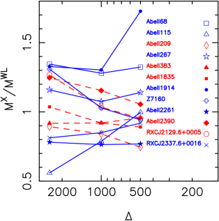
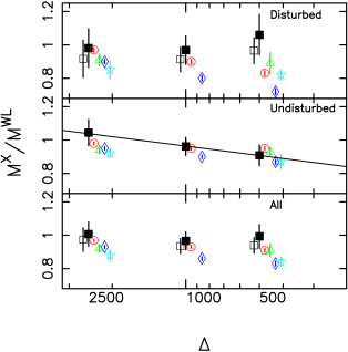
Figure 1.— Left panel : X-ray hydrostatic to weak-lensing mass ratios as a function of density contrast for individual clusters, in which red dashed and blue solid lines denote undisturbed and disturbed clusters, respectively. Right panel: X-ray to weak-lensing mass ratios for all clusters (bottom), undisturbed clusters (middle), and disturbed clusters (top) from our sample including (filled black boxes) and excluding (open black boxes) A1914, together with the X-ray hydrostatic mass to true mass ratios from numerical simulations (PVge2keV, red circles using $T_{\rm MW}$, blue diamonds using $T_{\rm SL}$; Lau et al. 2009, green triangles using quasi-$T_{\rm MW}$; Nagai et al. 2007, light blue stars using $T_{\rm SL}$). The data points at each density contrast are off by 0.022 dex for clarity. We also show the best fit of the X-ray hydrostatic to weak-lensing mass ratio as a function of density contract for the five undisturbed clusters, $M^{\rm X}/M^{\rm WL}=(0.908\pm 0.004)+(0.187\pm 0.010)\cdot\log_{10}(\Delta/500)$. (A color version of this figure is available in the online journal.)

Figure 2.— Normalized histograms of $(M^{\rm X}-M^{\rm WL})/M^{\rm WL}$ for all 12 clusters at $\Delta=2500$ (left panel), $\Delta=1000$ (middle panel), and $\Delta=500$ (right panel).

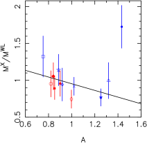
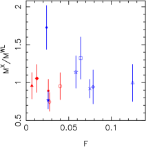
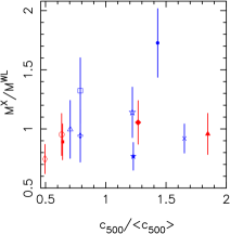
Figure 3.— X-ray hydrostatic to weak-lensing mass ratio at $\Delta=500$ vs. asymmetry parameter (left panel), fluctuation parameter (middle panel), and $c_{500}/\langle c_{500}\rangle$ (right panel), respectively. The colors and symbols are the same as shown in the left panel of Figure 1. The best fit with equal weighting of all data points except for A1914 (the top rightmost point) is shown in the left panel. (A color version of this figure is available in the online journal.)

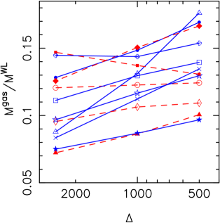
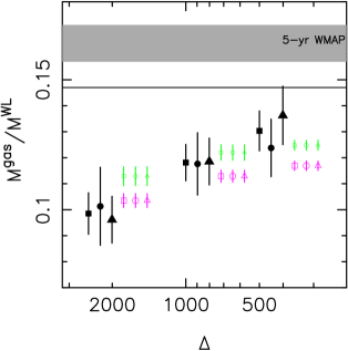
Figure 4.— Left panel: gas mass fractions using weak-lensing masses for individual clusters. The colors, lines, and symbols are the same as shown in the left panel of Figure 1. Right panel: average gas mass fractions using weak-lensing masses (filled symbols). Boxes, circles, and triangles denote all, undisturbed, and disturbed clusters. The data sets are off by 0.048 dex at each density contrast for clarity. The gray horizontal band shows the $1\sigma$ range of the cosmic mean baryon fraction from WMAP five-year data, $\Omega_{\rm b}/\Omega_{\rm m}=0.164\pm 0.007$, in Komatsu et al. (2009), and the black horizontal line corresponds to $0.9\times$ the mean cosmic baryon fraction. Also shown are the gas mass fractions for the sub-samples drawn from the PVge2keV sample with mass cuts of $M_{500}\geq 5\times 10^{14}M_{\odot}$ (small green open symbols) and $M_{500}\geq 2.6\times 10^{14}M_{\odot}$ (big magenta open symbols). (A color version of this figure is available in the online journal.)

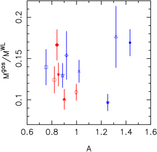
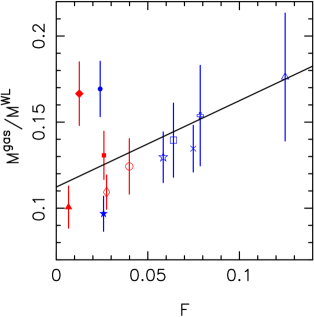
Figure 5.— Gas mass to weak-lensing mass ratio at the radius with $\Delta=500$ vs. asymmetry parameter (left panel) and fluctuation parameter (right panel). The best fit with equal weighting of each data point is shown in the right panel. The colors and symbols are the same as shown in the left panel of Figure 1. (A color version of this figure is available in the online journal.)

Table 1Cluster centers from weak-lensing and X-ray analysis

Cluster Name	X-ray Center [J2000]		Weak-lensing Center [J2000]		Offset		X-ray Morphology
	R.A.	Decl.	R.A.	Decl.	(arcmin)	$r_{2500}$
A68	00 37 06.2	09 09 28.7	00 37 06.9	09 09 24.5	0.18	0.10	Disturbed
A115 (south)	00 56 00.3	26 20 32.5	00 56 00.3	26 20 32.5	0.00	0.00	Disturbed
A209	01 31 52.6	-13 36 35.5	01 31 52.5	-13 36 40.5	0.08	0.04	Undisturbed
A267	01 52 42.0	01 00 41.2	01 52 41.9	01 00 25.7	0.26	0.14	Disturbed
A383	02 48 03.3	-03 31 43.6	02 48 03.4	-03 31 44.7	0.03	0.01	Undisturbed
A1835	14 01 01.9	02 52 35.5	14 01 02.1	02 52 42.8	0.13	0.06	Undisturbed
A1914	14 26 00.9	37 49 38.8	14 25 56.7	37 48 59.2	1.22	0.44	Disturbed
Z7160	14 57 15.2	22 20 31.2	14 57 15.1	22 20 35.3	0.07	0.05	Disturbed
A2261	17 22 26.9	32 07 47.4	17 22 27.2	32 07 57.1	0.34	0.13	Disturbed
A2390	21 53 37.1	17 41 46.4	21 53 36.8	17 41 43.3	0.08	0.03	Undisturbed
RXCJ2129.6+0005	21 29 39.8	00 05 18.5	21 29 40.0	00 05 21.8	0.07	0.04	Undisturbed
RXCJ2337.6+0016	23 37 37.8	00 16 15.5	23 37 39.7	00 16 17.0	0.48	0.25	Disturbed

Note. Within the sample, A1914 and RXCJ2337.6+0016 show extreme offsets between the X-ray and weak-lensing determined cluster central positions. Therefore, the X-ray analysis of the two clusters was revised using the weak-lensing determined cluster centers.

Table 2Cluster mass measurements^a

Cluster Name	$r^{\rm WL}_{2500}$			$r^{\rm WL}_{1000}$			$r^{\rm WL}_{500}$
	$M^{\rm WL}$	$M^{\rm X}$	$M^{\rm gas}$	$M^{\rm WL}$	$M^{\rm X}$	$M^{\rm gas}$	$M^{\rm WL}$	$M^{\rm X}$	$M^{\rm gas}$
A68	$1.42^{+0.59}_{-0.62}$	$1.91\pm 0.57$	$0.158\pm 0.007$	$2.78^{+0.79}_{-0.78}$	$3.56\pm 1.06$	$0.360\pm 0.026$	$4.15^{+1.21}_{-1.06}$	$5.50\pm 1.65$	$0.579\pm 0.057$
A115 (south)	$1.22^{+0.65}_{-0.67}$	$0.68\pm 0.12$	$0.107\pm 0.005$	$2.51^{+0.93}_{-0.91}$	$1.98\pm 0.50$	$0.329\pm 0.017$	$3.85^{+1.61}_{-1.32}$	$3.84\pm 0.99$	$0.679\pm 0.037$
A209	$2.18^{+0.46}_{-0.46}$	$1.95\pm 0.55$	$0.208\pm 0.014$	$5.24^{+0.74}_{-0.72}$	$4.41\pm 1.40$	$0.557\pm 0.050$	$8.81^{+1.31}_{-1.20}$	$6.57\pm 1.95$	$0.963\pm 0.101$
A267	$1.43^{+0.25}_{-0.25}$	$1.66\pm 0.45$	$0.139\pm 0.007$	$2.41^{+0.42}_{-0.40}$	$2.58\pm 0.86$	$0.281\pm 0.021$	$3.29^{+0.68}_{-0.61}$	$3.75\pm 1.16$	$0.426\pm 0.039$
A383	$1.76^{+0.21}_{-0.20}$	$1.61\pm 0.48$	$0.127\pm 0.008$	$2.64^{+0.43}_{-0.40}$	$2.42\pm 0.72$	$0.227\pm 0.022$	$3.38^{+0.71}_{-0.62}$	$3.23\pm 0.95$	$0.340\pm 0.041$
A1835	$2.88^{+0.57}_{-0.58}$	$2.98\pm 0.89$	$0.423\pm 0.023$	$6.15^{+0.95}_{-0.90}$	$5.66\pm 1.68$	$0.844\pm 0.080$	$9.65^{+1.70}_{-1.51}$	$8.59\pm 2.50$	$1.261\pm 0.154$
A1914	$2.09^{+0.31}_{-0.31}$	$2.78\pm 0.76$	$0.268\pm 0.015$	$3.35^{+0.50}_{-0.47}$	$4.36\pm 1.22$	$0.497\pm 0.038$	$4.46^{+0.75}_{-0.69}$	$7.69\pm 2.24$	$0.754\pm 0.066$
Z7160	$0.89^{+0.38}_{-0.42}$	$1.17\pm 0.35$	$0.129\pm 0.004$	$1.75^{+0.58}_{-0.55}$	$1.80\pm 0.52$	$0.251\pm 0.014$	$2.61^{+0.97}_{-0.82}$	$2.46\pm 0.72$	$0.401\pm 0.033$
A2261	$3.55^{+0.44}_{-0.44}$	$2.77\pm 0.75$	$0.266\pm 0.026$	$5.95^{+0.74}_{-0.71}$	$4.54\pm 1.20$	$0.516\pm 0.065$	$8.12^{+1.23}_{-1.12}$	$6.24\pm 1.65$	$0.786\pm 0.114$
A2390	$3.14^{+0.44}_{-0.43}$	$3.92\pm 1.15$	$0.395\pm 0.031$	$5.22^{+0.82}_{-0.77}$	$6.02\pm 1.94$	$0.785\pm 0.083$	$7.09^{+1.29}_{-1.17}$	$7.48\pm 2.22$	$1.180\pm 0.150$
RXCJ2129.6	$1.38^{+0.53}_{-0.54}$	$1.75\pm 0.52$	$0.166\pm 0.009$	$2.97^{+0.69}_{-0.71}$	$3.07\pm 0.93$	$0.364\pm 0.031$	$4.68^{+1.09}_{-0.97}$	$4.46\pm 1.29$	$0.581\pm 0.065$
RXCJ2337.6	$2.42^{+0.36}_{-0.37}$	$1.97\pm 0.44$	$0.202\pm 0.015$	$3.72^{+0.50}_{-0.47}$	$3.16\pm 0.68$	$0.418\pm 0.045$	$4.85^{+0.75}_{-0.70}$	$4.45\pm 0.97$	$0.652\pm 0.084$

Note. ^a The values are in units of $10^{14}$ solar mass.

Table 3Comparison of X-ray and weak-lensing mass estimates

Sample	$M^{\rm X}/M^{\rm WL}$
	$r^{\rm WL}_{2500}$	$r^{\rm WL}_{1000}$	$r^{\rm WL}_{500}$
All	$1.01\pm 0.07$	$0.97\pm 0.05$	$0.99\pm 0.07$
Undisturbed	$1.04\pm 0.08$	$0.96\pm 0.05$	$0.91\pm 0.06$
Disturbed	$0.98\pm 0.12$	$0.97\pm 0.09$	$1.06\pm 0.12$
All-A1914	$0.97\pm 0.07$	$0.94\pm 0.05$	$0.94\pm 0.05$
Disturbed-A1914	$0.92\pm 0.11$	$0.91\pm 0.07$	$0.97\pm 0.08$

Table 4Results of Monte Carlo simulations^a

Sample	$M^{\rm X}/M^{\rm WL}$
	$r^{\rm WL}_{2500}$	$r^{\rm WL}_{1000}$	$r^{\rm WL}_{500}$
All	$1.03\pm 0.09\pm 0.13$	$0.94\pm 0.06\pm 0.05$	$0.95\pm 0.07\pm 0.08$
Undisturbed	$1.02\pm 0.05\pm 0.02$	$0.94\pm 0.04\pm 0.01$	$0.90\pm 0.04\pm 0.02$
Disturbed	$1.05\pm 0.11\pm 0.22$	$0.94\pm 0.07\pm 0.08$	$1.02\pm 0.08\pm 0.11$

Note. ^a The values quoted for each comparison are the mean, standard error, and real variance based on 500 Monte Carlo simulations described in Section 3.1.

Table 5Weak-lensing-based gas mass fractions

Sample	$M^{\rm gas}/M^{\rm WL}$
	$r^{\rm WL}_{2500}$	$r^{\rm WL}_{1000}$	$r^{\rm WL}_{500}$
All	$0.099\pm 0.008$	$0.118\pm 0.007$	$0.130\pm 0.008$
Undisturbed	$0.101\pm 0.015$	$0.118\pm 0.012$	$0.124\pm 0.011$
Disturbed	$0.096\pm 0.009$	$0.119\pm 0.009$	$0.136\pm 0.011$

Table 6X-ray-only gas mass fractions

Sample	$M^{\rm gas}/M^{\rm X}$
	$r^{\rm X}_{2500}$	$r^{\rm X}_{1000}$	$r^{\rm X}_{500}$
All	$0.101\pm 0.010$	$0.118\pm 0.015$	$0.131\pm 0.015$
Undisturbed	$0.100\pm 0.017$	$0.122\pm 0.028$	$0.124\pm 0.023$
Disturbed	$0.101\pm 0.018$	$0.115\pm 0.024$	$0.110\pm 0.026$

References

- Allen (1998) Allen, S. W. 1998, MNRAS, 296, 392
- Allen et al. (2004) Allen, S. W., Schmidt, R. W., Ebeling, H., Fabian, A. C., & van Speybroeck, L. 2004, MNRAS, 353, 457
- Allen et al. (2008) Allen, S. W., et al. 2008, MNRAS, 383, 879
- Balogh et al. (2006) Balogh, M.L., et al. 2006, MNRAS, 366, 624
- Bardeau et al. (2007) Bardeau, S., et al. 2007, A&A, 470, 449
- Boggs et al. (1987) Boggs, P. T., Byrd, R. H., & Schnabel, R. B. 1987, SIAM J. Sci. Stat. Comput., 8, 1052
- Böhringer et al. (2004) Böhringer, H., et al. 2004, A&A, 425, 367
- Bryan (2000) Bryan, G.L. 2000, ApJ, 544, L1
- Clowe et al. (2000) Clowe, D., Luppino, G. A., Kaiser, N., & Gioia, I. M. 2000, ApJ, 539, 540
- Conselice (2003) Conselice, C. J., 2003, ApJS, 147, 1
- Dahle (2006) Dahle, H. 2006, ApJ, 653, 954
- Ebeling et al. (2004) Ebeling, H., et al. 2000, MNRAS, 318, 333
- Ettori et al. (2006) Ettori, S., Dolag, K., Borgani, S., & Murante, G. 2006, MNRAS, 365, 1021
- Evrard (1990) Evrard, A., E., 1990, ApJ, 363, 349
- Fabian et al. (2008) Fabian, A. C., et al. 2008, Nature, 454, 968
- Fahlman et al. (1994) Fahlman, G., Kaiser, N., Squires G., & Woods, D. 1994, ApJ, 437, 56
- Gastaldello et al. (2007) Gastaldello, F., et al. 2007, ApJ, 669, 158
- Gonzalez et al. (2007) Gonzalez, A.H., Zaritsky, D., & Zabludoff, A.I. 2007, ApJ, 666,147
- Haines et al. (2009a) Haines, C. P., et al. 2009a, ApJ, 704, 126
- Haines et al. (2009b) Haines, C. P., et al. 2009b, MNRAS, 396, 1297
- Henry et al. (2009) Henry, J. P., Evrard, A.E., Hoekstra, H., Babul, A., & Mahdavi, A. 2009, ApJ, 691, 1307
- Hoekstra et al. (2001) Hoekstra, H. 2001, A&A, 370, 743
- Ilbert et al. (2009) Ilbert, O., et al. 2009, ApJ, 690, 1236
- Jeltema et al. (2008) Jeltema, T. E., Hallman, E. J., Burns, J. O., & Motl, P. M. 2008, ApJ, 681, 167
- Kay et al. (2007) Kay, S. T., et al. 2007, MNRAS, 377, 317
- Komatsu et al. (2009) Komatsu, E., et al. 2009, ApJS, 180, 330
- Kravtsov et al. (2005) Kravtsov, A. V., Nagai, D., & Vikhlinin, A. 2005, ApJ, 625, 588
- Lau et al. (2009) Lau, E. T., Kravtsov, A. V., & Nagai, D. 2009, ApJ, 705, 1129
- Leauthaud et al. (2010) Leauthaud, A., et al. 2010, ApJ, 709, 97
- Lewis et al. (2000) Lewis, G. F., et al. 2000, ApJ, 536, 623
- Mahdavi et al. (2008) Mahdavi, A., Hoekstra, H., Babul, A., & Henry, J. P. 2008, MNRAS, 384, 1567
- Mantz et al. (2010) Mantz, A., Allen, S.W., Rapetti, D., & Ebeling, H. 2010, MNRAS, submitted, arXiv: 0909.3098
- Marrone et al. (2009) Marrone, D. P., et al. 2009, ApJ, 701, L114
- Mazzotta et al. (2004) Mazzotta, P., Rasia, E., Moscardini, L., & Tormen, G. 2004, MNRAS, 354, 10.
- Meneghetti et al. (2008) Meneghetti, M., et al. 2008, A&A, 482, 403
- Meneghetti et al. (2010) Meneghetti, M., et al. 2010, A&A, in press (arXiv:0912.1343)
- Miniatti et al. (2001) Miniati, F., Ryu, D., Kang, H., & Jones, T. W. 2001, ApJ, 559, 59
- Miniatti (2003) Miniati, F. 2003, MNRAS, 342, 1009
- Miralda-Escude & Babul (1995) Miralda-Escude, J., & Babul, A. 1995, ApJ, 449, 18
- Nagai et al. (2007) Nagai, D., Vikhlinin, A., & Kravtsov, A. V. 2007, ApJ, 655, 98
- Navarro et al. (1997) Navarro, J. F., Frenk, C. S., & White, S. D. M. 1997, ApJ, 490, 493
- Neto et al. (2007) Neto, A.F., et al. 2007, MNRAS, 381, 1450
- Okabe et al. (2010a) Okabe, N., Takada, M., Umetsu, K., Futamase, T., & Smith, G. P. 2010a, PASJ, submitted (arXiv:0903.1103)
- Okabe & Umetsu (2008) Okabe, N., & Umetsu, K. 2008, PASJ, 60, 345
- Okabe et al. (2010b) Okabe, N., et al. 2010b, ApJ, submitted
- Pfrommer et al. (2007) Pfrommer, C., Enßlin, T. A., Springel, V., Jubelgas, M., & Dolag, K. 2007, MNRAS, 378, 385
- Piffaretti et al. (2008) Piffaretti, R., & Valdarnini, R. 2008, A&A, 491, 71
- Poole et al. (2006) Poole, G. B., et al. 2006, MNRAS, 373, 881
- Pratt et al. (2009) Pratt, G. W., Croston, J. H., Arnaud, M., & Böhringer, H., 2009, A&A, 498, 361
- Rasia et al. (2006) Rasia, E., et al. 2006, MNRAS, 369, 2013
- Richard et al. (2009) Richard, J., et al. 2010, MNRAS, in press (arXiv:0911.3302)
- Sanderson et al. (2009) Sanderson, A.J.R., Edge, A. C., & Smith, G.P. 2009, MNRAS, 398, 1698
- Sanderson & Ponman (2010) Sanderson, A.J.R., & Ponman, T.J. 2010, MNRAS, in press (arXiv:0910.3212)
- Squires et al. (1996) Squires, G., et al. 1996, ApJ, 461, 572
- Umetsu et al. (2009) Umetsu, K., et al. 2009, ApJ, 694, 1643
- Valdarnini et al. (2003) Valdarnini, R. 2003, MNRAS, 339, 1117
- Vikhlinin et al. (2002) Vikhlinin, A., van Speybroeck, L., Markevitch, M., Forman, W., & Grego, L. 2002, ApJ, 578, L107
- Vikhlinin et al. (2006) Vikhlinin, A., et al. 2006, ApJ, 640, 691
- Vikhlinin et al. (2009a) Vikhlinin, A., et al. 2009a, ApJ, 692, 1033
- Vikhlinin et al. (2009b) Vikhlinin, A., et al. 2009b, ApJ, 692, 1060
- White et al. (1993) White, S. M., Navarro, J. F., Evrard, A. E., & Frenk, C. S. 1993, Nature, 336, 429
- Wu & Fang (1996) Wu, X.-P., & Fang, L.-Z. 1996, ApJ, 467, L45
- Zhang et al. (2005) Zhang, Y.-Y., Böhringer, H., Mellier, Y., Soucail, G., Forman, W. 2005, A&A, 429, 85
- Zhang et al. (2009) Zhang, Y.-Y., Reiprich, T. H., Finoguenov, A., Hudson, D. S., & Sarazin, C. L., 2009, ApJ, 699, 1178
- Zhang & Wu (2003) Zhang, Y.-Y., & Wu, X.-P. 2003, ApJ, 583, 529
- Zhang et al. (2006) Zhang, Y.-Y., et al. 2006, A&A, 456, 55
- Zhang et al. (2007) Zhang, Y.-Y., et al. 2007, A&A, 467, 437
- Zhang et al. (2008) Zhang, Y.-Y., et al. 2008, A&A, 482, 451