A Streamwise Constant Model of Turbulence in Plane Couette Flow

Abstract

Streamwise and quasi-streamwise elongated structures have been shown to play a significant role in turbulent shear flows. We model the mean behavior of fully turbulent plane Couette flow using a streamwise constant projection of the Navier Stokes equations. This results in a two-dimensional, three velocity component ($2D/3C$) model. We first use a steady state version of the model to demonstrate that its nonlinear coupling provides the mathematical mechanism that shapes the turbulent velocity profile. Simulations of the $2D/3C$ model under small amplitude Gaussian forcing of the cross-stream components are compared to DNS data. The results indicate that a streamwise constant projection of the Navier Stokes equations captures salient features of fully turbulent plane Couette flow at low Reynolds numbers. A system theoretic approach is used to demonstrate the presence of large input-output amplification through the forced $2D/3C$ model. It is this amplification coupled with the appropriate nonlinearity that enables the $2D/3C$ model to generate turbulent behaviour under the small amplitude forcing employed in this study.

1 Introduction

The Navier Stokes (NS) equations provide a complete dynamical description of the three velocity components and pressure for simple canonical flows under the sole modeling assumption that all important physical phenomena are captured by these equations. Unfortunately, these infinite dimensional algebraically constrained equations are analytically intractable. They have however, been extensively studied computationally and numerical solutions do exist. For plane Couette flow, the first numerical solution was computed by Nagata (1990). Gibson et al. (2009) provide a detailed discussion of other work related to a full range of numerical plane Couette flow solutions. Ever increasing computing power will continue to allow progress toward understanding these local properties. However, a full mathematical understanding of NS even in simple parallel flow configurations remains elusive, hence considerable effort has been applied to the search for more analytically-tractable flow models.

In contrast, the Linearized Navier Stokes (LNS) equations can be analyzed using well developed tools from linear systems theory. For wall bounded shear flows, one particular property of the LNS that has been extensively studied is disturbance amplification, e.g. Farrell (1988); Gustavsson (1991); Reddy & Henningson (1993); Farrell & Ioannou (1993b); Bamieh & Dahleh (2001); Jovanović & Bamieh (2005). Large disturbance amplification is common in these flows because the linear operators governing them are non-normal, (i.e., the operator, $A$, is such that $A^{*}A\neq AA^{*}$).

The LNS are thought to capture the energy production of the full nonlinear system. Henningson & Reddy (1994) showed that non-normality and linear mechanisms are necessary conditions for subcritical transition to turbulence and it is widely believed that energy amplification is due to coupling terms that remain in linearized models, see for example (Trefethen et al., 1993). In smooth wall-bounded shear flows the linear coupling between the Orr-Sommerfeld and Squire equations associated with nonzero spanwise wave number has been shown to be required for the generation of the wall layer streaks that are necessary to maintain turbulence (Butler & Farrell, 1993; Kim & Lim, 2000). In this context, the term “streak” describes the “well-defined elongated region of spanwise alternating bands of low and high speed fluid” (Waleffe et al., 1991). The LNS have also been used by Jovanović & Bamieh (2001) to predict certain second-order statistics of turbulent channel flow. The above results and a host of others illustrate the power of the LNS as a model for wall-bounded shear flows. There is however, one fundamental flow feature that linear models are unable to capture; the change in the mean velocity profile as the flow transitions from laminar to turbulent. In addition, linear analysis can only give local information regarding the full (nonlinear) system.

Empirical models have been shown to be useful in capturing key aspects of many flows. For example, Proper Orthogonal Decomposition (POD) has been successfully used to construct accurate low dimensional ordinary differential equation models, e.g. (Lumley, 1967; Smith et al., 2005). However the preceding analysis utilizes existing experimental or numerical data, a limitation also applicable to eddy viscosity models. In general, data-driven or heuristic models can be said to suffer from a lack of connection, of varying degree, to the governing equations of the problem.

The model studied herein is an attempt to merge the benefits of studying a physics-based set of equations, such as NS, with the analytical tractability of a simplified model, such as the LNS. It is developed based on the assumption that certain aspects of fully developed turbulent flow can be reasonably modeled as homogeneous in the streamwise direction, here denoted “streamwise constant”. The idea that a streamwise constant model is sufficient to capture mean profile changes from laminar to turbulent is strongly supported by the work of Reddy & Ioannou (2000), who showed that nonlinear interaction between the $(k_{x},k_{z})=(0,\pm N)$ modes, where the $k$’s are the streamwise and spanwise wave numbers, is the primary factor in determining the turbulent mean velocity profile in Couette flow. Further, as was discussed in Orlandi & Jiménez (1994), this type of model may be adequate to capture many of the effects associated with the generation of turbulent wall friction. A $2\frac{1}{2}$D model along similar lines has also been developed for the viscous wall layer; Tullis & Pollard (1993) for example use such a model to study flow over riblets in this region. The physical and analytical basis for assuming homogeneity in the streamwise direction is discussed in the following section.

1.1 Streamwise Coherence

A growing body of work supports the notion that turbulence in wall-bounded shear flows is characterized by dynamically significant coherent structures, particularly features with streamwise and quasi-streamwise alignment. Near-wall streaks (Kline et al., 1967), for example, have been shown to play a key role in energy production through the ‘near-wall autonomous cycle’ discussed by Waleffe (1990); Hamilton et al. (1995); Waleffe (1997); Jiménez & Pinelli (1999). This cycle is generally agreed to be an important mechanism in determining the low-order statistics of turbulent flows in the buffer region and viscous sublayer, i.e. $y^{+}\leq 30$ (Schoppa & Hussain, 2002).

More recent high Reynolds number studies have focused on the identification and characterization of streamwise coherence in the core, i.e. Kim & Adrian (1999); Morrison et al. (2004); Guala et al. (2006); Hutchins & Marusic (2007a). These motions have been called large and very large scale motions (respectively LSM and VLSMs). They appear to have a similar signature to the near-wall streaks (Hutchins & Marusic, 2007b; Chung & McKeon, 2010), but tend to be longer in extent, from one to ten times the outer length scale, $\delta$. There is experimental evidence to suggest that at high Reynolds numbers (for example $Re_{\tau}>7300$), VLSMs contain more energy than the near-wall structures (Morrison et al., 2004; Hutchins & Marusic, 2007a, b). In turbulent boundary layers they have also been shown to modulate the near-wall turbulence, see for example Hutchins & Marusic (2007b); Mathis et al. (2009), suggesting that they may play an important role in flow dynamics across a range of scales.

In Couette flow, structures reminiscent of VLSMs have long been observed in the core through DNS of turbulent plane Couette flow (Lee & Kim, 1991; Bech et al., 1995). Although some studies raised the concern that the structures were numerical artifacts, recent DNS at higher resolution and with longer box sizes (Komminaho et al., 1996; Tsukahara et al., 2006) have confirmed the existence of long streamwise alternating high and low speed streaky structures at the centerline. In experiments, VLSMs were first identified through observations of a noticeable peak in the Fourier energy spectrum of the turbulence intensity at low frequencies (Komminaho et al., 1996; Kitoh & Umeki, 2008). The Couette flow experiments of Tillmark & Alfredsson (1998) found further evidence of very long structures in the form of long autocorrelations $R_{uu}(\tau)$ and two-point correlations $R_{uu}(\Delta x)$ as well as periodic variation of spanwise correlations $R_{uu}(\Delta z)$ in the core. The streamwise extent of these correlations was longer than those generally seen in other wall-bounded flows. Komminaho et al. (1996) also found that in contrast to other flows, the streamwise correlations for Couette flow are larger at the center than near the wall. At channel center the zero cross distances of $R_{uu}(\tau)$ and $R_{uu}(\Delta x)$ have been observed to be three times that of the corresponding structures in Poiseuille flow (Kitoh et al., 2005). This makes Couette flow an ideal candidate to test the applicability of a streamwise constant model.

Streamwise constant, $k_{x}=0$, perturbations to the LNS also produce the largest input-output response for both laminar (Bamieh & Dahleh, 2001; Jovanović & Bamieh, 2001; Farrell & Ioannou, 1993b, 1998) and turbulent (del Álamo & Jiménez, 2006) base velocity profiles. In addition, streaks of streamwise velocity naturally arise from the set of initial conditions that produce the largest energy growth (Butler & Farrell, 1992; Farrell & Ioannou, 1993a), namely streamwise vortices. Even in linearly unstable flows, studies have shown that the amplitude of streamwise constant structures can exceed that of the linearly unstable modes (Jovanović & Bamieh, 2004; Gustavsson, 1991). For channel flows, Bamieh & Dahleh (2001) explicitly showed that streamwise constant disturbances produce energy growth on the order of $Re^{3}$ whereas streamwise varying disturbances grow as a function of $Re^{\frac{3}{2}}$.

In the present work we employ a streamwise constant model based on the previously discussed experimental and analytical evidence of the importance of streamwise homogenous features. This so-called two-dimensional, three (velocity) component, henceforth $2D/3C$, model for plane Couette flow is simulated under small amplitude Gaussian forcing. The results demonstrate the ability of this model to capture some important features of fully developed turbulent flow. In particular, it is demonstrated that: (1) the nonlinear terms in the $2D/3C$ model capture the momentum redistribution mechanism involved in creating the shape of the turbulent velocity profile, (2) a stochastically forced $2D/3C$ model can reproduce the appropriate turbulent mean velocity profile and Reynolds number trends, and (3) this model produces amplification of small disturbances that is consistent with input-output studies of the LNS. The work is organized as follows: the next sections of the paper describe the model and simulation approach. Results and discussion follow, including a comparison between the model and a DNS dataset, before final conclusions.

2 The $2D/3C$ Model

The $2D/3C$ model discussed herein is obtained by setting streamwise ($x$-direction) velocity derivatives in the full NS equations describing Couette flow to zero (Bobba, 2004). This can be thought of as a projection of the NS into the streamwise constant space. One can explicitly show that for Couette flow this $2D/3C$ formulation also results in a system with zero streamwise pressure gradient.

The velocity field is decomposed such that $\vec{\mathbf{u}}=[U+u^{\prime}_{sw};V+v^{\prime}_{sw},W+w^{\prime}_{sw}]$; where $U=U(y)=y,\;V=W=0$ is the laminar Couette flow and $(u^{\prime}_{sw},v^{\prime}_{sw},w^{\prime}_{sw})$ are the corresponding time-dependent deviations from laminar in the streamwise constant sense.

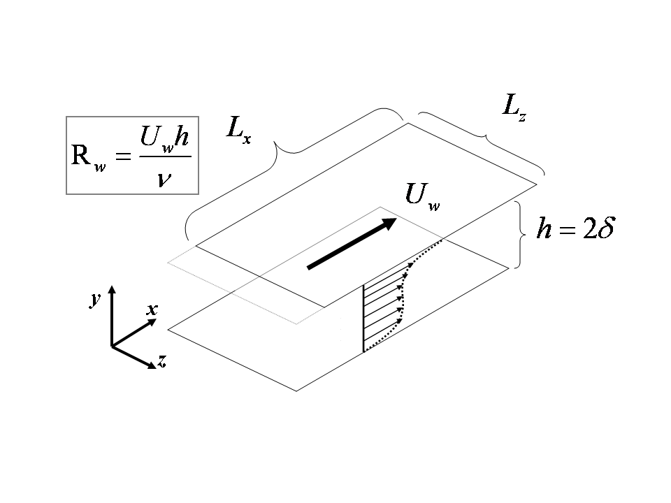
Figure 1: Flow geometry. Streamwise and spanwise boundaries are periodic, the bottom wall is stationary and the top wall moves in the $x$-direction with a velocity $U_{w}$. The channel half height is denoted $\delta$ and the full channel height is denoted $h$.

The flow geometry is shown in Figure 1. The Reynolds number employed is $Re_{w}=\frac{U_{w}h}{\nu}$, where $U_{w}$ is the velocity of the top plate, $h$ is the channel height and $\nu$ is the kinematic viscosity of the fluid. All distances and velocities are respectively normalized by $h$ and $U_{w}$. In the sequel we will use $(u^{\prime}_{sw},v^{\prime}_{sw},w^{\prime}_{sw})$ to denote $\left(\frac{u^{\prime}_{sw}}{U_{w}},\frac{v^{\prime}_{sw}}{U_{w}},\frac{w^{\prime}_{sw}}{U_{w}}\right)$, and explicitly indicate the scaling only in the figure labels.

A stream function

$$v^{\prime}_{sw}=\frac{\partial\psi}{\partial z};\;\quad w^{\prime}_{sw}=-\frac{\partial\psi}{\partial y}$$

forces the appropriate $2D$ continuity. This results in the following model:

$$\frac{\partial u^{\prime}_{sw}}{\partial t} =-\frac{\partial\psi}{\partial z}\frac{\partial u^{\prime}_{sw}}{\partial y}-\frac{\partial\psi}{\partial z}\frac{\partial U}{\partial y}+\frac{\partial\psi}{\partial y}\frac{\partial u^{\prime}_{sw}}{\partial z}+\frac{1}{Re_{w}}\Delta u^{\prime}_{sw}$$ (1)

$$\frac{{\partial\Delta\psi}}{{\partial t}} =-\frac{\partial\psi}{\partial z}\frac{\partial\Delta\psi}{\partial y}+\frac{\partial\psi}{\partial y}\frac{\partial\Delta\psi}{\partial z}+\frac{1}{Re_{w}}\Delta^{2}\psi.$$

No slip boundary conditions at the wall and periodic boundary conditions in the spanwise direction are applied (without loss of generality they can also be used for the stream function equation since $v^{\prime}_{sw}=w^{\prime}_{sw}=0\Rightarrow\frac{\partial\psi}{\partial z}=\frac{\partial\psi}{\partial y}=0\Rightarrow\psi=\mbox{const}$). This model retains many of the important flow features lost in a purely $2D$ model by maintaining all three velocity components. Equations (1) are an improvement over linear models because it is hypothesized that it is the nonlinearity in the $u^{\prime}_{sw}(y,z,t)$ equation that provides the mathematical mechanism for the redistribution of the fluid momentum. This redistribution creates larger streamwise velocity gradients in the wall-normal direction and changes the plane Couette velocity profile from linear to its characteristic turbulent “S-shape”. Meanwhile, the important features of the LNS are maintained. Linearization of (1) around the laminar profile produces a non-normal operator with a coupling term analogous to the one in the LNS.

The laminar flow solution of Equation (1) was previously shown to be globally, that is nonlinearly, stable for all Reynolds numbers (Bobba et al., 2002), and therefore the laminar flow constitutes a unique solution. Consequently any transition mechanisms associated with bifurcations, escape from the basin of attraction of the laminar solution or the like are not possible. So, any complications associated with these nonlinear phenomena can be eliminated from the analysis of these particular equations. Global asymptotic stability of the laminar solution also implies that without forcing, perturbations will eventually decay, in agreement with the results of Orlandi & Jiménez (1994) who found that after an initial perturbation a $2D/3C$ model decays (back to laminar) with time. The fact that one can analytically prove that the unforced $2D/3C$ model has a unique solution suggests that it is far more analytically tractable than NS. We do not pursue analytical studies of the $2D/3C$ model in the current work, but instead concern ourselves with showing the applicability of the model in describing important features of the flow field. However, the fact that global statements about these equations can be made implies that future analytical studies are promising.

As with any model, there are assumptions built into the $2D/3C$ model, and it is important to understand how these relate to the physical phenomena associated with turbulent flows. Most obviously, small scale, three-dimensional turbulent activity, including the specifics of several structures that are known to exist in the full flow, is not captured. While this makes appropriate scaling relationships more difficult to determine, it does not diminish the potential of the model for predicting and understanding key aspects of turbulence in plane Couette flow. The challenge lies in extending the $2D/3C$ model to incorporate aspects of the streamwise variation associated three-dimensional turbulent flow.

2.1 Modeling Framework

No model is a perfect representation of reality. In addition to modeling assumptions, parameter errors or external influences on the system in question are often ignored. Inaccurate parameter estimates or linearization of a nonlinear system may change the model’s ability to predict behavior. Environmental conditions that affect (or disturb) the system may also play an important role in its dynamics. This role is not captured by a typical model.

Robust control theory has historically been used to analyze models in the presence of such modeling errors (‘uncertainty’) Doyle et al. (1991); Zhou et al. (1996). One typically represents all of the uncertainties using an uncertainty operator $\Delta$. The block diagram of Figure 3 is then used to depict a model subject to this uncertain set $\Delta$. Generally robust control tools provide a bound on $\|\Delta\|$, below which a desired property can be maintained. Robust control tools do not require a detailed model of the particular uncertainty. This makes them appealing in situations where there are unknown (or hard to model) environmental influences on the system, or when one can only specify the range on a parameter, rather than an exact value. However, since the uncertainty is generally specified through a bound that includes the worst case scenario, the results of this type of analysis may be very conservative. One way to mitigate this is to ‘structure’ or shape the uncertainty, a process which relies on some understanding of the implicit modeling errors.

Figure 2: A robust control block diagram for a model subject to uncertainty. Generally a norm bound on $\Delta$ specifies the amount of uncertainty that a model can have before a desired property is lost (i.e., if the model is stable for $\|\Delta\|\leq 1$, this implies robust stability).

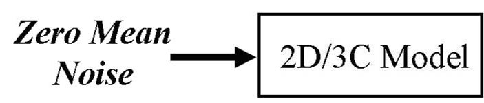
Figure 3: The approximation for illustrating the $2D/3C$ model’s lack of robustness. The zero-mean noise as an approximation for the modeling errors and uncertainty. The noise acts as an additive “uncertainty” at each time step.

In the context of a system comprising a wall-bounded shear flow, many disturbances can be modeled through the $\Delta$ block in Figure 3. These sources of modeling errors (uncertainties) can arise from assumptions on the boundary conditions or unmodeled dynamics. External sources of model uncertainty that are not captured in the NS equations, include phenomena such as acoustic noise and thermal fluctuations in an experiment, or the build up of numerical error in simulations. In addition the uncertain set includes terms excluded by the modeling assumptions, namely the $k_{x}\neq 0$ modes in the $2D/3C$ model, or the nonlinear terms for the LNS model. See Bobba (2004) for a full characterization of the types of uncertainties present in shear flow problems. Obviously the latter class of perturbations are strictly bound to satisfy the NS equations, while the former are less constrained. Distributed wall roughness (i.e., surface imperfections present in any real surface), wall vibration, imperfect alignment of the walls or other parameter estimates may be captured through either stochastic or other forcing.

In the present work, the framework of robust control is employed in a nontraditional manner. Instead of providing an upper bound on $\|\Delta\|$, (i.e. a robustness guarantee) we describe the extent to which the laminar flow state is ‘fragile’ (i.e. unable to be maintained in the face of infinitesimal disturbances). One can think of this as an inverse robustness (or ‘fragility’) problem, i.e. a discussion of a lack of robustness. In order to study the disturbance response of the $2D/3C$ model the system of Figure 3 is abstracted into the simplified setting of Figure 3. We further simplify by linearizing the $\Delta\psi(y,z,t)$ equation which is equivalent to recognizing that advection terms in the stream function equation play a lesser role in redistributing momentum. The forcing and henceforth $\psi$ are constrained to be small such that the nonlinear terms are at least an order of magnitude smaller than the linear ones in all cases studied here. This small amplitude noise assumption is very important in the development of this work because of the focus on the effect of small amplitude disturbances on a fragile system and because larger amplitude forcing can change the dynamics of the model.

For all of the numerical studies described herein we simulate

$$\frac{\partial u^{\prime}_{sw}}{\partial t} =-\frac{\partial\psi}{\partial z}\frac{\partial u^{\prime}_{sw}}{\partial y}-\frac{\partial\psi}{\partial z}\frac{\partial U}{\partial y}+\frac{\partial\psi}{\partial y}\frac{\partial u^{\prime}_{sw}}{\partial z}+\frac{1}{Re_{w}}\Delta u^{\prime}_{sw}+d_{u}$$ (2)

$$\frac{\partial\Delta\psi}{\partial t} =\frac{1}{Re_{w}}\Delta^{2}\psi+d_{\psi},$$

with the same boundary conditions as in Equation (1). A short simulation study comparing low-order streamwise velocity statistics supports the use of linearization in the $\psi$ equation.

Approximating the full $3D$ system using the interconnection in Figure 3 would involve nonlinear mixing modes. In order to approximate the range of frequencies associated with the full $3D$ system in the framework of Figure 3, zero mean stochastic forcing was applied to the $2D/3C$ model. In particular, the inputs $d_{u}(y,z,t)$ and $d_{\psi}(y,z,t)$ in (2) are small amplitude and Gaussian, as in Gayme et al. (2009). The input amplitudes are defined using the standard deviation, $\sigma_{noise}$. Note that under these assumptions there is no coupling from the streamwise components ($u$) back to the cross-stream components (the $\Delta\psi$ equation). The plausibility of modeling the type of disturbances common to experimental conditions in this manner is confirmed by results from stochastic forcing of the LNS equations, which leads to flows dominated by streamwise elongated streaks and vortices that are strikingly similar to those observed in experiments (Farrell & Ioannou, 1993b), as well as by the results of the simulation study discussed in Section 4.3. Further development of the model would be required to address this effective feedback mechanism.

3 Approach

Time-dependent simulations of the full coupled system (2) were carried out using a basic second-order central difference scheme in both the spanwise ($z$) and wall-normal ($y$) directions. Periodic boundary conditions in $z$ and no-slip boundary conditions in $y$ were applied. Simulations using the spectral methods of Weideman & Reddy (2000) were also performed for comparison. The pseudospectral simulations employ a Chebyshev interpolant for the wall-normal direction and a Fourier method for the spanwise derivatives. The aspect ratio in all of the simulations was greater than $12$ to $1$ (spanwise to wall-normal) in order to eliminate box size effects; specifically the usual computational box size was $L_{y}\times L_{z}=h\times~{}12.8h$ with $75\times 100$ grid points. A spanwise extent of $12.8h$ was selected to provide a direct comparison to the full field DNS data from Tsukahara et al. (2006).

In this study, the response of the streamwise velocity, $u^{\prime}_{sw}$, to forcing of the cross-stream velocity components, $v^{\prime}_{sw}$ and $w^{\prime}_{sw}$, was examined. A forcing input of zero mean small amplitude Gaussian noise evenly applied at each $y$–$z$ plane grid point was selected for $d_{\psi}$. The other input forcing, $d_{u}$, was set to zero based on previous studies of the LNS, which showed that the response to streamwise body forcing is significantly smaller than the response to spanwise/wall-normal plane forcing (Jovanović & Bamieh, 2005). These studies used an order of magnitude argument to conclude that the difference in response scales as $\frac{1}{Re^{2}}$. Furthermore, it is energy redistribution by streamwise vorticity (i.e. $\Delta\Psi$) that is thought to be the primary effect governing the shape of the turbulent velocity profile (Hamilton et al., 1995). The response in the streamwise velocity component to this forcing may have a nonzero mean because of the nonlinearity in the $u$ equation.

The different discretization techniques naturally provide a comparison of different noise forcing distributions. For example, the Chebyshev grid results in a higher concentration of noise forcing near the walls. Throughout the present work it is assumed that significant numerical errors are not introduced by the methods of discretization, i.e. the introduction of significant noise arises only through the $d$ terms of Equation (1).

The time evolution of $\Delta\psi$ in Equation (2) can be seen to be a stochastically forced heat equation, i.e. a linear stochastic partial differential equation which can be solved analytically (see for example Swanson (2007) or Luo (2006) and the references therein). This is not pursued here because a simulation is a much simpler way to demonstrate the efficacy of the model. An exposition on Itô calculus and Wiener chaos expansions is beyond the scope of this paper. Future work may involve pursuing analytical solutions to both the linear approximation to $\psi$ and the full nonlinear system (1).

4 Results and Discussion

The results will be divided into three main sections. We begin by analyzing the DNS data of Tsukahara et al. (2006) in the light of the $2D/3C$ model and confirming the extent to which the assumptions of the $2D/3C$ model can be adduced through this data. Following that, a time independent version of Equation (1) is studied to verify the implicit model filter between $\psi$ and $u$. Finally, results from full simulations of the time-dependent Equations (2) are presented and compared to the DNS data.

4.1 Comparison of DNS data with $2D/3C$ Modeling Assumptions

Full details of the DNS dataset can be found in Tsukahara et al. (2006); a brief review of key aspects is given here. Three Reynolds numbers were considered, $Re_{w}=3000,8600$ and $12800$, all with computational domain size $L_{x}\times L_{y}\times L_{z}=44.8h\times h\times 12.8h$, $1024\times 96\times 512$ grid points, and a sampling time ($\frac{tU_{w}}{L_{x}}$) of $91$. The fourth-order finite difference scheme proposed in Morinishi (1995) was employed for the $x$ and $z$ directions. A second-order finite difference method was used for the $y$ direction.

The friction coefficient, $C_{f}=9.59\times 10^{-3}$, is somewhat higher than in other studies, such as Robertson & Johnson (1970). Filling this friction factor into the relationship developed by Robertson (1959),

$$\sqrt{\frac{{C_{f}}}{2}}=\frac{G}{{\log_{10}\left({\raise 2.15277pt\hbox{$\scriptstyle 1$}\kern-1.00006pt/\kern-1.49994pt\lower 1.07639pt\hbox{$\scriptstyle 4$}}Re_{w}\right)}}\quad\mbox{ where }\quad C_{f}=\frac{{\tau_{w}}}{{\raise 2.15277pt\hbox{$\scriptstyle 1$}\kern-1.00006pt/\kern-1.49994pt\lower 1.07639pt\hbox{$\scriptstyle 2$}}\;\rho\left({\raise 2.15277pt\hbox{$\scriptstyle 1$}\kern-1.00006pt/\kern-1.49994pt\lower 1.07639pt\hbox{$\scriptstyle 2$}}U_{w}\right)^{2}}$$ (3)

with $\tau_{w}$ used to denote shear stress at the wall, leads to an experimental constant $G=0.199$. Other values reported in the literature include $G=0.19$ and $G=0.174$ both from Robertson (1959) based on the data of Reichardt and Robertson respectively and $G=0.182$ from the experimental study of El Telbany & Reynolds (1982).

The turbulent mean velocity profiles, turbulence intensities, Reynolds stresses and budgets of $\overline{u^{\prime}_{i}u^{\prime}_{j}}$ from this DNS show good agreement with the experimental results of Tillmark (1995) and the spectral DNS study of Komminaho et al. (1996) which used a larger box. The two-point correlations in $u$ indicate that the box lengths used in both the streamwise, $R_{uu}(\Delta x)$, and spanwise, $R_{uu}(\Delta z)$, directions are sufficient to eliminate any boundary condition-related spurious effects.

In what follows, a streamwise constant projection of the DNS data is approximated through a streamwise ($x$) average over the box length, which will highlight streamwise coherence of the order of the box length. The $x$-averaged DNS data is denoted $\vec{\mathbf{u}_{x_{ave}}}=(u^{\prime}_{x_{ave}}+U(y),v^{\prime}_{x_{ave}},w^{\prime}_{x_{ave}})$ to distinguish it from true streamwise constant data. Time averages are indicated by an overbar, $\overline{({\cdot})}$.

The ratio of the energy contained in the $x$-averaged DNS to that of the full field provides a quantitative measure of the extent to which the DNS data can be approximated as streamwise constant. For this comparison the squared $2$-norm is used to approximate the energy in each $2$-dimensional $x$-averaged velocity component

$$\|\beta\|^{2}= \int_{\mathcal{Z}}\int_{0}^{1}\beta(y,z)^{2}\,dy\;dz$$ (4)

$$\approx \frac{\Delta z}{2L_{y}\;L_{z}}\sum_{k=1}^{N_{z}-1}\left(\sum_{j=1}^{N_{y}-1}\frac{\Delta y_{j+1}}{2}\left[\beta^{2}(y_{j+1},z_{k+1})+\beta^{2}(y_{j},z_{k+1})+\right.\right.$$

$$\hskip 177.82971pt+\left.\left.\beta^{2}(y_{j+1},z_{k})+\beta^{2}(y_{j},z_{k})\right]\right),$$

where $\mathcal{Z}$ is the spanwise extent, $\Delta z=z_{2}-z_{1}$ is the spanwise distance between $z$ grid points and trapezoidal approximations are used for the inhomogeneous $y$ grid.

Component	Total Energy Norm	Percent of Total Energy
	$\|\cdot\|$	in $x$-averaged Norm
$u$	0.5334	99.1
$u-U$	0.1686	90.2
$v$	0.0279	19.0
$w$	0.0412	15.0

Table 1: Energy content in the $x$-averaged DNS velocity components at $Re_{w}=3000$.

Table 1 shows the total energy (based on the full DNS field at $Re_{w}=3000$) and the percentage contained in each of the $x$-averaged velocity components ($u,\,v,\,w$) as well as in the deviation from laminar (denoted $u-U$). This latter quantity is most representative of the energy associated with the differences in the mean velocity profile for a turbulent versus a laminar flow. The computations show that $x$-averaged streamwise velocity contains $99\%$ of the ($u$) energy, whereas the corresponding deviation from laminar contains $90\%$. As expected, the $x$-averaging results in a larger loss of information in the spanwise and wall-normal velocity components.

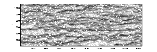
Figure 4: An $z$–$x$ plane contour plot of the streamwise velocity, $u$, from the DNS field, (bottom up view) at $y^{+}=29$. Light colored contours denote regions of higher velocity and dark contours indicate lower velocity regions.

An examination of the DNS streamwise velocity field at $y^{+}=29$, close to the outer edge of the region affected by the near-wall cycle, reveals the signature of streamwise elongated, large scale streaks in the streamwise/wall-normal plane of the full field (Figure 4). These streaks are also visible in Figures 5(a) and 5(b) which depict contour plots of the deviation from laminar flow, $u^{\prime}_{x_{ave}}=u_{x_{ave}}-U$, when averaged over $25\%$ of the streamwise field and the full field respectively. Clearly, increasing the averaging length acts as a filter on structures of different streamwise extent. The average over the full box length retains strong evidence of structures across the entire spanwise/wall-normal plane. In particular, the strongest signature near the wall is in qualitative agreement with the near-wall model of energetic structures centered around $y^{+}\approx 15$ with a statistical diameter of $y^{+}\sim 30$. Another important feature of Figure 5(b) is that the maximum deviations from laminar flow, which are out of spatial phase with one another, top to bottom, are associated with large-scale rolling motions which reach across the channel height.

(a) Average over $25\%$ of streamwise box

(b) Average over full streamwise box

Figure 5: $y$–$z$ plane contour plots of the $x$-averaged (as an approximation for streamwise constant) DNS deviations from laminar ($u_{{x}_{ave}}^{\prime}$) (a) averaged over $25\%$ of the streamwise box length and (b) averaged over the full streamwise box length.

The above analysis shows that there is good agreement between the DNS data and our assumptions. In the next section this data is used to suggest a time-independent model for $\psi(y,z)$ in order to study a steady state version of the streamwise velocity in (1). This is followed by simulation of the full system (2).

4.2 Time Independent $u_{x}(y,z,t)$ Equation

The response of Equation 1 to a stream function that is independent of time, $\psi_{ss}(y,z)$, is of interest for two reasons: (1) the forced solution for the streamwise velocity permits investigation of whether the $2D/3C$ model filters an appropriately shaped $\psi_{ss}(y,z)$ towards the expected shape of the turbulent velocity profile, and (2) it gives insight into the mathematical mechanisms that create the momentum (energy) transfer that generates the blunted profile. The analysis constitutes a weakly nonlinear analysis, in which the time-independent forcing takes the form $\psi_{ss}=\psi_{{ss}_{0}}+\varepsilon\psi_{{ss}_{1}}+\dots$.

In Barkley & Tuckerman (2007) it was shown that laminar-turbulent flow patterns in plane Couette flow could be reproduced using a stream function of the form $\psi(y,z)=\psi_{0}(y)+\psi_{1}(y)\cos(k_{z}z)+\psi_{2}(y)\sin(k_{z}z)$. We use this study as guidance but set the zeroth-order term $\psi_{0}$ to zero because a nonzero $\psi_{0}$ produces a nonzero-mean spanwise flow $w^{\prime}_{ss}$, which is not representative of the velocity field we are interested in studying. The DNS field (Tsukahara et al., 2006) was also used as a guide to ensure that the first-order term $\psi_{{ss}_{1}}$ as well as the corresponding wall-normal and spanwise velocities, respectively $v_{{ss}_{1}}^{\prime}$ and $w_{{ss}_{1}}^{\prime}$, contained representative features. For ease of computation and analysis a simple analytic model for $\psi_{{ss}_{1}}(y,z)$ was selected, namely a doubly-harmonic model which matches the boundary conditions

$$\psi_{ss}=\varepsilon\psi_{{ss}_{1}}(y,z)=\varepsilon\sin^{2}\left({\pi y}\right)\cos\left({\frac{{2\pi}}{{\lambda_{z}}}z}\right).$$ (5)

This corresponds to

$$v^{\prime}_{{ss}_{1}}(y,z)=-\frac{2\pi}{\lambda_{z}}\sin^{2}\left({\pi y}\right)\sin\left({\frac{{2\pi}}{{\lambda_{z}}}z}\right),\mbox{ and }w^{\prime}_{{ss}_{1}}(y,z)=-\pi\sin\left({2\pi y}\right)\cos\left({\frac{{2\pi}}{{\lambda_{z}}}z}\right).$$

The size of the perturbation, $\varepsilon$, is a free variable to be explored, while the spanwise wavelength, $\lambda_{z}$, is fixed to a value determined using the DNS data.

Streamwise averages of both $v(x,y,z)$ and $w(x,y,z)$ from the DNS data permit an estimate of $\psi_{{ss}}(y,z)$, (to within some constant), for that particular field. A contour plot of the approximation based on $w^{\prime}_{x_{ave}}(y,z)$ is shown in Figure 6(a). The value of $\lambda_{z}\approx 1.8h$ was chosen to match the results from a Fast Fourier Transform (FFT) of this data while maintaining the same box size ($12.8h$) employed for the DNS. This value is also in the range of the spanwise wave number corresponding to maximum amplification of the linear operator (optimal spanwise spacing), $k_{z}\in~{}[2.8,4]$ ($\lambda_{z}\in[1.6,2.2]h$), reported in the literature (Farrell & Ioannou, 1993b; Butler & Farrell, 1992; Gustavsson, 1991). An initial perturbation amplitude of $\varepsilon=0.00675$ was selected based on the approximate values obtained by integrating $v^{\prime}_{ave}(y,z)$ and $w^{\prime}_{ave}(y,z)$. The estimated amplitude is very small, in agreement with the idea of using a nominal model plus an uncertainty $d_{\psi}$ which is amplified through the coupling in the linear operator in a manner that is described and quantified in studies such as Trefethen et al. (1993) and Jovanović & Bamieh (2005).

A contour plot reflecting these parameter values is provided in Figure 6(b). It shows good qualitative agreement, in particular with the region of strongest signal in the DNS streamwise average (Figure 6(a)). The latter wall-normal variation is complicated (and Reynolds number-dependent), but a simple harmonic variation gives a reasonable representation. The velocity vector field implied by Equation (5) is consistent with low speed fluid being lifted up from the stationary wall and higher speed fluid being pushed down from the moving wall, and as such supports the notion that the mechanisms of interest can be modeled using a single harmonic in both $y$ and $z$.

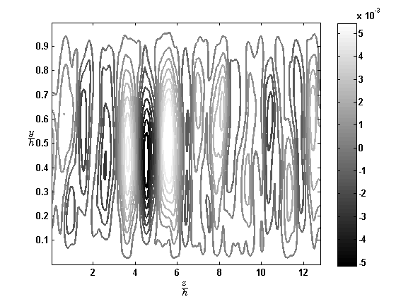
(a) $\psi_{x_{ave}}$ Estimated from $w^{\prime}_{x_{ave}}$

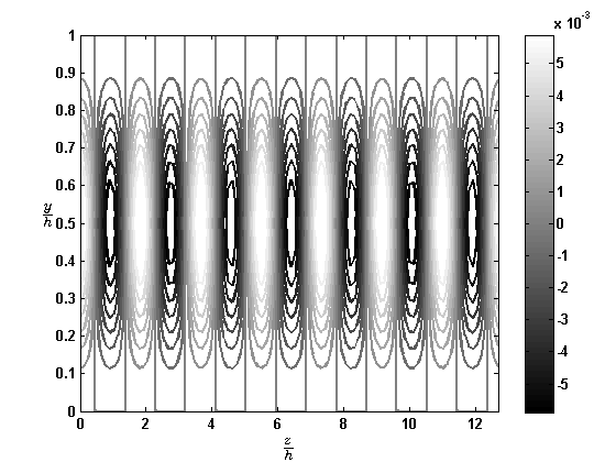
(b) $\psi_{ss}(y,z)=0.0675\sin^{2}\left({\pi y}\right)\cos\left({\frac{{2\pi}}{{1.8}}z}\right)$

Figure 6: (a) Contour plot of the $x$-averaged DNS (as a streamwise constant, $2D/3C$ approximation) spanwise velocity deviations integrated to obtain the stream function, $\psi_{x_{ave}}(y,z)=-\frac{\partial w^{\prime}_{x_{ave}}}{\partial y}$. (b) Contour plot of the simple harmonic model for $\psi_{{ss}}(y,z)=0.00675\sin^{2}\left({\pi y}\right)\cos\left({\frac{{2\pi}}{{1.8}}z}\right)$ with amplitude and wavelengths that approximate DNS data.

The stream function of Equation 5 with the selected $\varepsilon$ and $\lambda_{z}$ was applied to the time-independent form of equation 2, yielding

$$\left(-\frac{\partial\psi_{ss}}{\partial z}\frac{\partial}{\partial y}+\frac{\partial\psi_{ss}}{\partial y}\frac{\partial}{\partial z}+\frac{1}{Re_{w}}\Delta\right)u^{\prime}_{{sw}_{ss}}=\frac{\partial\psi_{ss}}{\partial z}\frac{\partial U}{\partial y}.$$ (6)

A contour plot of the resulting $u^{\prime}_{{sw}_{ss}}(y,z)$ is depicted in Figure 7. This figure shows a $u^{\prime}_{{sw}_{ss}}(y,z)$ with near-wall rolls that are out of spanwise phase with one another similar to those seen in the $x$-averaged DNS data of Figure 5(b). The increased coherence associated with the steady state model relative to the DNS data manifests as an increased variation in the deviation from laminar (amplitude of the surface) particularly at the center of the channel. This effect is emphasized through comparison of the surface plots of Figures 8(a) and 8(b). Note the different vertical axis scales for the two plots.

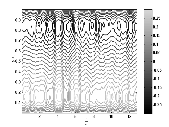
(a) DNS Data

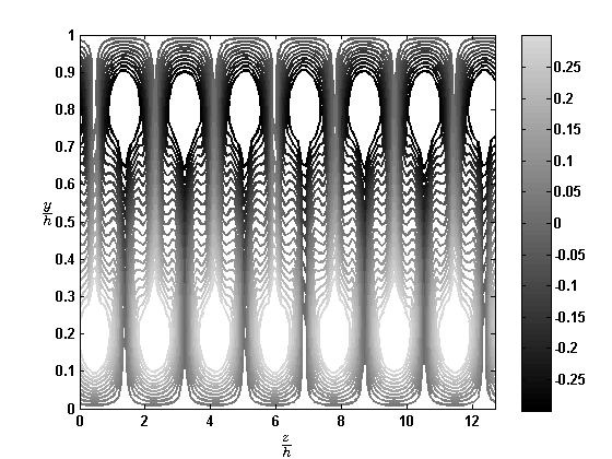
(b) $u^{\prime}_{{sw}_{ss}}$ predicted from $\psi_{ss}$

Figure 7: Contour plots of (a) $x$-averaged DNS data and (b) the $2D/3C$ (streamwise constant) velocity deviations, $u^{\prime}_{{ave}_{ss}}$, obtained using steady state estimate $\psi_{ss}(y,z)=0.00675\sin^{2}\left({\pi y}\right)\cos\left({\frac{{2\pi}}{{1.8143}}z}\right)$, both plotted with the same contour levels.

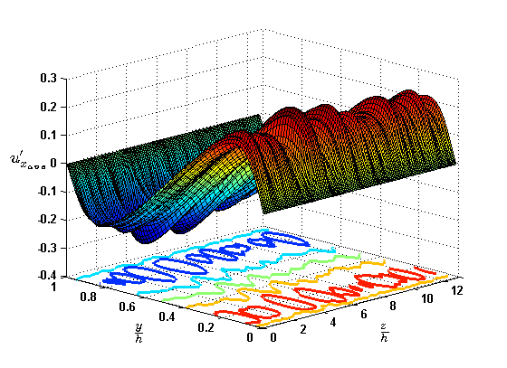
(a) $u^{\prime}_{x_{ave}}$ DNS data

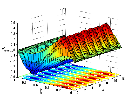
(b) $u^{\prime}_{{sw}_{ss}}$ estimated using $\psi_{ss}(y,z)$

Figure 8: Surface plot of velocity deviations (a) $u^{\prime}_{x_{ave}}(y,z)$ from DNS Data at $Re_{w}=3000$ and (b) $u^{\prime}_{{sw}_{ss}}(y,z)$, obtained using steady state estimate $\psi_{ss}(y,z)=0.00675\sin^{2}\left({\pi y}\right)\cos\left({\frac{{2\pi}}{{1.8143}}z}\right)$ at $Re_{w}=3000$, note the $z$ scale difference between (a) and (b)

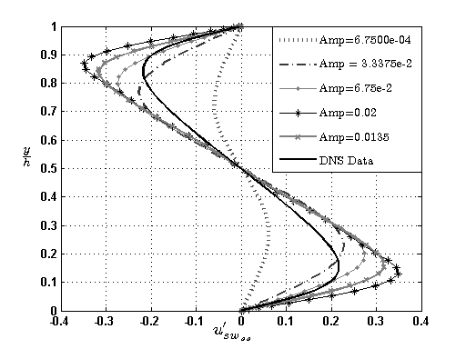
(a) Amplitude Variation

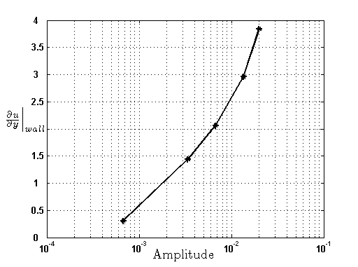
(b) Velocity Gradient at the Wall

Figure 9: (a) Variation of the $2D/3C$ (streamwise constant) velocity deviations, $u^{\prime}_{x_{ave}}$ with $A$; estimates are obtained using steady state estimate $\psi(y,z)=A\sin^{2}\left({\pi y}\right)\cos\left({\frac{{2\pi}}{{1.8143}}z}\right)$ (b) Variation in the velocity gradient at the wall$\left.\frac{\partial u}{\partial y}\right|_{wall}$ with $\psi_{ss}$ amplitude, $A$.

Averages across the span of $u^{\prime}_{sw_{ss}}(y,z)$ for $\varepsilon=0.00675$ as well as for four additional $\varepsilon$ values are compared to a similar average of $u^{\prime}_{x_{ave}}$ from the DNS in Figure 9(a). Clearly using $\psi_{ss}$ from (5) as an input to (6) produces streamwise velocity profiles whose shapes are consistent with $u^{\prime}_{x_{ave}}\approx\overline{u-U}$ from the DNS. The peaks are, however located at different wall-normal positions. An amplitude that exactly matched both the magnitude and location of the DNS peaks was not found even when different values of $k_{z}$ were studied. This is not unexpected because of the simplicity of the wall-normal variation in the steady state model, as well as the streamwise constant and steady state assumptions (clearly the full turbulent field is neither streamwise constant nor time-independent). However, this type of model clarifies the nonlinear role of cross-stream flow features in redistributing energy in the flow field. These results suggest that the phenomenon that is responsible for blunting of the velocity profile in the mean sense is a direct result of the interaction between rolling motions caused by the $y$–$z$ stream function and the laminar profile. In other words, this study provides strong evidence that the nonlinearity needed to generate the turbulent velocity profile comes from the nonlinear terms that are present in the $u^{\prime}_{sw}(y,z,t)$ equation of the $2D/3C$ model (1).

The magnitude of forcing applied to the system is reflected in the amplitude of $\psi_{ss}(y,z)$ which in turn affects the friction Reynolds number, $Re_{\tau}$ through the skin friction arising due to the resultant mean velocity gradient at the wall. Increasing the amplitude ($\varepsilon$) in Equation 5 is analogous to increasing the magnitude of the model uncertainty. These effects are emphasized in Figure 9(b) which provides a plot of $\varepsilon$ versus the velocity gradient at the wall. This behaviour will be discussed in more detail in Section 4.3.

4.3 Time Dependent $2D/3C$ Model

Time-dependent simulations of (2) were carried out using the basic second-order central difference scheme and pseudo-spectral approaches described earlier. Table 2 lists the Reynolds number and forcing amplitude combinations considered. The window used for time averaging was $\Delta t=100000\frac{h}{U_{w}}$.

Figure 10: (a) Contour plot of $\overline{u^{\prime}_{sw}(y,z,t)}$ obtained from the $2D/3C$ model for Case $1$ with the same contour levels as in Figure 7. (b) The surface plot corresponding to (a).

The initial simulation (Case $1$, in Table 2) was carried out at $Re_{w}=\frac{U_{w}h}{\nu}=3000$ with $d_{\psi}(x,y,t)$ drawn from a zero mean Gaussian distribution with standard deviation (noise amplitude) $\sigma_{noise}=0.01$ applied at every point in the mesh.

Table 2: Computation Details

Case	Reynolds Number	$\sigma_{noise}$	$L_{y}\times L_{z}$	$N_{y}\times N_{z}$	Squared Norm of
					the Noise Input
1	$3000$	0.01	$h\times 12.8h$	$75\times 100$	$0.0565$
2	$3000$	0.0125	$h\times 12.8h$	$75\times 100$	$0.0882$
3	$3000$	0.004	$h\times 12.8h$	$75\times 100$	$0.009$
4	$8600$	0.004	$h\times 12.8h$	$75\times 130$	$0.0092$
5	$12800$	0.004	$h\times\sim 16.5h$	$75\times 130$	$0.0092$
6	$12800$	0.001	$h\times\sim 16.5h$	$75\times 130$	$5.77e-04$
Spec 1	$3000$	0.001	$h\times\sim 14.5h$	$40\times 81$	$-$
Spec 2	$3000$	0.002	$h\times\sim 14.5h$	$40\times 81$	$-$

A comparison of Figures 5(b) and 10 shows that contours of constant streamwise velocity deviation from laminar from the DNS and the $2D/3C$ simulation are in good qualitative agreement. In particular, the spanwise offset in spatial phase between peaks from top to bottom is reproduced. While the dominant wavelength from the $2D/3C$ simulation is somewhat longer than the $\lambda_{z}\approx 1.8$ of the DNS (frequency analysis of $\overline{u^{\prime}_{sw}}$ indicates that most of the energy resides in wave lengths between $4\leq\lambda_{z}\leq 6.1$) there is also a significant contribution from $\lambda_{z}\approx 2$. There is noticeably better agreement between the time-dependent model and the DNS (Figure 10 and 8(a)) than for the steady state analysis (Figure 8(b)), likely a consequence of the broadband stochastic, i.e. less coherent and time-dependent, forcing.

4.3.1 Mean Velocity Profile

Averaging the streamwise velocity field obtained for Case $1$ in Table 2 leads to the mean velocity profile (i.e. $\overline{u_{sw}}$) shown in Figure 11(a). The mean profile can also be plotted in inner units (Figure 11(b)) with the use of Equation 3 (with $G=0.1991$ from Tsukahara et al. (2006)) to estimate the friction velocity, $u_{\tau}$. There is good agreement between the DNS and the Case $1$ simulation, even with the assumption of a friction velocity that corresponds to the full flow. However, it is clear that below $y^{+}\approx 20$ the $2D/3C$ model underestimates the expected velocity profile (maximum error $7.4\%$), and above that it overshoots it (maximum error $2.4\%$). There are two obvious first-order interpretations of these discrepancies. First, for cases $1$–$6$, the noise is modeled as being evenly distributed across the grid while in reality the noise is likely higher in the buffer region due to the proximity of the wall, and lower in the overlap layer. An improved noise model might improve the agreement. A second interpretation is that further from the wall the flow is better modeled by the streamwise constant approximation, while streamwise variation is more important in the dynamics of the near-wall region (in agreement with the known variation of the spectral distribution of streamwise energy in the full flow).

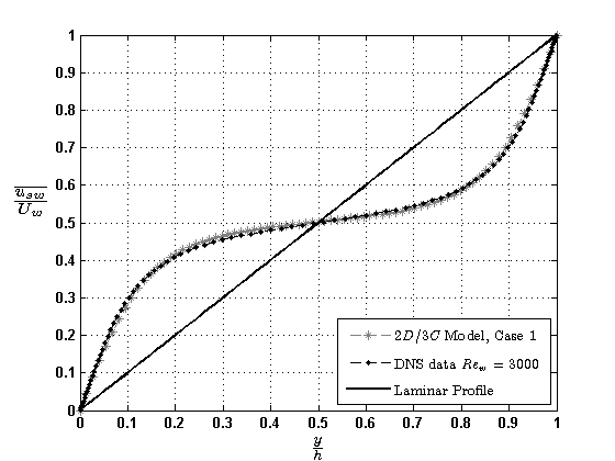
(a) Mean Velocity Profiles

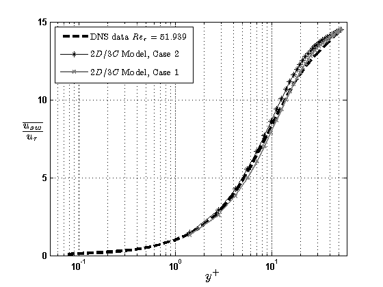
(b) Mean Velocity Inner Units

Figure 11: (a) Comparison of mean velocity profile from the $2D/3C$ model Case $1$, $\overline{u_{sw}(y,z,t)}$, with $\overline{u(x,y,z,t)}$ from DNS. (b) Inner scaled velocity profiles comparison of Cases $1$ and $2$ to the DNS data with $Re_{\tau}\approx 52$ for all data sets.

A second (constant) noise amplitude at the same Reynolds number, Case $2$, is also shown in Figure 11(b). The agreement with the DNS is certainly improved below $y^{+}=20$ (maximum error $6.19\%$ at $y^{+}=19$), but at the expense of larger error further from the wall ($\sim 5-6\%$ between $20<y^{+}<30$). These results further support the idea that a non-uniform noise forcing with increased noise near the wall versus that at channel center may more accurately reflect the conditions in a real flow field. This idea is further explored in Section 4.3.3.

It should be noted that $u_{\tau}$ can also be computed directly from the velocity gradient at the wall. In both cases $Re_{\tau}$ is underestimated by around $10\%$ compared to the estimate from (3). Because of the limited number of points near the wall, the friction relationship from the full flow was preferred, with the understanding that this would only be correct if the 2D/3C model with $\sigma_{noise}$ exactly reproduced the mean flow behavior.

4.3.2 Reynolds Number and Noise Amplitude Trends

Four additional Reynolds number and $\sigma_{noise}$ amplitudes pairs were considered. The details for each of the cases $3$–$6$, along with the computational domain and spatial resolution, are provided in Table 2. Respective values of the norm $\|\cdot\|^{2}$, as computed in Equation (4), of the noise input computed over the box are also reported, since this is a more appropriate measure of the forcing when the box size varies.

It is useful to introduce a normalized version of Equation (1) through the change of variables $\tau=\frac{t}{{Re}}\mbox{ and }\Psi=Re\;\psi$. This creates new expressions for the forcing in (2), $\mathcal{D}_{u}=Re\,d_{u}(=0)$ and $\mathcal{D}_{\Psi}=Re^{2}d_{\psi}$. The expression $\mathcal{D}_{\Psi}=Re^{2}d_{\psi}$ indicates that an increase in noise produces a similar effect to an increase in Reynolds number (actually $\sqrt{Re}$), as observed in the increased deviation from laminar observed with increasing noise amplitude in 9(a). This is especially clear when considering the variation of $Re_{\tau}$ because an increase in noise amplitude directly corresponds to increased velocity gradients at the wall due to the no-slip boundary conditions. Increased profile “blunting” with both increasing $\sigma_{noise}$ (noise input energy) and Reynolds number in cases $2$–$5$ can be observed in figure 12.

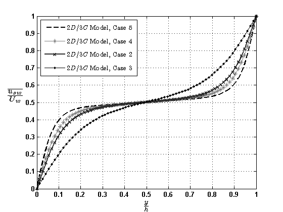
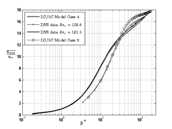
Figure 12: (a) $\overline{u_{sw}(y,z,t)}$ from $2D/3C$ Model for Cases $2-5$ in Table 2 and (b) a comparison of $u^{+}$ versus $y^{+}$ for Cases $4$ and $5$ with $Re_{\tau}$ computed based on the values used in Tsukahara et al. (2006).

For the higher Reynolds numbers (but constant noise amplitude) in Case $4$ and $5$, Figure 12 shows a worsening agreement in inner units with the DNS data from Tsukahara et al. (2006) at $Re_{\tau}=128.5$ and $Re_{\tau}=181.3$, respectively. The underestimation below $y^{+}\approx 30$ (in the buffer layer) is more pronounced, but the agreement above $y^{+}>30$ remains of similar magnitude (max error $\sim 4.94\%$ for $Re_{\tau}=128.5$ and $8.39\%$ for $Re_{\tau}=181.3$). We hypothesize that this worsened agreement may be representative of the increasing scale separation with increased Reynolds number. Near-wall motions that can effectively be modeled as streamwise constant at low Reynolds numbers have an increasingly short streamwise wavelength relative to the motions that scale with outer length scale $\delta$. That the zero-error location consistently occurs around $y^{+}=20$–$30$, commonly thought to be the upper boundary of the buffer layer, is consistent with this scale separation argument. For the same reason, the lack of model resolution in the near-wall region will be exacerbated with increasing $Re_{w}$. In robust control terms, this points once again to an increase in the model uncertainty near the wall versus the channel center. Once again, a better uncertainty model could be accomplished through the use of a ‘structured uncertainty’ which would include an increase in $\sigma_{noise}$ in the near-wall region.

4.3.3 Varying Noise Amplitude and Distribution

A preliminary effort to introduce a non-uniform distribution of noise was carried out by repeating the simulation using a pseudospectral scheme with a Chebyshev interpolant for the wall-normal direction. This scheme naturally produces increased noise near the walls. Cases Spec $1$ and Spec $2$ in Table 2 are two such simulations, both at $Re_{w}=3000$, with $\sigma_{noise}=0.001$ and $\sigma_{noise}=0.002$ respectively. Figure 13 shows the resulting mean velocity profiles. Clearly the noise level is too low for Spec $1$, however for Spec $2$ the maximum error occurs in the buffer layer and is of the order $5$–$6\%$. The results of the spectral simulations indicate that by further noise shaping one could improve the agreement throughout the profile and across a range of Reynolds numbers.

As previously discussed there is a strong relationship between the friction Reynolds number and $\sigma_{noise}$. As an illustration of this, Figure 13 shows that one can obtain similar mean velocity profiles at two different Reynolds numbers simply by adjusting the noise amplitude, i.e. a higher Reynolds number requires a smaller (uniform) noise amplitude to develop a mean velocity profile that is similar to that of a lower Reynolds number case with higher noise amplitude. This result is consistent with observations of higher transitional Reynolds number associated with “quiet” experiments compared to ones with high background disturbance levels. Alternatively, a fixed amplitude noise produces a larger response (more blunting) at higher $Re$ than lower ones because disturbance amplification increases with increasing Reynolds number. This example makes it clear that the noise amplitude and the friction Reynolds number are tightly coupled, while giving further evidence that Reynolds number dependent wall-normal shaping of the noise would be required to get a better model representation of the turbulent mean velocity profiles.

4.3.4 Characterization of the (small) disturbance amplification

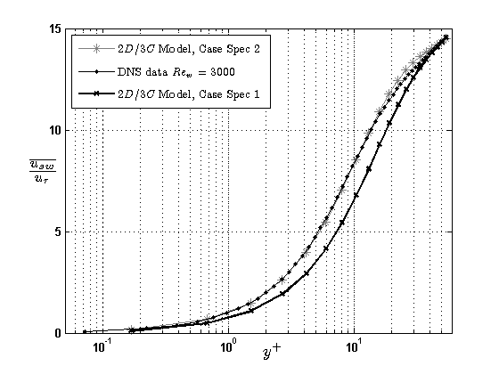
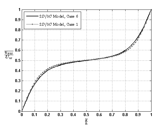
Figure 13: (a) Comparison of $u^{+}$ versus $y^{+}$ from $2D/3C$ Model using Chebyshev spacing in $y$ with DNS data at $Re_{w}=3000$ based on $G=0.1991$ ($Re_{\tau}\approx=52$) (b) Comparison of $\overline{u_{sw}(y,z,t)}$ from $2D/3C$ Model at for Case $1$ ($Re_{w}=3000$ with $\sigma_{noise}=0.01$, $energy=0.0882$), and Case $6$ ($Re_{w}=12800$ with $\sigma_{noise}=0.001$, $energy=5.77e-04$) same grid and box size.

The results described herein indicate that a very small amount of stochastic noise forcing limited to the cross-stream components produces a very large response which corresponds to a behaviour that is not a solution of the unforced equations. The ability of our model (Equation 1), which has a unique solution in the unforced case, to produce a new flow condition due to such a forcing supports the notion that the model is not robust to small disturbances/uncertainty. The potential for disturbance amplification is not new, in fact it comes directly from the features of the LNS previously discussed, however the creation and maintenance of the new flow state is different and cannot come through the use of a linear model. A simple characterization of the amplification maintained through the forced response of (2), or the lack of robustness (‘fragility’) of the system, can be formulated as follows.

Defining the squared $2$-norm of the streamwise component of (2) (i.e. $\|\overline{u^{\prime}_{sw}}\|^{2}$) to be the increase in streamwise energy from the base (laminar) flow, a so-called amplification factor is given by,

$$\Gamma_{u}=\frac{\|\overline{u^{\prime}_{sw}}\|^{2}}{\|\sigma_{noise}\|^{2}}$$ (7)

which is a measure of the output energy for a given input (noise forcing amplitude). $\Gamma_{u}$ is a nonlinear analog of the ‘ensemble energy density’ described in previous studies of the input-output response of the LNS, e.g. (Bamieh & Dahleh, 2001; Jovanović & Bamieh, 2005). Those investigations showed that the coupling between the Orr-Sommerfeld and Squire modes enables very large, Reynolds number dependent disturbance amplification. The amplification factor for case $3$–$5$, which all have approximately the same input energy, are respectively $\Gamma_{u}\approx 680$, $\Gamma_{u}\approx 2200$, and $\Gamma_{u}\approx 2920$. These trends are consistent with the low Reynolds number scaling trends based on the OSS equations. This agreement reflects the effective restriction of the streamwise constant assumption to amplification of the $k_{x}=0$ modes (most amplified in the linear equation) as well as the source of the amplification in the $2D/3C$ model: a coupling in a similar linear operator, given by

$$\frac{\partial}{\partial t}\left[\begin{array}[]{c}\psi\\ u_{sw}^{\prime}\end{array}\right]=\left[\begin{array}[]{cc}\Delta^{-1}\left(\frac{1}{Re_{w}}\Delta\Delta\right)&0\\ -\frac{\partial U}{\partial y}\frac{\partial}{\partial z}&\frac{1}{Re_{w}}\Delta\end{array}\right]\left[\begin{array}[]{c}\psi\\ u_{sw}^{\prime}\end{array}\right].$$ (8)

In this way computing $\Gamma_{u}$ from the simulation of (2) is analogous to studying the steady state nonlinear response to the most amplified $3D$ mode, (i.e. the $k_{x}=0$ mode).

Equivalent amplification relationships between the cross-stream velocity components and $\sigma_{noise}$ could similarly be investigated.

Structures with long streamwise coherence have long been shown to have a significant role in both transition and fully developed turbulent flows. Based on these observations we study a streamwise constant projection of the Navier-Stokes equations for plane Couette flow, the $2D/3C$ model. Simulation of this model under small amplitude Gaussian forcing captures the turbulent mean velocity profile at low Reynolds numbers. Appropriate Reynolds number trends are also reproduced.

A weakly nonlinear, steady state analysis demonstrates that $2D$ stream functions can produce appropriate mean velocity distributions when they are nonlinearly coupled to the $2D/3C$ streamwise velocity. This indicates that ‘swirling motions’ in the $y$–$z$ plane produce features consistent with the mean characteristics of fully developed turbulence. It also provides evidence that the nonlinear coupling in the $2D/3C$ model is responsible for creating the well known characteristic ‘S’ shaped turbulent velocity profile.

The use of small amplitude stochastic forcing as an input to the $2D/3C$ (nominal) model is based on ideas from robust control. Experimental observations are used to simplify the NS equations to form this nominal model and the noise forcing is used to capture both uncertain parameter values and unmodeled effects. The resulting forced $2D/3C$ model allows one to isolate phenomena that can not be decoupled from a full simulation of NS while maintaining a sufficiently rich description of the physics that govern turbulent flow. Our physics-based model should provide greater insight into the dynamics of the system than an empirical technique. Such a model may also allow better control design.

The linearized $2D/3C$ model (8) maintains the properties responsible for large disturbance amplification which have also been linked to subcritical transition. Maintenance of these linear mechanisms is critical to the success of this approach. It is the combination of these linear processes along with the momentum transfer from the two nonlinear terms in the streamwise velocity equation that enable the model to capture the blunted turbulent velocity profile. This line of inquiry provides a complementary perspective to transient growth and structurally based models, in that the $2D/3C$ model offers some improvement in analytic tractability at the expense of streamwise detail. The results are especially promising because the computational and analytical tractability of this model makes it well suited to higher Reynolds number studies.

A natural extension of the present work would be the development of a more appropriate model for the noise distribution. It is common in the controls literature for a system to have a so-called structured uncertainty which is based on the physics of a particular system. In this work the limitation of noise to only the $\Delta\psi$ equation represents a first level of such an approach. Knowledge of the physics, for example that the near-wall region is under-resolved in the $2D/3C$ model, is a first step. Numerical or experimental studies aimed at characterizing true spatial noise forcing patterns would further help in determining the correct model for noise distribution.

5 Acknowledgements

The authors would like to thank H. Kawamura and T. Tsukahara for providing us with their DNS data. This research is sponsored in part through a grant from the Boeing Corporation. B.J.M. gratefully acknowledges support from NSF-CAREER award number 0747672 (program managers W. W. Schultz and H. H. Winter).

References

- del Álamo & Jiménez (2006) del Álamo, J. C. & Jiménez, J. 2006 Linear energy amplification in turbulent channels. J. Fluid Mech. 559, 205–213.
- Bamieh & Dahleh (2001) Bamieh, B. & Dahleh, M. 2001 Energy amplification in channel flows with stochastic excitation. Phys. of Fluids 13 (11), 3258–3269.
- Barkley & Tuckerman (2007) Barkley, D. & Tuckerman, L. S. 2007 Mean flow of turbulent-laminar patterns in plane Couette flow. J. Fluid Mech. 576, 109–137.
- Bech et al. (1995) Bech, K. H., Tillmark, N., Alfredsson, P. H. & Andersson, H. I. 1995 An investigation of turbulent plane Couette flow at low Reynolds numbers. J. Fluid Mech. 286, 291–325.
- Bobba (2004) Bobba, K. M. 2004 Robust flow stability: Theory, computations and experiments in near wall turbulence. PhD thesis, California Institute of Technology, Pasadena, CA, USA.
- Bobba et al. (2002) Bobba, K. M., Bamieh, B. & Doyle, J. C. 2002 Highly optimized transitions to turbulence. In Proc. of IEEE Conf. on Decision and Control, pp. 4559–4562. Las Vegas, NV, USA.
- Butler & Farrell (1992) Butler, K. M. & Farrell, B. F. 1992 Three-dimensional optimal perturbations in viscous shear flow. Phys. of Fluids A 4, 1637–1650.
- Butler & Farrell (1993) Butler, K. M. & Farrell, B. F. 1993 Optimal perturbations and streak spacing in wall-bounded turbulent shear flow. Phys. of Fluids A 5, 774–777.
- Chung & McKeon (2010) Chung, D. & McKeon, B. J. 2010 Large-eddy simulation investigation of large-scale structures in a long channel flow. J. Fluid Mech. 661, 341 – 364.
- Doyle et al. (1991) Doyle, J. C., Francis, B. & Tannenbaum, A. 1991 Feedback Control Theory. New York: MacMillan Company.
- El Telbany & Reynolds (1982) El Telbany, M. M. M. & Reynolds, A. J. 1982 The structure of turbulent plane Couette flow. Trans. ASME: J. of Fluids Engineering 104, 367–372.
- Farrell (1988) Farrell, B. F. 1988 Optimal excitation of perturbations in viscous shear flow. Phys. of Fluids 31 (8), 2093–2102.
- Farrell & Ioannou (1993a) Farrell, B. F. & Ioannou, P. J. 1993a Optimal excitation of three-dimensiogal perturbations in viscous constant shear flow. Phys. of Fluids A 5 (6), 1390–1400.
- Farrell & Ioannou (1993b) Farrell, B. F. & Ioannou, P. J. 1993b Stochastic forcing of the linearized Navier-Stokes equations. Phys. of Fluids A 5 (11), 2600–2609.
- Farrell & Ioannou (1998) Farrell, B. F. & Ioannou, P. J. 1998 Perturbation structure and spectra in turbulent channel flow. Theoretical and Computational Fluid Dynamics 11, 237–250.
- Gayme et al. (2009) Gayme, D. F., McKeon, B., Papachristodoulou, A. & Doyle, J. C. 2009 model of large scale structures in turbulence in plane Couette flow. In Proc. of Int’l Symposium on Turbulence and Shear Flow Phenomenon. Seoul, Korea.
- Gibson et al. (2009) Gibson, J. F., Halcrow, J. & Cvitanović, P. 2009 Equilibrium and travelling-wave solutions of plane Couette flow. J. Fluid Mech. 638, 243–266.
- Guala et al. (2006) Guala, M., Hommema, S. E. & Adrian, R. J. 2006 Large-scale and very-large-scale motions in turbulent pipe flow. J. Fluid Mech. 554, 521–542.
- Gustavsson (1991) Gustavsson, L. H. 1991 Energy growth of three-dimensional disturbances in plane Poiseuille flow. J. Fluid Mech. 224, 241–260.
- Hamilton et al. (1995) Hamilton, J. M., Kim, J. & Waleffe, F. 1995 Regeneration mechanisms of near-wall turbulence structures. J. Fluid Mech. 287, 317–348.
- Henningson & Reddy (1994) Henningson, D. S. & Reddy, S. C. 1994 On the role of linear mechanisms in transition to turbulence. Phys. of Fluids 6 (3), 1396–1398.
- Hutchins & Marusic (2007a) Hutchins, N. & Marusic, I. 2007a Evidence of very long meandering structures in the logarithmic region of turbulent boundary layers. J. Fluid Mech. 579, 1–28.
- Hutchins & Marusic (2007b) Hutchins, N. & Marusic, I. 2007b Large-scale influences in near-wall turbulence. Phil. Trans. Royal Society London A 365, 647–664.
- Jiménez & Pinelli (1999) Jiménez, J. & Pinelli, A. 1999 The autonomous cycle of near-wall turbulence. J. Fluid Mech. 389, 335–359.
- Jovanović & Bamieh (2001) Jovanović, M. R. & Bamieh, B. 2001 The spatio-temporal impulse response of the linearized Navier-Stokes equations. In Proc. of the 2001 American Control Conf., pp. 1948–1953. Arlington, VA, USA.
- Jovanović & Bamieh (2004) Jovanović, M. R. & Bamieh, B. 2004 Unstable modes versus non-normal modes in supercritical channel flows. In Proc. of the 2004 American Control Conf., pp. 2245–2250. Boston, MA, USA.
- Jovanović & Bamieh (2005) Jovanović, M. R. & Bamieh, B. 2005 Componentwise energy amplification in channel flows. J. Fluid Mech. 534, 145–183.
- Kim & Lim (2000) Kim, J. & Lim, J. 2000 A linear process in wall-bounded turbulent shear flows. Phys. of Fluids Letters 12 (8), 1885–1888.
- Kim & Adrian (1999) Kim, K. J. & Adrian, R. J 1999 Very large scale motion in the outer layer. Phys. of Fluids 11 (2), 417–422.
- Kitoh et al. (2005) Kitoh, O., Nakabyashi, K. & Nishimura, F. 2005 Study on mean velocity and turbulence characteristics of plane Couette flow: Low-Reynolds-number effects and large longitudinal vortical structure. J. Fluid Mech. 539, 199–227.
- Kitoh & Umeki (2008) Kitoh, O. & Umeki, M. 2008 Experimental study on large-scale streak structure in the core region of turbulent plane Couette flow. Phys. of Fluids 20 (2), 025107–025111.
- Kline et al. (1967) Kline, S. J., Reynolds, W. C., Schraub, F. A. & Runstadler, P. W. 1967 The structure of turbulent boundary layers. J. Fluid Mech. 30, 741–773.
- Komminaho et al. (1996) Komminaho, J., Lundbladh, A. & Johansson, A. V. 1996 Very large structures in plane turbulent Couette flow. J. Fluid Mech. 320, 259–285.
- Lee & Kim (1991) Lee, M. J. & Kim, J. 1991 The structure of turbulence in a simulated plane Couette flow. Thin Solid Films 1, 531–536.
- Lumley (1967) Lumley, J. L. 1967 The structure of inhomogeneous turbulence. In Atmospheric Turbulence and Wave Propagation (ed. A. M.Yaglom & V. I. Tatarski), pp. 166–178. Moscow: Nauka.
- Luo (2006) Luo, W. 2006 Wiener chaos expansion and numerical solutions of stochastic partial differential equations. PhD thesis, California Institute of Technology, Pasadena, CA, USA.
- Mathis et al. (2009) Mathis, R., Hutchins, N. & Marusic, I. 2009 Large-scale amplitude modulation of the small-scale structures of turbulent boundary layers. J. Fluid Mech. 628, 311–337.
- Morinishi (1995) Morinishi, Y. 1995 Conservative properties of finite difference schemes for incompressible flow. In Center for Turbulence Research Annual Research Briefs, pp. 121 –132. Stanford University/NASA Ames.
- Morrison et al. (2004) Morrison, J. F., McKeon, B. J., Jiang, W. & Smits, A. J. 2004 Scaling of the streamwise velocity component in turbulent pipe flow. J. Fluid Mech. 1508, 99–131.
- Nagata (1990) Nagata, M. 1990 Three-dimensional finite-amplitude solutions in plane Couette flow: bifurcation from infinity. J. Fluid Mech. 217, 519–527.
- Orlandi & Jiménez (1994) Orlandi, P. & Jiménez, J. 1994 On the generation of turbulent wall friction. Phys. of Fluids 16 (2), 634–641.
- Reddy & Ioannou (2000) Reddy, S.C. & Ioannou, P.J. 2000 Laminar-Turbulent Transition IUTAM 99, chap. Energy Transfer Analysis of Turbulent Plane Couette Flow, pp. 211–216. Berlin: Springer-Verlag.
- Reddy & Henningson (1993) Reddy, S. C. & Henningson, D. S. 1993 Energy growth in viscous channel flows. J. Fluid Mech. 252, 209–238.
- Robertson (1959) Robertson, J. M. 1959 On turbulent plane Couette flow. In Proc. of the Midwestern Conf. on Fluid Mech., pp. 169 –182.
- Robertson & Johnson (1970) Robertson, J. M. & Johnson, H. F. 1970 Turbulence structure in plane Couette flow. J. Engineering Mech. Division 96, 1171–1181.
- Schoppa & Hussain (2002) Schoppa, W. & Hussain, F. 2002 Coherent structure generation in near-wall turbulence. J. Fluid Mech. 453, 57–108.
- Smith et al. (2005) Smith, T. R., Moehlis, J. & Holmes, P. 2005 Low-dimensional modelling of turbulence using the proper orthogonal decomposition: A tutorial. Nonlinear Dynamics 41, 275–307.
- Swanson (2007) Swanson, J. 2007 Variations of the solution to a stochastic heat equation. Annals of Probability 35, 2122–2159.
- Tillmark (1995) Tillmark, N. 1995 Experiments on transition and turbulence in plane Couette flow. PhD thesis, Royal Institute of Technology, Stockholm, Sweden.
- Tillmark & Alfredsson (1998) Tillmark, N. & Alfredsson, P. H. 1998 Large scale structure in turbulent plane Couette flow. In Advances in Turbulence VII (ed. U. Frish), pp. 59–62. Saint-Jean Cap Ferrat, France: Kluwer, Dordrecht.
- Trefethen et al. (1993) Trefethen, L. N., Trefethen, A. E., Reddy, S. C. & Driscoll, T. A. 1993 Hydrodynamic stability without eigenvalues. Science 261 (5121), 578–584.
- Tsukahara et al. (2006) Tsukahara, T., Kawamura, H. & Shingai, K. 2006 DNS of turbulent Couette flow with emphasis on the large-scale structure in the core region. J. Turbulence 7 (019).
- Tullis & Pollard (1993) Tullis, S. & Pollard, A. 1993 Modeling the time-dependent flow over riblets in the viscous wall region. Applied Scientific Research 50 (3-4), 299–314.
- Waleffe (1990) Waleffe, F. 1990 Proposal for a self-sustaining mechanism in shear flows. Tech. Rep.. Center for Turbulence Research, Stanford University/NASA Ames.
- Waleffe (1997) Waleffe, F. 1997 On a self-sustaining process in shear flows. Phys. Fluids 9 (4), 883–900.
- Waleffe et al. (1991) Waleffe, F., Kim, J. & Hamilton, J. 1991 On the origin of streaks in turbulent shear flows. In Eighth Int’l Symposium on Turbulent Shear Flows. Munich, Germany.
- Weideman & Reddy (2000) Weideman, J. A. C. & Reddy, S. C. 2000 A MATLAB differentiation matrix suite. ACM Transactions on Mathematical Software 26 (4), 465–519.
- Zhou et al. (1996) Zhou, K., Doyle, J. C. & Glover, K. 1996 Robust and Optimal Control. Upper Saddle River, NJ: Prentice Hall.