Submillimeter Variability and the Gamma-ray Connection in Fermi Blazars

Abstract

We present multi-epoch observations from the Submillimeter Array (SMA) for a sample of 171 bright blazars, 43 of which were detected by Fermi during the first three months of observations. We explore the correlation between their gamma-ray properties and submillimeter observations of their parsec-scale jets, with a special emphasis on spectral index in both bands and the variability of the synchrotron component. Subclass is determined using a combination of Fermi designation and the Candidate Gamma-Ray Blazar Survey (CGRaBS), resulting in 35 BL Lac objects and 136 flat-spectrum radio quasars (FSRQs) in our total sample. We calculate submillimeter energy spectral indices using contemporaneous observations in the 1 mm and 850 micron bands during the months August–October 2008. The submillimeter light curves are modeled as first-order continuous autoregressive processes, from which we derive characteristic timescales. Our blazar sample exhibits no differences in submillimeter variability amplitude or characteristic timescale as a function of subclass or luminosity. All of the the light curves are consistent with being produced by a single process that accounts for both low and high states, and there is additional evidence that objects may be transitioning between blazar class during flaring epochs.

I INTRODUCTION

The timescales on which high-amplitude flaring events occur in blazars indicate that much of the energy is being produced deep within the jet on small, sub-parsec scales (sikora01AIPCS, ; sikora01ASPCS, ). Understanding if/how emission differs between blazar subclasses (i.e., BL Lacs objects and flat-spectrum radio quasars (FSRQs)) may offer important insight into the similarity between blazars and, furthermore, can provide constraints on the formation and acceleration of the jets themselves.

For the synchrotron component of blazar spectra, the low-frequency spectral break due to synchrotron self-absorption moves to higher frequencies as one measures closer to the base of the jet (sikora01ASPCS, ). This often places the peak of the spectrum in the millimeter and submillimeter bands, where the emission is optically-thin and originates on parsec and sub-parsec scales (stevens94, ), allowing direct observation of the most compact regions near the central engine. The high energy $\gamma$-ray emission originates as a Compton process, typically a combination of synchrotron-self-Compton (SSC) and external-radiation-Compton (ERC). Depending on the source properties, the synchrotron photons or external photons are upscattered by the same population of electrons that emit the millimeter and submillimeter spectra. Therefore the submillimeter and $\gamma$-ray emission are closely linked and give the full information about the source emission.

A systematic study of the submillimeter properties of the entire sample of Fermi blazars has yet to be conducted and is one of the primary goals of our work. We present here preliminary analysis of the submillimeter properties of Fermi blazars detected by the Submillimeter Array (SMA) at 1mm and 850$\mu$m, including an investigation of variable behavior and the determination of submillimeter energy spectral indices. In addition, we consider the connection to the observed $\gamma$-ray indices and luminosities.

II SMA BLAZARS

The Submillimeter Array (ho04, ) consists of eight 6 m antennas located near the summit of Mauna Kea. The SMA is used in a variety of baseline configurations and typically operates in the 1mm and 850$\mu$m windows, achieving spatial resolution as fine as 0.25” at 850$\mu$m. The sources used as phase calibrators for the array are compiled in a database known as the SMA Calibrator List (gurwell07, ). Essentially a collection of bright objects (stronger than 750 mJy at 230 GHz and 1 Jy at 345 GHz), these sources are monitored regularly, both during science observations and dedicated observing tracks.

To select our sample, we identified objects in the calibrator list that were also classified as BL Lacs or FSRQs by the Candidate Gamma-Ray Blazar Survey (healey08, , CGRaBS). Of the 243 total objects in the calibrator list, 171 (35 BL Lacs and 136 FSRQs) have positive blazar class identifications, although there are three sources (J0238+166, J0428-379, and J1751+096) which have conflicting classifications between Fermi and CGRaBS. Some blazars found in the calibrator list have been studied extensively (e.g., 3C 279 and 3C 454.3) but the SMA blazars have not been studied collectively.

Forty-four of the objects in our total blazar sample were detected by Fermi and can be found in the catalog of LAT Bright AGN Sources (LBAS) from Abdo et al. abdo09 . J0050-094 has no redshift in either the LBAS catalog or CGRaBS and is not included in our study. Of the 43 remaining sources, 14 are BL Lac objects and 29 are FSRQs, with $0.03\leq z\leq 2.19$.

We examined submillimeter light curves for all of the SMA blazars, with observations beginning in approximately 2003 (see Figure 1). Typically, the 1mm band is much more well-sampled in comparison to the 850 m band, but visual inspection reveals that the regularity and quality of observations vary greatly from source to source. Many of the objects exhibit nonperiodic variability, either in the form of persistent, low-amplitude fluctuations or higher amplitude flaring behavior.

Figure 1: The SMA light curves for 3C 454.3. The open circles represent the 850$\mu$m observations, and the open triangles represent the 1mm observations.

II.1 Submillimeter Properties

Submillimeter Luminosities. Since we are primarily concerned with comparisons to Fermi observations, we note that only 129 of the SMA blazars (23 BL Lacs and 106 FSRQs) were observed by the SMA in either band during the three months August-October 2008. For these objects, submillimeter luminosities are calculated in the standard way:

$$\nu_{e}L_{\nu_{e}}=4\pi D_{\rm L}^{2}{\nu_{\rm{obs}}F_{\rm{obs}}\over 1+z},$$ (1)

where $D_{\rm L}$ is the luminosity distance, $\nu_{\rm obs}$ is the frequency of the observed band, and $F_{\rm obs}$ is the average flux (in erg cm^-2 s^-1 Hz^-1) over the three month period. We adopt a lambda cold dark matter cosmology with values of $H_{0}=71$ km s^-1 Mpc^-1, $\Omega_{\mathrm{M}}=0.27$, and $\Lambda=0.73$.

Energy Spectral Indices. We derive submillimeter spectral energy indices from observations quasi-simultaneous with the Fermi observations. To be consistent with the use of $\alpha_{\gamma}$, we define spectral energy index as $\nu F_{\nu}=\nu^{-\alpha_{\mathrm{S}}}$ and calculate $\alpha_{\mathrm{S}}$ from the average of the energy spectral indices over the corresponding three months. We only calculate $\alpha_{\rm S}$ for the 16 objects (8 BL Lacs and 35 FSRQs) with observations at both 1mm and 850$\mu$m during this time frame.

III VARIABILITY ANALYSIS

III.1 Variability Index

Figure 2: Variability index for our sample (top: 1mm, bottom: 850$\mu$m), with FSRQs as the hatched distribution and BL Lacs as the solid distribution. There is no signi cant difference in the class distributions in either band; the “tail” to the left is populated by objects with errors larger than the intrinsic variability.

We roughly characterize the level of variability of each source using the variability index from Hovatta et al. hovatta08 :

$$V\,=\,\frac{(F_{\mathrm{max}}-\sigma_{F_{\mathrm{max}}})-(F_{\mathrm{min}}+\sigma_{F_{\mathrm{min}}})}{(F_{\mathrm{max}}-\sigma_{F_{\mathrm{max}}})+(F_{\mathrm{min}}+\sigma_{F_{\mathrm{min}}})}$$ (2)

Figure 2 shows the distribution for the SMA blazars. Objects with $V\leq 0$ are typically unsuitable for more detailed variability analysis for one of two reasons: (1) too few data points or (2) flux measurement uncertainties on the order of the amplitude of observed variability. It is important to note that, due to discrepancies between the sampling frequency in both bands, the variability indices for the 850$\mu$m band may be artificially depressed due to the fact that there are not always corresponding measurements at higher frequencies during flaring epochs.

III.2 First-Order Continuous Autoregression

We follow the method of Kelly et al. kelly09 , who model quasar optical light curves as a continuous time first-order autoregressive process (CAR(1)) in order to extract characteristic time scales and the amplitude of flux variations. Although flaring behavior is not typically thought of as an autoregressive process, we find that the light curves are well-fit by the models and therefore adopt the method here to study blazar submillimeter light curves.

The CAR(1) process is described by a stochastic differential equation (kelly09, ),

$$dS(t)\,=\,\frac{1}{\tau}S(t)\,dt+\sigma\sqrt{dt}\,\epsilon\,(t)+b\,dt,$$ (3)

associated with a power spectrum of the form

$$P_{X}(f)\,=\,\frac{2\sigma^{2}\tau^{2}}{1+(2\pi\tau f)^{2}}.$$ (4)

In equations 3 and 4, $\tau$ is called the “relaxation time” of the process $S(t)$ and is identified by the break in $P_{X}(f)$. The power spectrum appears flat for timescales longer than this and falls off as $1/f^{2}$ for timescales shorter than the characteristic timescale of the process.

Taking the logarithm of the blazar light curve (in Jy) to be $S(t)$, we adopt $\tau$ (in days) as the characteristic timescale of variability, after which the physical process “forgets” about what has happened at time lags of greater than $\tau$. The two other relevant parameters, $\sigma$ and $\mu=b/a$, are the overall amplitude of variability and the logarithm of mean value of the light curve, respectively.

In the routine, we construct an autoregressive model for the light curves for a minimum of 100,000 iterations and calculate the value of $\tau$ from the break in the power spectrum in each instance. Due to the limited number of observations in the 850$\mu$m band, we performed this autoregressive analysis only for the 1mm light curves, which typically have more than 10 points per light curve.

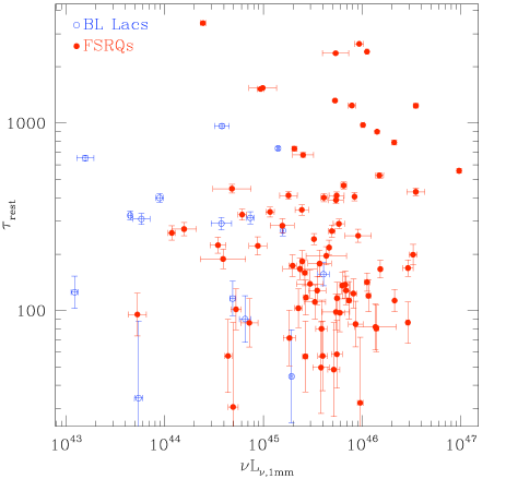
Figure 3: Characteristic timescale (days) versus submillimeter luminosity (erg s^-1) in the 1mm band for all objects. Physically, $\tau$ represents a “relaxation timescale”, the timescale beyond which events are no longer correlated.

This method yielded some surprising results. In Figure 3, we see that the BL Lacs and FSRQs exhibit virtually no difference in characteristic timescale, with both classes extending across a large range in $\tau$. Because of the uncertainty for objects with shorter characteristic timescales, it is hard to draw any definitive conclusions about the differences between classes. It is important to note that $\tau$ does not necessarily represent a flaring timescale, which is a behavior that typically operates on a scale of $\sim$10–100 days and not on the longer timescales we see in $\tau$.

IV CONNECTION WITH GAMMA-RAYS

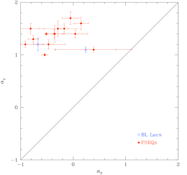
Figure 4: The $\gamma$-ray index versus submillimeter index plane. The blazars fall more steeply in the $\gamma$-rays than in the submillimeter band, where most are, in fact, rising. This LAT-detected sample contrasts with the full SMA sample, where the blazars are more distributed around $\alpha_{\rm S}\sim$ 0.

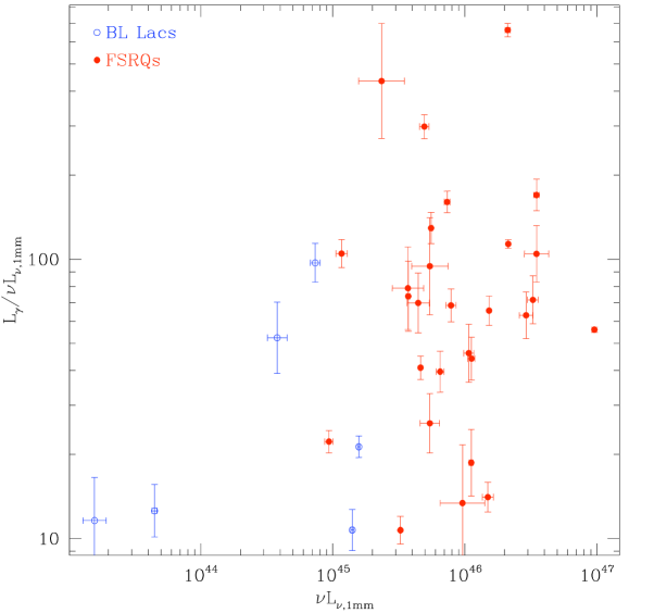
Figure 5: Ratio of $\gamma$-ray luminosity to submillimeter luminosity in the 1mm band. The location of an object in this plot should be directly correlated with its blazar “state”, with FSRQs occupying the upper right and BL Lacs the lower left. Flat-spectrum radio quasar 3C 454.3 is the object with the highest submillimeter luminosity in this plot.

In general, we find that in the submillimeter, we are observing these blazars at or near the peak of the synchrotron component ($\alpha_{\rm S}\sim 0$), but that Fermi-detected sources have more negative energy spectral indices overall than Fermi-nondetected sources. In Figure 4, we see that while the majority of Fermi blazars are observed on the rising part of the synchrotron component (at lower energies than the peak), all of the objects have very steeply falling $\gamma$-ray energy spectral indexes, putting the $\gamma$-ray peak at lower energies than the observed Fermi band. Knowing that we are not observing the synchrotron and $\gamma$-ray components at analagous points in the spectrum may allow us to better understand the magnetic field in the parsec-scale jet region and the population of external photons that is being upscattered to $\gamma$-rays.

In Figure 5, the ratio between $L_{\gamma}$ and $\nu L_{\nu\rm,1mm}$ reflects the division between BL Lacs and FSRQs as well as the presence of SSC versus ERC. Here, we use submillimeter luminosity as a proxy for jet power, which is correlated with the integrated luminosity of the synchrotron component. Elevated $\gamma$-ray luminosity with respect to the synchrotron component (which is often seen in FSRQs) suggests the upscattering of external photons off the synchrotron-emitting electrons. These objects should occupy the upper right of the ratio/jet power plot, and BL Lacs, which generally exhibit components with roughly comparable luminosities, should occupy the lower left. It is clear from the figure, however, that many FSRQs exhibit ratios similar to those of the BL Lacs and vis versa.

Sikora et al. sikora08 report that, during its flaring epochs, 3C 454.3 transitions from its typical FSRQ state to a more BL Lac-like state, where the synchrotron component emits much more strongly compared to the $\gamma$-ray component than during its “low state”. 3C 454.3, which is the highest submillimeter luminosity FSRQ in our sample, would then shift down and to the right in Figure 5 when it enters a flaring period. For the first three months of the Fermi mission, 3C 454.3 was not flaring, which may explain its present location in Figure 5. The three objects for which there is a type discrepancy between CGRaBS and LBAS are all FSRQs (in CGRaBS) and exhibit low luminosity ratios and high luminosity, which suggest they may be undergoing the same changes as 3C 454.3. A possible interpretation of the elevated luminosity ratios observed in some BL Lacs objects is that there has been a dramatic increase in $\gamma$-ray luminosity due to ERC, which would not be reflected in the synchrotron component.

V CONCLUSIONS

The motivation for observing blazars in the submillimeter is to study behavior close to the central engine, where the jet material is presumably still being accelerated. The separate emission processes that contribute to overall SED may present differently in BL Lacs and FSRQs, allowing us to understand the similarities and differences between blazar types. We have investigated these differences between objects in terms of submillimeter behavior and, in conclusion, find that

• The SMA blazars exhibit submillimeter energy spectral indexes that follow the spectral sequence interpretation of blazars.

• BL Lacs and FSRQs do not exhibit significant differences in amplitude of submillimeter variability or characteristic timescale, but our sample of BL Lacs may be dominated by high-peaked BL Lacs (HBLs), which exhibit observational similarities with FSRQs.

• Blazar submillimeter light curves are consistent with being produced by a single process that accounts for both high and low states, with characteristic timescales 10 $<\tau_{\rm rest}<$ 500 days.

• The blazars detected by Fermi have synchrotron peaks at higher frequencies, regardless of submillimeter luminosity.

• FSRQs exhibit higher ratios of $\gamma$-ray to submillimeter luminosity than BL Lacs (Figure 5), but all objects inhabit a region of parameter space suggesting transitions between states during flaring epochs.

As Fermi continues to observe fainter sources, the sample of objects for which we can perform this type of analysis will increase and provide better limits on our results. To understand the physical relevance of these results, however, it is important to be able to distinguish between the difference in variability between BL Lacs and FSRQs. One avenue for exploring this difference is to monitor changing submillimeter energy spectral index and the ratio of $\gamma$-ray to submillimeter luminosity as functions of time. The full meaning of the results of our autoregressive method is not yet clear, and will require better-sampled blazar light curves and the comparison between $\tau_{\rm rest}$ with physical timescales such as the synchrotron cooling timescale. These analyses would allow us to place constraints on the processes occurring near the base of the jet in blazars and further understand the intimate connection between them.

- (1) M. Sikora and G. Madejski, in American Institute of Physics Conference Series, edited by F. A. Aharonian and H. J. Völk (2001), vol. 558 of American Institute of Physics Conference Series, pp. 275–288.
- (2) M. Sikora, in Blazar Demographics and Physics, edited by P. Padovani and C. M. Urry (2001), vol. 227 of Astronomical Society of the Pacific Conference Series, pp. 95–104.
- (3) J. A. Stevens, S. J. Litchfield, E. I. Robson, D. H. Hughes, W. K. Gear, H. Terasranta, E. Valtaoja, and M. Tornikoski, ApJ 437, 91 (1994).
- (4) P. T. P. Ho, J. M. Moran, and K. Y. Lo, ApJl 616, L1 (2004).
- (5) M. A. Gurwell, A. B. Peck, S. R. Hostler, M. R. Darrah, and C. A. Katz, in From Z-Machines to ALMA: (Sub)Millimeter Spectroscopy of Galaxies, edited by A. J. Baker, J. Glenn, A. I. Harris, J. G. Mangum, and M. S. Yun (2007), vol. 375 of Astronomical Society of the Pacific Conference Series, p. 234.
- (6) S. E. Healey, R. W. Romani, G. Cotter, P. F. Michelson, E. F. Schlafly, A. C. S. Readhead, P. Giommi, S. Chaty, I. A. Grenier, and L. C. Weintraub, ApJS 175, 97 (2008).
- (7) A. A. Abdo, M. Ackermann, M. Ajello, W. B. Atwood, M. Axelsson, L. Baldini, J. Ballet, G. Barbiellini, D. Bastieri, B. M. Baughman, et al., ApJ 700, 597 (2009).
- (8) T. Hovatta, E. Nieppola, M. Tornikoski, E. Valtaoja, M. F. Aller, and H. D. Aller, A&A 485, 51 (2008).
- (9) B. C. Kelly, J. Bechtold, and A. Siemiginowska, ApJ 698, 895 (2009).
- (10) M. Sikora, R. Moderski, and G. M. Madejski, ApJ 675, 71 (2008).