Excitation energy transfer: Study with non-Markovian dynamics

Abstract

In this paper, we investigate the non-Markovian dynamics of a model to mimic the excitation energy transfer (EET) between chromophores in photosynthesis systems. The numerical path integral method is used. This method includes the non-Markovian effects of the environmental affects and it does not need the perturbation approximation in solving the dynamics of systems of interest. It implies that the coherence helps the EET between chromophores through lasting the transfer time rather than enhances the transfer rate of the EET. In particular, the non-Markovian environment greatly increase the efficiency of the EET in the photosynthesis systems.

Keywords: Photosynthesis, Excitation energy transfer; Non-Markovian; Decoherence.

I Introduction

Photosynthesis provides almost all the energy for life on Earth. Therefore, many interests have been attracted on this topic in past decades not only in biology but also in chemistry and physics Bio-Chem-Phy . The typical antenna of harvesting photons in photosynthesis systems are protein complexes that hold pigments [chlorophyll (Chl), bacteriochtorophyll (BChl), phycobilin, carotenoid, bacteriopheophytin (BPhy), etc.]. For example, in a green sulfur bacteria, the Fenna-Matthews-Olson (FMO) protein is a trimer made of identical subunits, each of which contains seven BChl molecules FMO . Another purple bacterium, Rh. sphaeroides Rh-sph includes a special pair Chls (P) in the center, accessory Bchls (B_L and B_M) on the each side of P, and BPhys (H_L and H_M) next to the each BChls.

The photosynthesis starts with the absorption of photon of sunlight by the light-harvesting pigments, followed by the excitation energy transfer (EET) to the reaction center, where charge separation is initiated and physical energy is converted into chemical energy PhystoChem . At low light intensities, the quantum efficiency of the transfer of energy is very high, with a near unity quantum yield. Although this process has been investigated extensively the details and the mechanism of the energy transfer has not been fully understood today.

There is a hypothesis that the high efficiency of near unity EET attributes to coherent superpositions between excitation states that belong to different chromophores of the photosynthesis systems. It is deduced from the following analogous facts. Engel et al.Engel found that in FMO protein the coherence between the two excitation states clearly lasts for a longer time which is similar to the time scale of the EET. Lee et al.Lee also found that in Rh. sphaeroides the coherence of the excitations created from laser pulses on adjacent B_L and H_L can prolong for longer time which is long enough for the coherent transfer of energies between chromophores B_L and H_L. These kinds of experimental results imply that electronic excitations may move coherently through these photosynthesis systems rather than by incoherent hopping motion as has usually been assumed.

In the aspect of theory, more than fifty years earlier, FörsterForster suggested a formula of the efficiency of the resonance EET. This theory give a picture that excitation energies are transferred in the photosynthesis systems through incoherent hopping from the higher levels to the lower levels. However, this theory only describes the cases that the couplings between chromophores are weak. The master equation of Redfield form Redfield has also been used in the investigations of the EET. However, this method of the original form is limited because it derived from the Markovian and perturbation approximations. A modified Redfield theory, first suggested by Zhang and Fleming Zhang-Fleming , and later elaborated by Yang and Fleming Yang-Fleming , has then been used in the investigations of the EET. It partly overcomes the shortcomings of the conventional one. But, it cannot take into account any processes related to quantum coherence and decoherence. Jang et al. Jang developed the F örster-Dexter theory for the EET. In their method the weak couplings between chromophores are not needed, but it asks the couplings between the system and the environment be weak. Ishizaki and Fleming Ishizaki-Fleming recently used the reduced hierarchy equation approach dealing with the quantum coherent and incoherent dynamics of the EET. It avoids the usage of perturbative truncation, and can describe the quantum coherent wavelike motion and incoherent hopping in the same framework. Mohseni et al. Mohseni developed a quantum walk approach, based on a quantum trajectory picture in Born-Markovian and secular approximations, as a natural framework for incorporating quantum dynamical effects in the EET. It is shown that the interplay between the coherent dynamics of the system and the incoherent action of the environment can lead to significantly greater transport efficiency than the coherent dynamics on its own. Similar results have also been obtained independently by Plenio et al.Plenio . Much other effort bas been contributed to the fields in last years Ray-Makri ; Yu-etal ; Nazir ; PRE65_031919_2002 ; MThorwart .

However, in the existing investigations as being listed above, two important aspects paid not enough attention to. One is how the non-Markovian PRB78_235311_2008 ; JCP129_224106_2008 effects influences the dynamics of the EET, and the other is how to describe the evolution rate of the EET. In this paper, we shall use the numerical path integral method developed by Makri’s group investigating the EET, where we will pay particular attention to above two problems.

This article is organized as follows. In Sec. II, we introduce the model and compare the numerical path integral method to the master equation method through calculating the time evolution of the population of sites. In Sec. III we investigate the evolutions of the coherent term of the reduced density matrix and the transfer rate of the EET in many kinds of conditions. It will be shown that the coherence helps the energy transfer in the model system through lasting the transfer time rather than increasing the transfer rate of the EET, and as we consider the non-Markovian effects the energy transfer will be increased greatly. Through the model study we can obtain some important implications for energy transfer in photosynthesis systems. Finally, Sec. IV is devoted to the concluding remarks.

II Model and time evolution of the population of sites

The Hamiltonian of the EET model can be represented by Frenkel exciton Hamiltonian Yang-Fleming ; Ishizaki-Fleming .

$$H_{tot}=H^{el}+H^{ph}+H^{re}+H^{el-ph},$$ (1)

where

$$H^{el} = \sum\limits_{j=1}^{2}\left|j\right\rangle\varepsilon_{j}^{0}\left\langle j\right|+\Delta\left(\left|1\right\rangle\left\langle 2\right|+\left|2\right\rangle\left\langle 1\right|\right),$$ (2)

$$H^{ph} = \sum\limits_{j=1}^{2}H_{j}^{ph},$$ (3)

$$H^{re} = \sum\limits_{j=1}^{2}\left|j\right\rangle\lambda_{j}\left\langle j\right|,$$ (4)

$$H^{el-ph} = \sum\limits_{j=1}^{2}H_{j}^{el-ph}=\sum\limits_{j=1}^{2}V_{j}u_{j}.$$ (5)

Here, $\left|j\right\rangle$ represents the state where only the $j$th site is in its excitation electronic state $\left|\varphi_{je}\right\rangle$ and another is in its ground electronic state $\left|\varphi_{kg}\right\rangle$, i.e., $\left|j\right\rangle\equiv\left|\varphi_{je}\right\rangle\left|\varphi_{kg}\right\rangle$. While we define the ground state $\left|0\right\rangle\equiv\left|\varphi_{1g}\right\rangle\left|\varphi_{2g}\right\rangle$. Eq.(2) is the electronic Hamiltonian in which the Hamiltonian of the ground electronic state is set to be zero. $\varepsilon_{j}^{0}$ is the excitation electronic energy of the $j$th site in the absence of phonon. $\Delta$ is the electronic coupling between the two sites, which responsible for the EET between the individual sites. $H_{j}^{ph}=\sum\nolimits_{\xi}\hbar\omega_{\xi}\left(p_{\xi}^{2}+q_{\xi}^{2}\right)/2$ is the phonon Hamiltonian associated with the $j$th site, where $q_{\xi},$ $p_{\xi},\$and $\omega_{\xi}$ are the dimensionless coordinate, conjugate momentum, and frequency of the $\xi$th phonon mode, respectively. $\lambda_{j}=\sum\nolimits_{\xi}\hbar\omega_{\xi}d_{j\xi}^{2}/2$ is the reorganization energy of the $j$th site, where $d_{j\xi}$ is the dimensionless displacement of the equilibrium configuration of the $\xi$th phonon mode between the ground and excitation states of the $j$th site. $H^{el-ph}$ is the coupling Hamiltonian between the $j$th site and phonon modes and the $V_{j}$ and $u_{j}$ are defined as $V_{j}=\left|j\right\rangle\left\langle j\right|$ and $u_{j}=\sum\nolimits_{\xi}\hbar\omega_{\xi}d_{j\xi}q_{\xi}.$ Here, we assume the phonon modes associated with one site are uncorrelated with those of another site. If we set $\lambda_{1}=\lambda_{2}=\lambda,$ namely, suppose that the reorganization energy of the $1$-th and $2$-th sites are equal, and reset the zero point energy at $(\varepsilon_{2}^{0}-\varepsilon_{1}^{0}+u_{2}-u_{1})/2,$ and set $c_{\xi}=\left(d_{2\xi}-d_{1\xi}\right)/2,$ we can obtain the total Hamiltonian presented with Pauli matrix as

$$H = \frac{\epsilon}{2}\sigma_{z}+\Delta\sigma_{x}-\sigma_{z}\sum\nolimits_{\xi}c_{\xi}\hbar\omega_{\xi}q_{\xi}$$ (6)

$$+\sum\nolimits_{\xi}\hbar\omega_{\xi}\left(p_{\xi}^{2}+q_{\xi}^{2}\right)/2,$$

where $\epsilon=\varepsilon_{2}^{0}-\varepsilon_{1}^{0}.$ Eq.(6) is the standard form of the spin-boson model. Our following investigations start from this Hamiltonian. Thus, we can investigate the model with numerical path integral scheme which is developed by Makri group Makri , and was widely used by Thorwart group Thorwart and many other groups Liang in last years.

In order to compare numerical path integral scheme to master equations approach of Redfield form we firstly investigate the time evolution of the population of sites for the model. The spectral distribution function is also employed as the Drude-Lorentz density (the over-damped Brownian oscillator model):

$$J\left(\omega\right)=2\lambda\frac{\omega\gamma}{\omega^{2}+\gamma^{2}},$$ (7)

as Ref.Ishizaki-Fleming . The parameters are taken as the same values as Ref.Ishizaki-Fleming , namely, $\epsilon=100$ cm${}^{-1},$ $\Delta=100$ cm${}^{-1},$ $\gamma=53.08$ cm^-1 ($\gamma^{-1}=100$ fs), and $T=300$ k. To implement the numerical path integral scheme, we use the iterative tensor multiplication (ITM) algorithm derived from the the quasiadiabatic propagator path integral (QUAPI) technique. We use the time step $\delta t=10$ fs which is shorter than the correlation time of the bath and the characteristic time of the two-level system. In order to include as much non-Markovian effect of the bath as possible in the ITM algorithm, one should choose $\delta k_{\max}$ as large as possible so that the dominant non-Markovian effect of the bath is included. Here, $\delta k_{\max}$ is the maximal number of time steps, and the $\delta k_{\max}\delta t$ is the included memory time in the calculations. In another word, the memory effects of the bath within time $\delta k_{\max}\delta t$ are considered in the algorithm. If set $\delta k_{\max}=0$, this method then reduce to the Markovian approximation. But, the Markovian results are not same to the ones from master equations of Redfield form, because the latter is not only Markovian but also perturbative. The time evolutions of the population of site 1 (suppose at the initial time the system populated on the site 1) obtained from ITM and master equations of Redfield form are plotted in Fig.1.

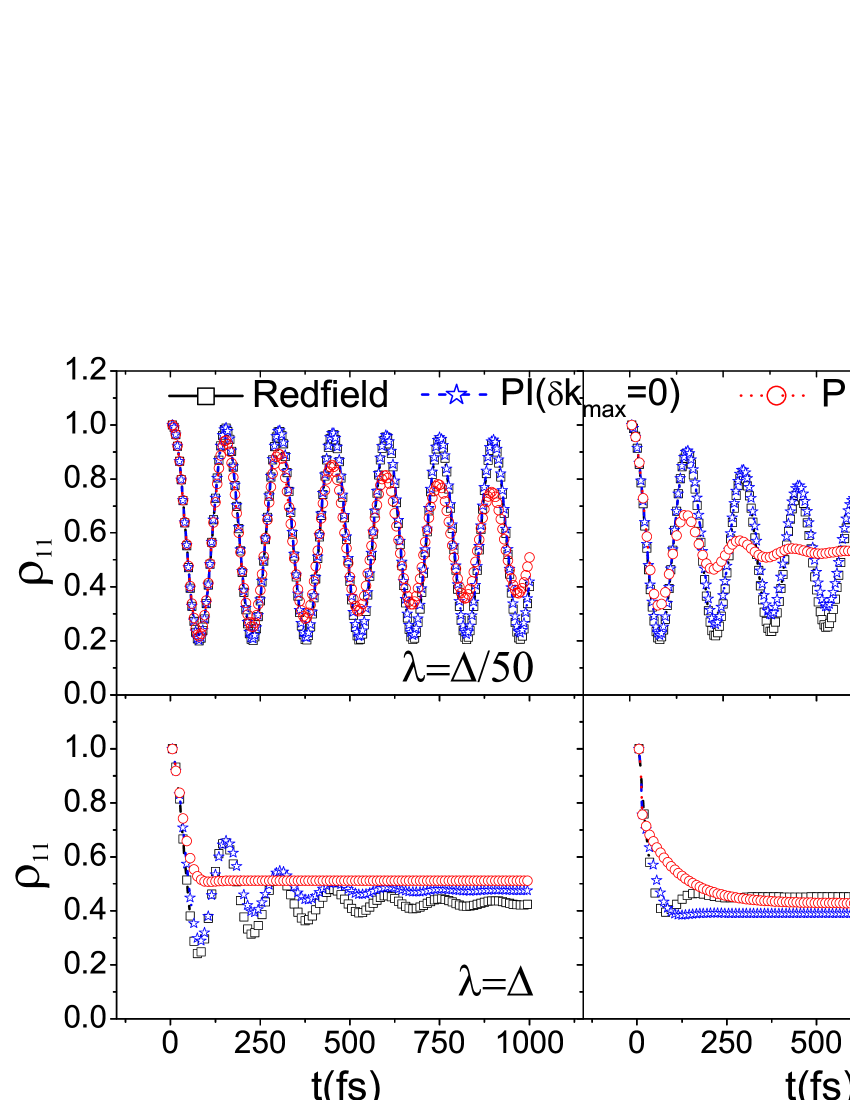
Figure 1: (Color online) Time evolutions of the population of site 1, obtained from master equations of Redfield form (black line connects black squares), and from ITM algorithm based on QUAPI of $\delta k_{max}=0$ (blue dashed line connects blue stars), and $\delta k_{max}=3$ (red dotted line connects red circles) for different $\lambda$. Here, $\epsilon=100$ cm${}^{-1},$ $\Delta=100$ cm${}^{-1},$ $\gamma=53.08$ cm^-1 ($\gamma^{-1}=100$ fs), and $T=300$ k. Initially, the system is populated on the site 1 with state $\left|\psi_{0}\right\rangle=\left|1\right\rangle$.

In Fig.1, we plot the time evolutions of the population of site 1 by using the master equations of Redfield form and the ITM algorithm as $\lambda=\Delta/50,\Delta/5,\Delta,$ and $5\Delta$. The initial state is $\left|\psi_{0}\right\rangle=\left|1\right\rangle$, where $\left|1\right\rangle$ is the basis state of the system. It is shown that the evolutions of the population of site 1 obtained from the master equations of Redfield form are in good agreement with the ones obtained from the ITM algorithm of $\delta k_{\max}=0$. We shall use $\delta k_{\max}=3,$ and $\delta t=10$ fs to investigate the dynamics under non-Markovian approximation in this paper, so in this case, the memory effects of the bath within $30$ fs are included. In fact, the memory time of the bath with Drude-Lorentz density function is longer than this value, the memory effects beyond $30$ fs will not be included in this paper. The time evolutions of the population of site 1 from ITM of $\delta k_{\max}=3,$ are also plotted in Fig.1 which is quite distinct from the Markovian results. It shows that when we investigate this kind of system the non-Markovian effects are non-ignorable. In the following, we shall use the ITM algorithm with $\delta k_{\max}=3$ to study the decoherence and the transfer rate of the EET. The memory effects of the bath have not been completely included in our calculations but the dominating affects have been included, because when we increase $\delta k_{\max}$ from $3$ to $4$ the results have little change and this change even cannot be distinguished by eyes.

III Time evolutions of coherence and EET

It is reported Engel ; Lee that the decoherence time of the coherent superposition state produced by laser pulses has the same time scale of the EET between two adjacent chromophores. People thus suppose that coherence may help the EET in photosynthesis. On the other hand, the theoretical analysis shows that the environment is not a hindrance but a help to the EET Plenio ; Mohseni . So, we want to know further that how the coherence helps the EET and how about non-Markovian environment compares to the Markovian one in the helps of the EET. In this section we shall discuss these kinds of problems through investigating above dynamical model to mimic photosynthesis systems.

Similar to Sec.II we can easily plot the evolution of the coherence, namely, the the evolution of the off-diagonal term in the reduced density matrix. It is also convenient to plot the evolution of the changing rate of population of site 2. The changing rate of the population of the site 2 in fact reflects the transfer rate of the EET from the site 1 to the site 2. Comparing the evolutions of the coherence and the transfer rate (denoted by $k$ in this paper) of the EET, we can judge whether the transfer rate of the EET increase or not as the coherence increase, and as the system in a non-Markovian environment instead of Markovian one.

In Figs.2 and 3 we plot the evolutions of the $\rho_{12}(t)$ and $k$ with time in different $\lambda$. Here we set $\lambda$ vary from $\Delta/5$, to $\Delta/4,\Delta/3,\Delta/2$, and $\epsilon=100$ cm${}^{-1},$ $\Delta=100$ cm${}^{-1}.$ In this paper we always set $\gamma=53.08$ cm^-1 ($\gamma^{-1}=100$ fs), and $T=300$ k. The initial state is set in the maximal coherent superposition state $\left|\psi_{0}\right\rangle=\left(\left|1\right\rangle+\left|2\right\rangle\right)/\sqrt{2}$ in Fig.2, and in the basis state $\left|\psi_{0}\right\rangle=\left|1\right\rangle$ in Fig.3. Figs.4 and 5 plot the evolutions of the $\rho_{12}(t)$ and $k$ with time t in different $\Delta$. Here, we set $\epsilon=100$ cm^-1, $\lambda=20$ cm^-1, and $\Delta$ vary from $\epsilon$, to $\epsilon/2,\epsilon/3$, and $\epsilon/4$, the initial state is $\left|\psi_{0}\right\rangle=\left(\left|1\right\rangle+\left|2\right\rangle\right)/\sqrt{2}$ in Fig.4, and $\left|\psi_{0}\right\rangle=\left|1\right\rangle$ in Fig.5. In the Figs.2-5, the time evolutions of the coherence are plotted in the upper panels (a) and (c) and transfer rate $k$ of the EET are plotted in the lower panels (b) and (d). In the left panels (a) and (b) are the results of Markovian approximation $\delta k_{\max}=0$, and in right panels (c) and (d) are the results of non-Markovian approximation $\delta k_{\max}=3$.

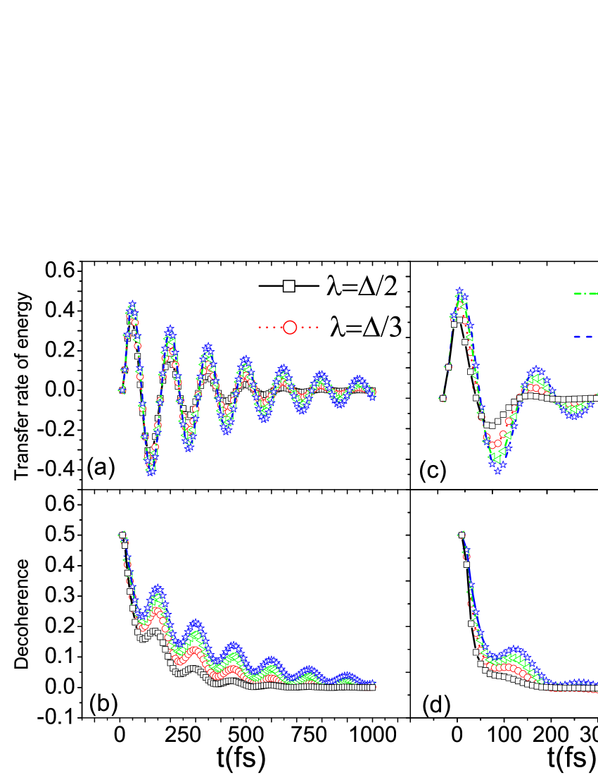
Figure 2: (Color online) Time evolutions of the coherence [upper panels (a) and (c)] and transfer rate of the EET [lower panels (b) and (d)], in Markovian approximation $\delta k_{\max}=0$ [left panels (a) and (b)], and in non-Markovian approximation $\delta k_{\max}=3$ [right panels (c) and (d)], for different values of $\lambda$. The initial state is $\left|\psi_{0}\right\rangle=\left(\left|1\right\rangle+\left|2\right\rangle\right)/\sqrt{2}$. The values of other parameters are the same as in Fig.1.

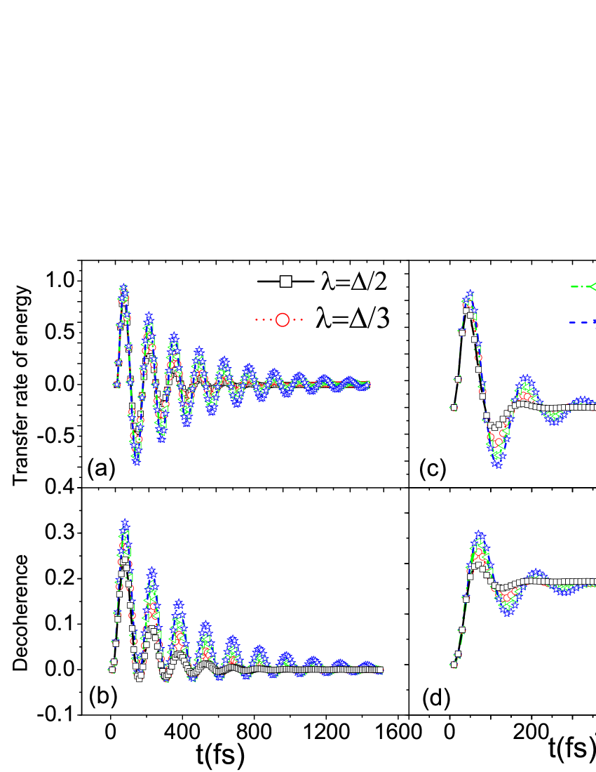
Figure 3: (Color online) Time evolutions of the coherence and transfer rate of the EET in Markovian and non-Markovian approximations. The parameters in Fig.3 are similar to them in Fig.2 except the initial state $\left|\psi_{0}\right\rangle=\left|1\right\rangle$.

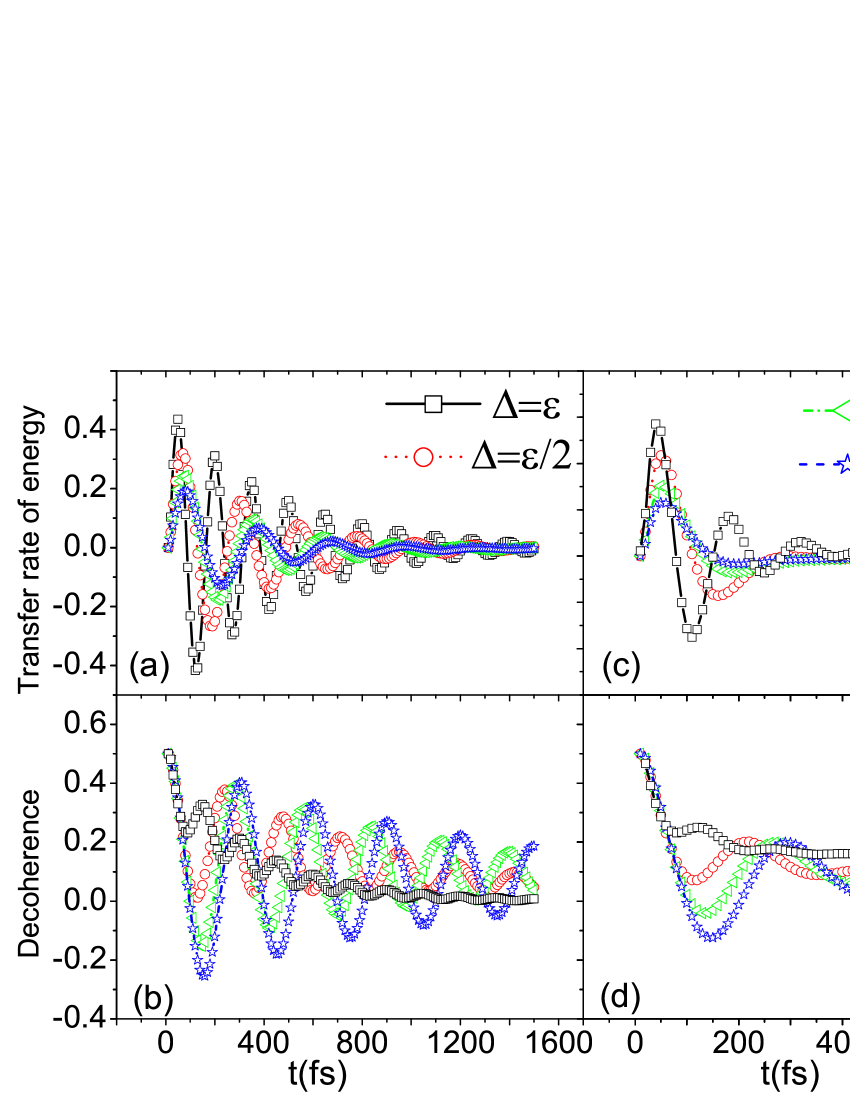
Figure 4: (Color online) Time evolutions of the coherence [upper panels (a) and (c)] and transfer rate of the EET [lower panels (b) and (d)], in Markovian approximation $\delta k_{\max}=0$ [left panels (a) and (b)], and in non-Markovian approximation $\delta k_{\max}=3$ [right panels (c) and (d)], for different values of $\Delta$. The initial state is $\left|\psi_{0}\right\rangle=\left(\left|1\right\rangle+\left|2\right\rangle\right)/\sqrt{2}$. The values of other parameters are the same as in Fig.1.

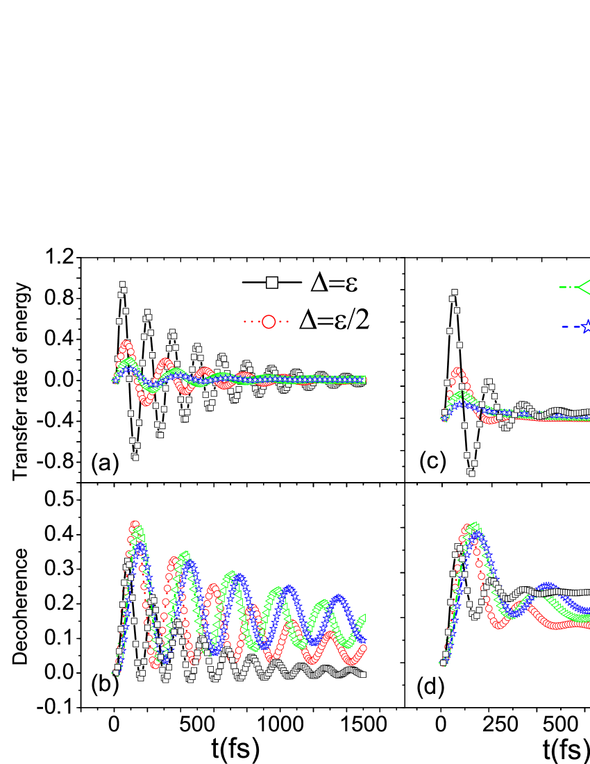
Figure 5: (Color online) Time evolutions of the coherence and transfer rate of the EET in Markovian and non-Markovian approximations. The parameters in Fig.5 are similar to them in Fig.4 except the initial state $\left|\psi_{0}\right\rangle=\left|1\right\rangle$.

Table 1: (Obtained from Figs.2 and 3) Transfer quantity of energy and decoherence times in different $\lambda$ as $\Delta=\epsilon=100$ cm^-1.

	$\left|\psi_{0}\right\rangle=\left(\left|1\right\rangle+\left|2\right\rangle\right)/\sqrt{2}$				$\left|\psi_{0}\right\rangle=\left|1\right\rangle$
	kmax=0		kmax=3		kmax=0		kmax=3
$\lambda$	$\tau$	area	$\tau$	area	$\tau$	area	$\tau$	area
$\Delta/5$	359	0.16098	almost same	0.44934	274	2.92073	almost same	3.44756
$\Delta/4$	265	0.08718		0.45430	390	2.96761		3.45388
$\Delta/3$	207	0.03219		0.46212	260	2.99283		3.46209
$\Delta/2$	149	0.00473		0.47830	240	2.99969		3.47830

Table 2: (Obtained from Figs. 4 and 5) Transfer quantity of energy and decoherence times in different $\Delta$ as $\epsilon=100$ cm^-1, $\lambda=\epsilon/5$.

	$\left|\psi_{0}\right\rangle=\left(\left|1\right\rangle+\left|2\right\rangle\right)/\sqrt{2}$				$\left|\psi_{0}\right\rangle=\left|1\right\rangle$
	kmax=0		kmax=3		kmax=0		kmax=3
$\Delta$	$\tau$	area	$\tau$	area	$\tau$	area	$\tau$	area
$\epsilon/2$	410	-0.02476	almost same	0.45031	800	2.92073	almost same	3.45018
$\epsilon/3$	870	0.09477		0.41073	830	2.90845		3.41011
$\epsilon/4$	1320	0.25661		0.41204	1380	2.62069		3.37671
$\epsilon/5$	1900	0.39017		0.43823	1700	2.18892		3.19348

The Table 1 is made by using the data of Figs.2 and 3, and the Table 2 is made from data of Figs.4 and 5. In the Tables 1 and 2 we numerically show the decoherence times and the net area of curve $k$ in different conditions. The positive value of transfer rate of the EET means that the energy transfers from the site 1 to the site 2, and the negative value of the $k$ means that it transfers back to the site 1 from the site 2. The net transfer quantity of energy from the site 1 to the site 2 is proportional to the net area under the curve $k$ (where the net area denote algebraic sum of the area). From Figs.2-5 and Tables 1 and 2 we can obtain the following results. (1) The transfer rate of energy $k$ from the site 1 to the site 2 are oscillations, the coherent term $\rho_{12}(t)$ are also oscillations. The two kinds of evolution curves almost have the same decay times. It means that the system is transferring the energy in all of the coherence time. However, the maximum of $k$ is nether at the maximal points nor at the minimal points of the curve $\rho_{12}(t)$. This means that the increase of coherence does not result in the increase of the transfer rate of the EET. Thus, we obtain the first conclusion in this paper that coherence helps the energy transfer through prolonging the transfer time rather than increase the transfer rate. As seen in the figures and tables that although the time of energy transfer is extended due to the increase of coherence its efficiency may decrease because the energy will be transferred between the site 1 and the site 2 back and forth. The breath-like transfer of energy in fact is ineffective. (2) From the Tables 1 and 2 we see that the environment really helps the energy transfer. It is clearly shown that an environment with stronger damping may stop the breath-like transfer of energy, which increase the transfer quality of the EET. In particular, as the non-Markovian effects are included the net area under the curve $k$, namely, the transfer quality of the EET is increased greatly in all cases. It means that the environment with non-Markovian effects will help the EET. This is the second conclusion in this paper. It is worthwhile to point out that as the initial state is the coherent superposition state the energy may be transferred from site 2 to 1 then the net area of the $k$ curve is negative as shown at 410 fs in Table 2.

IV Summary

To summary, in this paper we used a model introduced in Ref.Ishizaki-Fleming investigating the time evolutions of population by using the numerical path integral, which is qualitatively identical to the results obtained from reduced hierarchy equation approach in Ref.Ishizaki-Fleming . The path integral method includes the non-Markovian effects of bath. By use of the method we furthermore investigated the evolutions of the coherence and the transfer rate of the EET between two sites. We clearly show that there exist the energy transfer in all decoherence time. The increase of coherence does not directly result in the increase of the transfer rate of the EET. The helps of coherence to the energy transfer results from the increase of transfer time rather than the transfer rate. The energy transfer between two sites within first several hundred femtoseconds is like a breathing motion in Markovian environment. We have also obtained that the non-Markovian effects play important role to the dynamics of the energy transfer in the model systems in the initial several hundreds femtoseconds and it results in high efficiency of the EET. Our findings from spin-boson model study have important implications for understanding the energy transfer in photosynthesis systems.

- (1) May and O. Kuhn, Charge and Energy Transfer Dynamics in Molecular Systems, (Wiley, Weinheim, 2004); J. Cogdell, A. Gall, and J. Köhler, Q. Rev. Biophys. 39, 227 (2006); H. van Amerongen, L. Valkunas, and R. van Grondelle, Photosynthetic Excitons, (World Scientific, Singapore, 2000); J. Gilmore and R. H. MacKenzie, Chem. Phys. Lett. 421, 266 (2006).
- (2) R. E. Fenna and B. W. Matthews, Nature (London) 258, 573 (1975); Y.-F. Li, W. Zhou, R. E. Blankenship, and J. P. Allen, J. Mol. Biol. 271, 456 (1997).
- (3) As a review: X. Hu, K. Schulten, Phys. Today 50, 28 (1997) and references therein.
- (4) R. Van Grondelle, and V. Novoderezhkin, Phys. Chem. Chem. Phys. 8, 793 (2006).
- (5) G. S. Engel, T. R. Calhoun, E. L. Read, T.-K. Ahn, T. Mancal, Y.-C. Cheng, R. E. Blankenship, and G. R. Fleming, Nature (London) 446, 782 (2007).
- (6) H. Lee, Y.-C. Cheng, and G. R. Flemming, Science 316, 1462 (2007).
- (7) T. Förster, Ann Phys Leipzig 2, 55 (1948).
- (8) A. G. Redfield, IBM J. Res. Dev. 1, 19 (1957); A. G. Redfield, Adv. Magn. Reson. 1, 1 (1965); W. T. Pollard, A. K. Felts, and R. A. Friesner, Adv. Chem. Phys. 93, 77 (1996).
- (9) W. M. Zhang, T. Meier, V. Chernyak, and S. Mukamel, J. Chem. Phys. 108, 7763 (1998).
- (10) M. Yang, G. R.Fleming, Chem. Phys. 275, 355 (2002).
- (11) S. Jang, Y. Jung, R. J. Silbey, Chem. Phys. 275, 319 (2002).
- (12) A. Ishizaki, and G. R. Fleming, J. Chem. Phys. 130, 234110 (2009); ibid. 234111 (2009).
- (13) M. Mohseni, P. Rebentrost, S. Lloyd, and A. Aspuru-Guzik, J. Chem. Phys. 129, 174106 (2008); P. Rebentrost, M. Mohseni, I. Kassal, S. Lloyd, and A. Aspuru-Guzik, New J. Phys. 11, 033003 (2009).
- (14) M.B. Plenio and S.F. Huelga, New J. Phys. 10, 113019 (2008); F. Caruso, A. Chin, A. Datta, S.F. Huelga and M.B. Plenio, J. Chem. Phys. 131, 105106 (2009).
- (15) M. Thorwart, J. Eckel, J.H. Reina, P. Nalbach, and S. Weiss, Chem. Phys. Lett. 478, 234 (2009); J. Eckel, J.H. Reina, and M. Thorwart, New J. Phys. 11, 085001 (2009).
- (16) J. Ray and N. Makri, J. Phys. Chem. 103, 9417 (1999).
- (17) Z. G. Yu, M. A. Berding, and Haobin Wang, Phys. Rev. E 78, 050902(R) (2008).
- (18) A. Nazir, Phys. Rev. Lett. 103, 146404 (2009).
- (19) A. Damjanović, I. Kosztin, U. Kleinekathöfer, and K. Schulten,Phys. Rev. E 65, 031919 (2002).
- (20) M. W. Y. Tu, and W. -M. Zhang, Phys. Rev. B 78, 235311 (2008).
- (21) M. -T. Lee, and W. -M. Zhang, J. Chem. Phys. 129, 224106 (2008).
- (22) D. E. Makarov and N. Makri, Chem. Phys. Lett. 221, 482 (1994); N. Makri, and D. E. Makarov, J. Chem. Phys. 102, 4600; ibid. 102, 4611 (1995); N. Makri, E. Sim, D. E. Makarov, and M. Topaler, Proc. Natl. Acad. Sci. USA 93, 3926 (1996).
- (23) M. Thorwart, P. Reimann, and P. Hänggi, Phys. Rev. E 62, 5808 ( 2000); M. Thorwart, E. Paladino, M. Grifoni, Chem. Phys. 296, 333 (2004).
- (24) X. -T. Liang, Chem. Phys. Lett. 449, 296 (2007); X. -T. Liang, Chem. Phys. 352, 106 (2008); X. -T. Liang, Phys. Rev. B 72, 245328 (2005).