The Morphology of Urban Agglomerations for Developing Countries: A Case Study with China

Abstract

Abstract

In this article, the relationship between two well-accepted empirical propositions regarding the distribution of population in cities, namely, Gibrat’s law and Zipf’s law, are rigorously examined using the Chinese census data. Our findings are quite in contrast with the most of the previous studies performed exclusively for developed countries. This motivates us to build a general environment to explain the morphology of urban agglomerations both in developed and developing countries. A dynamic process of job creation generates a particular distribution for the urban agglomerations and introduction of Special Economic Zones (SEZ) in this abstract environment shows that the empirical observations are in good agreement with the proposed model.

I Introduction

Social phenomenon is a pertinent topic of discussion among the Economists and Econophysicists - partly because, human behavior can be explained in terms of Economic motives as well as a manifestation of a complex natural system. One of the interesting observation is distribution of dwellers in different urban agglomerations. A simple empirical law, namely Zipf’s law zipf , is often successful in describing the distribution of populations for various cities f1 in a nation.

In Economics, there is a body of literature devoted to explain morphology of cities. The survey paper by Gabaix and Ioannides gabaix_survey enlists most of them. Krugman krugman96 have looked at the top 135 U.S. cities and have found that the log-rank of a city bears a linear relation to the log-size of the same in a significant way. The slope of the linear relation is also found to be quite close to one as expected from the Zipf’s law.

Gabaix gabaix1999a investigate into the growth of cities and their adherence to the Zipf’s law. This is because Zipf’s law is not a static phenomenon, but is the outcome of a dynamic process. Different cities have presumably different growth processes. We can express the expected growth rate of a city with population $S$ as a random variable, $\mu(S)$. The standard deviation in the growth rate of cities with population $S$ are denoted by $\sigma(S)$. If either $\mu(S)$ or $\sigma(S)$ is a non-trivial function of $S$ at least in the upper tail of the distribution of $S$, there would be violations of Zipf’s law. This is a consequence of the Gibrat’s law being followed in the upper tail of the city distribution. Gibrat’s law proposes that the growth rate process of a city is independent of the size of the city. Therefore the mean growth rate and the standard deviation of the growth rate for a city is independent of its size. It must be clarified that Gibrat law does not say that the growth rate of any city follows the same stochastic process. It only says that there is no relation between growth rate of a city and its size.

Gibrat law and its relation to Zipf’s law is particularly pertinent for a nation experiencing growth in urban inhabitants. A developing country is very different compared to its developed counterparts in terms of economic and social structures. Therefore, the inter relationship between this two empirical conjectures might be particularly interesting. A pertinent case study is the People’s Republic of China, where urbanization is taking place in a fast pace. We investigate into the occurrence of these laws in case of China. The next section discusses our empirical analysis with the findings. A model is proposed in Section III along with an appropriate simulation study. The concluding remarks are noted in Section IV.

II Data Treatment

The People’s Republic of China conducted censuses in 1953, 1964, and 1982. At the 2000 census, the total population stood at approximately 1.29533 billion, which is about 22% of total population in the world. 36% of the Chinese population used to reside in urban agglomerations in 2000. We use the data china_data from 1990 and 2000 census (plotted in Fig. 1).

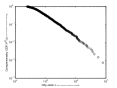
(a) Census year 1990: rank of a city plotted against its size

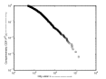
(b) Census year 2000: rank of a city plotted against its size

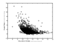
(c) Scatter plot of city growth against city size (1990-2000)

Figure 1: Chinese Cities: 1990-2000

II.1 Verification of Zipf’s Law

Let $p(\cdot)$ be a probability density function of the city-size distribution. The corresponding cumulative distribution function (CDF) and the complementary cumulative distribution function (CCDF) are given by $P(\cdot)$ and $P^{C}(\cdot)$, respectively. By definition,

$$P(x)=\int_{0}^{x}p(x^{\prime})dx^{\prime};~{}~{}~{}~{}P^{C}(x)=1-P(x)$$

In case of city-size distribution following the Zipf’s law,

$$p_{\alpha}(x)=Cx^{-\alpha}~{}~{}~{}\mbox{and}~{}~{}~{}\displaystyle P_{\alpha}^{C}(x)=\frac{C}{\alpha-1}x^{-(\alpha-1)}$$ (1)

where $\alpha$ and $C$ are constants. $\alpha$ is called the exponent of the power law. This family of power law distributions for $\alpha>1$ are known as the Pareto distribution. From equation (1), it is obvious that $p_{\alpha}(x)$ diverges to infinity for any value of $\alpha>1$ as $x\rightarrow 0$. Therefore, some minimum value, $x_{min}$, is usually considered for the support of the Pareto distribution.

Table 1: Data Description: Values of city-population are reported in units of thousands. The left truncation of the data is determined through the value of $x_{min}$. The numbers in parenthesis represent the standard errors for the estimates Source: china_data

Census	n	Min	Max	Mean	Median	First	Third	Estimate of $\alpha$
Year		Value	Value			Quartile	Quartile	Linear Fit	MLE
2000	1462	50.08	14230.99	298.27	136.63	80.86	265.42	1.7544	2.2975
								(0.0018)	(0.0572)
1990	1345	25.02	7821.79	156.33	68.71	44.23	128.96	1.7701	2.2308
								(0.0032)	(0.0736)

The slope of the plot, in which log of the rank of a city, $\log(R_{x})$, is plotted against the log of its population, $\log(x)$, has been used to estimate the exponent of the power law in almost all the previous studies. It has been shown shalizi_powerlaw ; gabaix1999a that this produces a biased estimate of the power law exponent. Alternatively the Maximum Likelihood Estimatorf2 The MLE is given by the expression, $\widehat{\alpha}_{MLE}=1+n\left[\sum_{i=1}^{n}\log\left(\frac{x_{i}}{x_{min}}\right)\right]^{-1}$ (MLE) produces the most efficient estimate. We find physica_2009 the estimate of $\alpha$ to be significantly bigger than 2 as a departure from the Zipf’s law (see Table 1).

II.2 Verification of Gibrat’s Law

The cities in the upper tail of the size distribution follow a constant rate of growth for various developed countries JanE_2004 . It is interesting to repeat this exercise for a developing nation, where urbanization is happening fast to notice any discrepancy among cities in terms of growth regarding size. We perform various non-parametric as well as parametric exercises on the data to find out the relationship between the size of of a city and its growth rate.

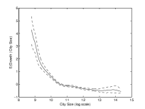
(a) Epanechnikov Kernel

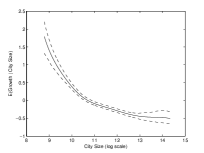
(b) Gaussian Kernel

Figure 2: Kernel estimates of population growth against city-size (dotted line represents the 95% bootstrapped confidence interval)

We plot the growth rate of population in all available urban agglomerations for the period of 1990-2000 against the population of the corresponding urban agglomeration in 1990. The standard non-parametric measure is to use the Kernel estimates of local mean. Suppose, the growth rate of a city, $g_{i}$, bears some relation with the size of the city, $S_{i}$, modeled as:

$$g_{i}=m(S_{i})+\epsilon_{i}$$

for all $i=1,2,...,n$, $n$ being the total number of cities with available data. The objective is to find a smooth estimate of local means of growth rate over size and to verify whether there is any visible relationship between growth and size based on this estimate $m(\cdot)$. $g_{i}$ is the growth rate of the $i$th city over 1990-2000. We perform a Kernel density regression in the support of $S_{i}$.f4 The local average smooths around the point $s$, and the smoothing is done using a kernel, i.e. a continuous weight function symmetric around $s$. The bandwidth $h$ of a kernel determines the scale of smoothing. The Nadaraya-Watson estimate Pagan_Ullah of $m(\cdot)$ is given by the following expression,

$$\hat{m}(s)=\frac{n^{-1}\sum_{i=1}^{n}K_{h}(s-S_{i})g_{i}}{n^{-1}\sum_{i=1}^{n}K_{h}(s-S_{i})}$$

We use two most popular Kernels, Gaussian and Epanechnikov. For Gaussian Kernel, $K(\psi)=(2\pi)^{-1/2}\exp\left[-\frac{1}{2}(\psi)^{2}\right]$, and for the Epanechnikov Kernel, $K(x)=\frac{3}{4}\left(1-\psi^{2}\right)\cdot\mathbf{1}_{|\psi|\leq 1}$. For both the kernels, we find that $m(\cdot)$ does depend on the size. The visual observation is verified through the following regression, where the growth rate of a city is regressed on the size of the city f3 . We find a significant f5 negative coefficient for the variable of city-size.

$$\begin{array}[]{l}g_{i}=2.635~{}~{}-~{}~{}4.681\times 10^{-7}\cdot\frac{S_{90}+S_{00}}{2}\\ ~{}~{}~{}~{}~{}(0.039)~{}~{}~{}~{}~{}(8.982\times 10^{-8})\end{array}$$

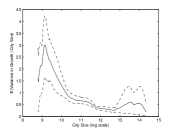
(a) Epanechnikov Kernel

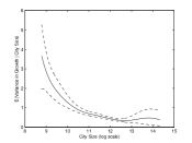
(b) Gaussian Kernel

Figure 3: Kernel estimates of variances in population growth against city-size (dotted line represents the 95% bootstrapped confidence interval)

We conclude that there is a definite variation among cities in terms of growth process and the overall evidence indicates that the growth process is negatively biased against the cities of higher sizes at least at the upper tail of the distribution.

III A Migration Based Model

To illustrate the empirical anomalies found in the context of distribution of urban agglomerations in China, we can motivate our findings with a mathematical model of city formation. There are several recent attempts batty ; beng ; witt to model urban growth. It uses the idea that the growth of cities resembles to that of the two-dimensional aggregates of particles. There are results in the the statistical physics of clusters regarding the growth of the two-dimensional aggregates of particles. These results are applied in the context of modeling the population distribution of urban agglomerations. In particular, the model of diffusion limited aggregation(DLA) predicted the existence of only one large fractal cluster that is almost perfectly screened from incoming development units so that almost all the cluster growth occurs in the extreme peripheral tips. The morphology of cities is also explained using a percolation modelmakse , where the scaling of the urban perimeter of individual cities and the distribution of system of cities are tested. The intermittency mechanismyb is used to modelzan a large scale city formation and understand the universal properties of the social phenomenon of city formation and global demographic development. In a different approachher , the laws of population growth is explained using the City Clustering Algorithm (CCA). The CCA is used to examine Gibrat’s law of proportional growth and finds that the mean growth rate of a cluster exhibits deviations from the Gibrat’s law.

For China, we need a model that is consistent with the empirical phenomenons observed and yet models the violations of the power law as found in the data. However, it must be taken into account that in the developed countries, this empirical observations are often reversed as we have found out from the literature. We introduce the aspect of Special Economic Zones in my model and explain the empirical anomalies in contrast to the developed countries in terms of Special Economic Zones. We construct a baseline environment without any Special Economic Zones. Then we add Special Economic Zones to that environment to observe any effect due to introduction of SEZ.

There are $k$ locations in a country. Jobs are spawn one at a time. The probability of a job being spawn in a location is a function number of already existing jobs in that location. More particularly, the probability of an additional job being created at the $i^{th}$ location is proportional to $n_{i}^{\gamma}$, where $n_{i}$ is the number of already existing jobs at the $i^{th}$ location. We let jobs spawn at different location until total number of jobs becomes $N$. The parameter $\gamma$ is an important parameter of scale. If $\gamma$ is 1, the growth rate of a city is independent of its size. On the other hand, if $\gamma$ is less than unity, larger cities are discriminated against regarding growth. A value of $\gamma$ being more than one means that the growth process favours the large cities to growth against the smaller cities.

We introduce a migration based Special Economic Zones in this model. The government introduce the feature of Special Economic Zones by giving special privileges to some cities. The privileged urban agglomerations are chosen in such a way that they are not from the most populous cities. A number of new jobs are created in the locations of the SEZs. These new jobs require higher skill levels compared to the previously existing jobs. A worker matched with these jobs leave their old locations of work and move to the new location. Also higher skilled workers are primarily from the top ranking cities.

III.1 A Simulation Study

To evaluate the performance of our economically tenable model, we resort to the widely used technique of simulation. We choose 3,000 locations ($k$) and one million agents ($N$). Jobs are spawn randomly in various locations are defined in our framework until the total number of spawned jobs is equal to total number of agents. We choose the value of $\gamma$ to be 0.9 so that there is a negative bias towards the growth of top ranking cities as observed as observed in the data. We consider the top 2,500 locations and estimate the power law coefficient using the maximum likelihood method. we find $\hat{\alpha}_{MLE}$ to be 1.0419 with standard error of the estimate being 0.0208.This baseline study is devoid of any SEZ and is quite in accordance with the Zipf’s Law.

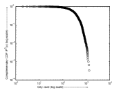
(a) Before introduction of SEZs, city sizes plotted against corresponding ranks

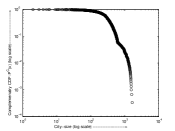
(b) After introduction of SEZs, city sizes plotted against corresponding ranks

Figure 4: Simulation study for the model

To introduce SEZ in this model, we randomly select 270 locations outside the top 300 locations and introduce a number of new jobs in those locations equaling 20% of already existing jobs in the economy. Workers from the top 300 locations are randomly matched with the newly created jobs and once matched, they migrate to the location of their new jobs. We compute $\hat{\alpha}_{MLE}$ in the same way considering top ranking 2,500 locations and find it to be 1.2667 with 0.0259 to be the standard error of the estimate. This is demonstrative of the high value of $\alpha$ estimated using the data for China. Moreover, $\alpha$ estimated for the census year of 2000 is higher than that for the census year of 1990. It is associated with the rising importance of SEZs in the Chinese economy.

IV Discussion

Economists often surmisegabaix_survey that Zipf’s law is the consequence of Gibrat’s law as far as city-size distribution is concerned. A simultaneous violation of both is natural. However, Gibrat’s law is associated with the free market economyjuan_carlos_cordoba . A breech in Gibrat’s law implies a wedge in the free market. A possible source of this wedge is debatable. We focus on government’s intervention on the natural process of morphology of cities. The cities under SEZ are subject to very different economic regulations compared to their counterparts in the rest of the country. This is analogous to a wedge in a perfectly competitive economic system.

It has been pointed outJanE_2004 that the Zipf’s exponent does depend on the cut-off in the upper tail of the city size distribution. The difference in socio-economic structure may give rise to different values of the Zipf’s exponent with the same minimum cut-off. It is observed that in case of China, the exponent of Zipf’s law augments for the year of 2000 compared to the value in the year of 1990. However, number of locations above the minimum cut-off are quite close (see Table 1). This phenomenon cannot be explained by a static process as modeled in JanE_2004 . Nevertheless, our model reconciles this empirical scenario with the gradual importance of SEZs in China.

References

- (1) G.K.Zipf, Human Behavior and the Principle of Least Effort (Addison-Wesley, Cambridge, MA, 1949)
- (2) In this article, “Urban Agglomeration” and “City” have throughout been used interchangeably. The literature starting from the Zipf’s law have historically looked into the population distribution of the urban areas formally denoted as “Cities”. However the more general notion of urban agglomerations have been used in the relatively recent literature.
- (3) The Evolution of City Size Distributions, Xavier Gabaix and Yannis Ioannides, Handbook of Regional and Urban Economics 4, V. Henderson and J-F. Thisse eds, 2004, North-Holland, 2341-2378.
- (4) The Self-Organizing Economy, (Blackwell Publishers Oxford, UK and Cambridge, MA).
- (5) Xavier Gabaix, Zipf s Law for Cities: An Explanation, Quarterly Journal of Economics 114 (3), August 1999, p.739-67.
- (6) Chinese Census data uploaded in http://www.citypopulation.de/China.html.
- (7) A. Clauset, C. R. Shalizi, and M. J. Newman, Power-law distributions in empirical data, arxiv:0706.1062v1.
- (8) The MLE is given by the expression,
- (9) Kausik Gangopadhyay and B. Basu, City Size Distribution for India and China, Physica A 388 (2009), 2682-2688.
- (10) Jan Eeckhout, Gibrat s Law for (all) Cities , American Economic Review 94(5), (2004), 1429-1451.
- (11) We have chosen the interval to exclude the effect of the boundaries to some extent.
- (12) Adrian Pagan and Aman Ullah, Nonparametric Econometrics, Cambridge University Press, 1999.
- (13) We choose the average of the populations in 1990 and 2000 at a city, respectively denoted as and , as the population of the city. We can however choose the population of the city in 1990 as the regression. The result is quite similar even quantitatively.
- (14) The standard errors of the estimates are shown in the parenthesis below.
- (15) M. Batty and P. Longley, Fractal Cities (Academic Press, San Diego, 1994)
- (16) L. Benguigui, A new aggregation model. Application to town growth, Physica A 219,(1995) 13
- (17) T.M. Witten and L.M. Sander, Diffusion-Limited Aggregation, a Kinetic Critical Phenomenon, Phys. Rev. Lett 47 (1981) 1400
- (18) H A. Makse et al. Modeling Urban Growth Patterns with Correlated Percolation, arXiv:cond-mat/9809431v1 [cond-mat.dis-nn], Phys. Rev. E (1 December 1998); Nature 377, 608 (1995)
- (19) Y.B. Zeldovich et al. The Almighty Chance (World Scientific, Singapore 1990)
- (20) D. H. Zanette and S.C. Manrubi, Role of Intermittency in Urban Development: A Model of Large-Scale City Formation, Phys. Rev. Lett. 79(1997) 523
- (21) H.D. Rozenfeld et. al.,Laws of population growth, arXiv:08082202
- (22) Juan Carlos Cordoba, On the Distribution of City Sizes, Journal of Urban Economics, January 2008.