I Introduction
In standard model (SM), the flavor changing neutral current (FCNC)
decays of B 𝐵 B B → K ∗ ( 892 ) γ → 𝐵 superscript 𝐾 892 𝛾 B\rightarrow K^{*}(892)\gamma Aubert:2004te ; Nakao:2004th ; Coan:1999kh B → K 1 ( 1270 , 1400 ) γ → 𝐵 subscript 𝐾 1 1270 1400 𝛾 B\rightarrow K_{1}(1270,1400)\gamma Yang:2004as B → K 0 ∗ ( 892 ) e + e − ( μ + μ − ) → 𝐵 superscript 𝐾 0
892 superscript 𝑒 superscript 𝑒 superscript 𝜇 superscript 𝜇 B\rightarrow K^{0*}(892)e^{+}e^{-}(\mu^{+}\mu^{-}) Ishikawa:2003cp ; Aubert:2006vb B → K ∗ ( 892 ) ℓ + ℓ − → 𝐵 superscript 𝐾 892 superscript ℓ superscript ℓ B\rightarrow K^{*}(892)\ell^{+}\ell^{-} Ishikawa:2006fh ; aubert:2008ju ; Aubert:2008ps K 1 ( 1270 , 1400 ) subscript 𝐾 1 1270 1400 K_{1}(1270,1400) BelleLH
ℬ ( B + → K 1 ( 1270 ) + γ ) ℬ → superscript 𝐵 subscript 𝐾 1 superscript 1270 𝛾 \displaystyle{\cal B}(B^{+}\rightarrow K_{1}(1270)^{+}\gamma) = \displaystyle= ( 4.28 ± 0.94 ± 0.43 ) × 10 − 5 , plus-or-minus 4.28 0.94 0.43 superscript 10 5 \displaystyle(4.28\pm 0.94\pm 0.43)\times 10^{-5},
ℬ ( B + → K 1 ( 1400 ) + γ ) ℬ → superscript 𝐵 subscript 𝐾 1 superscript 1400 𝛾 \displaystyle{\cal B}(B^{+}\rightarrow K_{1}(1400)^{+}\gamma) < \displaystyle< 1.44 × 10 − 5 . 1.44 superscript 10 5 \displaystyle 1.44\times 10^{-5}. (1)
The semileptonic B → K 1 ( 1270 , 1400 ) ℓ + ℓ − → 𝐵 subscript 𝐾 1 1270 1400 superscript ℓ superscript ℓ B\rightarrow K_{1}(1270,1400)\ell^{+}\ell^{-} B 𝐵 B b → s ℓ − ℓ + → 𝑏 𝑠 superscript ℓ superscript ℓ b\rightarrow s\ell^{-}\ell^{+} B → K 1 ( 1270 , 1400 ) ℓ + ℓ − → 𝐵 subscript 𝐾 1 1270 1400 superscript ℓ superscript ℓ B\rightarrow K_{1}(1270,1400)\ell^{+}\ell^{-} p p 𝑝 𝑝 pp e + e − superscript 𝑒 superscript 𝑒 e^{+}e^{-} LhcB superB LhcB2 V b t subscript 𝑉 𝑏 𝑡 V_{bt} V t s subscript 𝑉 𝑡 𝑠 V_{ts} B → K 1 ( 1270 , 1400 ) ℓ + ℓ − → 𝐵 subscript 𝐾 1 1270 1400 superscript ℓ superscript ℓ B\rightarrow K_{1}(1270,1400)\ell^{+}\ell^{-} yang87 ; hatanakayang ; gaur1 ; basihry ; vali-kazem ; Paracha:2007yx ; Ahmed:2008ti ; Saddique:2008xj ; lee K 1 ( 1270 , 1400 ) subscript 𝐾 1 1270 1400 K_{1}(1270,1400) yangana K 1 subscript 𝐾 1 K_{1} K 1 ( 1270 ) subscript 𝐾 1 1270 K_{1}(1270) K 1 ( 1400 ) subscript 𝐾 1 1400 K_{1}(1400) 1 3 P 1 ( K 1 A ) superscript 1 3 subscript 𝑃 1 subscript 𝐾 1 𝐴 {1^{3}P_{1}}(K_{1A}) 1 1 P 1 ( K 1 B ) superscript 1 1 subscript 𝑃 1 subscript 𝐾 1 𝐵 {1^{1}P_{1}}(K_{1B})
( | K 1 ( 1270 ) ⟩ | K 1 ( 1400 ) ⟩ ) = ℳ θ ( | K 1 A ⟩ | K 1 B ⟩ ) , ket subscript 𝐾 1 1270 ket subscript 𝐾 1 1400 subscript ℳ 𝜃 ket subscript 𝐾 1 𝐴 ket subscript 𝐾 1 𝐵 \left(\begin{array}[]{c}|{K_{1}(1270)}\rangle\\
|{K_{1}(1400)}\rangle\\
\end{array}\right)={\cal M}_{\theta}\left(\begin{array}[]{c}|{K_{1A}}\rangle\\
|{K_{1B}}\rangle\\
\end{array}\right), (2)
where
ℳ θ = ( sin θ K 1 cos θ K 1 cos θ K 1 − sin θ K 1 ) subscript ℳ 𝜃 subscript 𝜃 subscript 𝐾 1 subscript 𝜃 subscript 𝐾 1 subscript 𝜃 subscript 𝐾 1 subscript 𝜃 subscript 𝐾 1 {\cal M}_{\theta}=\left(\begin{array}[]{cc}\sin\theta_{K_{1}}&\cos\theta_{K_{1}}\\
\cos\theta_{K_{1}}&-\sin\theta_{K_{1}}\\
\end{array}\right) (3)
is the mixing matrix, and θ K 1 subscript 𝜃 subscript 𝐾 1 \theta_{K_{1}} cenk 34 ∘ ≤ | θ K 1 | ≤ 58 ∘ superscript 34 subscript 𝜃 subscript 𝐾 1 superscript 58 34^{\circ}\leq|\theta_{K_{1}}|\leq 58^{\circ} cenk ; Suzuki1 ; Burakovsky1997 θ K 1 subscript 𝜃 subscript 𝐾 1 \theta_{K_{1}} θ K 1 subscript 𝜃 subscript 𝐾 1 \theta_{K_{1}} B → K 1 ( 1270 ) γ → 𝐵 subscript 𝐾 1 1270 𝛾 B\rightarrow K_{1}(1270)\gamma τ → K 1 ( 1270 ) ν τ → 𝜏 subscript 𝐾 1 1270 subscript 𝜈 𝜏 \tau\rightarrow K_{1}(1270)\nu_{\tau} hatanakayang
θ K 1 = − ( 34 ± 13 ) ∘ . subscript 𝜃 subscript 𝐾 1 superscript plus-or-minus 34 13 \theta_{K_{1}}=-(34\pm 13)^{\circ}. (4)
In this
study, the results of hatanakayang MesRes K 1 ( 1270 ) subscript 𝐾 1 1270 K_{1}(1270)
In this work, we calculate the transition form factors of B → K 1 ( 1270 , 1400 ) ℓ + ℓ − → 𝐵 subscript 𝐾 1 1270 1400 superscript ℓ superscript ℓ B\rightarrow K_{1}(1270,1400)\ell^{+}\ell^{-} e + e − superscript 𝑒 superscript 𝑒 e^{+}e^{-} μ + μ − superscript 𝜇 superscript 𝜇 \mu^{+}\mu^{-} τ + τ − superscript 𝜏 superscript 𝜏 \tau^{+}\tau^{-}
This paper is organized as follows. In section 2 2 2 B → K 1 ( 1270 , 1400 ) ℓ + ℓ − → 𝐵 subscript 𝐾 1 1270 1400 superscript ℓ superscript ℓ B\rightarrow K_{1}(1270,1400)\ell^{+}\ell^{-} 3 3 3 3 3 3 4 4 4
II Defining B → K 1 ( 1270 , 1400 ) ℓ + ℓ − → 𝐵 subscript 𝐾 1 1270 1400 superscript ℓ superscript ℓ B\rightarrow K_{1}(1270,1400)\ell^{+}\ell^{-}
In SM the B → K 1 ℓ + ℓ − → 𝐵 subscript 𝐾 1 superscript ℓ superscript ℓ B\rightarrow K_{1}\ell^{+}\ell^{-} b → s ℓ + ℓ − → 𝑏 𝑠 superscript ℓ superscript ℓ b\rightarrow s\ell^{+}\ell^{-} 1 b → s ℓ + ℓ − → 𝑏 𝑠 superscript ℓ superscript ℓ b\rightarrow s\ell^{+}\ell^{-} gaur1
ℋ = G F α 2 2 π V t b V t s ∗ ℋ subscript 𝐺 𝐹 𝛼 2 2 𝜋 subscript 𝑉 𝑡 𝑏 subscript superscript 𝑉 𝑡 𝑠 \displaystyle{\cal H}=\frac{G_{F}\alpha}{2\sqrt{2}\pi}V_{tb}V^{*}_{ts} × \displaystyle\times { C 9 e f f s ¯ γ μ ( 1 − γ 5 ) b l ¯ γ μ l \displaystyle\Bigg{\{}C_{9}^{eff}\bar{s}\gamma_{\mu}(1-\gamma_{5})b\bar{l}\gamma_{\mu}l (5)
+ \displaystyle+ C 10 s ¯ γ μ ( 1 − γ 5 ) b l ¯ γ μ γ 5 l subscript 𝐶 10 ¯ 𝑠 subscript 𝛾 𝜇 1 subscript 𝛾 5 𝑏 ¯ 𝑙 subscript 𝛾 𝜇 subscript 𝛾 5 𝑙 \displaystyle C_{10}\bar{s}\gamma_{\mu}(1-\gamma_{5})b\bar{l}\gamma_{\mu}\gamma_{5}l
− \displaystyle- 2 C 7 e f f m b q 2 s ¯ σ μ ν q ν ( 1 + γ 5 ) b l ¯ γ μ l } , \displaystyle 2C_{7}^{eff}\frac{m^{b}}{q^{2}}\bar{s}\sigma_{\mu\nu}q^{\nu}(1+\gamma_{5})b\bar{l}\gamma_{\mu}l\Bigg{\}},
where C 7 e f f superscript subscript 𝐶 7 𝑒 𝑓 𝑓 C_{7}^{eff} C 9 e f f superscript subscript 𝐶 9 𝑒 𝑓 𝑓 C_{9}^{eff} C 10 subscript 𝐶 10 C_{10} G F subscript 𝐺 𝐹 G_{F} α 𝛼 \alpha Z 𝑍 Z V i j subscript 𝑉 𝑖 𝑗 V_{ij} q = p − p ′ 𝑞 𝑝 superscript 𝑝 ′ q=p-p^{\prime} 5 B → K 1 ℓ + ℓ − → 𝐵 subscript 𝐾 1 superscript ℓ superscript ℓ B\rightarrow K_{1}\ell^{+}\ell^{-}
ℳ = G F α 2 2 π V t b V t s ∗ ℳ subscript 𝐺 𝐹 𝛼 2 2 𝜋 subscript 𝑉 𝑡 𝑏 subscript superscript 𝑉 𝑡 𝑠 \displaystyle{\cal M}=\frac{G_{F}\alpha}{2\sqrt{2}\pi}V_{tb}V^{*}_{ts} × \displaystyle\times { C 9 e f f ⟨ K 1 ( p ′ , ϵ ) | s ¯ γ μ ( 1 − γ 5 ) b | B ( p ) ⟩ l ¯ γ μ l \displaystyle\Bigg{\{}C_{9}^{eff}\langle K_{1}(p^{\prime},\epsilon)|\bar{s}\gamma_{\mu}(1-\gamma_{5})b|B(p)\rangle\bar{l}\gamma_{\mu}l (6)
+ \displaystyle+ C 10 ⟨ K 1 ( p ′ , ϵ ) | s ¯ γ μ ( 1 − γ 5 ) b | B ( p ) ⟩ l ¯ γ μ γ 5 l subscript 𝐶 10 quantum-operator-product subscript 𝐾 1 superscript 𝑝 ′ italic-ϵ ¯ 𝑠 subscript 𝛾 𝜇 1 subscript 𝛾 5 𝑏 𝐵 𝑝 ¯ 𝑙 subscript 𝛾 𝜇 subscript 𝛾 5 𝑙 \displaystyle C_{10}\langle K_{1}(p^{\prime},\epsilon)|\bar{s}\gamma_{\mu}(1-\gamma_{5})b|B(p)\rangle\bar{l}\gamma_{\mu}\gamma_{5}l
− \displaystyle- 2 C 7 e f f m b q 2 ⟨ K 1 ( p ′ , ϵ ) | s ¯ σ μ ν q ν ( 1 + γ 5 ) b | B ( p ) ⟩ l ¯ γ μ l } , \displaystyle 2C_{7}^{eff}\frac{m^{b}}{q^{2}}\langle K_{1}(p^{\prime},\epsilon)|\bar{s}\sigma_{\mu\nu}q^{\nu}(1+\gamma_{5})b|B(p)\rangle\bar{l}\gamma_{\mu}l\Bigg{\}},
where p ( p ′ ) 𝑝 superscript 𝑝 ′ p(p^{\prime}) B ( K 1 ) 𝐵 subscript 𝐾 1 B(K_{1}) ϵ italic-ϵ \epsilon K 1 subscript 𝐾 1 K_{1} 6
⟨ K 1 ( p ′ , ϵ ) | s ¯ γ μ ( 1 − γ 5 ) b | B ( p ) ⟩ quantum-operator-product subscript 𝐾 1 superscript 𝑝 ′ italic-ϵ ¯ 𝑠 subscript 𝛾 𝜇 1 subscript 𝛾 5 𝑏 𝐵 𝑝 \displaystyle\langle K_{1}(p^{\prime},\epsilon)|\bar{s}\gamma_{\mu}(1-\gamma_{5})b|B(p)\rangle = \displaystyle= 2 i A ( q 2 ) M + m ε μ ν α β ϵ ∗ ν p α p ′ β − V 1 q 2 ( M + m ) ϵ μ ∗ 2 𝑖 𝐴 superscript 𝑞 2 𝑀 𝑚 subscript 𝜀 𝜇 𝜈 𝛼 𝛽 superscript italic-ϵ absent 𝜈 superscript 𝑝 𝛼 superscript 𝑝 ′ 𝛽
subscript 𝑉 1 superscript 𝑞 2 𝑀 𝑚 subscript superscript italic-ϵ 𝜇 \displaystyle\frac{2iA(q^{2})}{M+m}\varepsilon_{\mu\nu\alpha\beta}\epsilon^{*\nu}p^{\alpha}p^{\prime\beta}-V_{1}{q^{2}}(M+m)\epsilon^{*}_{\mu} (7)
+ \displaystyle+ V 2 ( q 2 ) M + m ( ϵ ∗ . p ) P μ + V 3 ( q 2 ) M + m ( ϵ ∗ . p ) q μ , \displaystyle\frac{V_{2}(q^{2})}{M+m}(\epsilon^{*}.p)P_{\mu}+\frac{V_{3}(q^{2})}{M+m}(\epsilon^{*}.p)q_{\mu}~{}~{},~{}~{}
⟨ K 1 ( p ′ , ϵ ) | s ¯ σ μ ν q ν ( 1 + γ 5 ) b | B ( p ) ⟩ quantum-operator-product subscript 𝐾 1 superscript 𝑝 ′ italic-ϵ ¯ 𝑠 subscript 𝜎 𝜇 𝜈 superscript 𝑞 𝜈 1 subscript 𝛾 5 𝑏 𝐵 𝑝 \displaystyle\langle K_{1}(p^{\prime},\epsilon)|\bar{s}\sigma_{\mu\nu}q^{\nu}(1+\gamma_{5})b|B(p)\rangle = \displaystyle= 2 T 1 ( q 2 ) ε μ ν α β ϵ ∗ ν p α p ′ β 2 subscript 𝑇 1 superscript 𝑞 2 subscript 𝜀 𝜇 𝜈 𝛼 𝛽 superscript italic-ϵ absent 𝜈 superscript 𝑝 𝛼 superscript 𝑝 ′ 𝛽
\displaystyle 2T_{1}(q^{2})\varepsilon_{\mu\nu\alpha\beta}\epsilon^{*\nu}p^{\alpha}p^{\prime\beta} (8)
− \displaystyle- i T 2 ( q 2 ) [ ( M 2 − m 2 ) ϵ μ ∗ − ( ϵ ∗ . p ) P μ ] \displaystyle iT_{2}(q^{2})[(M^{2}-m^{2})\epsilon^{*}_{\mu}-(\epsilon^{*}.p)P_{\mu}]
− \displaystyle- i T 3 ( q 2 ) ( ϵ ∗ . p ) [ q μ − q 2 P μ M 2 − m 2 ] , \displaystyle iT_{3}(q^{2})(\epsilon^{*}.p)\Bigg{[}q_{\mu}-\frac{q^{2}P_{\mu}}{M^{2}-m^{2}}\Bigg{]}~{}~{},~{}~{}
where P = p + p ′ 𝑃 𝑝 superscript 𝑝 ′ P=p+p^{\prime} M ≡ M B 𝑀 subscript 𝑀 𝐵 M\equiv M_{B} B 𝐵 B m ≡ m K 1 𝑚 subscript 𝑚 subscript 𝐾 1 m\equiv m_{K_{1}} K 1 subscript 𝐾 1 K_{1}
σ μ ν γ 5 = − i 2 ε μ ν α β σ α β subscript 𝜎 𝜇 𝜈 subscript 𝛾 5 𝑖 2 subscript 𝜀 𝜇 𝜈 𝛼 𝛽 subscript 𝜎 𝛼 𝛽 \sigma_{\mu\nu}\gamma_{5}=\frac{-i}{2}\varepsilon_{\mu\nu\alpha\beta}\sigma_{\alpha\beta} (9)
with the convention γ 5 = i γ 0 γ 1 γ 2 γ 3 subscript 𝛾 5 𝑖 subscript 𝛾 0 subscript 𝛾 1 subscript 𝛾 2 subscript 𝛾 3 \gamma_{5}=i\gamma_{0}\gamma_{1}\gamma_{2}\gamma_{3} ε 0123 = − 1 subscript 𝜀 0123 1 \varepsilon_{0123}=-1 T 1 ( 0 ) = T 2 ( 0 ) subscript 𝑇 1 0 subscript 𝑇 2 0 T_{1}(0)=T_{2}(0) hatanakayang ; gaur1 ; cenk 1
Table 1: The relation of form
factors used in this work, and used in
literaturehatanakayang ; gaur1 ; cenk
In this work the branching fractions of B → K 1 ( 1270 , 1400 ) ℓ + ℓ − → 𝐵 subscript 𝐾 1 1270 1400 superscript ℓ superscript ℓ B\rightarrow K_{1}(1270,1400)\ell^{+}\ell^{-} B 𝐵 B 6
d Γ d q ^ = G F 2 α 2 M 2 14 π 5 | V t b V t s ∗ | 2 λ 1 / 2 ( 1 , r ^ , q ^ ) v Δ ( q ^ ) , 𝑑 Γ 𝑑 ^ 𝑞 superscript subscript 𝐺 𝐹 2 superscript 𝛼 2 𝑀 superscript 2 14 superscript 𝜋 5 superscript subscript 𝑉 𝑡 𝑏 superscript subscript 𝑉 𝑡 𝑠 2 superscript 𝜆 1 2 1 ^ 𝑟 ^ 𝑞 𝑣 Δ ^ 𝑞 \frac{d\Gamma}{d\hat{q}}=\frac{G_{F}^{2}\alpha^{2}M}{2^{14}\pi^{5}}|V_{tb}V_{ts}^{*}|^{2}\lambda^{1/2}(1,\hat{r},\hat{q})v\Delta(\hat{q})~{}, (10)
where q ^ = q 2 / M 2 ^ 𝑞 superscript 𝑞 2 superscript 𝑀 2 \hat{q}=q^{2}/M^{2} λ ( a , b , c ) = a 2 + b 2 + c 2 − 2 ( a b + b c + c a ) 𝜆 𝑎 𝑏 𝑐 superscript 𝑎 2 superscript 𝑏 2 superscript 𝑐 2 2 𝑎 𝑏 𝑏 𝑐 𝑐 𝑎 \lambda(a,b,c)=a^{2}+b^{2}+c^{2}-2(ab+bc+ca)
Δ ( q ^ ) Δ ^ 𝑞 \displaystyle\Delta(\hat{q}) = \displaystyle= 2 3 r ^ q ^ M 2 R e [ − 12 M 2 m ^ l q ^ λ ( 1 , r ^ , q ^ ) { ( ℰ 3 − 𝒟 2 − 𝒟 3 ) ℰ 1 ∗ \displaystyle\frac{2}{3\hat{r}\hat{q}}M^{2}Re\Big{[}-12M^{2}\hat{m}_{l}\hat{q}\lambda(1,\hat{r},\hat{q})\Big{\{}({\cal E}_{3}-{\cal D}_{2}-{\cal D}_{3}){\cal E}_{1}^{\ast} (11)
− \displaystyle- ( ℰ 2 + ℰ 3 − 𝒟 3 ) 𝒟 1 ∗ } + 12 M 4 m ^ l q ^ ( 1 − r ^ ) λ ( 1 , r ^ , q ^ ) ( ℰ 2 − 𝒟 2 ) ( ℰ 3 ∗ − 𝒟 3 ∗ ) \displaystyle({\cal E}_{2}+{\cal E}_{3}-{\cal D}_{3}){\cal D}_{1}^{\ast}\Big{\}}+12M^{4}\hat{m}_{l}\hat{q}(1-\hat{r})\lambda(1,\hat{r},\hat{q})({\cal E}_{2}-{\cal D}_{2})({\cal E}_{3}^{\ast}-{\cal D}_{3}^{\ast})
+ \displaystyle+ 48 m ^ l r ^ q ^ { 3 ℰ 1 𝒟 1 ∗ + 2 M 4 λ ( 1 , r ^ , q ^ ) ℰ 0 𝒟 0 ∗ } − 16 M 4 r ^ q ^ ( m ^ l − q ^ ) λ ( 1 , r ^ , q ^ ) { | ℰ 0 | 2 + | 𝒟 0 | 2 } 48 subscript ^ 𝑚 𝑙 ^ 𝑟 ^ 𝑞 3 subscript ℰ 1 superscript subscript 𝒟 1 ∗ 2 superscript 𝑀 4 𝜆 1 ^ 𝑟 ^ 𝑞 subscript ℰ 0 superscript subscript 𝒟 0 ∗ 16 superscript 𝑀 4 ^ 𝑟 ^ 𝑞 subscript ^ 𝑚 𝑙 ^ 𝑞 𝜆 1 ^ 𝑟 ^ 𝑞 superscript subscript ℰ 0 2 superscript subscript 𝒟 0 2 \displaystyle 48\hat{m}_{l}\hat{r}\hat{q}\Big{\{}3{\cal E}_{1}{\cal D}_{1}^{\ast}+2M^{4}\lambda(1,\hat{r},\hat{q}){\cal E}_{0}{\cal D}_{0}^{\ast}\Big{\}}-16M^{4}\hat{r}\hat{q}(\hat{m}_{l}-\hat{q})\lambda(1,\hat{r},\hat{q})\Big{\{}|{\cal E}_{0}|^{2}+|{\cal D}_{0}|^{2}\Big{\}}
− \displaystyle- 6 M 4 m ^ l q ^ λ ( 1 , r ^ , q ^ ) { 2 ( 2 + 2 r ^ − q ^ ) ℰ 2 𝒟 2 ∗ − q ^ | ( ℰ 3 − 𝒟 3 ) | 2 } 6 superscript 𝑀 4 subscript ^ 𝑚 𝑙 ^ 𝑞 𝜆 1 ^ 𝑟 ^ 𝑞 2 2 2 ^ 𝑟 ^ 𝑞 subscript ℰ 2 superscript subscript 𝒟 2 ∗ ^ 𝑞 superscript subscript ℰ 3 subscript 𝒟 3 2 \displaystyle 6M^{4}\hat{m}_{l}\hat{q}\lambda(1,\hat{r},\hat{q})\Big{\{}2(2+2\hat{r}-\hat{q}){\cal E}_{2}{\cal D}_{2}^{\ast}-\hat{q}|({\cal E}_{3}-{\cal D}_{3})|^{2}\Big{\}}
− \displaystyle- 4 M 2 λ ( 1 , r ^ , q ^ ) { m ^ l ( 2 − 2 r ^ + q ^ ) + q ^ ( 1 − r ^ − q ^ ) } ( ℰ 1 ℰ 2 ∗ + 𝒟 1 𝒟 2 ∗ ) 4 superscript 𝑀 2 𝜆 1 ^ 𝑟 ^ 𝑞 subscript ^ 𝑚 𝑙 2 2 ^ 𝑟 ^ 𝑞 ^ 𝑞 1 ^ 𝑟 ^ 𝑞 subscript ℰ 1 superscript subscript ℰ 2 ∗ subscript 𝒟 1 superscript subscript 𝒟 2 ∗ \displaystyle 4M^{2}\lambda(1,\hat{r},\hat{q})\Big{\{}\hat{m}_{l}(2-2\hat{r}+\hat{q})+\hat{q}(1-\hat{r}-\hat{q})\Big{\}}({\cal E}_{1}{\cal E}_{2}^{\ast}+{\cal D}_{1}{\cal D}_{2}^{\ast})
+ \displaystyle+ q ^ { 6 r ^ q ^ ( 3 + v 2 ) + λ ( 1 , r ^ , q ^ ) ( 3 − v 2 ) } { | ℰ 1 | 2 + | 𝒟 1 | 2 } ^ 𝑞 6 ^ 𝑟 ^ 𝑞 3 superscript 𝑣 2 𝜆 1 ^ 𝑟 ^ 𝑞 3 superscript 𝑣 2 superscript subscript ℰ 1 2 superscript subscript 𝒟 1 2 \displaystyle\hat{q}\Big{\{}6\hat{r}\hat{q}(3+v^{2})+\lambda(1,\hat{r},\hat{q})(3-v^{2})\Big{\}}\Big{\{}|{\cal E}_{1}|^{2}+|{\cal D}_{1}|^{2}\Big{\}}
− \displaystyle- 2 M 4 λ ( 1 , r ^ , q ^ ) { m ^ l [ λ ( 1 , r ^ , q ^ ) − 3 ( 1 − r ^ ) 2 ] − λ ( 1 , r ^ , q ^ ) q ^ } { | ℰ 2 | 2 + | 𝒟 2 | 2 } ] , \displaystyle 2M^{4}\lambda(1,\hat{r},\hat{q})\Big{\{}\hat{m}_{l}[\lambda(1,\hat{r},\hat{q})-3(1-\hat{r})^{2}]-\lambda(1,\hat{r},\hat{q})\hat{q}\Big{\}}\Big{\{}|{\cal E}_{2}|^{2}+|{\cal D}_{2}|^{2}\Big{\}}\Big{]}~{},
and r ^ = m 2 / M 2 ^ 𝑟 superscript 𝑚 2 superscript 𝑀 2 \hat{r}=m^{2}/M^{2} m ^ l = m l 2 / M 2 subscript ^ 𝑚 𝑙 superscript subscript 𝑚 𝑙 2 superscript 𝑀 2 \hat{m}_{l}=m_{l}^{2}/M^{2} v = 1 − 4 m ^ l / q ^ 𝑣 1 4 subscript ^ 𝑚 𝑙 ^ 𝑞 v=\sqrt{1-4\hat{m}_{l}/\hat{q}}
𝒟 0 subscript 𝒟 0 \displaystyle{\cal D}_{0} = \displaystyle= ( C 9 e f f + C 10 ) A ( q 2 ) M + m + ( 2 m b C 7 e f f ) T 1 ( q 2 ) q 2 , superscript subscript 𝐶 9 𝑒 𝑓 𝑓 subscript 𝐶 10 𝐴 superscript 𝑞 2 𝑀 𝑚 2 subscript 𝑚 𝑏 superscript subscript 𝐶 7 𝑒 𝑓 𝑓 subscript 𝑇 1 superscript 𝑞 2 superscript 𝑞 2 \displaystyle(C_{9}^{eff}+C_{10})\frac{A(q^{2})}{M+m}+(2m_{b}C_{7}^{eff})\frac{T_{1}(q^{2})}{q^{2}}~{},
𝒟 1 subscript 𝒟 1 \displaystyle{\cal D}_{1} = \displaystyle= ( C 9 e f f + C 10 ) ( M + m ) V 1 ( q 2 ) + ( 2 m b C 7 e f f ) ( M 2 − m 2 ) T 2 ( q 2 ) q 2 , superscript subscript 𝐶 9 𝑒 𝑓 𝑓 subscript 𝐶 10 𝑀 𝑚 subscript 𝑉 1 superscript 𝑞 2 2 subscript 𝑚 𝑏 superscript subscript 𝐶 7 𝑒 𝑓 𝑓 superscript 𝑀 2 superscript 𝑚 2 subscript 𝑇 2 superscript 𝑞 2 superscript 𝑞 2 \displaystyle(C_{9}^{eff}+C_{10})(M+m)V_{1}(q^{2})+(2m_{b}C_{7}^{eff})(M^{2}-m^{2})\frac{T_{2}(q^{2})}{q^{2}}~{},
𝒟 2 subscript 𝒟 2 \displaystyle{\cal D}_{2} = \displaystyle= C 9 e f f + C 10 M + m V 2 ( q 2 ) + ( 2 m b C 7 e f f ) 1 q 2 [ T 2 ( q 2 ) + q 2 M 2 − m 2 T 3 ( q 2 ) ] , superscript subscript 𝐶 9 𝑒 𝑓 𝑓 subscript 𝐶 10 𝑀 𝑚 subscript 𝑉 2 superscript 𝑞 2 2 subscript 𝑚 𝑏 superscript subscript 𝐶 7 𝑒 𝑓 𝑓 1 superscript 𝑞 2 delimited-[] subscript 𝑇 2 superscript 𝑞 2 superscript 𝑞 2 superscript 𝑀 2 superscript 𝑚 2 subscript 𝑇 3 superscript 𝑞 2 \displaystyle\frac{C_{9}^{eff}+C_{10}}{M+m}V_{2}(q^{2})+(2m_{b}C_{7}^{eff})\frac{1}{q^{2}}\left[T_{2}(q^{2})+\frac{q^{2}}{M^{2}-m^{2}}T_{3}(q^{2})\right]~{},
𝒟 3 subscript 𝒟 3 \displaystyle{\cal D}_{3} = \displaystyle= ( C 9 e f f + C 10 ) V 3 ( q 2 ) M + m − ( 2 m b C 7 e f f ) T 3 ( q 2 ) q 2 , superscript subscript 𝐶 9 𝑒 𝑓 𝑓 subscript 𝐶 10 subscript 𝑉 3 superscript 𝑞 2 𝑀 𝑚 2 subscript 𝑚 𝑏 superscript subscript 𝐶 7 𝑒 𝑓 𝑓 subscript 𝑇 3 superscript 𝑞 2 superscript 𝑞 2 \displaystyle(C_{9}^{eff}+C_{10})\frac{V_{3}(q^{2})}{M+m}-(2m_{b}C_{7}^{eff})\frac{T_{3}(q^{2})}{q^{2}}~{},
ℰ 0 subscript ℰ 0 \displaystyle{\cal E}_{0} = \displaystyle= ( C 9 e f f − C 10 ) A ( q 2 ) M + m + ( 2 m b C 7 e f f ) T 3 ( q 2 ) q 2 , superscript subscript 𝐶 9 𝑒 𝑓 𝑓 subscript 𝐶 10 𝐴 superscript 𝑞 2 𝑀 𝑚 2 subscript 𝑚 𝑏 superscript subscript 𝐶 7 𝑒 𝑓 𝑓 subscript 𝑇 3 superscript 𝑞 2 superscript 𝑞 2 \displaystyle(C_{9}^{eff}-C_{10})\frac{A(q^{2})}{M+m}+(2m_{b}C_{7}^{eff})\frac{T_{3}(q^{2})}{q^{2}}~{},
ℰ 1 subscript ℰ 1 \displaystyle{\cal E}_{1} = \displaystyle= ( C 9 e f f − C 10 ) ( M + m ) V 1 ( q 2 ) + ( 2 m b C 7 e f f ) ( M 2 − m 2 ) T 2 ( q 2 ) q 2 , superscript subscript 𝐶 9 𝑒 𝑓 𝑓 subscript 𝐶 10 𝑀 𝑚 subscript 𝑉 1 superscript 𝑞 2 2 subscript 𝑚 𝑏 superscript subscript 𝐶 7 𝑒 𝑓 𝑓 superscript 𝑀 2 superscript 𝑚 2 subscript 𝑇 2 superscript 𝑞 2 superscript 𝑞 2 \displaystyle(C_{9}^{eff}-C_{10})(M+m)V_{1}(q^{2})+(2m_{b}C_{7}^{eff})(M^{2}-m^{2})\frac{T_{2}(q^{2})}{q^{2}}~{},
ℰ 2 subscript ℰ 2 \displaystyle{\cal E}_{2} = \displaystyle= C 9 e f f − C 10 M + m V 2 ( q 2 ) + ( 2 m b C 7 e f f ) 1 q 2 [ T 2 ( q 2 ) + q 2 M 2 − m 2 T 3 ( q 2 ) ] , superscript subscript 𝐶 9 𝑒 𝑓 𝑓 subscript 𝐶 10 𝑀 𝑚 subscript 𝑉 2 superscript 𝑞 2 2 subscript 𝑚 𝑏 superscript subscript 𝐶 7 𝑒 𝑓 𝑓 1 superscript 𝑞 2 delimited-[] subscript 𝑇 2 superscript 𝑞 2 superscript 𝑞 2 superscript 𝑀 2 superscript 𝑚 2 subscript 𝑇 3 superscript 𝑞 2 \displaystyle\frac{C_{9}^{eff}-C_{10}}{M+m}V_{2}(q^{2})+(2m_{b}C_{7}^{eff})\frac{1}{q^{2}}\left[T_{2}(q^{2})+\frac{q^{2}}{M^{2}-m^{2}}T_{3}(q^{2})\right]~{},
ℰ 3 subscript ℰ 3 \displaystyle{\cal E}_{3} = \displaystyle= ( C 9 e f f − C 10 ) V 3 ( q 2 ) M + m − ( 2 m b C 7 e f f ) T 3 ( q 2 ) q 2 . superscript subscript 𝐶 9 𝑒 𝑓 𝑓 subscript 𝐶 10 subscript 𝑉 3 superscript 𝑞 2 𝑀 𝑚 2 subscript 𝑚 𝑏 superscript subscript 𝐶 7 𝑒 𝑓 𝑓 subscript 𝑇 3 superscript 𝑞 2 superscript 𝑞 2 \displaystyle(C_{9}^{eff}-C_{10})\frac{V_{3}(q^{2})}{M+m}-(2m_{b}C_{7}^{eff})\frac{T_{3}(q^{2})}{q^{2}}.
III Sum rules for B → K 1 ( 1270 , 1400 ) ℓ + ℓ − → 𝐵 subscript 𝐾 1 1270 1400 superscript ℓ superscript ℓ B\rightarrow K_{1}(1270,1400)\ell^{+}\ell^{-}
In this section the sum rules for the form factors of B → K 1 ( 1270 , 1400 ) ℓ + ℓ − → 𝐵 subscript 𝐾 1 1270 1400 superscript ℓ superscript ℓ B\rightarrow K_{1}(1270,1400)\ell^{+}\ell^{-} 7 8
Π μ ν A , a ( p 2 , p ′ 2 ) subscript superscript Π 𝐴 𝑎
𝜇 𝜈 superscript 𝑝 2 superscript 𝑝 ′ 2
\displaystyle\Pi^{A,a}_{\mu\nu}(p^{2},p^{\prime 2}) = \displaystyle= i 2 ∫ 𝑑 x 4 𝑑 y 4 e − i p x e i p ′ y ⟨ 0 | T [ J ν A ( y ) J μ a ( 0 ) J B † ( x ) ] | 0 ⟩ , superscript 𝑖 2 differential-d superscript 𝑥 4 differential-d superscript 𝑦 4 superscript 𝑒 𝑖 𝑝 𝑥 superscript 𝑒 𝑖 superscript 𝑝 ′ 𝑦 quantum-operator-product 0 𝑇 delimited-[] subscript superscript 𝐽 𝐴 𝜈 𝑦 subscript superscript 𝐽 𝑎 𝜇 0 superscript subscript 𝐽 𝐵 † 𝑥 0 \displaystyle i^{2}\int dx^{4}dy^{4}e^{-ipx}e^{ip^{\prime}y}\langle{0}|T[J^{A}_{\nu}(y)J^{a}_{\mu}(0)J_{B}^{\dagger}(x)]|{0}\rangle,
Π μ ν ρ T , a ( p 2 , p ′ 2 ) subscript superscript Π 𝑇 𝑎
𝜇 𝜈 𝜌 superscript 𝑝 2 superscript 𝑝 ′ 2
\displaystyle\Pi^{T,a}_{\mu\nu\rho}(p^{2},p^{\prime 2}) = \displaystyle= i 2 ∫ 𝑑 x 4 𝑑 y 4 e − i p x e i p ′ y ⟨ 0 | T [ J ν ρ T ( y ) J μ a ( 0 ) J B † ( x ) ] | 0 ⟩ , superscript 𝑖 2 differential-d superscript 𝑥 4 differential-d superscript 𝑦 4 superscript 𝑒 𝑖 𝑝 𝑥 superscript 𝑒 𝑖 superscript 𝑝 ′ 𝑦 quantum-operator-product 0 𝑇 delimited-[] subscript superscript 𝐽 𝑇 𝜈 𝜌 𝑦 subscript superscript 𝐽 𝑎 𝜇 0 superscript subscript 𝐽 𝐵 † 𝑥 0 \displaystyle i^{2}\int dx^{4}dy^{4}e^{-ipx}e^{ip^{\prime}y}\langle{0}|T[J^{T}_{\nu\rho}(y)J^{a}_{\mu}(0)J_{B}^{\dagger}(x)]|{0}\rangle, (13)
where J ν A = s ¯ γ ν γ 5 d subscript superscript 𝐽 𝐴 𝜈 ¯ 𝑠 subscript 𝛾 𝜈 subscript 𝛾 5 𝑑 J^{A}_{\nu}=\bar{s}\gamma_{\nu}\gamma_{5}d J ν ρ T = s ¯ σ ν ρ γ 5 d subscript superscript 𝐽 𝑇 𝜈 𝜌 ¯ 𝑠 subscript 𝜎 𝜈 𝜌 subscript 𝛾 5 𝑑 J^{T}_{\nu\rho}=\bar{s}\sigma_{\nu\rho}\gamma_{5}d K 1 subscript 𝐾 1 K_{1} J B = b ¯ γ 5 d subscript 𝐽 𝐵 ¯ 𝑏 subscript 𝛾 5 𝑑 J_{B}=\bar{b}\gamma_{5}d B 𝐵 B J μ a = J μ V − A , T + P T subscript superscript 𝐽 𝑎 𝜇 superscript subscript 𝐽 𝜇 𝑉 𝐴 𝑇 𝑃 𝑇
J^{a}_{\mu}=J_{\mu}^{V-A,T+PT} J μ V − A = b ¯ γ μ ( 1 − γ 5 ) s superscript subscript 𝐽 𝜇 𝑉 𝐴 ¯ 𝑏 subscript 𝛾 𝜇 1 subscript 𝛾 5 𝑠 J_{\mu}^{V-A}=\bar{b}\gamma_{\mu}(1-\gamma_{5})s J T + P T = b ¯ σ μ ϱ q ϱ ( 1 + γ 5 ) s superscript 𝐽 𝑇 𝑃 𝑇 ¯ 𝑏 subscript 𝜎 𝜇 italic-ϱ superscript 𝑞 italic-ϱ 1 subscript 𝛾 5 𝑠 J^{T+PT}=\bar{b}\sigma_{\mu\varrho}q^{\varrho}(1+\gamma_{5})s
The correlators are calculated in the following way. First, they are
saturated with two complete sets of intermediate states with same
quantum numbers of the initial and final state currents. These
calculations in terms of the matrix elements of K 1 ( 1270 ) subscript 𝐾 1 1270 K_{1}(1270) K 1 ( 1400 ) subscript 𝐾 1 1400 K_{1}(1400) III
Π μ ν A , a ( p 2 , p ′ 2 ) subscript superscript Π 𝐴 𝑎
𝜇 𝜈 superscript 𝑝 2 superscript 𝑝 ′ 2
\displaystyle\Pi^{A,a}_{\mu\nu}(p^{2},p^{\prime 2}) = \displaystyle= − ⟨ 0 | J ν A | K 1 ( 1270 ) ( p ′ , ϵ ) ⟩ ⟨ K 1 ( 1270 ) ( p ′ , ϵ ) | J μ a | B ( p ) ⟩ ⟨ B ( p ) | J B | 0 ⟩ R 1 R quantum-operator-product 0 subscript superscript 𝐽 𝐴 𝜈 subscript 𝐾 1 1270 superscript 𝑝 ′ italic-ϵ quantum-operator-product subscript 𝐾 1 1270 superscript 𝑝 ′ italic-ϵ subscript superscript 𝐽 𝑎 𝜇 𝐵 𝑝 quantum-operator-product 𝐵 𝑝 subscript 𝐽 𝐵 0 subscript 𝑅 1 𝑅 \displaystyle-\frac{\langle{0}|J^{A}_{\nu}|{K_{1}(1270)(p^{\prime},\epsilon)}\rangle\langle{K_{1}(1270)(p^{\prime},\epsilon)}|J^{a}_{\mu}|{B(p)}\rangle\langle{B(p)}|J_{B}|{0}\rangle}{R_{1}R}
− \displaystyle- ⟨ 0 | J ν A | K 1 ( 1400 ) ( p ′ , ϵ ) ⟩ ⟨ K 1 ( 1400 ) ( p ′ , ϵ ) | J μ a | B ( p ) ⟩ ⟨ B ( p ) | J B | 0 ⟩ R 2 R quantum-operator-product 0 subscript superscript 𝐽 𝐴 𝜈 subscript 𝐾 1 1400 superscript 𝑝 ′ italic-ϵ quantum-operator-product subscript 𝐾 1 1400 superscript 𝑝 ′ italic-ϵ subscript superscript 𝐽 𝑎 𝜇 𝐵 𝑝 quantum-operator-product 𝐵 𝑝 subscript 𝐽 𝐵 0 subscript 𝑅 2 𝑅 \displaystyle\frac{\langle{0}|J^{A}_{\nu}|{K_{1}(1400)(p^{\prime},\epsilon)}\rangle\langle{K_{1}(1400)(p^{\prime},\epsilon)}|J^{a}_{\mu}|{B(p)}\rangle\langle{B(p)}|J_{B}|{0}\rangle}{R_{2}R}
+ \displaystyle+ higher resonances and continuum states , higher resonances and continuum states \displaystyle\mbox{higher resonances and continuum states},
Π μ ν ρ T , a ( p 2 , p ′ 2 ) subscript superscript Π 𝑇 𝑎
𝜇 𝜈 𝜌 superscript 𝑝 2 superscript 𝑝 ′ 2
\displaystyle\Pi^{T,a}_{\mu\nu\rho}(p^{2},p^{\prime 2}) = \displaystyle= − ⟨ 0 | J ν ρ T | K 1 ( 1270 ) ( p ′ , ϵ ) ⟩ ⟨ K 1 ( 1270 ) ( p ′ , ϵ ) | J μ a | B ( p ) ⟩ ⟨ B ( p ) | J B | 0 ⟩ R 1 R quantum-operator-product 0 subscript superscript 𝐽 𝑇 𝜈 𝜌 subscript 𝐾 1 1270 superscript 𝑝 ′ italic-ϵ quantum-operator-product subscript 𝐾 1 1270 superscript 𝑝 ′ italic-ϵ subscript superscript 𝐽 𝑎 𝜇 𝐵 𝑝 quantum-operator-product 𝐵 𝑝 subscript 𝐽 𝐵 0 subscript 𝑅 1 𝑅 \displaystyle-\frac{\langle{0}|J^{T}_{\nu\rho}|{K_{1}(1270)(p^{\prime},\epsilon)}\rangle\langle{K_{1}(1270)(p^{\prime},\epsilon)}|J^{a}_{\mu}|{B(p)}\rangle\langle{B(p)}|J_{B}|{0}\rangle}{R_{1}R} (14)
− \displaystyle- ⟨ 0 | J ν ρ T | K 1 ( 1400 ) ( p ′ , ϵ ) ⟩ ⟨ K 1 ( 1400 ) ( p ′ , ϵ ) | J μ a | B ( p ) ⟩ ⟨ B ( p ) | J B | 0 ⟩ R 2 R quantum-operator-product 0 subscript superscript 𝐽 𝑇 𝜈 𝜌 subscript 𝐾 1 1400 superscript 𝑝 ′ italic-ϵ quantum-operator-product subscript 𝐾 1 1400 superscript 𝑝 ′ italic-ϵ subscript superscript 𝐽 𝑎 𝜇 𝐵 𝑝 quantum-operator-product 𝐵 𝑝 subscript 𝐽 𝐵 0 subscript 𝑅 2 𝑅 \displaystyle\frac{\langle{0}|J^{T}_{\nu\rho}|{K_{1}(1400)(p^{\prime},\epsilon)}\rangle\langle{K_{1}(1400)(p^{\prime},\epsilon)}|J^{a}_{\mu}|{B(p)}\rangle\langle{B(p)}|J_{B}|{0}\rangle}{R_{2}R}
+ \displaystyle+ higher resonances and continuum states , higher resonances and continuum states \displaystyle\mbox{higher resonances and continuum states},
where R = p 2 − M 2 𝑅 superscript 𝑝 2 superscript 𝑀 2 R=p^{2}-M^{2} R 1 = p ′ 2 − m K 1 ( 1270 ) 2 subscript 𝑅 1 superscript 𝑝 ′ 2
superscript subscript 𝑚 subscript 𝐾 1 1270 2 R_{1}=p^{\prime 2}-m_{K_{1}(1270)}^{2} R B = p ′ 2 − m K 1 ( 1400 ) 2 subscript 𝑅 𝐵 superscript 𝑝 ′ 2
superscript subscript 𝑚 subscript 𝐾 1 1400 2 R_{B}=p^{\prime 2}-m_{K_{1}(1400)}^{2} B 𝐵 B
⟨ B ( p ) | J B | 0 ⟩ = − i F B M 2 m b + m d . quantum-operator-product 𝐵 𝑝 subscript 𝐽 𝐵 0 𝑖 subscript 𝐹 𝐵 superscript 𝑀 2 subscript 𝑚 𝑏 subscript 𝑚 𝑑 \langle{B(p)}|J_{B}|{0}\rangle=-i\frac{F_{B}M^{2}}{m_{b}+m_{d}}. (15)
In QCD sum rules, each correlator function has its own continuum.
Due to this fact, obtaining the matrix elements ⟨ K 1 ( 1270 ) ( p ′ , ϵ ) | J μ a | B ( p ) ⟩ quantum-operator-product subscript 𝐾 1 1270 superscript 𝑝 ′ italic-ϵ subscript superscript 𝐽 𝑎 𝜇 𝐵 𝑝 \langle{K_{1}(1270)(p^{\prime},\epsilon)}|J^{a}_{\mu}|{B(p)}\rangle ⟨ K 1 ( 1400 ) ( p ′ , ϵ ) | J μ a | B ( p ) ⟩ quantum-operator-product subscript 𝐾 1 1400 superscript 𝑝 ′ italic-ϵ subscript superscript 𝐽 𝑎 𝜇 𝐵 𝑝 \langle{K_{1}(1400)(p^{\prime},\epsilon)}|J^{a}_{\mu}|{B(p)}\rangle K 1 ( 1400 ) subscript 𝐾 1 1400 K_{1}(1400) K 1 ( 1400 ) subscript 𝐾 1 1400 K_{1}(1400) K 1 A subscript 𝐾 1 𝐴 K_{1A} K 1 B subscript 𝐾 1 𝐵 K_{1B} 2 yang87 ; hatanakayang q q ¯ 𝑞 ¯ 𝑞 q\bar{q} q q ′ ¯ 𝑞 ¯ superscript 𝑞 ′ q\bar{q^{\prime}} yang87
The matrix elements ⟨ K 1 ( 1270 ) | J μ | B ⟩ quantum-operator-product subscript 𝐾 1 1270 subscript 𝐽 𝜇 𝐵 \langle{K_{1}(1270)}|J_{\mu}|{B}\rangle ⟨ K 1 ( 1400 ) | J μ | B ⟩ quantum-operator-product subscript 𝐾 1 1400 subscript 𝐽 𝜇 𝐵 \langle{K_{1}(1400)}|J_{\mu}|{B}\rangle 6 ⟨ K 1 A | J μ | B ⟩ quantum-operator-product subscript 𝐾 1 𝐴 subscript 𝐽 𝜇 𝐵 \langle{K_{1A}}|J_{\mu}|{B}\rangle ⟨ K 1 ( 1400 ) | J μ | B ⟩ quantum-operator-product subscript 𝐾 1 1400 subscript 𝐽 𝜇 𝐵 \langle{K_{1}(1400)}|J_{\mu}|{B}\rangle yangana
( ⟨ K 1 ( 1270 ) | J μ | B ⟩ ⟨ K 1 ( 1400 ) | J μ | B ⟩ ) = ℳ θ ( ⟨ K 1 A | J μ | B ⟩ ⟨ K 1 B | J μ | B ⟩ ) quantum-operator-product subscript 𝐾 1 1270 subscript 𝐽 𝜇 𝐵 quantum-operator-product subscript 𝐾 1 1400 subscript 𝐽 𝜇 𝐵 subscript ℳ 𝜃 quantum-operator-product subscript 𝐾 1 𝐴 subscript 𝐽 𝜇 𝐵 quantum-operator-product subscript 𝐾 1 𝐵 subscript 𝐽 𝜇 𝐵 \left(\begin{array}[]{c}\langle{K_{1}(1270)}|J_{\mu}|{B}\rangle\\
\langle{K_{1}(1400)}|J_{\mu}|{B}\rangle\\
\end{array}\right)={\cal M}_{\theta}\left(\begin{array}[]{c}\langle{K_{1A}}|J_{\mu}|{B}\rangle\\
\langle{K_{1B}}|J_{\mu}|{B}\rangle\\
\end{array}\right) (16)
where J μ subscript 𝐽 𝜇 J_{\mu} ⟨ K 1 ( 1270 , 1400 ) | J μ | B ⟩ quantum-operator-product subscript 𝐾 1 1270 1400 subscript 𝐽 𝜇 𝐵 \langle{K_{1}(1270,1400)}|J_{\mu}|{B}\rangle ⟨ K 1 ( A , B ) | J μ | B ⟩ quantum-operator-product subscript 𝐾 1 𝐴 𝐵 subscript 𝐽 𝜇 𝐵 \langle{K_{1(A,B)}}|J_{\mu}|{B}\rangle
( ξ f i 1270 ξ ′ f i 1400 ) = ℳ θ ( ς f i , A ς ′ f i , B ) 𝜉 superscript subscript 𝑓 𝑖 1270 superscript 𝜉 ′ superscript subscript 𝑓 𝑖 1400 subscript ℳ 𝜃 𝜍 subscript 𝑓 𝑖 𝐴
superscript 𝜍 ′ subscript 𝑓 𝑖 𝐵
\left(\begin{array}[]{c}\xi f_{i}^{1270}\\
\xi^{\prime}f_{i}^{1400}\\
\end{array}\right)={\cal M}_{\theta}\left(\begin{array}[]{c}\varsigma f_{i,A}\\
\varsigma^{\prime}f_{i,B}\\
\end{array}\right) (17)
where f i subscript 𝑓 𝑖 f_{i} { A , V 1 , V 2 , V 3 , T 1 , T 2 , T 3 } 𝐴 subscript 𝑉 1 subscript 𝑉 2 subscript 𝑉 3 subscript 𝑇 1 subscript 𝑇 2 subscript 𝑇 3 \{A,V_{1},V_{2},V_{3},T_{1},T_{2},T_{3}\} i = 1 , 2 , … , 7 𝑖 1 2 … 7
i=1,2,...,7 f i 1270 superscript subscript 𝑓 𝑖 1270 f_{i}^{1270} f i 1400 superscript subscript 𝑓 𝑖 1400 f_{i}^{1400} f i , A subscript 𝑓 𝑖 𝐴
f_{i,A} f i , B subscript 𝑓 𝑖 𝐵
f_{i,B} ⟨ K 1 ( 1270 ) | J μ | B ⟩ quantum-operator-product subscript 𝐾 1 1270 subscript 𝐽 𝜇 𝐵 \langle{K_{1}(1270)}|J_{\mu}|{B}\rangle ⟨ K 1 ( 1400 ) | J μ | B ⟩ quantum-operator-product subscript 𝐾 1 1400 subscript 𝐽 𝜇 𝐵 \langle{K_{1}(1400)}|J_{\mu}|{B}\rangle ⟨ K 1 A | J μ | B ⟩ quantum-operator-product subscript 𝐾 1 𝐴 subscript 𝐽 𝜇 𝐵 \langle{K_{1A}}|J_{\mu}|{B}\rangle ⟨ K 1 B | J μ | B ⟩ quantum-operator-product subscript 𝐾 1 𝐵 subscript 𝐽 𝜇 𝐵 \langle{K_{1B}}|J_{\mu}|{B}\rangle ξ 𝜉 \xi ξ ′ superscript 𝜉 ′ \xi^{\prime} ς 𝜍 \varsigma ς ′ superscript 𝜍 ′ \varsigma^{\prime} 2 m 1 ≡ m K 1 ( 1270 ) subscript 𝑚 1 subscript 𝑚 subscript 𝐾 1 1270 m_{1}\equiv m_{K_{1}(1270)} m 2 ≡ m K 1 ( 1400 ) subscript 𝑚 2 subscript 𝑚 subscript 𝐾 1 1400 m_{2}\equiv m_{K_{1}(1400)} m A ≡ m K 1 A subscript 𝑚 𝐴 subscript 𝑚 subscript 𝐾 1 𝐴 m_{A}\equiv m_{K_{1A}} m B ≡ m K 1 B subscript 𝑚 𝐵 subscript 𝑚 subscript 𝐾 1 𝐵 m_{B}\equiv m_{K_{1B}} K 1 A subscript 𝐾 1 𝐴 K_{1A} K 1 B subscript 𝐾 1 𝐵 K_{1B} hatanakayang
m K 1 A 2 superscript subscript 𝑚 subscript 𝐾 1 𝐴 2 \displaystyle m_{K_{1A}}^{2} = \displaystyle= m K 1 ( 1400 ) 2 cos 2 θ K + m K 1 ( 1270 ) 2 sin 2 θ K superscript subscript 𝑚 subscript 𝐾 1 1400 2 superscript 2 subscript 𝜃 𝐾 superscript subscript 𝑚 subscript 𝐾 1 1270 2 superscript 2 subscript 𝜃 𝐾 \displaystyle m_{K_{1}(1400)}^{2}\cos^{2}\theta_{K}+m_{K_{1}(1270)}^{2}\sin^{2}\theta_{K}\,
m K 1 B 2 superscript subscript 𝑚 subscript 𝐾 1 𝐵 2 \displaystyle m_{K_{1B}}^{2} = \displaystyle= m K 1 ( 1400 ) 2 sin 2 θ K + m K 1 ( 1270 ) 2 cos 2 θ K . superscript subscript 𝑚 subscript 𝐾 1 1400 2 superscript 2 subscript 𝜃 𝐾 superscript subscript 𝑚 subscript 𝐾 1 1270 2 superscript 2 subscript 𝜃 𝐾 \displaystyle m_{K_{1}(1400)}^{2}\sin^{2}\theta_{K}+m_{K_{1}(1270)}^{2}\cos^{2}\theta_{K}. (18)
Table 2: The
values for factors ξ 𝜉 \xi ξ ′ superscript 𝜉 ′ \xi^{\prime} ς 𝜍 \varsigma ς ′ superscript 𝜍 ′ \varsigma^{\prime}
Inserting Eqs. 2 16 III
Π ^ μ ν A , a ( p 2 , p ′ 2 ) subscript superscript ^ Π 𝐴 𝑎
𝜇 𝜈 superscript 𝑝 2 superscript 𝑝 ′ 2
\displaystyle\hat{\Pi}^{A,a}_{\mu\nu}(p^{2},p^{\prime 2}) = \displaystyle= − e − M 2 M 1 2 e − m 1 2 M 2 2 { ⟨ 0 | J ν A [ s 2 | K 1 A ( p ′ , ϵ ) ⟩ ⟨ K 1 A ( p ′ , ϵ ) | + c 2 | K 1 B ( p ′ , ϵ ) ⟩ ⟨ K 1 B ( p ′ , ϵ ) | \displaystyle-e^{\frac{-M^{2}}{M_{1}^{2}}}e^{\frac{-m_{1}^{2}}{M_{2}^{2}}}\Bigg{\{}\langle{0}|J^{A}_{\nu}\Bigg{[}s^{2}|{K_{1A}(p^{\prime},\epsilon)}\rangle\langle{K_{1A}(p^{\prime},\epsilon)}|+c^{2}|{K_{1B}(p^{\prime},\epsilon)}\rangle\langle{K_{1B}(p^{\prime},\epsilon)}|
+ s c ( | K 1 A ( p ′ , ϵ ) ⟩ ⟨ K 1 B ( p ′ , ϵ ) | + | K 1 B ( p ′ , ϵ ) ⟩ ⟨ K 1 A ( p ′ , ϵ ) | ) ] J μ a | B ( p ) ⟩ ⟨ B ( p ) | J B | 0 ⟩ } \displaystyle+sc\Bigg{(}|{K_{1A}(p^{\prime},\epsilon)}\rangle\langle{K_{1B}(p^{\prime},\epsilon)}|+|{K_{1B}(p^{\prime},\epsilon)}\rangle\langle{K_{1A}(p^{\prime},\epsilon)}|\Bigg{)}\Bigg{]}J^{a}_{\mu}|{B(p)}\rangle\langle{B(p)}|J_{B}|{0}\rangle\Bigg{\}}
− e − M 2 M 1 2 e − m 2 2 M 2 2 { ⟨ 0 | J ν A [ c 2 | K 1 A ( p ′ , ϵ ) ⟩ ⟨ K 1 A ( p ′ , ϵ ) | + s 2 | K 1 B ( p ′ , ϵ ) ⟩ ⟨ K 1 B ( p ′ , ϵ ) | \displaystyle-e^{\frac{-M^{2}}{M_{1}^{2}}}e^{\frac{-m_{2}^{2}}{M_{2}^{2}}}\Bigg{\{}\langle{0}|J^{A}_{\nu}\Bigg{[}c^{2}|{K_{1A}(p^{\prime},\epsilon)}\rangle\langle{K_{1A}(p^{\prime},\epsilon)}|+s^{2}|{K_{1B}(p^{\prime},\epsilon)}\rangle\langle{K_{1B}(p^{\prime},\epsilon)}|
− s c ( | K 1 A ( p ′ , ϵ ) ⟩ ⟨ K 1 B ( p ′ , ϵ ) | + | K 1 B ( p ′ , ϵ ) ⟩ ⟨ K 1 A ( p ′ , ϵ ) | ) ] J μ a | B ( p ) ⟩ ⟨ B ( p ) | J B | 0 ⟩ } \displaystyle-sc\Bigg{(}|{K_{1A}(p^{\prime},\epsilon)}\rangle\langle{K_{1B}(p^{\prime},\epsilon)}|+|{K_{1B}(p^{\prime},\epsilon)}\rangle\langle{K_{1A}(p^{\prime},\epsilon)}|\Bigg{)}\Bigg{]}J^{a}_{\mu}|{B(p)}\rangle\langle{B(p)}|J_{B}|{0}\rangle\Bigg{\}}
Π ^ μ ν ρ T , a ( p 2 , p ′ 2 ) subscript superscript ^ Π 𝑇 𝑎
𝜇 𝜈 𝜌 superscript 𝑝 2 superscript 𝑝 ′ 2
\displaystyle\hat{\Pi}^{T,a}_{\mu\nu\rho}(p^{2},p^{\prime 2}) = \displaystyle= − e − M 2 M 1 2 e − m 1 2 M 2 2 { ⟨ 0 | J ν ρ T [ s 2 | K 1 A ( p ′ , ϵ ) ⟩ ⟨ K 1 A ( p ′ , ϵ ) | + c 2 | K 1 B ( p ′ , ϵ ) ⟩ ⟨ K 1 B ( p ′ , ϵ ) | \displaystyle-e^{\frac{-M^{2}}{M_{1}^{2}}}e^{\frac{-m_{1}^{2}}{M_{2}^{2}}}\Bigg{\{}\langle{0}|J^{T}_{\nu\rho}\Bigg{[}s^{2}|{K_{1A}(p^{\prime},\epsilon)}\rangle\langle{K_{1A}(p^{\prime},\epsilon)}|+c^{2}|{K_{1B}(p^{\prime},\epsilon)}\rangle\langle{K_{1B}(p^{\prime},\epsilon)}|
+ s c ( | K 1 A ( p ′ , ϵ ) ⟩ ⟨ K 1 B ( p ′ , ϵ ) | + | K 1 B ( p ′ , ϵ ) ⟩ ⟨ K 1 A ( p ′ , ϵ ) | ) ] J μ a | B ( p ) ⟩ ⟨ B ( p ) | J B | 0 ⟩ } \displaystyle+sc\Bigg{(}|{K_{1A}(p^{\prime},\epsilon)}\rangle\langle{K_{1B}(p^{\prime},\epsilon)}|+|{K_{1B}(p^{\prime},\epsilon)}\rangle\langle{K_{1A}(p^{\prime},\epsilon)}|\Bigg{)}\Bigg{]}J^{a}_{\mu}|{B(p)}\rangle\langle{B(p)}|J_{B}|{0}\rangle\Bigg{\}}
− e − M 2 M 1 2 e − m 2 2 M 2 2 { ⟨ 0 | J ν ρ T [ c 2 | K 1 A ( p ′ , ϵ ) ⟩ ⟨ K 1 A ( p ′ , ϵ ) | + s 2 | K 1 B ( p ′ , ϵ ) ⟩ ⟨ K 1 B ( p ′ , ϵ ) | \displaystyle-e^{\frac{-M^{2}}{M_{1}^{2}}}e^{\frac{-m_{2}^{2}}{M_{2}^{2}}}\Bigg{\{}\langle{0}|J^{T}_{\nu\rho}\Bigg{[}c^{2}|{K_{1A}(p^{\prime},\epsilon)}\rangle\langle{K_{1A}(p^{\prime},\epsilon)}|+s^{2}|{K_{1B}(p^{\prime},\epsilon)}\rangle\langle{K_{1B}(p^{\prime},\epsilon)}|
− s c ( | K 1 A ( p ′ , ϵ ) ⟩ ⟨ K 1 B ( p ′ , ϵ ) | + | K 1 B ( p ′ , ϵ ) ⟩ ⟨ K 1 A ( p ′ , ϵ ) | ) ] J μ a | B ( p ) ⟩ ⟨ B ( p ) | J B | 0 ⟩ } , \displaystyle-sc\Bigg{(}|{K_{1A}(p^{\prime},\epsilon)}\rangle\langle{K_{1B}(p^{\prime},\epsilon)}|+|{K_{1B}(p^{\prime},\epsilon)}\rangle\langle{K_{1A}(p^{\prime},\epsilon)}|\Bigg{)}\Bigg{]}J^{a}_{\mu}|{B(p)}\rangle\langle{B(p)}|J_{B}|{0}\rangle\Bigg{\}},
where s ≡ sin θ K 1 𝑠 subscript 𝜃 subscript 𝐾 1 s\equiv\sin\theta_{K_{1}} c ≡ cos θ K 1 𝑐 subscript 𝜃 subscript 𝐾 1 c\equiv\cos\theta_{K_{1}} M 1 2 superscript subscript 𝑀 1 2 M_{1}^{2} M 2 2 superscript subscript 𝑀 2 2 M_{2}^{2} III Π ^ ^ Π \hat{\Pi} Π Π \Pi p 2 superscript 𝑝 2 p^{2} p ′ 2 superscript 𝑝 ′ 2
p^{\prime 2} p 2 → M 1 2 , p ′ 2 → M 2 2 formulae-sequence → superscript 𝑝 2 superscript subscript 𝑀 1 2 → superscript 𝑝 ′ 2
superscript subscript 𝑀 2 2 p^{2}\rightarrow M_{1}^{2},p^{\prime 2}\rightarrow M_{2}^{2}
ℬ ^ [ 1 ( p 2 − m 1 2 ) m 1 ( p ′ 2 − m 2 2 ) n ] → ( − 1 ) m + n 1 Γ ( m ) 1 Γ ( n ) e − m 1 2 / M 1 2 e − m 2 2 / M 2 2 1 ( M 1 2 ) m − 1 ( M 2 2 ) n − 1 . → ^ ℬ delimited-[] 1 superscript superscript 𝑝 2 subscript superscript 𝑚 2 1 𝑚 1 superscript superscript 𝑝 ′ 2
subscript superscript 𝑚 2 2 𝑛 superscript 1 𝑚 𝑛 1 Γ 𝑚 1 Γ 𝑛 superscript 𝑒 superscript subscript 𝑚 1 2 superscript subscript 𝑀 1 2 superscript 𝑒 superscript subscript 𝑚 2 2 superscript subscript 𝑀 2 2 1 superscript superscript subscript 𝑀 1 2 𝑚 1 superscript superscript subscript 𝑀 2 2 𝑛 1 \hat{{\cal B}}\Bigg{[}\frac{1}{(p^{2}-m^{2}_{1})^{m}}\frac{1}{(p^{\prime 2}-m^{2}_{2})^{n}}\Bigg{]}\rightarrow(-1)^{m+n}\frac{1}{\Gamma(m)}\frac{1}{\Gamma(n)}e^{-m_{1}^{2}/M_{1}^{2}}e^{-m_{2}^{2}/M_{2}^{2}}\frac{1}{(M_{1}^{2})^{m-1}(M_{2}^{2})^{n-1}}. (20)
The matrix elements of K 1 ( A , B ) subscript 𝐾 1 𝐴 𝐵 K_{1(A,B)} yangana
⟨ K 1 A ( p ′ , ϵ ) | s ¯ γ μ γ 5 d | 0 ⟩ quantum-operator-product subscript 𝐾 1 𝐴 superscript 𝑝 ′ italic-ϵ ¯ 𝑠 subscript 𝛾 𝜇 subscript 𝛾 5 𝑑 0 \displaystyle\langle{K_{1A}(p^{\prime},\epsilon)}|\bar{s}\gamma_{\mu}\gamma_{5}d|{0}\rangle = \displaystyle= i f K 1 A m A ϵ μ ∗ , 𝑖 subscript 𝑓 subscript 𝐾 1 𝐴 subscript 𝑚 𝐴 superscript subscript italic-ϵ 𝜇 \displaystyle if_{K_{1A}}m_{A}\epsilon_{\mu}^{*},
⟨ K 1 B ( p ′ , ϵ ) | s ¯ σ μ ν γ 5 d | 0 ⟩ quantum-operator-product subscript 𝐾 1 𝐵 superscript 𝑝 ′ italic-ϵ ¯ 𝑠 subscript 𝜎 𝜇 𝜈 subscript 𝛾 5 𝑑 0 \displaystyle\langle{K_{1B}(p^{\prime},\epsilon)}|\bar{s}\sigma_{\mu\nu}\gamma_{5}d|{0}\rangle = \displaystyle= f K 1 B ⟂ [ ϵ μ ∗ p ν ′ − ϵ ν ∗ p μ ′ ] , superscript subscript 𝑓 subscript 𝐾 1 𝐵 perpendicular-to delimited-[] subscript superscript italic-ϵ 𝜇 subscript superscript 𝑝 ′ 𝜈 subscript superscript italic-ϵ 𝜈 subscript superscript 𝑝 ′ 𝜇 \displaystyle f_{K_{1B}}^{\perp}[\epsilon^{*}_{\mu}p^{\prime}_{\nu}-\epsilon^{*}_{\nu}p^{\prime}_{\mu}], (21)
and the G parity violating decay constants are given as
⟨ K 1 A ( p ′ , ϵ ) | s ¯ σ μ ν γ 5 d | 0 ⟩ quantum-operator-product subscript 𝐾 1 𝐴 superscript 𝑝 ′ italic-ϵ ¯ 𝑠 subscript 𝜎 𝜇 𝜈 subscript 𝛾 5 𝑑 0 \displaystyle\langle{K_{1A}(p^{\prime},\epsilon)}|\bar{s}\sigma_{\mu\nu}\gamma_{5}d|{0}\rangle = \displaystyle= i f K 1 A a 0 ⟂ K 1 A [ ϵ μ ∗ p ν ′ − ϵ ν ∗ p μ ′ ] , 𝑖 subscript 𝑓 subscript 𝐾 1 𝐴 superscript subscript 𝑎 0 perpendicular-to absent subscript 𝐾 1 𝐴 delimited-[] subscript superscript italic-ϵ 𝜇 subscript superscript 𝑝 ′ 𝜈 subscript superscript italic-ϵ 𝜈 subscript superscript 𝑝 ′ 𝜇 \displaystyle if_{K_{1A}}a_{0}^{\perp K_{1A}}[\epsilon^{*}_{\mu}p^{\prime}_{\nu}-\epsilon^{*}_{\nu}p^{\prime}_{\mu}],
⟨ K 1 B ( p ′ , ϵ ) | s ¯ γ μ γ 5 d | 0 ⟩ quantum-operator-product subscript 𝐾 1 𝐵 superscript 𝑝 ′ italic-ϵ ¯ 𝑠 subscript 𝛾 𝜇 subscript 𝛾 5 𝑑 0 \displaystyle\langle{K_{1B}(p^{\prime},\epsilon)}|\bar{s}\gamma_{\mu}\gamma_{5}d|{0}\rangle = \displaystyle= i f K 1 B ⟂ m B ( 1 G e V ) a 0 ∥ K 1 B ϵ μ ∗ , \displaystyle if_{K_{1B}}^{\perp}m_{B}(1GeV)a_{0}^{\parallel K_{1B}}\epsilon_{\mu}^{*}, (22)
where f K 1 A ( ≡ f A ) annotated subscript 𝑓 subscript 𝐾 1 𝐴 absent subscript 𝑓 𝐴 f_{K_{1A}}(\equiv f_{A}) f K 1 B ⟂ ( ≡ f B ) annotated superscript subscript 𝑓 subscript 𝐾 1 𝐵 perpendicular-to absent subscript 𝑓 𝐵 f_{K_{1B}}^{\perp}(\equiv f_{B}) K 1 A subscript 𝐾 1 𝐴 K_{1A} K 1 B subscript 𝐾 1 𝐵 K_{1B} a 0 ⟂ K 1 A superscript subscript 𝑎 0 perpendicular-to absent subscript 𝐾 1 𝐴 a_{0}^{\perp K_{1A}} a 0 ∥ K 1 B a_{0}^{\parallel K_{1B}} S U ( 3 ) 𝑆 𝑈 3 SU(3) yang87 yangana ⟨ K 1 ( A , B ) | J μ | B ⟩ quantum-operator-product subscript 𝐾 1 𝐴 𝐵 subscript 𝐽 𝜇 𝐵 \langle{K_{1(A,B)}}|J_{\mu}|{B}\rangle III
e − m 1 2 M 2 2 s 2 | K 1 A ( p ′ , ϵ ) ⟩ ⟨ K 1 A ( p ′ , ϵ ) | + e − m 2 2 M 2 2 c 2 | K 1 A ( p ′ , ϵ ) ⟩ ⟨ K 1 A ( p ′ , ϵ ) | ∼ e − m A 2 M 2 2 | K 1 A ( p ′ , ϵ ) ⟩ ⟨ K 1 A ( p ′ , ϵ ) | similar-to superscript 𝑒 superscript subscript 𝑚 1 2 superscript subscript 𝑀 2 2 superscript 𝑠 2 ket subscript 𝐾 1 𝐴 superscript 𝑝 ′ italic-ϵ quantum-operator-product subscript 𝐾 1 𝐴 superscript 𝑝 ′ italic-ϵ superscript 𝑒 superscript subscript 𝑚 2 2 superscript subscript 𝑀 2 2 superscript 𝑐 2 subscript 𝐾 1 𝐴 superscript 𝑝 ′ italic-ϵ bra subscript 𝐾 1 𝐴 superscript 𝑝 ′ italic-ϵ superscript 𝑒 superscript subscript 𝑚 𝐴 2 superscript subscript 𝑀 2 2 ket subscript 𝐾 1 𝐴 superscript 𝑝 ′ italic-ϵ bra subscript 𝐾 1 𝐴 superscript 𝑝 ′ italic-ϵ \displaystyle e^{\frac{-m_{1}^{2}}{M_{2}^{2}}}s^{2}|{K_{1A}(p^{\prime},\epsilon)}\rangle\langle{K_{1A}(p^{\prime},\epsilon)}|+e^{\frac{-m_{2}^{2}}{M_{2}^{2}}}c^{2}|{K_{1A}(p^{\prime},\epsilon)}\rangle\langle{K_{1A}(p^{\prime},\epsilon)}|\sim e^{\frac{-m_{A}^{2}}{M_{2}^{2}}}|{K_{1A}(p^{\prime},\epsilon)}\rangle\langle{K_{1A}(p^{\prime},\epsilon)}|
e − m 1 2 M 2 2 c 2 | K 1 B ( p ′ , ϵ ) ⟩ ⟨ K 1 B ( p ′ , ϵ ) | + e − m 2 2 M 2 2 s 2 | K 1 B ( p ′ , ϵ ) ⟩ ⟨ K 1 B ( p ′ , ϵ ) | ∼ e − m B 2 M 2 2 | K 1 B ( p ′ , ϵ ) ⟩ ⟨ K 1 B ( p ′ , ϵ ) | similar-to superscript 𝑒 superscript subscript 𝑚 1 2 superscript subscript 𝑀 2 2 superscript 𝑐 2 ket subscript 𝐾 1 𝐵 superscript 𝑝 ′ italic-ϵ quantum-operator-product subscript 𝐾 1 𝐵 superscript 𝑝 ′ italic-ϵ superscript 𝑒 superscript subscript 𝑚 2 2 superscript subscript 𝑀 2 2 superscript 𝑠 2 subscript 𝐾 1 𝐵 superscript 𝑝 ′ italic-ϵ bra subscript 𝐾 1 𝐵 superscript 𝑝 ′ italic-ϵ superscript 𝑒 superscript subscript 𝑚 𝐵 2 superscript subscript 𝑀 2 2 ket subscript 𝐾 1 𝐵 superscript 𝑝 ′ italic-ϵ bra subscript 𝐾 1 𝐵 superscript 𝑝 ′ italic-ϵ \displaystyle e^{\frac{-m_{1}^{2}}{M_{2}^{2}}}c^{2}|{K_{1B}(p^{\prime},\epsilon)}\rangle\langle{K_{1B}(p^{\prime},\epsilon)}|+e^{\frac{-m_{2}^{2}}{M_{2}^{2}}}s^{2}|{K_{1B}(p^{\prime},\epsilon)}\rangle\langle{K_{1B}(p^{\prime},\epsilon)}|\sim e^{\frac{-m_{B}^{2}}{M_{2}^{2}}}|{K_{1B}(p^{\prime},\epsilon)}\rangle\langle{K_{1B}(p^{\prime},\epsilon)}|
( e − m 1 2 M 2 2 − e − m 2 2 M 2 2 ) s c ( | K 1 A ( p ′ , ϵ ) ⟩ ⟨ K 1 B ( p ′ , ϵ ) | + | K 1 B ( p ′ , ϵ ) ⟩ ⟨ K 1 A ( p ′ , ϵ ) | ) ∼ 0 . similar-to superscript 𝑒 superscript subscript 𝑚 1 2 superscript subscript 𝑀 2 2 superscript 𝑒 superscript subscript 𝑚 2 2 superscript subscript 𝑀 2 2 𝑠 𝑐 ket subscript 𝐾 1 𝐴 superscript 𝑝 ′ italic-ϵ bra subscript 𝐾 1 𝐵 superscript 𝑝 ′ italic-ϵ ket subscript 𝐾 1 𝐵 superscript 𝑝 ′ italic-ϵ bra subscript 𝐾 1 𝐴 superscript 𝑝 ′ italic-ϵ 0 \displaystyle(e^{\frac{-m_{1}^{2}}{M_{2}^{2}}}-e^{\frac{-m_{2}^{2}}{M_{2}^{2}}})sc\Bigg{(}|{K_{1A}(p^{\prime},\epsilon)}\rangle\langle{K_{1B}(p^{\prime},\epsilon)}|+|{K_{1B}(p^{\prime},\epsilon)}\rangle\langle{K_{1A}(p^{\prime},\epsilon)}|\Bigg{)}\sim 0.
The numerical values of the masses of K 1 subscript 𝐾 1 K_{1} m 1 < m A < m B < m 2 subscript 𝑚 1 subscript 𝑚 𝐴 subscript 𝑚 𝐵 subscript 𝑚 2 m_{1}<m_{A}<m_{B}<m_{2} M 2 2 superscript subscript 𝑀 2 2 M_{2}^{2} e − m 1 2 + m 2 2 M 2 2 > 0.94 superscript 𝑒 superscript subscript 𝑚 1 2 superscript subscript 𝑚 2 2 superscript subscript 𝑀 2 2 0.94 e^{\frac{-m_{1}^{2}+m_{2}^{2}}{M_{2}^{2}}}>0.94 III 3 % percent 3 3\% III
Π ^ μ ν A , a ( p 2 , p ′ 2 ) subscript superscript ^ Π 𝐴 𝑎
𝜇 𝜈 superscript 𝑝 2 superscript 𝑝 ′ 2
\displaystyle\hat{\Pi}^{A,a}_{\mu\nu}(p^{2},p^{\prime 2}) = \displaystyle= − e − M 2 M 1 2 e − m A 2 M 2 2 ⟨ 0 | J ν A | K 1 A ( p ′ , ϵ ) ⟩ ⟨ K 1 A ( p ′ , ϵ ) | J μ a | B ( p ) ⟩ ⟨ B ( p ) | J B | 0 ⟩ superscript 𝑒 superscript 𝑀 2 superscript subscript 𝑀 1 2 superscript 𝑒 superscript subscript 𝑚 𝐴 2 superscript subscript 𝑀 2 2 quantum-operator-product 0 subscript superscript 𝐽 𝐴 𝜈 subscript 𝐾 1 𝐴 superscript 𝑝 ′ italic-ϵ quantum-operator-product subscript 𝐾 1 𝐴 superscript 𝑝 ′ italic-ϵ subscript superscript 𝐽 𝑎 𝜇 𝐵 𝑝 quantum-operator-product 𝐵 𝑝 subscript 𝐽 𝐵 0 \displaystyle-e^{\frac{-M^{2}}{M_{1}^{2}}}e^{\frac{-m_{A}^{2}}{M_{2}^{2}}}\langle{0}|J^{A}_{\nu}|{K_{1A}(p^{\prime},\epsilon)}\rangle\langle{K_{1A}(p^{\prime},\epsilon)}|J^{a}_{\mu}|{B(p)}\rangle\langle{B(p)}|J_{B}|{0}\rangle
Π ^ μ ν ρ T , a ( p 2 , p ′ 2 ) subscript superscript ^ Π 𝑇 𝑎
𝜇 𝜈 𝜌 superscript 𝑝 2 superscript 𝑝 ′ 2
\displaystyle\hat{\Pi}^{T,a}_{\mu\nu\rho}(p^{2},p^{\prime 2}) = \displaystyle= − e − M 2 M 1 2 e − m B 2 M 2 2 ⟨ 0 | J ν ρ T | K 1 B ( p ′ , ϵ ) ⟩ ⟨ K 1 B ( p ′ , ϵ ) | J μ a | B ( p ) ⟩ ⟨ B ( p ) | J B | 0 ⟩ . superscript 𝑒 superscript 𝑀 2 superscript subscript 𝑀 1 2 superscript 𝑒 superscript subscript 𝑚 𝐵 2 superscript subscript 𝑀 2 2 quantum-operator-product 0 subscript superscript 𝐽 𝑇 𝜈 𝜌 subscript 𝐾 1 𝐵 superscript 𝑝 ′ italic-ϵ quantum-operator-product subscript 𝐾 1 𝐵 superscript 𝑝 ′ italic-ϵ subscript superscript 𝐽 𝑎 𝜇 𝐵 𝑝 quantum-operator-product 𝐵 𝑝 subscript 𝐽 𝐵 0 \displaystyle-e^{\frac{-M^{2}}{M_{1}^{2}}}e^{\frac{-m_{B}^{2}}{M_{2}^{2}}}\langle{0}|J^{T}_{\nu\rho}|{K_{1B}(p^{\prime},\epsilon)}\rangle\langle{K_{1B}(p^{\prime},\epsilon)}|J^{a}_{\mu}|{B(p)}\rangle\langle{B(p)}|J_{B}|{0}\rangle.
Using equations 15 III III K 1 ( A , B ) subscript 𝐾 1 𝐴 𝐵 K_{1(A,B)}
Π ^ μ ν A ( V − A ) subscript superscript ^ Π 𝐴 𝑉 𝐴 𝜇 𝜈 \displaystyle\hat{\Pi}^{A(V-A)}_{\mu\nu} = \displaystyle= F B M 2 m b + m c f A m A e − M 2 M 1 2 e − m A 2 M 2 2 [ g μ ν A A ( M + m A ) \displaystyle\frac{F_{B}M^{2}}{m_{b}+m_{c}}f_{A}m_{A}e^{\frac{-M^{2}}{M_{1}^{2}}}e^{\frac{-m_{A}^{2}}{M_{2}^{2}}}\Bigg{[}g_{\mu\nu}A_{A}(M+m_{A})
+ 1 2 V 2 A ( M + m A ) ( p μ p ν + p μ ′ p ν ) 1 2 subscript 𝑉 2 𝐴 𝑀 subscript 𝑚 𝐴 subscript 𝑝 𝜇 subscript 𝑝 𝜈 subscript superscript 𝑝 ′ 𝜇 subscript 𝑝 𝜈 \displaystyle+\frac{1}{2}V_{2A}(M+m_{A})(p_{\mu}p_{\nu}+p^{\prime}_{\mu}p_{\nu})
+ 1 2 V 3 A ( M + m A ) ( p μ p ν − p μ ′ p ν ) 1 2 subscript 𝑉 3 𝐴 𝑀 subscript 𝑚 𝐴 subscript 𝑝 𝜇 subscript 𝑝 𝜈 subscript superscript 𝑝 ′ 𝜇 subscript 𝑝 𝜈 \displaystyle+\frac{1}{2}V_{3A}(M+m_{A})(p_{\mu}p_{\nu}-p^{\prime}_{\mu}p_{\nu})
+ i V 1 A ε μ ν ρ ϱ p ρ p ′ ϱ ( M + m A ) ] , \displaystyle+i\frac{V_{1A}\varepsilon_{\mu\nu\rho\varrho}p^{\rho}p^{\prime\varrho}}{(M+m_{A})}\Bigg{]},
Π ^ μ ν A ( T + P T ) subscript superscript ^ Π 𝐴 𝑇 𝑃 𝑇 𝜇 𝜈 \displaystyle\hat{\Pi}^{A(T+PT)}_{\mu\nu} = \displaystyle= F B M 2 m b + m c f A m A e − M 2 M 1 2 e − m A 2 M 2 2 [ i T 1 A ε μ ν ρ ϱ p ρ p ′ ϱ \displaystyle\frac{F_{B}M^{2}}{m_{b}+m_{c}}f_{A}m_{A}e^{\frac{-M^{2}}{M_{1}^{2}}}e^{\frac{-m_{A}^{2}}{M_{2}^{2}}}\Bigg{[}iT_{1A}\varepsilon_{\mu\nu\rho\varrho}p^{\rho}p^{\prime\varrho}
+ T 2 A g μ ν M 2 − m A 2 + T 3 A ( p μ p ν + p μ ′ p ν ) / 2 ] , \displaystyle+\frac{T_{2A}g_{\mu\nu}}{M^{2}-m^{2}_{A}}+T_{3A}(p_{\mu}p_{\nu}+p^{\prime}_{\mu}p_{\nu})/2\Bigg{]},
and
Π ^ μ ν ρ T ( V − A ) subscript superscript ^ Π 𝑇 𝑉 𝐴 𝜇 𝜈 𝜌 \displaystyle\hat{\Pi}^{T(V-A)}_{\mu\nu\rho} = \displaystyle= i F B M 2 m b + m c f B e − M 2 M 1 2 e − m B 2 M 2 2 [ A B ( M + m B ) g μ ν p ρ ′ \displaystyle i\frac{F_{B}M^{2}}{m_{b}+m_{c}}f_{B}e^{\frac{-M^{2}}{M_{1}^{2}}}e^{\frac{-m_{B}^{2}}{M_{2}^{2}}}\Bigg{[}A_{B}(M+m_{B})g_{\mu\nu}p^{\prime}_{\rho}
+ 1 2 V 2 B ( M + m B ) ( p μ p ν + p μ ′ p ν ) p ρ 1 2 subscript 𝑉 2 𝐵 𝑀 subscript 𝑚 𝐵 subscript 𝑝 𝜇 subscript 𝑝 𝜈 subscript superscript 𝑝 ′ 𝜇 subscript 𝑝 𝜈 subscript 𝑝 𝜌 \displaystyle+\frac{1}{2}V_{2B}(M+m_{B})(p_{\mu}p_{\nu}+p^{\prime}_{\mu}p_{\nu})p_{\rho}
+ 1 2 V 3 B ( M + m B ) ( p μ p ν − p μ ′ p ν ) p ρ 1 2 subscript 𝑉 3 𝐵 𝑀 subscript 𝑚 𝐵 subscript 𝑝 𝜇 subscript 𝑝 𝜈 subscript superscript 𝑝 ′ 𝜇 subscript 𝑝 𝜈 subscript 𝑝 𝜌 \displaystyle+\frac{1}{2}V_{3B}(M+m_{B})(p_{\mu}p_{\nu}-p^{\prime}_{\mu}p_{\nu})p_{\rho}
+ i V 1 B ε μ ν α ϱ p α p ′ ϱ p ρ ( M + m B ) ] , \displaystyle+i\frac{V_{1B}\varepsilon_{\mu\nu\alpha\varrho}p^{\alpha}p^{\prime\varrho}p_{\rho}}{(M+m_{B})}\Bigg{]},
Π ^ μ ν ρ T ( T + P T ) subscript superscript ^ Π 𝑇 𝑇 𝑃 𝑇 𝜇 𝜈 𝜌 \displaystyle\hat{\Pi}^{T(T+PT)}_{\mu\nu\rho} = \displaystyle= F B M 2 m b + m c f B e − M 2 M 1 2 e − m B 2 M 2 2 [ i 1 2 T 1 B ε μ ν α ϱ p α p ′ ϱ p ρ \displaystyle\frac{F_{B}M^{2}}{m_{b}+m_{c}}f_{B}e^{\frac{-M^{2}}{M_{1}^{2}}}e^{\frac{-m_{B}^{2}}{M_{2}^{2}}}\Bigg{[}i\frac{1}{2}T_{1B}\varepsilon_{\mu\nu\alpha\varrho}p^{\alpha}p^{\prime\varrho}p_{\rho} (26)
+ T 2 B g μ ν p ρ ( M 2 − m B 2 ) subscript 𝑇 2 𝐵 subscript 𝑔 𝜇 𝜈 subscript 𝑝 𝜌 superscript 𝑀 2 subscript superscript 𝑚 2 𝐵 \displaystyle+\frac{T_{2B}g_{\mu\nu}p_{\rho}}{(M^{2}-m^{2}_{B})}
+ 1 2 T 3 B ( p μ p ν + p μ ′ p ν ) p ρ ] . \displaystyle+\frac{1}{2}T_{3B}(p_{\mu}p_{\nu}+p^{\prime}_{\mu}p_{\nu})p_{\rho}\Bigg{]}.
In QCD sum rules, the correlation functions are also calculated
theoretically using the operator product expansion (OPE) in the
space-like region where p ′ 2 ≪ ( m s + m d ) 2 much-less-than superscript 𝑝 ′ 2
superscript subscript 𝑚 𝑠 subscript 𝑚 𝑑 2 p^{\prime 2}\ll(m_{s}+m_{d})^{2} p 2 ≪ ( m b + m d ) 2 much-less-than superscript 𝑝 2 superscript subscript 𝑚 𝑏 subscript 𝑚 𝑑 2 p^{2}\ll(m_{b}+m_{d})^{2}
Π ^ μ ν A ( V − A ) subscript superscript ^ Π 𝐴 𝑉 𝐴 𝜇 𝜈 \displaystyle\hat{\Pi}^{A(V-A)}_{\mu\nu} = \displaystyle= Π ^ A A g μ ν subscript ^ Π subscript 𝐴 𝐴 subscript 𝑔 𝜇 𝜈 \displaystyle\hat{\Pi}_{A_{A}}g_{\mu\nu} (27)
+ Π ^ V 2 A ( p μ p ν + p μ ′ p ν ) 2 + Π ^ V 3 A ( p μ p ν − p μ ′ p ν ) 2 subscript ^ Π subscript 𝑉 2 𝐴 subscript 𝑝 𝜇 subscript 𝑝 𝜈 subscript superscript 𝑝 ′ 𝜇 subscript 𝑝 𝜈 2 subscript ^ Π subscript 𝑉 3 𝐴 subscript 𝑝 𝜇 subscript 𝑝 𝜈 subscript superscript 𝑝 ′ 𝜇 subscript 𝑝 𝜈 2 \displaystyle+\frac{\hat{\Pi}_{V_{2A}}(p_{\mu}p_{\nu}+p^{\prime}_{\mu}p_{\nu})}{2}+\frac{\hat{\Pi}_{V_{3A}}(p_{\mu}p_{\nu}-p^{\prime}_{\mu}p_{\nu})}{2}
+ i Π ^ V 1 A ε μ ν ρ ϱ p ρ p ′ ϱ , 𝑖 subscript ^ Π subscript 𝑉 1 𝐴 subscript 𝜀 𝜇 𝜈 𝜌 italic-ϱ superscript 𝑝 𝜌 superscript 𝑝 ′ italic-ϱ
\displaystyle+i\hat{\Pi}_{V_{1A}}\varepsilon_{\mu\nu\rho\varrho}p^{\rho}p^{\prime\varrho},
Π ^ μ ν A ( T + P T ) subscript superscript ^ Π 𝐴 𝑇 𝑃 𝑇 𝜇 𝜈 \displaystyle\hat{\Pi}^{A(T+PT)}_{\mu\nu} = \displaystyle= Π ^ T 1 A ε μ ν ρ ϱ p ρ p ′ ϱ + Π ^ T 2 A g μ ν subscript ^ Π subscript 𝑇 1 𝐴 subscript 𝜀 𝜇 𝜈 𝜌 italic-ϱ superscript 𝑝 𝜌 superscript 𝑝 ′ italic-ϱ
subscript ^ Π subscript 𝑇 2 𝐴 subscript 𝑔 𝜇 𝜈 \displaystyle\hat{\Pi}_{T_{1A}}\varepsilon_{\mu\nu\rho\varrho}p^{\rho}p^{\prime\varrho}+\hat{\Pi}_{T_{2A}}g_{\mu\nu}
+ Π ^ T 3 A ( p μ p ν + p μ ′ p ν ) 2 , subscript ^ Π subscript 𝑇 3 𝐴 subscript 𝑝 𝜇 subscript 𝑝 𝜈 subscript superscript 𝑝 ′ 𝜇 subscript 𝑝 𝜈 2 \displaystyle+\hat{\Pi}_{T_{3A}}\frac{(p_{\mu}p_{\nu}+p^{\prime}_{\mu}p_{\nu})}{2},
and
Π ^ μ ν ρ T ( V − A ) subscript superscript ^ Π 𝑇 𝑉 𝐴 𝜇 𝜈 𝜌 \displaystyle\hat{\Pi}^{T(V-A)}_{\mu\nu\rho} = \displaystyle= i Π ^ V 2 B ( p μ p ν + p μ ′ p ν ) p ρ 2 𝑖 subscript ^ Π subscript 𝑉 2 𝐵 subscript 𝑝 𝜇 subscript 𝑝 𝜈 subscript superscript 𝑝 ′ 𝜇 subscript 𝑝 𝜈 subscript 𝑝 𝜌 2 \displaystyle i\hat{\Pi}_{V_{2B}}\frac{(p_{\mu}p_{\nu}+p^{\prime}_{\mu}p_{\nu})p_{\rho}}{2}
+ Π ^ V 3 B ( p μ p ν − p μ ′ p ν ) p ρ 2 subscript ^ Π subscript 𝑉 3 𝐵 subscript 𝑝 𝜇 subscript 𝑝 𝜈 subscript superscript 𝑝 ′ 𝜇 subscript 𝑝 𝜈 subscript 𝑝 𝜌 2 \displaystyle+\frac{\hat{\Pi}_{V_{3B}}(p_{\mu}p_{\nu}-p^{\prime}_{\mu}p_{\nu})p_{\rho}}{2}
+ Π ^ A B g μ ν p ρ ′ + i Π ^ V 1 B ε μ ν α ϱ p α p ′ ϱ p ρ , subscript ^ Π subscript 𝐴 𝐵 subscript 𝑔 𝜇 𝜈 subscript superscript 𝑝 ′ 𝜌 𝑖 subscript ^ Π subscript 𝑉 1 𝐵 subscript 𝜀 𝜇 𝜈 𝛼 italic-ϱ superscript 𝑝 𝛼 superscript 𝑝 ′ italic-ϱ
subscript 𝑝 𝜌 \displaystyle+\hat{\Pi}_{A_{B}}g_{\mu\nu}p^{\prime}_{\rho}+i\hat{\Pi}_{V_{1B}}\varepsilon_{\mu\nu\alpha\varrho}p^{\alpha}p^{\prime\varrho}p_{\rho},
Π ^ μ ν ρ T ( T + P T ) subscript superscript ^ Π 𝑇 𝑇 𝑃 𝑇 𝜇 𝜈 𝜌 \displaystyle\hat{\Pi}^{T(T+PT)}_{\mu\nu\rho} = \displaystyle= i Π ^ T 1 B ε μ ν α ϱ p α p ′ ϱ p ρ 2 𝑖 subscript ^ Π subscript 𝑇 1 𝐵 subscript 𝜀 𝜇 𝜈 𝛼 italic-ϱ superscript 𝑝 𝛼 superscript 𝑝 ′ italic-ϱ
subscript 𝑝 𝜌 2 \displaystyle i\frac{\hat{\Pi}_{T_{1B}}\varepsilon_{\mu\nu\alpha\varrho}p^{\alpha}p^{\prime\varrho}p_{\rho}}{2} (28)
+ Π ^ T 2 B g μ ν p ρ subscript ^ Π subscript 𝑇 2 𝐵 subscript 𝑔 𝜇 𝜈 subscript 𝑝 𝜌 \displaystyle+\hat{\Pi}_{T_{2B}}g_{\mu\nu}p_{\rho}
+ Π ^ T 3 B ( p μ p ν + p μ ′ p ν ) p ρ 2 . subscript ^ Π subscript 𝑇 3 𝐵 subscript 𝑝 𝜇 subscript 𝑝 𝜈 subscript superscript 𝑝 ′ 𝜇 subscript 𝑝 𝜈 subscript 𝑝 𝜌 2 \displaystyle+\frac{\hat{\Pi}_{T_{3B}}(p_{\mu}p_{\nu}+p^{\prime}_{\mu}p_{\nu})p_{\rho}}{2}.
Each of Π ^ f i ( A , B ) subscript ^ Π subscript 𝑓 𝑖 𝐴 𝐵 \hat{\Pi}_{f_{i(A,B)}}
Π ^ f i ( A , B ) = Π ^ f i ( A , B ) p e r t + Π ^ f i ( A , B ) n o n p e r t . subscript ^ Π subscript 𝑓 𝑖 𝐴 𝐵 superscript subscript ^ Π subscript 𝑓 𝑖 𝐴 𝐵 𝑝 𝑒 𝑟 𝑡 superscript subscript ^ Π subscript 𝑓 𝑖 𝐴 𝐵 𝑛 𝑜 𝑛 𝑝 𝑒 𝑟 𝑡 \hat{\Pi}_{f_{i(A,B)}}=\hat{\Pi}_{f_{i(A,B)}}^{pert}+\hat{\Pi}_{f_{i(A,B)}}^{nonpert}. (29)
The perturbative parts of the correlators are written in terms of
double dispersion relation for the coefficients of the selected
Lorentz structures, as
Π ^ f i p e r = ∫ 𝑑 s ∫ 𝑑 s ′ ρ f i ( s , s ′ , q 2 ) e − s M 1 2 e − s ′ M 2 2 , superscript subscript ^ Π subscript 𝑓 𝑖 𝑝 𝑒 𝑟 differential-d 𝑠 differential-d superscript 𝑠 ′ subscript 𝜌 subscript 𝑓 𝑖 𝑠 superscript 𝑠 ′ superscript 𝑞 2 superscript 𝑒 𝑠 superscript subscript 𝑀 1 2 superscript 𝑒 superscript 𝑠 ′ superscript subscript 𝑀 2 2 \hat{\Pi}_{f_{i}}^{per}=\int ds\int ds^{\prime}\rho_{f_{i}}(s,s^{\prime},q^{2})e^{\frac{-s}{M_{1}^{2}}}e^{\frac{-s^{\prime}}{M_{2}^{2}}}, (30)
where ρ f i ( s , s ′ , q 2 ) subscript 𝜌 subscript 𝑓 𝑖 𝑠 superscript 𝑠 ′ superscript 𝑞 2 \rho_{f_{i}}(s,s^{\prime},q^{2})
ρ f i ( s , s ′ ; q 2 ) = I m s I m s ′ Π f i O P E ( s , s ′ ; q 2 ) π 2 . subscript 𝜌 subscript 𝑓 𝑖 𝑠 superscript 𝑠 ′ superscript 𝑞 2 𝐼 subscript 𝑚 𝑠 𝐼 subscript 𝑚 superscript 𝑠 ′ superscript subscript Π subscript 𝑓 𝑖 𝑂 𝑃 𝐸 𝑠 superscript 𝑠 ′ superscript 𝑞 2 superscript 𝜋 2 \rho_{f_{i}}(s,s^{\prime};q^{2})=\frac{Im_{s}Im_{s^{\prime}}\Pi_{f_{i}}^{OPE}(s,s^{\prime};q^{2})}{\pi^{2}}. (31)
The spectral densities in Eq. 30 1 p 2 − m 2 → 2 i π δ ( p 2 − m 2 ) → 1 superscript 𝑝 2 superscript 𝑚 2 2 𝑖 𝜋 𝛿 superscript 𝑝 2 superscript 𝑚 2 \frac{1}{p^{2}-m^{2}}\rightarrow 2i\pi\delta(p^{2}-m^{2}) s , s ′ 𝑠 superscript 𝑠 ′
s,s^{\prime}
− 1 ≤ f ( s , s ′ ) = 2 s s ′ + ( m b 2 − s − m d 2 ) ( s + s ′ − q 2 ) + 2 s ( m b 2 − m d 2 ) λ 1 / 2 ( m b 2 , s , m d 2 ) λ 1 / 2 ( s , s ′ , q 2 ) ≤ + 1 . 1 𝑓 𝑠 superscript 𝑠 ′ 2 𝑠 superscript 𝑠 ′ superscript subscript 𝑚 𝑏 2 𝑠 superscript subscript 𝑚 𝑑 2 𝑠 superscript 𝑠 ′ superscript 𝑞 2 2 𝑠 superscript subscript 𝑚 𝑏 2 superscript subscript 𝑚 𝑑 2 superscript 𝜆 1 2 superscript subscript 𝑚 𝑏 2 𝑠 superscript subscript 𝑚 𝑑 2 superscript 𝜆 1 2 𝑠 superscript 𝑠 ′ superscript 𝑞 2 1 -1\leq f(s,s^{\prime})=\frac{2ss^{\prime}+(m_{b}^{2}-s-m_{d}^{2})(s+s^{\prime}-q^{2})+2s(m_{b}^{2}-m_{d}^{2})}{\lambda^{1/2}(m_{b}^{2},s,m_{d}^{2})\lambda^{1/2}(s,s^{\prime},q^{2})}\leq+1. (32)
The calculations lead to the following results for the spectral
densities. For the ⟨ K 1 A | J μ | B ⟩ quantum-operator-product subscript 𝐾 1 𝐴 subscript 𝐽 𝜇 𝐵 \langle{K_{1A}}|J_{\mu}|{B}\rangle
ρ A A subscript 𝜌 subscript 𝐴 𝐴 \displaystyle\rho_{A_{A}} = \displaystyle= 2 ( M + m ) I 0 { m d + ( − m b + m d ) A 1 + ( m d + m s ) B 1 } , 2 𝑀 𝑚 subscript 𝐼 0 subscript 𝑚 𝑑 subscript 𝑚 𝑏 subscript 𝑚 𝑑 subscript 𝐴 1 subscript 𝑚 𝑑 subscript 𝑚 𝑠 subscript 𝐵 1 \displaystyle 2(M+m)I_{0}\{m_{d}+(-m_{b}+m_{d})A_{1}+(m_{d}+m_{s})B_{1}\}, (33)
ρ V 1 A subscript 𝜌 subscript 𝑉 1 𝐴 \displaystyle\rho_{V_{1A}} = \displaystyle= 2 M + m I 0 { m d [ ( m d − m b ) ( m d + m s ) − q 2 + s + s ′ ] \displaystyle\frac{2}{M+m}I_{0}\{m_{d}[(m_{d}-m_{b})(m_{d}+m_{s})-q^{2}+s+s^{\prime}]
+ [ 2 m s s + m b ( q 2 − s − s ′ ) + m d ( − q 2 + 3 s + s ′ ) ] A 1 + 4 ( m b − m d ) A 2 delimited-[] 2 subscript 𝑚 𝑠 𝑠 subscript 𝑚 𝑏 superscript 𝑞 2 𝑠 superscript 𝑠 ′ subscript 𝑚 𝑑 superscript 𝑞 2 3 𝑠 superscript 𝑠 ′ subscript 𝐴 1 4 subscript 𝑚 𝑏 subscript 𝑚 𝑑 subscript 𝐴 2 \displaystyle+[2m_{s}s+m_{b}(q^{2}-s-s^{\prime})+m_{d}(-q^{2}+3s+s^{\prime})]A_{1}+4(m_{b}-m_{d})A_{2}
+ [ ( m d + m s ) ( s − q 2 ) + ( m s + 3 m d − 2 m b ) ] B 1 } , \displaystyle+[(m_{d}+m_{s})(s-q^{2})+(m_{s}+3m_{d}-2m_{b})]B_{1}\},
ρ V 2 A subscript 𝜌 subscript 𝑉 2 𝐴 \displaystyle\rho_{V_{2A}} = \displaystyle= 2 ( M + m ) I 0 { m d − ( m b − 3 m d ) A 1 + ( m d + m s ) B 1 \displaystyle 2(M+m)I_{0}\{m_{d}-(m_{b}-3m_{d})A_{1}+(m_{d}+m_{s})B_{1}
− 2 ( m b − m d ) ( B 2 + D 2 ) } , \displaystyle-2(m_{b}-m_{d})(B_{2}+D_{2})\},
ρ V 3 A subscript 𝜌 subscript 𝑉 3 𝐴 \displaystyle\rho_{V_{3A}} = \displaystyle= − 2 ( M + m ) I 0 { m d − ( m b + m d ) A 1 + ( m d + m s ) B 1 \displaystyle-2(M+m)I_{0}\{m_{d}-(m_{b}+m_{d})A_{1}+(m_{d}+m_{s})B_{1}
+ 2 ( m b − m d ) ( B 2 − D 2 ) } , \displaystyle+2(m_{b}-m_{d})(B_{2}-D_{2})\},
ρ T 1 A subscript 𝜌 subscript 𝑇 1 𝐴 \displaystyle\rho_{T_{1A}} = \displaystyle= − 4 e − s M 1 2 e − s ′ M 2 2 I 0 { m d ( m s − m b ) + 6 A 2 \displaystyle-4e^{\frac{-s}{M_{1}^{2}}}e^{\frac{-s^{\prime}}{M_{2}^{2}}}I_{0}\{m_{d}(m_{s}-m_{b})+6A_{2}
+ [ s + ( m d − m s ) ( m s + m d ) ] A 1 + [ s ′ + ( m d − m s ) ( m s + m d ) ] B 1 delimited-[] 𝑠 subscript 𝑚 𝑑 subscript 𝑚 𝑠 subscript 𝑚 𝑠 subscript 𝑚 𝑑 subscript 𝐴 1 delimited-[] superscript 𝑠 ′ subscript 𝑚 𝑑 subscript 𝑚 𝑠 subscript 𝑚 𝑠 subscript 𝑚 𝑑 subscript 𝐵 1 \displaystyle+[s+(m_{d}-m_{s})(m_{s}+m_{d})]A_{1}+[s^{\prime}+(m_{d}-m_{s})(m_{s}+m_{d})]B_{1}
+ 2 s B 2 − ( q 2 − s ) ( C 2 + D 2 ) + s ′ ( C 2 + D 2 + 2 F 2 ) } \displaystyle+2sB_{2}-(q^{2}-s)(C_{2}+D_{2})+s^{\prime}(C_{2}+D_{2}+2F_{2})\}
ρ T 2 A subscript 𝜌 subscript 𝑇 2 𝐴 \displaystyle\rho_{T_{2A}} = \displaystyle= 2 M 2 − m 2 I 0 { − m d [ 2 m d ( s − s ′ ) + m s ( q 2 + s − s ′ ) + m b ( q 2 − s + s ′ ) ] \displaystyle\frac{2}{M^{2}-m^{2}}I_{0}\{-m_{d}[2m_{d}(s-s^{\prime})+m_{s}(q^{2}+s-s^{\prime})+m_{b}(q^{2}-s+s^{\prime})]
+ [ − m d 2 ( q 2 + s − s ′ ) − m d m s ( q 2 + s − s ′ ) + m b ( m d + m s ) ( q 2 + s − s ′ ) + s ( q 2 − s + s ′ ) ] A 1 delimited-[] superscript subscript 𝑚 𝑑 2 superscript 𝑞 2 𝑠 superscript 𝑠 ′ subscript 𝑚 𝑑 subscript 𝑚 𝑠 superscript 𝑞 2 𝑠 superscript 𝑠 ′ subscript 𝑚 𝑏 subscript 𝑚 𝑑 subscript 𝑚 𝑠 superscript 𝑞 2 𝑠 superscript 𝑠 ′ 𝑠 superscript 𝑞 2 𝑠 superscript 𝑠 ′ subscript 𝐴 1 \displaystyle+[-m_{d}^{2}(q^{2}+s-s^{\prime})-m_{d}m_{s}(q^{2}+s-s^{\prime})+m_{b}(m_{d}+m_{s})(q^{2}+s-s^{\prime})+s(q^{2}-s+s^{\prime})]A_{1}
+ 2 ( q 2 + s − s ′ ) A 2 + [ ( m d − m b ) ( m d + m s ) ( q 2 − s + s ′ ) − ( q 2 + s − s ′ ) s ′ ] B 1 } , \displaystyle+2(q^{2}+s-s^{\prime})A_{2}+[(m_{d}-m_{b})(m_{d}+m_{s})(q^{2}-s+s^{\prime})-(q^{2}+s-s^{\prime})s^{\prime}]B_{1}\},
ρ T 3 A subscript 𝜌 subscript 𝑇 3 𝐴 \displaystyle\rho_{T_{3A}} = \displaystyle= 2 I 0 { m d ( 2 m d − m b + m s ) + [ s + ( m d − m b ) ( m d + m s ) ] A 1 \displaystyle 2I_{0}\{m_{d}(2m_{d}-m_{b}+m_{s})+[s+(m_{d}-m_{b})(m_{d}+m_{s})]A_{1}
− 2 A 2 + [ s ′ + ( m d − m b ) ( m d + m s ) ] B 1 + 2 q 2 D 2 } . \displaystyle-2A_{2}+[s^{\prime}+(m_{d}-m_{b})(m_{d}+m_{s})]B_{1}+2q^{2}D_{2}\}.
For the ⟨ K 1 B | J μ | B ⟩ quantum-operator-product subscript 𝐾 1 𝐵 subscript 𝐽 𝜇 𝐵 \langle{K_{1B}}|J_{\mu}|{B}\rangle
ρ A B subscript 𝜌 subscript 𝐴 𝐵 \displaystyle\rho_{A_{B}} = \displaystyle= − 8 ( M + m ) I 0 ( s , s ′ , q 2 ) { B 1 + D 2 + F 2 } , 8 𝑀 𝑚 subscript 𝐼 0 𝑠 superscript 𝑠 ′ superscript 𝑞 2 subscript 𝐵 1 subscript 𝐷 2 subscript 𝐹 2 \displaystyle-8(M+m)I_{0}(s,s^{\prime},q^{2})\{B_{1}+D_{2}+F_{2}\}, (40)
ρ V 1 B subscript 𝜌 subscript 𝑉 1 𝐵 \displaystyle\rho_{V_{1B}} = \displaystyle= 4 M + m I 0 ( s , s ′ , q 2 ) { ( m b − m d ) m d − s A 1 \displaystyle\frac{4}{M+m}I_{0}(s,s^{\prime},q^{2})\{(m_{b}-m_{d})m_{d}-sA_{1}
+ [ ( m b − m d ) ( m d + m s ) + q 2 − s − s ′ ] B 1 − 2 s D 2 + ( q 2 − s − s ′ ) F 2 } , \displaystyle+[(m_{b}-m_{d})(m_{d}+m_{s})+q^{2}-s-s^{\prime}]B_{1}-2sD_{2}+(q^{2}-s-s^{\prime})F_{2}\},
ρ V 2 B subscript 𝜌 subscript 𝑉 2 𝐵 \displaystyle\rho_{V_{2B}} = \displaystyle= − 4 ( M + m ) I 0 ( s , s ′ , q 2 ) { B 1 + D 2 + F 2 } , 4 𝑀 𝑚 subscript 𝐼 0 𝑠 superscript 𝑠 ′ superscript 𝑞 2 subscript 𝐵 1 subscript 𝐷 2 subscript 𝐹 2 \displaystyle-4(M+m)I_{0}(s,s^{\prime},q^{2})\{B_{1}+D_{2}+F_{2}\}, (42)
ρ V 3 B subscript 𝜌 subscript 𝑉 3 𝐵 \displaystyle\rho_{V_{3B}} = \displaystyle= 4 ( M + m ) I 0 ( s , s ′ , q 2 ) { B 1 − D 2 + F 2 } , 4 𝑀 𝑚 subscript 𝐼 0 𝑠 superscript 𝑠 ′ superscript 𝑞 2 subscript 𝐵 1 subscript 𝐷 2 subscript 𝐹 2 \displaystyle 4(M+m)I_{0}(s,s^{\prime},q^{2})\{B_{1}-D_{2}+F_{2}\}, (43)
ρ T 1 B subscript 𝜌 subscript 𝑇 1 𝐵 \displaystyle\rho_{T_{1B}} = \displaystyle= 8 I 0 ( s , s ′ , q 2 ) { ( m b − m s ) ( B 1 + D 2 + F 2 ) } , 8 subscript 𝐼 0 𝑠 superscript 𝑠 ′ superscript 𝑞 2 subscript 𝑚 𝑏 subscript 𝑚 𝑠 subscript 𝐵 1 subscript 𝐷 2 subscript 𝐹 2 \displaystyle 8I_{0}(s,s^{\prime},q^{2})\{(m_{b}-m_{s})(B_{1}+D_{2}+F_{2})\}, (44)
ρ T 2 B subscript 𝜌 subscript 𝑇 2 𝐵 \displaystyle\rho_{T_{2B}} = \displaystyle= − 4 M 2 − m 2 I 0 ( s , s ′ , q 2 ) { [ s ′ + ( m d − m b ) ( m d + m s ) − 4 ( m b − m d ) A 2 ] \displaystyle\frac{-4}{M^{2}-m^{2}}I_{0}(s,s^{\prime},q^{2})\{[s^{\prime}+(m_{d}-m_{b})(m_{d}+m_{s})-4(m_{b}-m_{d})A_{2}]
+ [ s m s + s ′ m b + m d ( q 2 − 2 s ′ ) ] A 1 + s ′ ( m b − 2 m d + m s ) B 1 delimited-[] 𝑠 subscript 𝑚 𝑠 superscript 𝑠 ′ subscript 𝑚 𝑏 subscript 𝑚 𝑑 superscript 𝑞 2 2 superscript 𝑠 ′ subscript 𝐴 1 superscript 𝑠 ′ subscript 𝑚 𝑏 2 subscript 𝑚 𝑑 subscript 𝑚 𝑠 subscript 𝐵 1 \displaystyle+[sm_{s}+s^{\prime}m_{b}+m_{d}(q^{2}-2s^{\prime})]A_{1}+s^{\prime}(m_{b}-2m_{d}+m_{s})B_{1}
+ ( m d − m b ) ( q 2 + s − s ′ ) B 2 + ( m b − m d ) ( q 2 − s + s ′ ) C 2 } , \displaystyle+(m_{d}-m_{b})(q^{2}+s-s^{\prime})B_{2}+(m_{b}-m_{d})(q^{2}-s+s^{\prime})C_{2}\},
ρ T 3 B subscript 𝜌 subscript 𝑇 3 𝐵 \displaystyle\rho_{T_{3B}} = \displaystyle= − 4 I 0 ( s , s ′ , q 2 ) { m d − ( m b − 2 m d ) A 1 − 2 ( m b − 2 m d ) B 1 \displaystyle-4I_{0}(s,s^{\prime},q^{2})\{m_{d}-(m_{b}-2m_{d})A_{1}-2(m_{b}-2m_{d})B_{1}
− ( m b − m d ) ( B 2 + 2 D 2 + F 2 ) } , \displaystyle-(m_{b}-m_{d})(B_{2}+2D_{2}+F_{2})\},
where
I 0 ( s , s ′ , q 2 ) subscript 𝐼 0 𝑠 superscript 𝑠 ′ superscript 𝑞 2 \displaystyle I_{0}(s,s^{\prime},q^{2}) = \displaystyle= 1 λ 1 2 ( s , s ′ , q 2 ) , 1 superscript 𝜆 1 2 𝑠 superscript 𝑠 ′ superscript 𝑞 2 \displaystyle\frac{1}{\lambda^{\frac{1}{2}}(s,s^{\prime},q^{2})}, (47)
A 1 subscript 𝐴 1 \displaystyle A_{1} = \displaystyle= s ′ ( q 2 + s − s ′ − 2 m b 2 ) + m d 2 ( q 2 − s + s ′ ) + m s 2 ( s + s ′ − q 2 ) q 4 − ( s − s ′ ) 2 − 2 q 2 ( s + s ′ ) , superscript 𝑠 ′ superscript 𝑞 2 𝑠 superscript 𝑠 ′ 2 superscript subscript 𝑚 𝑏 2 superscript subscript 𝑚 𝑑 2 superscript 𝑞 2 𝑠 superscript 𝑠 ′ superscript subscript 𝑚 𝑠 2 𝑠 superscript 𝑠 ′ superscript 𝑞 2 superscript 𝑞 4 superscript 𝑠 superscript 𝑠 ′ 2 2 superscript 𝑞 2 𝑠 superscript 𝑠 ′ \displaystyle\frac{s^{\prime}(q^{2}+s-s^{\prime}-2m_{b}^{2})+m_{d}^{2}(q^{2}-s+s^{\prime})+m_{s}^{2}(s+s^{\prime}-q^{2})}{q^{4}-(s-s^{\prime})^{2}-2q^{2}(s+s^{\prime})}, (48)
B 1 subscript 𝐵 1 \displaystyle B_{1} = \displaystyle= s ( q 2 − s + s ′ − 2 m s 2 ) + m d 2 ( q 2 + s − s ′ ) + m b 2 ( − s − s ′ + q 2 ) q 4 − ( s − s ′ ) 2 − 2 q 2 ( s + s ′ ) , 𝑠 superscript 𝑞 2 𝑠 superscript 𝑠 ′ 2 superscript subscript 𝑚 𝑠 2 superscript subscript 𝑚 𝑑 2 superscript 𝑞 2 𝑠 superscript 𝑠 ′ superscript subscript 𝑚 𝑏 2 𝑠 superscript 𝑠 ′ superscript 𝑞 2 superscript 𝑞 4 superscript 𝑠 superscript 𝑠 ′ 2 2 superscript 𝑞 2 𝑠 superscript 𝑠 ′ \displaystyle\frac{s(q^{2}-s+s^{\prime}-2m_{s}^{2})+m_{d}^{2}(q^{2}+s-s^{\prime})+m_{b}^{2}(-s-s^{\prime}+q^{2})}{q^{4}-(s-s^{\prime})^{2}-2q^{2}(s+s^{\prime})}, (49)
A 2 subscript 𝐴 2 \displaystyle A_{2} = \displaystyle= 1 2 ( q 4 − ( s − s ′ ) 2 − 2 q 2 ( s + s ′ ) ) { m d 4 q 2 + m b 4 s ′ + s ( m s 4 + q 2 s ′ − m s 2 ( q 2 − s + s ′ ) ) \displaystyle\frac{1}{2(q^{4}-(s-s^{\prime})^{2}-2q^{2}(s+s^{\prime}))}\{m_{d}^{4}q^{2}+m_{b}^{4}s^{\prime}+s(m_{s}^{4}+q^{2}s^{\prime}-m_{s}^{2}(q^{2}-s+s^{\prime}))
− m b 2 [ s ′ ( q 2 + s − s ′ ) + m d 2 ( q 2 − s + s ′ ) + m s 2 ( s + s ′ − q 2 ) ] superscript subscript 𝑚 𝑏 2 delimited-[] superscript 𝑠 ′ superscript 𝑞 2 𝑠 superscript 𝑠 ′ superscript subscript 𝑚 𝑑 2 superscript 𝑞 2 𝑠 superscript 𝑠 ′ superscript subscript 𝑚 𝑠 2 𝑠 superscript 𝑠 ′ superscript 𝑞 2 \displaystyle-m_{b}^{2}[s^{\prime}(q^{2}+s-s^{\prime})+m_{d}^{2}(q^{2}-s+s^{\prime})+m_{s}^{2}(s+s^{\prime}-q^{2})]
− m d 2 [ m s 2 ( q 2 + s − s ′ ) + q 2 ( − q 2 + s + s ′ ) ] } , \displaystyle-m_{d}^{2}[m_{s}^{2}(q^{2}+s-s^{\prime})+q^{2}(-q^{2}+s+s^{\prime})]\},
B 2 subscript 𝐵 2 \displaystyle B_{2} = \displaystyle= 1 ( q 4 − ( s − s ′ ) 2 − 2 q 2 ( s + s ′ ) ) 2 { m s 4 [ q 4 + s 2 + 4 s s ′ + s ′ 2 − 2 q 2 ( s + s ′ ) ] \displaystyle\frac{1}{(q^{4}-(s-s^{\prime})^{2}-2q^{2}(s+s^{\prime}))^{2}}\{m_{s}^{4}[q^{4}+s^{2}+4ss^{\prime}+s^{\prime 2}-2q^{2}(s+s^{\prime})]
+ s ′ 2 [ 6 m b 4 + q 4 + 4 s q 2 + s 2 − 6 m b 2 ( q 2 + s − s ′ ) − 2 ( q 2 + s ) s ′ + s ′ 2 ] superscript 𝑠 ′ 2
delimited-[] 6 superscript subscript 𝑚 𝑏 4 superscript 𝑞 4 4 𝑠 superscript 𝑞 2 superscript 𝑠 2 6 superscript subscript 𝑚 𝑏 2 superscript 𝑞 2 𝑠 superscript 𝑠 ′ 2 superscript 𝑞 2 𝑠 superscript 𝑠 ′ superscript 𝑠 ′ 2
\displaystyle+s^{\prime 2}[6m_{b}^{4}+q^{4}+4sq^{2}+s^{2}-6m_{b}^{2}(q^{2}+s-s^{\prime})-2(q^{2}+s)s^{\prime}+s^{\prime 2}]
+ m d 4 [ ( q 2 − s ) 2 + 4 q 2 s ′ − 2 s s ′ + s ′ 2 ] superscript subscript 𝑚 𝑑 4 delimited-[] superscript superscript 𝑞 2 𝑠 2 4 superscript 𝑞 2 superscript 𝑠 ′ 2 𝑠 superscript 𝑠 ′ superscript 𝑠 ′ 2
\displaystyle+m_{d}^{4}[(q^{2}-s)^{2}+4q^{2}s^{\prime}-2ss^{\prime}+s^{\prime 2}]
− 2 m s 2 s ′ [ q 4 − 2 s 2 + q 2 ( s − 2 s ′ ) + s s ′ + s p r i m e 2 + 3 m b 2 ( s + s ′ − q 2 ) ] 2 superscript subscript 𝑚 𝑠 2 superscript 𝑠 ′ delimited-[] superscript 𝑞 4 2 superscript 𝑠 2 superscript 𝑞 2 𝑠 2 superscript 𝑠 ′ 𝑠 superscript 𝑠 ′ superscript 𝑠 𝑝 𝑟 𝑖 𝑚 𝑒 2 3 superscript subscript 𝑚 𝑏 2 𝑠 superscript 𝑠 ′ superscript 𝑞 2 \displaystyle-2m_{s}^{2}s^{\prime}[q^{4}-2s^{2}+q^{2}(s-2s^{\prime})+ss^{\prime}+s^{prime2}+3m_{b}^{2}(s+s^{\prime}-q^{2})]
− 2 m d 2 [ m s 2 ( ( s − q 2 ) 2 + ( s + q 2 ) s ′ − 2 s ′ 2 ) + s ′ ( − 2 q 4 + ( s − s ′ ) 2 \displaystyle-2m_{d}^{2}[m_{s}^{2}((s-q^{2})^{2}+(s+q^{2})s^{\prime}-2s^{\prime 2})+s^{\prime}(-2q^{4}+(s-s^{\prime})^{2}
+ 3 m b 2 ( q 2 − s + s ′ ) + q 2 ( s + s ′ ) ) ] } , \displaystyle~{}~{}~{}~{}~{}~{}~{}~{}+3m_{b}^{2}(q^{2}-s+s^{\prime})+q^{2}(s+s^{\prime}))]\},
C 2 subscript 𝐶 2 \displaystyle C_{2} = \displaystyle= 1 ( q 4 − ( s − s ′ ) 2 − 2 q 2 ( s + s ′ ) ) 2 { 3 m b 4 ( q 2 − s − s ′ ) s ′ \displaystyle\frac{1}{(q^{4}-(s-s^{\prime})^{2}-2q^{2}(s+s^{\prime}))^{2}}\{3m_{b}^{4}(q^{2}-s-s^{\prime})s^{\prime}
− 2 m b 2 [ ( m d 2 − m s 2 ) ( q 2 − s ) 2 + 2 m s 2 s ′ ( q 2 − 2 s ) + s ( m d 2 ( q 2 + s ) + ( q 2 − s ) ( q 2 + 2 s ) ) \displaystyle-2m_{b}^{2}[(m_{d}^{2}-m_{s}^{2})(q^{2}-s)^{2}+2m_{s}^{2}s^{\prime}(q^{2}-2s)+s(m_{d}^{2}(q^{2}+s)+(q^{2}-s)(q^{2}+2s))
− s ′ 2 ( 2 m d 2 + m s 2 + 2 q 2 − s ) + s ′ 3 ] \displaystyle~{}~{}~{}~{}~{}~{}~{}~{}-s^{\prime 2}(2m_{d}^{2}+m_{s}^{2}+2q^{2}-s)+s^{\prime 3}]
+ m d 4 [ 2 q 4 − ( s − s ′ ) 2 − q 2 ( s + s ′ ) ] superscript subscript 𝑚 𝑑 4 delimited-[] 2 superscript 𝑞 4 superscript 𝑠 superscript 𝑠 ′ 2 superscript 𝑞 2 𝑠 superscript 𝑠 ′ \displaystyle+m_{d}^{4}[2q^{4}-(s-s^{\prime})^{2}-q^{2}(s+s^{\prime})]
− m d 2 [ − q 6 + q 4 ( s + s ′ ) − ( s − s ′ ) 2 ( s + s ′ ) + q 2 ( s 2 − 6 s s ′ + s ′ 2 ) \displaystyle-m_{d}^{2}[-q^{6}+q^{4}(s+s^{\prime})-(s-s^{\prime})^{2}(s+s^{\prime})+q^{2}(s^{2}-6ss^{\prime}+s^{\prime 2})
+ 2 m s 2 ( q 4 − 2 s 2 + q 2 ( s − 2 s ′ ) + s s ′ + s ′ 2 ) ] \displaystyle~{}~{}~{}~{}~{}~{}~{}~{}+2m_{s}^{2}(q^{4}-2s^{2}+q^{2}(s-2s^{\prime})+ss^{\prime}+s^{\prime 2})]
− s [ 3 m s 4 ( s + s ′ − q 2 ) + 2 m b 2 ( ( q 2 − s ) 2 + ( q 2 − s ) s ′ − 2 s ′ 2 ) \displaystyle-s[3m_{s}^{4}(s+s^{\prime}-q^{2})+2m_{b}^{2}((q^{2}-s)^{2}+(q^{2}-s)s^{\prime}-2s^{\prime 2})
+ s ′ ( − 2 q 4 + s − s ′ 2 + q 2 ( s + s ′ ) ) ] } , \displaystyle~{}~{}~{}~{}~{}~{}~{}~{}+s^{\prime}(-2q^{4}+{s-s^{\prime}}^{2}+q^{2}(s+s^{\prime}))]\},
D 2 subscript 𝐷 2 \displaystyle D_{2} = \displaystyle= C 2 , subscript 𝐶 2 \displaystyle C_{2}, (53)
F 2 subscript 𝐹 2 \displaystyle F_{2} = \displaystyle= 1 ( q 4 − ( s − s ′ ) 2 − 2 q 2 ( s + s ′ ) ) 2 { m d 4 [ q 4 + q 2 s + s 2 − 2 s ′ ( q 2 − s ) + s ′ 2 ] \displaystyle\frac{1}{(q^{4}-(s-s^{\prime})^{2}-2q^{2}(s+s^{\prime}))^{2}}\{m_{d}^{4}[q^{4}+q^{2}s+s^{2}-2s^{\prime}(q^{2}-s)+s^{\prime 2}]
+ s 2 [ 6 m s 4 + ( q 2 − s ) 2 + 4 q 2 s ′ − 2 s s ′ + s ′ 2 − 6 m s 2 ( q 2 − s + s ′ ) ] superscript 𝑠 2 delimited-[] 6 superscript subscript 𝑚 𝑠 4 superscript superscript 𝑞 2 𝑠 2 4 superscript 𝑞 2 superscript 𝑠 ′ 2 𝑠 superscript 𝑠 ′ superscript 𝑠 ′ 2
6 superscript subscript 𝑚 𝑠 2 superscript 𝑞 2 𝑠 superscript 𝑠 ′ \displaystyle+s^{2}[6m_{s}^{4}+(q^{2}-s)^{2}+4q^{2}s^{\prime}-2ss^{\prime}+s^{\prime 2}-6m_{s}^{2}(q^{2}-s+s^{\prime})]
+ m b 4 [ q 4 + s 2 + 4 s s ′ + s ′ 2 − 2 q 2 ( s + s ′ ) ] superscript subscript 𝑚 𝑏 4 delimited-[] superscript 𝑞 4 superscript 𝑠 2 4 𝑠 superscript 𝑠 ′ superscript 𝑠 ′ 2
2 superscript 𝑞 2 𝑠 superscript 𝑠 ′ \displaystyle+m_{b}^{4}[q^{4}+s^{2}+4ss^{\prime}+s^{\prime 2}-2q^{2}(s+s^{\prime})]
− 2 m d 2 s [ − 2 q 4 + ( s − s ′ ) 2 + 3 m s 2 ( q 2 + s − s ′ ) + q 2 ( s + s ′ ) ] 2 superscript subscript 𝑚 𝑑 2 𝑠 delimited-[] 2 superscript 𝑞 4 superscript 𝑠 superscript 𝑠 ′ 2 3 superscript subscript 𝑚 𝑠 2 superscript 𝑞 2 𝑠 superscript 𝑠 ′ superscript 𝑞 2 𝑠 superscript 𝑠 ′ \displaystyle-2m_{d}^{2}s[-2q^{4}+(s-s^{\prime})^{2}+3m_{s}^{2}(q^{2}+s-s^{\prime})+q^{2}(s+s^{\prime})]
− 2 m b 2 [ m d 2 ( q 4 − 2 s 2 + q 2 ( s − 2 s ′ ) + s s ′ + s ′ 2 ) \displaystyle-2m_{b}^{2}[m_{d}^{2}(q^{4}-2s^{2}+q^{2}(s-2s^{\prime})+ss^{\prime}+s^{\prime 2})
+ s ( ( q 2 − s ) 2 + ( q 2 + s ) q 2 − 2 s ′ 2 + 3 m s 2 ( s + s ′ − q 2 ) ) ] } . \displaystyle~{}~{}~{}~{}~{}~{}~{}~{}+s((q^{2}-s)^{2}+(q^{2}+s)q^{2}-2s^{\prime 2}+3m_{s}^{2}(s+s^{\prime}-q^{2}))]\}.
The nonperturbative contributions to the correlators are calculated
by taking the operators with dimensions d = 3 ( ⟨ q ¯ q ⟩ ) 𝑑 3 delimited-⟨⟩ ¯ 𝑞 𝑞 d=3(\langle\bar{q}q\rangle) d = 5 ( m 0 2 ⟨ q ¯ q ⟩ ) 𝑑 5 superscript subscript 𝑚 0 2 delimited-⟨⟩ ¯ 𝑞 𝑞 d=5(m_{0}^{2}\langle\bar{q}q\rangle) ⟨ K 1 A | J μ | B ⟩ quantum-operator-product subscript 𝐾 1 𝐴 subscript 𝐽 𝜇 𝐵 \langle{K_{1A}}|J_{\mu}|{B}\rangle
Π A A subscript Π subscript 𝐴 𝐴 \displaystyle\Pi_{A_{A}} = \displaystyle= ( M + m ) ⟨ q ¯ q ⟩ { 1 r r ′ } + m 0 2 ( M + m ) ⟨ q ¯ q ⟩ { 1 8 r r ′ 2 − m s 2 2 r r ′ 3 \displaystyle(M+m)\langle\bar{q}q\rangle\{\frac{1}{rr^{\prime}}\}+m_{0}^{2}(M+m)\langle\bar{q}q\rangle\{\frac{1}{8rr^{\prime 2}}-\frac{m_{s}^{2}}{2rr^{\prime 3}}
− m b 2 2 r 3 r ′ + 1 8 r 2 r ′ + m b 2 − q 2 r 2 r ′ 2 } , \displaystyle-\frac{m_{b}^{2}}{2r^{3}r^{\prime}}+\frac{1}{8r^{2}r^{\prime}}+\frac{m_{b}^{2}-q^{2}}{r^{2}r^{\prime 2}}\},
Π V 1 A subscript Π subscript 𝑉 1 𝐴 \displaystyle\Pi_{V_{1A}} = \displaystyle= ⟨ q ¯ q ⟩ M + m { ( m b − m s ) 2 − q 2 2 r r ′ } delimited-⟨⟩ ¯ 𝑞 𝑞 𝑀 𝑚 superscript subscript 𝑚 𝑏 subscript 𝑚 𝑠 2 superscript 𝑞 2 2 𝑟 superscript 𝑟 ′ \displaystyle\frac{\langle\bar{q}q\rangle}{M+m}\{\frac{(m_{b}-m_{s})^{2}-q^{2}}{2rr^{\prime}}\}
+ m 0 2 ⟨ q ¯ q ⟩ M + m { ( q 2 − ( m b − m s ) 2 ) m s 2 4 r r ′ 3 + ( q 2 − ( m b − m s ) 2 ) m b 2 4 r 3 r ′ \displaystyle+\frac{m_{0}^{2}\langle\bar{q}q\rangle}{M+m}\{\frac{(q^{2}-(m_{b}-m_{s})^{2})m_{s}^{2}}{4rr^{\prime 3}}+\frac{(q^{2}-(m_{b}-m_{s})^{2})m_{b}^{2}}{4r^{3}r^{\prime}}
+ m b 2 + 7 m b m s − q 2 8 r r ′ 2 + m s 2 + 7 m b m s − q 2 8 r 2 r superscript subscript 𝑚 𝑏 2 7 subscript 𝑚 𝑏 subscript 𝑚 𝑠 superscript 𝑞 2 8 𝑟 superscript 𝑟 ′ 2
superscript subscript 𝑚 𝑠 2 7 subscript 𝑚 𝑏 subscript 𝑚 𝑠 superscript 𝑞 2 8 superscript 𝑟 2 𝑟 \displaystyle+\frac{m_{b}^{2}+7m_{b}m_{s}-q^{2}}{8rr^{\prime 2}}+\frac{m_{s}^{2}+7m_{b}m_{s}-q^{2}}{8r^{2}r}
+ ( ( m b − m s ) 2 − q 2 ) ( m b 2 + m s 2 − q 2 ) r 2 r ′ 2 } , \displaystyle+\frac{((m_{b}-m_{s})^{2}-q^{2})(m_{b}^{2}+m_{s}^{2}-q^{2})}{r^{2}r^{\prime 2}}\},
Π V 2 A subscript Π subscript 𝑉 2 𝐴 \displaystyle\Pi_{V_{2A}} = \displaystyle= ( M + m ) ⟨ q ¯ q ⟩ { 1 2 r r ′ } 𝑀 𝑚 delimited-⟨⟩ ¯ 𝑞 𝑞 1 2 𝑟 superscript 𝑟 ′ \displaystyle(M+m)\langle\bar{q}q\rangle\{\frac{1}{2rr^{\prime}}\}
− m 0 2 ( M + m ) ⟨ q ¯ q ⟩ { m s 4 r r ′ 3 − 1 16 r r ′ 2 \displaystyle-m_{0}^{2}(M+m)\langle\bar{q}q\rangle\{\frac{m_{s}}{4rr^{\prime 3}}-\frac{1}{16rr^{\prime 2}}
+ 1 16 r ′ r 2 + m b 4 r 3 r ′ 1 16 superscript 𝑟 ′ superscript 𝑟 2 subscript 𝑚 𝑏 4 superscript 𝑟 3 superscript 𝑟 ′ \displaystyle+\frac{1}{16r^{\prime}r^{2}}+\frac{m_{b}}{4r^{3}r^{\prime}}
+ q 2 − m s 2 − m b 2 16 r 2 r ′ 2 } , \displaystyle+\frac{q^{2}-m_{s}^{2}-m_{b}^{2}}{16r^{2}r^{\prime 2}}\},
Π V 3 A subscript Π subscript 𝑉 3 𝐴 \displaystyle\Pi_{V_{3A}} = \displaystyle= − ( M + m ) ⟨ q ¯ q ⟩ { 1 2 r r ′ } 𝑀 𝑚 delimited-⟨⟩ ¯ 𝑞 𝑞 1 2 𝑟 superscript 𝑟 ′ \displaystyle-(M+m)\langle\bar{q}q\rangle\{\frac{1}{2rr^{\prime}}\}
m 0 2 ( M + m ) ⟨ q ¯ q ⟩ { m s 4 r r ′ 3 − 1 16 r r ′ 2 + 3 16 r ′ r 2 \displaystyle m_{0}^{2}(M+m)\langle\bar{q}q\rangle\{\frac{m_{s}}{4rr^{\prime 3}}-\frac{1}{16rr^{\prime 2}}+\frac{3}{16r^{\prime}r^{2}}
+ m b 4 r 3 r ′ + q 2 − m s 2 − m b 2 16 r 2 r ′ 2 } , \displaystyle+\frac{m_{b}}{4r^{3}r^{\prime}}+\frac{q^{2}-m_{s}^{2}-m_{b}^{2}}{16r^{2}r^{\prime 2}}\},
Π T 1 A subscript Π subscript 𝑇 1 𝐴 \displaystyle\Pi_{T_{1A}} = \displaystyle= − ⟨ q ¯ q ⟩ { ( m b ) 16 r r ′ } − m 0 2 ⟨ q ¯ q ⟩ { m s 2 ( m b − m s ) r r ′ 3 + m b 2 ( m b − m s ) r 3 r ′ \displaystyle-\langle\bar{q}q\rangle\{\frac{(m_{b})}{16rr^{\prime}}\}-m_{0}^{2}\langle\bar{q}q\rangle\{\frac{m_{s}^{2}(m_{b}-m_{s})}{rr^{\prime 3}}+\frac{m_{b}^{2}(m_{b}-m_{s})}{r^{3}r^{\prime}}
− ( m b + 8 m s ) 8 r r ′ 2 + ( m b + m s ) 8 r 2 r ′ − ( m b − m s ) ( m b 2 − q 2 ) 8 r 2 r ′ 2 } , \displaystyle-\frac{(m_{b}+8m_{s})}{8rr^{\prime 2}}+\frac{(m_{b}+m_{s})}{8r^{2}r^{\prime}}-\frac{(m_{b}-m_{s})(m_{b}^{2}-q^{2})}{8r^{2}r^{\prime 2}}\},
Π T 2 A subscript Π subscript 𝑇 2 𝐴 \displaystyle\Pi_{T_{2A}} = \displaystyle= − ⟨ q ¯ q ⟩ M 2 − m 2 { ( m b ) ( 8 m b 2 − 9 m s 2 + 8 m b ( m b − 2 m s ) − 8 q 2 ) r r ′ } delimited-⟨⟩ ¯ 𝑞 𝑞 superscript 𝑀 2 superscript 𝑚 2 subscript 𝑚 𝑏 8 superscript subscript 𝑚 𝑏 2 9 superscript subscript 𝑚 𝑠 2 8 subscript 𝑚 𝑏 subscript 𝑚 𝑏 2 subscript 𝑚 𝑠 8 superscript 𝑞 2 𝑟 superscript 𝑟 ′ \displaystyle-\frac{\langle\bar{q}q\rangle}{M^{2}-m^{2}}\{\frac{(m_{b})(8m_{b}^{2}-9m_{s}^{2}+8m_{b}(m_{b}-2m_{s})-8q^{2})}{rr^{\prime}}\}
− m 0 2 ⟨ q ¯ q ⟩ M 2 − m 2 { m b 2 ( m b + m s ) ( m b 2 − 2 m b m s − q 2 ) 4 r 3 r ′ \displaystyle-\frac{m_{0}^{2}\langle\bar{q}q\rangle}{M^{2}-m^{2}}\{\frac{m_{b}^{2}(m_{b}+m_{s})(m_{b}^{2}-2m_{b}m_{s}-q^{2})}{4r^{3}r^{\prime}}
− [ 2 m b 3 + 7 m b 2 m s − m s ( 7 m b 2 − 2 m s 2 + 7 q 2 ) + 2 m b ( − m s 2 − q 2 ) ] 16 r r ′ 2 delimited-[] 2 superscript subscript 𝑚 𝑏 3 7 superscript subscript 𝑚 𝑏 2 subscript 𝑚 𝑠 subscript 𝑚 𝑠 7 superscript subscript 𝑚 𝑏 2 2 superscript subscript 𝑚 𝑠 2 7 superscript 𝑞 2 2 subscript 𝑚 𝑏 superscript subscript 𝑚 𝑠 2 superscript 𝑞 2 16 𝑟 superscript 𝑟 ′ 2
\displaystyle-\frac{[2m_{b}^{3}+7m_{b}^{2}m_{s}-m_{s}(7m_{b}^{2}-2m_{s}^{2}+7q^{2})+2m_{b}(-m_{s}^{2}-q^{2})]}{16rr^{\prime 2}}
+ [ 9 m b 3 + 2 m s q 2 + m b ( − 14 m s 2 + 7 q 2 ) ] 16 r 2 r ′ delimited-[] 9 superscript subscript 𝑚 𝑏 3 2 subscript 𝑚 𝑠 superscript 𝑞 2 subscript 𝑚 𝑏 14 superscript subscript 𝑚 𝑠 2 7 superscript 𝑞 2 16 superscript 𝑟 2 superscript 𝑟 ′ \displaystyle+\frac{[9m_{b}^{3}+2m_{s}q^{2}+m_{b}(-14m_{s}^{2}+7q^{2})]}{16r^{2}r^{\prime}}
− ( m b + m s ) ( m b 2 − q 2 ) ( m b 2 − 2 m b m s − q 2 ) 16 r 2 r ′ 2 subscript 𝑚 𝑏 subscript 𝑚 𝑠 superscript subscript 𝑚 𝑏 2 superscript 𝑞 2 superscript subscript 𝑚 𝑏 2 2 subscript 𝑚 𝑏 subscript 𝑚 𝑠 superscript 𝑞 2 16 superscript 𝑟 2 superscript 𝑟 ′ 2
\displaystyle-\frac{(m_{b}+m_{s})(m_{b}^{2}-q^{2})(m_{b}^{2}-2m_{b}m_{s}-q^{2})}{16r^{2}r^{\prime 2}}
+ m s 2 ( m b + m s ) ( m b 2 − 2 m b m s − q 2 ) 4 r r ′ 3 } , \displaystyle+\frac{m_{s}^{2}(m_{b}+m_{s})(m_{b}^{2}-2m_{b}m_{s}-q^{2})}{4rr^{\prime 3}}\},
Π T 3 A subscript Π subscript 𝑇 3 𝐴 \displaystyle\Pi_{T_{3A}} = \displaystyle= ⟨ q ¯ q ⟩ { m b 16 r r ′ } + m 0 2 ⟨ q ¯ q ⟩ { m s 2 ( m b − m s ) 4 r r ′ 3 + m b 2 ( m b − m s ) 4 r 3 r ′ \displaystyle\langle\bar{q}q\rangle\{\frac{m_{b}}{16rr^{\prime}}\}+m_{0}^{2}\langle\bar{q}q\rangle\{\frac{m_{s}^{2}(m_{b}-m_{s})}{4rr^{\prime 3}}+\frac{m_{b}^{2}(m_{b}-m_{s})}{4r^{3}r^{\prime}}
+ ( 8 m b + m s ) 16 r 2 r ′ − ( m b − m s ) ( m b 2 − q 2 ) 16 r 2 r ′ 2 + − ( m b + 8 m s ) 8 r r ′ 2 } . \displaystyle+\frac{(8m_{b}+m_{s})}{16r^{2}r^{\prime}}-\frac{(m_{b}-m_{s})(m_{b}^{2}-q^{2})}{16r^{2}r^{\prime 2}}+-\frac{(m_{b}+8m_{s})}{8rr^{\prime 2}}\}.
For the ⟨ K 1 B | J μ | B ⟩ quantum-operator-product subscript 𝐾 1 𝐵 subscript 𝐽 𝜇 𝐵 \langle{K_{1B}}|J_{\mu}|{B}\rangle
Π A B subscript Π subscript 𝐴 𝐵 \displaystyle\Pi_{A_{B}} = \displaystyle= 0 , 0 \displaystyle 0, (62)
Π V 1 B subscript Π subscript 𝑉 1 𝐵 \displaystyle\Pi_{V_{1B}} = \displaystyle= ⟨ q ¯ q ⟩ M + m { m b r r ′ } − m 0 2 ⟨ q ¯ q ⟩ M + m { m s 2 m b 2 r ′ 3 r + m s m b 2 2 r 3 r \displaystyle\frac{\langle\bar{q}q\rangle}{M+m}\{\frac{m_{b}}{rr^{\prime}}\}-\frac{m_{0}^{2}\langle\bar{q}q\rangle}{M+m}\{\frac{m_{s}^{2}m_{b}}{2r^{\prime 3}r}+\frac{m_{s}m_{b}^{2}}{2r^{3}r}
+ ( m b + m s ) 8 r ′ 2 r + 7 m b 8 r ′ r 2 + m b ( q 2 − m b 2 − m s 2 ) 8 r 2 r ′ 2 } , \displaystyle+\frac{(m_{b}+m_{s})}{8r^{\prime 2}r}+\frac{7m_{b}}{8r^{\prime}r^{2}}+\frac{m_{b}(q^{2}-m_{b}^{2}-m_{s}^{2})}{8r^{2}r^{\prime 2}}\},
Π V 2 B subscript Π subscript 𝑉 2 𝐵 \displaystyle\Pi_{V_{2B}} = \displaystyle= 0 , 0 \displaystyle 0, (64)
Π V 3 B subscript Π subscript 𝑉 3 𝐵 \displaystyle\Pi_{V_{3B}} = \displaystyle= 0 , 0 \displaystyle 0, (65)
Π T 1 B subscript Π subscript 𝑇 1 𝐵 \displaystyle\Pi_{T_{1B}} = \displaystyle= 0 , 0 \displaystyle 0, (66)
Π T 2 B subscript Π subscript 𝑇 2 𝐵 \displaystyle\Pi_{T_{2B}} = \displaystyle= − ⟨ q ¯ q ⟩ M 2 − m 2 { m s ( m b + m s ) r r ′ } + m 0 2 ⟨ q ¯ q ⟩ M 2 − m 2 { m s 3 ( m b + m s ) 2 r ′ 3 r + m b 3 ( m b + m s ) 2 r 3 r ′ \displaystyle-\frac{\langle\bar{q}q\rangle}{M^{2}-m^{2}}\{\frac{m_{s}(m_{b}+m_{s})}{rr^{\prime}}\}+\frac{m_{0}^{2}\langle\bar{q}q\rangle}{M^{2}-m^{2}}\{\frac{m_{s}^{3}(m_{b}+m_{s})}{2r^{\prime 3}r}+\frac{m_{b}^{3}(m_{b}+m_{s})}{2r^{3}r^{\prime}}
− m s ( m b + m s ) ( m b 2 − q 2 ) 8 r 2 r ′ 2 + 7 m b m s 8 r ′ 2 r − m b 2 + m s 2 − 7 m b m s 8 r ′ r 2 } , \displaystyle-\frac{m_{s}(m_{b}+m_{s})(m_{b}^{2}-q^{2})}{8r^{2}r^{\prime 2}}+\frac{7m_{b}m_{s}}{8r^{\prime 2}r}-\frac{m_{b}^{2}+m_{s}^{2}-7m_{b}m_{s}}{8r^{\prime}r^{2}}\},
Π T 3 B subscript Π subscript 𝑇 3 𝐵 \displaystyle\Pi_{T_{3B}} = \displaystyle= m 0 2 ⟨ q ¯ q ⟩ { 1 8 r 2 r ′ − 1 8 r r ′ 2 } . superscript subscript 𝑚 0 2 delimited-⟨⟩ ¯ 𝑞 𝑞 1 8 superscript 𝑟 2 superscript 𝑟 ′ 1 8 𝑟 superscript 𝑟 ′ 2
\displaystyle m_{0}^{2}\langle\bar{q}q\rangle\{\frac{1}{8r^{2}r^{\prime}}-\frac{1}{8rr^{\prime 2}}\}. (68)
In the expressions of non-perturbative contributions to correlator
(Eqs. III 68 ⟨ q ¯ q ⟩ delimited-⟨⟩ ¯ 𝑞 𝑞 \langle\bar{q}q\rangle d = 3 𝑑 3 d=3 m 0 2 ⟨ q ¯ q ⟩ superscript subscript 𝑚 0 2 delimited-⟨⟩ ¯ 𝑞 𝑞 m_{0}^{2}\langle\bar{q}q\rangle d = 5 𝑑 5 d=5 ⟨ q ¯ q ⟩ delimited-⟨⟩ ¯ 𝑞 𝑞 \langle\bar{q}q\rangle ⟨ q ¯ σ G q ⟩ delimited-⟨⟩ ¯ 𝑞 𝜎 𝐺 𝑞 \langle\bar{q}\sigma Gq\rangle d = 4 𝑑 4 d=4 m d ⟨ q ¯ q ⟩ subscript 𝑚 𝑑 delimited-⟨⟩ ¯ 𝑞 𝑞 m_{d}\langle\bar{q}q\rangle ⟨ g 2 G 2 ⟩ delimited-⟨⟩ superscript 𝑔 2 superscript 𝐺 2 \langle g^{2}G^{2}\rangle
To obtain the final expression for the sum rules of the form
factors, the quark hadron duality assumption, which states that the
phenomenological and perturbative spectral densities give the same
result when integrated over an appropriate interval, is used. The
quark hadron duality is expressed asColangeloBKll
[ ∫ s 0 ∞ ∫ s 0 ′ ∞ + ∫ s 0 ∞ ∫ 0 s 0 ′ + ∫ 0 s 0 ∫ s 0 ′ ∞ ] d s d s ′ { ρ f i h ( s , s ′ , q 2 ) − ρ f i ( s , s ′ , q 2 ) } = 0 , delimited-[] superscript subscript subscript 𝑠 0 superscript subscript subscript superscript 𝑠 ′ 0 superscript subscript subscript 𝑠 0 superscript subscript 0 superscript subscript 𝑠 0 ′ superscript subscript 0 subscript 𝑠 0 superscript subscript superscript subscript 𝑠 0 ′ 𝑑 𝑠 𝑑 superscript 𝑠 ′ subscript superscript 𝜌 ℎ subscript 𝑓 𝑖 𝑠 superscript 𝑠 ′ superscript 𝑞 2 subscript 𝜌 subscript 𝑓 𝑖 𝑠 superscript 𝑠 ′ superscript 𝑞 2 0 \left[\int_{s_{0}}^{\infty}\int_{s^{\prime}_{0}}^{\infty}+\int_{s_{0}}^{\infty}\int_{0}^{s_{0}^{\prime}}+\int_{0}^{s_{0}}\int_{s_{0}^{\prime}}^{\infty}\right]dsds^{\prime}\{\rho^{h}_{f_{i}}(s,s^{\prime},q^{2})-\rho_{f_{i}}(s,s^{\prime},q^{2})\}=0, (69)
where s 0 subscript 𝑠 0 s_{0} s 0 ′ subscript superscript 𝑠 ′ 0 s^{\prime}_{0} s 𝑠 s s ′ superscript 𝑠 ′ s^{\prime} ρ h ( s , s ′ , q 2 ) superscript 𝜌 ℎ 𝑠 superscript 𝑠 ′ superscript 𝑞 2 \rho^{h}(s,s^{\prime},q^{2})
After calculating all spectral densities and nonperturbative
contributions to correlators, by equating the coefficients of the
selected structures from the phenomenological side (Eqs.
III III 27 III ⟨ K 1 ( A , B ) | J μ | B ⟩ quantum-operator-product subscript 𝐾 1 𝐴 𝐵 subscript 𝐽 𝜇 𝐵 \langle{K_{1(A,B)}}|J_{\mu}|{B}\rangle
f i , A ( q 2 ) subscript 𝑓 𝑖 𝐴
superscript 𝑞 2 \displaystyle f_{i,A}(q^{2}) = \displaystyle= m b + m d f A m A F B M 2 e M 2 M 1 2 e m 2 M 2 2 subscript 𝑚 𝑏 subscript 𝑚 𝑑 subscript 𝑓 𝐴 subscript 𝑚 𝐴 subscript 𝐹 𝐵 superscript 𝑀 2 superscript 𝑒 superscript 𝑀 2 superscript subscript 𝑀 1 2 superscript 𝑒 superscript 𝑚 2 superscript subscript 𝑀 2 2 \displaystyle\frac{m_{b}+m_{d}}{f_{A}m_{A}F_{B}M^{2}}e^{\frac{M^{2}}{M_{1}^{2}}}e^{\frac{m^{2}}{M_{2}^{2}}}
{ − 1 4 π ∫ 0 s 0 𝑑 s ∫ 0 s 0 ′ 𝑑 s ′ Θ ρ f i , A ( s , s ′ , q 2 ) e − s M 1 2 e − s ′ M 2 2 + Π ^ f i , A n o n p e r t } , 1 4 𝜋 superscript subscript 0 subscript 𝑠 0 differential-d 𝑠 superscript subscript 0 subscript superscript 𝑠 ′ 0 differential-d superscript 𝑠 ′ Θ subscript 𝜌 subscript 𝑓 𝑖 𝐴
𝑠 superscript 𝑠 ′ superscript 𝑞 2 superscript 𝑒 𝑠 superscript subscript 𝑀 1 2 superscript 𝑒 superscript 𝑠 ′ superscript subscript 𝑀 2 2 subscript superscript ^ Π 𝑛 𝑜 𝑛 𝑝 𝑒 𝑟 𝑡 subscript 𝑓 𝑖 𝐴
\displaystyle\{\frac{-1}{4\pi}\int_{0}^{s_{0}}ds\int_{0}^{s^{\prime}_{0}}ds^{\prime}\Theta\rho_{f_{i,A}}(s,s^{\prime},q^{2})e^{\frac{-s}{M_{1}^{2}}}e^{\frac{-s^{\prime}}{M_{2}^{2}}}+\hat{\Pi}^{nonpert}_{f_{i,A}}\},
and
f i , B ( q 2 ) subscript 𝑓 𝑖 𝐵
superscript 𝑞 2 \displaystyle f_{i,B}(q^{2}) = \displaystyle= − i m b + m d f B ( 1 G e V ) F B M 2 e M 2 M 1 2 e m 2 M 2 2 𝑖 subscript 𝑚 𝑏 subscript 𝑚 𝑑 subscript 𝑓 𝐵 1 G e V subscript 𝐹 𝐵 superscript 𝑀 2 superscript 𝑒 superscript 𝑀 2 superscript subscript 𝑀 1 2 superscript 𝑒 superscript 𝑚 2 superscript subscript 𝑀 2 2 \displaystyle-i\frac{m_{b}+m_{d}}{f_{B}(1{\rm GeV})F_{B}M^{2}}e^{\frac{M^{2}}{M_{1}^{2}}}e^{\frac{m^{2}}{M_{2}^{2}}}
{ − 1 4 π ∫ 0 s 0 𝑑 s ∫ 0 s 0 ′ 𝑑 s ′ Θ ρ f i , B ( s , s ′ , q 2 ) e − s M 1 2 e − s ′ M 2 2 + Π ^ f i , B n o n p e r t } . 1 4 𝜋 superscript subscript 0 subscript 𝑠 0 differential-d 𝑠 superscript subscript 0 subscript superscript 𝑠 ′ 0 differential-d superscript 𝑠 ′ Θ subscript 𝜌 subscript 𝑓 𝑖 𝐵
𝑠 superscript 𝑠 ′ superscript 𝑞 2 superscript 𝑒 𝑠 superscript subscript 𝑀 1 2 superscript 𝑒 superscript 𝑠 ′ superscript subscript 𝑀 2 2 subscript superscript ^ Π 𝑛 𝑜 𝑛 𝑝 𝑒 𝑟 𝑡 subscript 𝑓 𝑖 𝐵
\displaystyle\{\frac{-1}{4\pi}\int_{0}^{s_{0}}ds\int_{0}^{s^{\prime}_{0}}ds^{\prime}\Theta\rho_{f_{i,B}}(s,s^{\prime},q^{2})e^{\frac{-s}{M_{1}^{2}}}e^{\frac{-s^{\prime}}{M_{2}^{2}}}+\hat{\Pi}^{nonpert}_{f_{i,B}}\}.
where Θ ≡ Θ ( 1 − f ( s , s ′ ) 2 ) Θ Θ 1 𝑓 superscript 𝑠 superscript 𝑠 ′ 2 \Theta\equiv\Theta(1-f(s,s^{\prime})^{2}) f ( s , s ′ ) 𝑓 𝑠 superscript 𝑠 ′ f(s,s^{\prime}) 32 B → K 1 ( 1270 , 1400 ) ℓ + ℓ − → 𝐵 subscript 𝐾 1 1270 1400 superscript ℓ superscript ℓ B\rightarrow K_{1}(1270,1400)\ell^{+}\ell^{-} 17
IV Numerical results and discussions
In this section, the numerical results for the B → K 1 ℓ + ℓ − → 𝐵 subscript 𝐾 1 superscript ℓ superscript ℓ B\rightarrow K_{1}\ell^{+}\ell^{-} M 1 2 superscript subscript 𝑀 1 2 M_{1}^{2} M 2 2 subscript superscript 𝑀 2 2 M^{2}_{2} s 0 subscript 𝑠 0 s_{0} s 0 ′ subscript superscript 𝑠 ′ 0 s^{\prime}_{0} K 1 subscript 𝐾 1 K_{1} B 𝐵 B V i j subscript 𝑉 𝑖 𝑗 V_{ij} C 7 e f f superscript subscript 𝐶 7 𝑒 𝑓 𝑓 C_{7}^{eff} C 9 e f f superscript subscript 𝐶 9 𝑒 𝑓 𝑓 C_{9}^{eff} C 10 subscript 𝐶 10 C_{10} 3
Table 3: The values of the input
parameters for numerical analysis.
The explicit expressions of the form factors in Eqs.
III III M 1 2 superscript subscript 𝑀 1 2 M_{1}^{2} M 2 2 superscript subscript 𝑀 2 2 M_{2}^{2} s 0 subscript 𝑠 0 s_{0} s 0 ′ subscript superscript 𝑠 ′ 0 s^{\prime}_{0} M 1 2 superscript subscript 𝑀 1 2 M_{1}^{2} M 2 2 superscript subscript 𝑀 2 2 M_{2}^{2} 12 G e V 2 ≤ M 1 2 ≤ 20 G e V 2 12 𝐺 𝑒 superscript 𝑉 2 superscript subscript 𝑀 1 2 20 𝐺 𝑒 superscript 𝑉 2 12~{}GeV^{2}\leq M_{1}^{2}\leq 20~{}GeV^{2} 4 G e V 2 ≤ M 2 2 ≤ 8 G e V 2 4 𝐺 𝑒 superscript 𝑉 2 superscript subscript 𝑀 2 2 8 𝐺 𝑒 superscript 𝑉 2 4~{}GeV^{2}\leq M_{2}^{2}\leq 8~{}GeV^{2} T 1 A subscript 𝑇 1 𝐴 T_{1A} T 1 B subscript 𝑇 1 𝐵 T_{1B} q 2 = 0 superscript 𝑞 2 0 q^{2}=0 2 2
The continuum thresholds s 0 subscript 𝑠 0 s_{0} s 0 ′ superscript subscript 𝑠 0 ′ s_{0}^{\prime} ( m h a d r o n + 0.5 ) 2 superscript subscript 𝑚 ℎ 𝑎 𝑑 𝑟 𝑜 𝑛 0.5 2 (m_{hadron}+0.5)^{2} Aliev1 ; Colangelo1 ; Shifman1 T 1 A subscript 𝑇 1 𝐴 T_{1A} T 1 B subscript 𝑇 1 𝐵 T_{1B} q 2 = 0 superscript 𝑞 2 0 q^{2}=0 2 2 s 0 subscript 𝑠 0 s_{0} s 0 ′ superscript subscript 𝑠 0 ′ s_{0}^{\prime}
The sum rules expressions for the form factors are truncated at 7 G e V 2 7 𝐺 𝑒 superscript 𝑉 2 7~{}GeV^{2} 0 ≤ q 2 < ( m B − m K 1 ) 2 0 superscript 𝑞 2 superscript subscript 𝑚 𝐵 subscript 𝑚 subscript 𝐾 1 2 0\leq q^{2}<(m_{B}-m_{K_{1}})^{2} − 10 G e V 2 ≤ q 2 ≤ − 2 G e V 2 10 𝐺 𝑒 superscript 𝑉 2 superscript 𝑞 2 2 𝐺 𝑒 superscript 𝑉 2 -10GeV^{2}\leq q^{2}\leq-2~{}GeV^{2}
f i ( q 2 ) = f i ( 0 ) 1 − a q ^ + b q ^ 2 . subscript 𝑓 𝑖 superscript 𝑞 2 subscript 𝑓 𝑖 0 1 𝑎 ^ 𝑞 𝑏 superscript ^ 𝑞 2 f_{i}(q^{2})=\frac{f_{i}(0)}{1-a\hat{q}+b\hat{q}^{2}}. (72)
The values for a, b and f i ( 0 ) subscript 𝑓 𝑖 0 f_{i}(0) 4 5 ⟨ K 1 A | J μ | B ⟩ quantum-operator-product subscript 𝐾 1 𝐴 subscript 𝐽 𝜇 𝐵 \langle{K_{1A}}|J_{\mu}|{B}\rangle ⟨ K 1 B | J μ | B ⟩ quantum-operator-product subscript 𝐾 1 𝐵 subscript 𝐽 𝜇 𝐵 \langle{K_{1B}}|J_{\mu}|{B}\rangle f i ( 0 ) subscript 𝑓 𝑖 0 f_{i}(0) 4 5
Table 4: The fit parameters and coupling constants for ⟨ K 1 A | J μ | B ⟩ quantum-operator-product subscript 𝐾 1 𝐴 subscript 𝐽 𝜇 𝐵 \langle{K_{1A}}|J_{\mu}|{B}\rangle
Table 5: The fit parameters and coupling constants for ⟨ K 1 B | J μ | B ⟩ quantum-operator-product subscript 𝐾 1 𝐵 subscript 𝐽 𝜇 𝐵 \langle{K_{1B}}|J_{\mu}|{B}\rangle
The q 2 superscript 𝑞 2 q^{2} f i , A subscript 𝑓 𝑖 𝐴
f_{i,A} f i , B subscript 𝑓 𝑖 𝐵
f_{i,B} − 10 ≤ q 2 ≤ M 2 − m 2 10 superscript 𝑞 2 superscript 𝑀 2 superscript 𝑚 2 -10\leq q^{2}\leq M^{2}-m^{2} 3 4 4 5 3 4 B → K 1 A ℓ + ℓ − → 𝐵 subscript 𝐾 1 𝐴 superscript ℓ superscript ℓ B\rightarrow K_{1A}\ell^{+}\ell^{-} f i , A subscript 𝑓 𝑖 𝐴
f_{i,A} B → K 1 B ℓ + ℓ − → 𝐵 subscript 𝐾 1 𝐵 superscript ℓ superscript ℓ B\rightarrow K_{1B}\ell^{+}\ell^{-} f i , B subscript 𝑓 𝑖 𝐵
f_{i,B}
For the transitions to physical states, i.e. for B → K 1 ( 1270 , 1400 ) ℓ + ℓ − → 𝐵 subscript 𝐾 1 1270 1400 superscript ℓ superscript ℓ B\rightarrow K_{1}(1270,1400)\ell^{+}\ell^{-} B → K 1 ( 1270 ) ℓ + ℓ − → 𝐵 subscript 𝐾 1 1270 superscript ℓ superscript ℓ B\rightarrow K_{1}(1270)\ell^{+}\ell^{-} θ K 1 subscript 𝜃 subscript 𝐾 1 \theta_{K_{1}} 5 B → K 1 ( 1400 ) ℓ + ℓ − → 𝐵 subscript 𝐾 1 1400 superscript ℓ superscript ℓ B\rightarrow K_{1}(1400)\ell^{+}\ell^{-} θ K 1 subscript 𝜃 subscript 𝐾 1 \theta_{K_{1}} 6 q 2 = 0 superscript 𝑞 2 0 q^{2}=0 θ K 1 = ( − 34 ± 13 ) ∘ subscript 𝜃 subscript 𝐾 1 superscript plus-or-minus 34 13 \theta_{K_{1}}=(-34\pm 13)^{\circ} hatanakayang 5 5 B → K 1 ( 1270 ) ℓ + ℓ − → 𝐵 subscript 𝐾 1 1270 superscript ℓ superscript ℓ B\rightarrow K_{1}(1270)\ell^{+}\ell^{-} θ K 1 = − ( 45 ± 5 ) ∘ subscript 𝜃 subscript 𝐾 1 superscript plus-or-minus 45 5 \theta_{K_{1}}=-(45\pm 5)^{\circ} θ K 1 = 42 ± 5 ∘ subscript 𝜃 subscript 𝐾 1 plus-or-minus 42 superscript 5 \theta_{K_{1}}=42\pm 5^{\circ} B → K 1 ( 1400 ) ℓ + ℓ − → 𝐵 subscript 𝐾 1 1400 superscript ℓ superscript ℓ B\rightarrow K_{1}(1400)\ell^{+}\ell^{-} 6 6 θ K 1 = 40 ± 5 ∘ subscript 𝜃 subscript 𝐾 1 plus-or-minus 40 superscript 5 \theta_{K_{1}}=40\pm 5^{\circ} θ K 1 = − ( 47 ± 7 ) ∘ subscript 𝜃 subscript 𝐾 1 superscript plus-or-minus 47 7 \theta_{K_{1}}=-(47\pm 7)^{\circ} θ K 1 = − ( 47 ± 7 ) ∘ subscript 𝜃 subscript 𝐾 1 superscript plus-or-minus 47 7 \theta_{K_{1}}=-(47\pm 7)^{\circ} θ K 1 = ( − 34 ± 13 ) ∘ subscript 𝜃 subscript 𝐾 1 superscript plus-or-minus 34 13 \theta_{K_{1}}=(-34\pm 13)^{\circ}
Finally, the branching fractions to leptonic final states e + e − superscript 𝑒 superscript 𝑒 e^{+}e^{-} μ + μ − superscript 𝜇 superscript 𝜇 \mu^{+}\mu^{-} τ + τ − superscript 𝜏 superscript 𝜏 \tau^{+}\tau^{-} θ K 1 = − 34 ∘ subscript 𝜃 subscript 𝐾 1 superscript 34 \theta_{K_{1}}=-34^{\circ} 10 6 hatanakayang θ K 1 subscript 𝜃 subscript 𝐾 1 \theta_{K_{1}} hatanakayang
Table 6: The branching fractions of B → K 1 ( 1270 , 1400 ) ℓ + ℓ − → 𝐵 subscript 𝐾 1 1270 1400 superscript ℓ superscript ℓ B\rightarrow K_{1}(1270,1400)\ell^{+}\ell^{-} θ K 1 = − 34 ∘ subscript 𝜃 subscript 𝐾 1 superscript 34 \theta_{K_{1}}=-34^{\circ}
The experimental bounds on B → K 1 ( 1270 , 1400 ) ℓ + ℓ − → 𝐵 subscript 𝐾 1 1270 1400 superscript ℓ superscript ℓ B\rightarrow K_{1}(1270,1400)\ell^{+}\ell^{-} B → X s ℓ + ℓ − → 𝐵 subscript 𝑋 𝑠 superscript ℓ superscript ℓ B\rightarrow X_{s}\ell^{+}\ell^{-} pdg10 ; HFAG
ℬ ( B → X s e + e − ) ℬ → 𝐵 subscript 𝑋 𝑠 superscript 𝑒 superscript 𝑒 \displaystyle{\cal B}(B\rightarrow X_{s}e^{+}e^{-}) = \displaystyle= ( 4.7 ± 1.3 ) × 10 − 6 [ ( 4.91 − 1.06 + 1.04 ) × 10 − 6 ] , plus-or-minus 4.7 1.3 superscript 10 6 delimited-[] subscript superscript 4.91 1.04 1.06 superscript 10 6 \displaystyle(4.7\pm 1.3)\times 10^{-6}[(4.91^{+1.04}_{-1.06})\times 10^{-6}],
ℬ ( B → X s μ + μ − ) ℬ → 𝐵 subscript 𝑋 𝑠 superscript 𝜇 superscript 𝜇 \displaystyle{\cal B}(B\rightarrow X_{s}\mu^{+}\mu^{-}) = \displaystyle= ( 4.3 ± 1.2 ) × 10 − 6 [ ( 2.23 − 0.98 + 0.97 ) × 10 − 6 ] , plus-or-minus 4.3 1.2 superscript 10 6 delimited-[] subscript superscript 2.23 0.97 0.98 superscript 10 6 \displaystyle(4.3\pm 1.2)\times 10^{-6}[(2.23^{+0.97}_{-0.98})\times 10^{-6}],
ℬ ( B → X s ℓ + ℓ − ) ℬ → 𝐵 subscript 𝑋 𝑠 superscript ℓ superscript ℓ \displaystyle{\cal B}(B\rightarrow X_{s}\ell^{+}\ell^{-}) = \displaystyle= ( 4.5 ± 1.0 ) × 10 − 6 [ ( 3.66 − 0.77 + 0.76 ) × 10 − 6 ] , plus-or-minus 4.5 1.0 superscript 10 6 delimited-[] subscript superscript 3.66 0.76 0.77 superscript 10 6 \displaystyle(4.5\pm 1.0)\times 10^{-6}[(3.66^{+0.76}_{-0.77})\times 10^{-6}], (73)
where the first averages are from PDGpdg10 HFAG
The results found in this work (table 6 B → K 1 ( 1270 ) μ + μ − → 𝐵 subscript 𝐾 1 1270 superscript 𝜇 superscript 𝜇 B\rightarrow K_{1}(1270)\mu^{+}\mu^{-} b → s μ + μ − → 𝑏 𝑠 superscript 𝜇 superscript 𝜇 b\rightarrow s\mu^{+}\mu^{-} B → K μ + μ − → 𝐵 limit-from 𝐾 superscript 𝜇 𝜇 B\rightarrow K\mu^{+}\mu- B → K ∗ μ + μ − → 𝐵 superscript 𝐾 superscript 𝜇 superscript 𝜇 B\rightarrow K^{*}\mu^{+}\mu^{-} ( 1.63 ± 0.21 ) × 10 − 6 plus-or-minus 1.63 0.21 superscript 10 6 (1.63\pm 0.21)\times 10^{-6} pdg10 B → K 1 ( 1270 ) μ + μ − → 𝐵 subscript 𝐾 1 1270 superscript 𝜇 superscript 𝜇 B\rightarrow K_{1}(1270)\mu^{+}\mu^{-} ( 0.6 ∼ 2.6 ) × 10 − 6 similar-to 0.6 2.6 superscript 10 6 (0.6\sim 2.6)\times 10^{-6} θ K 1 subscript 𝜃 subscript 𝐾 1 \theta_{K_{1}} 7 B → K 1 ( 1270 ) μ + μ − → 𝐵 subscript 𝐾 1 1270 superscript 𝜇 superscript 𝜇 B\rightarrow K_{1}(1270)\mu^{+}\mu^{-} θ K 1 subscript 𝜃 subscript 𝐾 1 \theta_{K_{1}}
In conclusion, we have calculated the form factors of B → K 1 ( A , B ) ℓ + ℓ − → 𝐵 subscript 𝐾 1 𝐴 𝐵 superscript ℓ superscript ℓ B\rightarrow K_{1(A,B)}\ell^{+}\ell^{-} q 2 superscript 𝑞 2 q^{2} B → K 1 ( A , B ) ℓ + ℓ − → 𝐵 subscript 𝐾 1 𝐴 𝐵 superscript ℓ superscript ℓ B\rightarrow K_{1(A,B)}\ell^{+}\ell^{-} θ K 1 subscript 𝜃 subscript 𝐾 1 \theta_{K_{1}} B → K 1 ( 1270 , 1400 ) ℓ + ℓ − → 𝐵 subscript 𝐾 1 1270 1400 superscript ℓ superscript ℓ B\rightarrow K_{1}(1270,1400)\ell^{+}\ell^{-} θ K 1 subscript 𝜃 subscript 𝐾 1 \theta_{K_{1}} q 2 = 0 superscript 𝑞 2 0 q^{2}=0 B → K 1 ( 1270 , 1400 ) ℓ + ℓ − → 𝐵 subscript 𝐾 1 1270 1400 superscript ℓ superscript ℓ B\rightarrow K_{1}(1270,1400)\ell^{+}\ell^{-} θ K 1 subscript 𝜃 subscript 𝐾 1 \theta_{K_{1}}
Acknowledgements.
The authors would like to thank to T. M. Aliev, H. D. thanks
to G. Erkol, J. Smith and K. Azizi, A.Ö. thanks to K-C. Yang
for useful discussions during this work. The work of A.Ö. have
been been supported in part by the European Union (HadronPhysics2
project
Study of strongly interacting matter.).
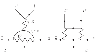
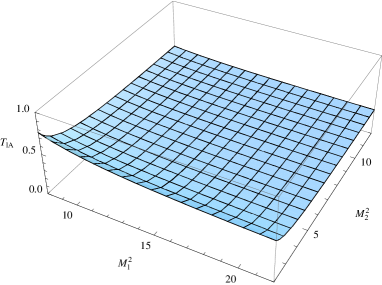
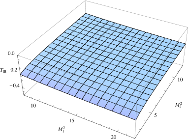 (b)
(b)
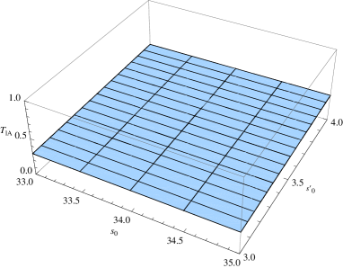 (c)
(c) 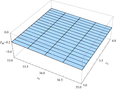 (d)
(d)
 (b)
(b)
 (b)
(b)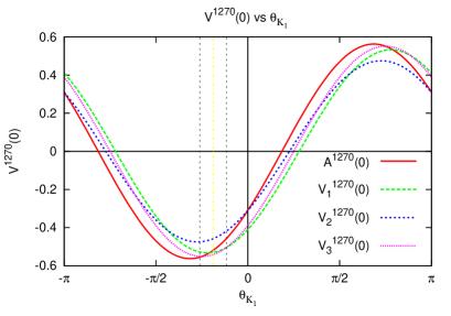
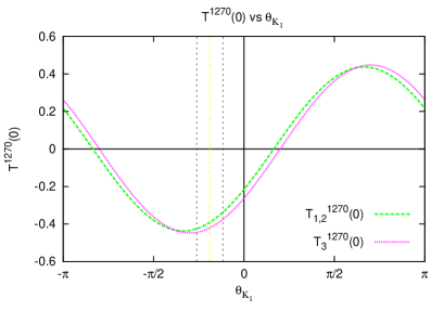 (b)
(b)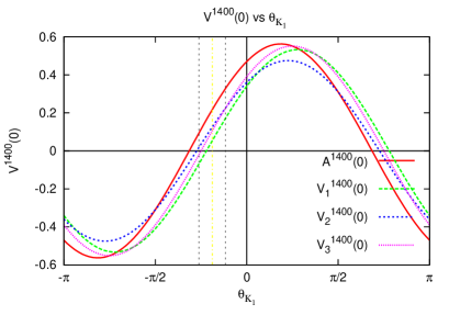
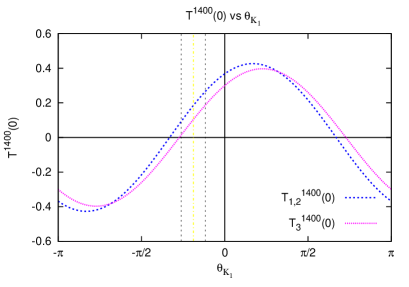 (b)
(b)