Status of dynamical ensemble generation

Abstract:

I give an overview of current and future plans of dynamical QCD ensemble generation activities. A comparison of simulation cost between different discretizations is made. Recent developments in techniques and algorithms used in QCD dynamical simulations, especially mass reweighting, are also discussed.

1 Introduction

Recently there has been a remarkable progress in reaching continuum limit via Lattice QCD, made possible by better simulation algorithms and better lattice discretizations to suppress lattice spacing errors in moderate lattice spacings, in addition to steady advances in computing hardware. In many ways, it is more than just a rhetoric to say we are at the cusp of generating realistic lattice QCD configurations.

Since an extensive review of systematic errors, theoretical and practical issues of each lattice discretization schemes was given at the last year’s conference [1], here I will focus more on a survey of ongoing lattice ensemble activities and technical details from different groups presented at the conference and updates since the last year. More comprehensive review of physical quantities from these lattices will be made elsewhere, for example in [2, 3, 4, 5]. Also, a brief and incomplete review of recent progress and trends in dynamical simulation algorithms is given with more details on mass reweighting technique.

It should be noted that while the list of dynamical lattice QCD ensemble generation activities presented here is extensive, it is limited to only zero temperature ($T\geq L$) and ”QCD-like” ensemble simulations, with 2 light quarks. There are significant amount of ensemble generation activities for QCD thermodynamics studies and beyond the standard model studies, especially in anticipation of upcoming results from Large Hadron Collider(LHC). These topics are covered in [6] and [7] respectively.

The organization is as follows. Section 2 gives descriptions and summaries of ongoing ensemble generating activities. A comparison of simulation cost for various lattice discretizations is given in section 3. Section 4 summarizes available measurements of autocorrelations, especially topological charge. Summary of advances in simulation algorithms and techniques is given in section 5.

2 Ensembles

2.1 Domain Wall Fermion(DWF)

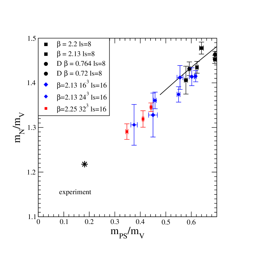
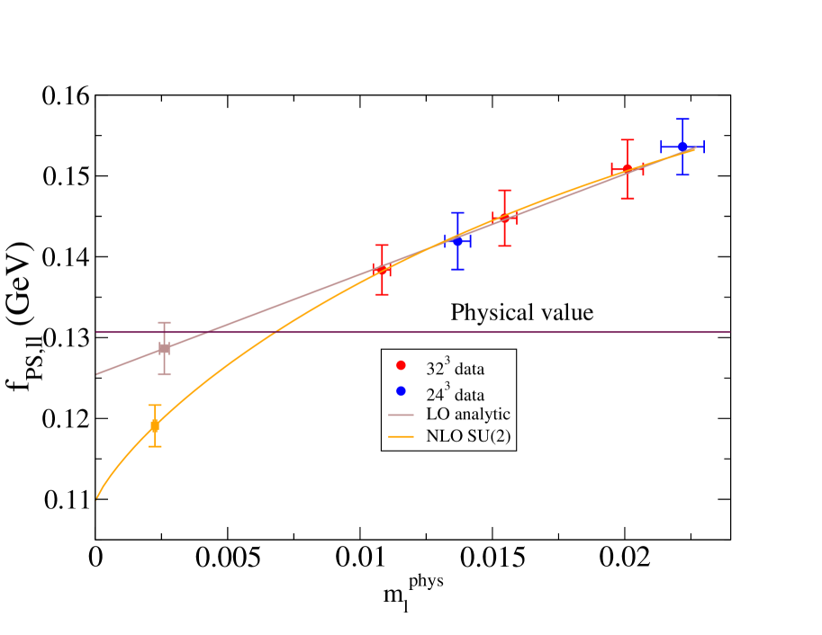
Figure 1: Edinburgh plot for dynamical DWF lattices, from[14].

Figure 2: Pseudoscalar decay constant($f_{\pi}$) with $m_{sea}=m_{val}$ for $24^{3}$ and $32^{3}$ DWF lattices, from[15].

RBC/UKQCD collaborations have been generating $N_{f}=2+1$ DWF configurations [8, 9, 10] using DWF formalism from [11] and Iwasaki gauge action[12] which gives a good balance between preservation of chiral symmetry and practicality for the lattice spacings studied so far. Iwasaki action was chosen instead of DBW2 action [13], which was used for previous DWF studies, to ensure sufficient decorrelation in topological charge.

A recent deployment of IBM BG/P machines at Argonne Leadership Computing Facility(ALCF) made the ensembles at the second lattice spacing much earlier than initially anticipated. Currently ensembles in 2 lattice spacings are available:

• $\beta=2.13,a\sim 0.121\mbox{fm},16^{3}\times 32\times 16,m_{\pi}\sim 400,526,627$ Mev

• $\beta=2.13,a\sim 0.114\mbox{fm},~{}24^{3}\times 64\times 16$, $m^{\bar{MS}}_{res}\sim$ 8.5 Mev, $m_{\pi}\sim$ 328, 417 Mev

• $\beta=2.25,a\sim 0.084\mbox{fm},~{}32^{4}\times 64\times 16$, $m^{\bar{MS}}_{res}\sim$ 2.45Mev, $m_{\pi}\sim$ 295, 350, 397 Mev

Figures 2 and 2 Shows the scaling behavior between DWF ensembles with 2 different lattice spacings. The quantities measured within the range of sea quark mass shows the scaling violation is within 2%. This allows fitting both ensembles to NLO SU(2) ChPT in $a^{2}$ and $m_{l}$, where only leading order(LO) ChPT low energy constants (LEC’s) have $a$ dependence. Reweighting in dynamical strange quark mass (section 5.1.1) and interpolation in valence mass is used to reach the physical strange quark mass point. Numbers in physical units for the last 2 sets of ensembles are from this SU(2) ChPT global fit using both ensembles. Details of the fitting procedure and the results for pseudoscalar meson and decay constants is reported in [16]. $B_{K}$ and detailed scaling study is reported in [15]. Results on hadron masses are in [14].

2.2 DWF with Auxiliary Determinant (Modified Gap DWF)

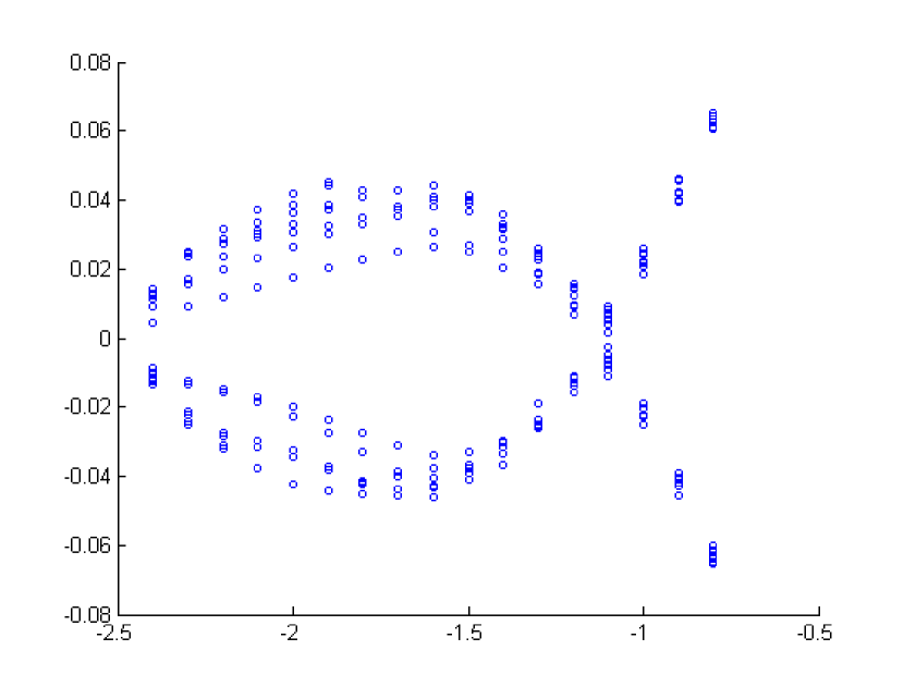
Figure 3: Time history for $\beta=1.75,m_{l}=0.042,32^{3}\times 64\times 32$ ensemble

Figure 4: Eigenvalue flow diagram for a $\beta=1.75,16^{3}\times 8\times 32$ lattice

Lattice dislocations which induce residual chiral symmetry breaking in DWF is currently the biggest obstacle for DWF and overlap fermions at larger lattice spacings. ($a\geq 0.1$ fm). Hence, controlling residual mass at these lattice spacings is crucial for DWF studies of quantities which requires large lattice volume, such as QCD thermodynamics, nucleon matrix elements, weak matrix elements via direct studies of $K\rightarrow\pi\pi$ process on the lattice.

Various approaches have been used to suppress dislocations in the past. Different gauge actions such as DBW2 action[13] have shown to suppress dislocations successfully, but at the expense of suppression of topology tunneling at smaller lattice spacings. Alternatively, additional fermion action can be used to suppress dislocations, as they are related to near zero modes of Wilson Dirac operators. This idea was first introduced in [17] and later used in dynamical overlap simulation by JLQCD collaboration[18], where a ratio of Wilson fermion determinants were used instead. It should be noted that while formally fermions are added, these are not related to physical quarks and this is effectively just changing gauge action after they are integrated out.

For the lattice spacings currently being investigated, determinants used in either [17] or [18] appear to suppresses the topology tunnelling too strongly. To circumvent this, a small imaginary mass is also added to the numerator to ensure the zero eigenvalues are not completely suppressed.

Supression factor from these additional terms is given by

$$\mathcal{W}(M_{5},\epsilon_{f},\epsilon_{b})=\frac{\det\left[D_{W}(-M_{5}+\imath\epsilon_{f}\gamma^{5})^{\dagger}D_{W}(-M_{5}+\imath\epsilon_{f}\gamma^{5})\right]}{\det\left[D_{W}(-M_{5}+\imath\epsilon_{b}\gamma^{5})^{\dagger}D_{W}(-M_{5}+\imath\epsilon_{b}\gamma^{5})\right]}$$

$$=\frac{\det\left[H_{W}(-M_{5})^{\dagger}H_{W}(-M_{5})+\epsilon_{f}^{2}\right]}{\det\left[H_{W}(-M_{5})^{\dagger}H_{W}(-M_{5})+\epsilon_{b}^{2}\right]}=\prod_{i}\frac{\lambda^{2}_{i}+\epsilon^{2}_{f}}{\lambda^{2}_{i}+\epsilon^{2}_{b}}$$ (1)

Where $\lambda_{i}$ are eigenvalues of Hermitian Wilson dirac operator with mass $-M_{5},H_{W}(-M_{5})=\gamma_{5}D_{W}(-M_{5})$. Eq. (1) gives $\sim 1$ for $\lambda_{i}\gg\epsilon_{b},\epsilon_{f}$, while $\sim\epsilon^{2}_{f}/\epsilon^{2}_{b}$ for $\lambda_{i}\ll\epsilon_{f},\epsilon_{b}$. $\epsilon_{f}=0$ corresponds to what is used in [18] and only numerator with $\epsilon_{f}=0$ was used in [17].

Aux. Det. $\beta=1.75,a\sim 1.4\mbox{Gev},\epsilon_{f}/\epsilon_{b}=0.02/0.5,am_{res}\sim 0.0019$
$L/a$	$m_{s}a$	$m_{l}a$	$L(fm)$	$m_{PS}$(Mev)	$\tau$(MD)	Accept.
$32^{3}\times 64\times 32$	0.045	0.0042	$\sim$ 4.5	$\sim 250$	$\sim$ 1200	$\sim$ 70%
$32^{3}\times 64\times 32$	0.045	0.001	$\sim$ 4.5	$\sim 200$	$\sim$ 250	$\sim$ 70 %

Table 1: List of ongoing ensemble generation using DWF with Eq. (1).

Table 1 shows the ongoing DWF simulations with the auxiliary determinant. Although it turned out it is necessary to use a rather large $\epsilon_{b}$ to make enough suppression of the residual mass, which causes the shifts in gauge coupling $\beta$, a factor of 5-7 decrease in residual mass was observed after the scales are matched by locating transition temperature [19].

Figure 4 shows the topological charge evolution of these ensembles and Wilson Dirac operator eigenvalue flow diagram for an ensemble with same lattice spacing and smaller volume, which suggests the topology is being sampled well while dislocations which causes the small eigenvalues near $-M_{5}=1.8$ are suppressed as intended.

Preliminary results form $m_{\pi}\sim 250$Mev ensembles suggests that the scaling error between $a\sim 0.14$fm AuxDet ensembles and existing DWF ensembles is at a few percent level, and it is possible to fit DWF ensembles with and without the auxiliary determinant in a fashion in [16], by allowing different $a^{2}$ dependence to LO LEC’s in the ChPT fitting. Result of this analysis will be forthcoming.

2.3 $a^{2}$, tadpole improved staggered action (Asqtad)

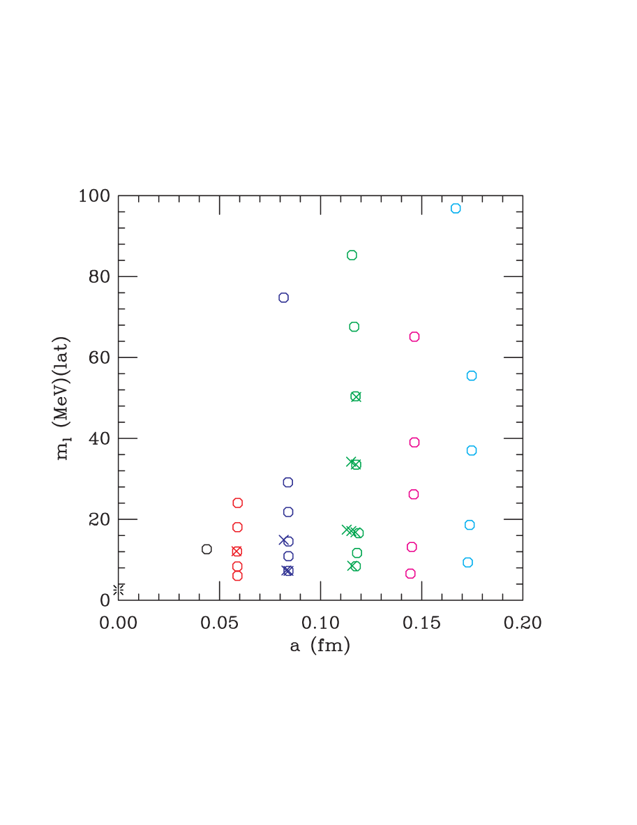
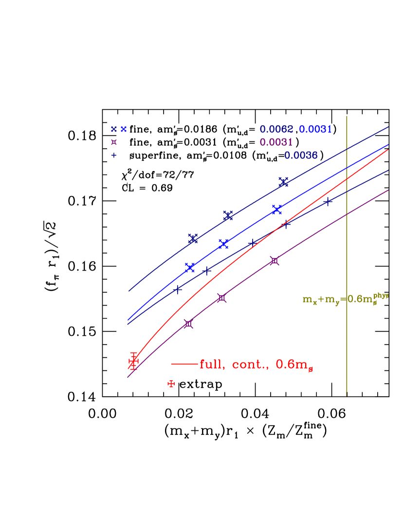
Figure 5: Lattice spacing and light quark masses of available $N_{f}=2+1$ dynamical Asqtad ensembles, from [20].

Figure 6: SU(3) ChPT fit to $f_{\pi}$ from [21]. Red line shows the continuum extrapolation with $m_{s}\sim 0.6m_{s}^{phys}$.

MILC collaboration has been generating $N_{f}=2+1$ dynamical ensembles with improved staggered fermion action(Asqtad)[22], designed to suppress taste symmetry violation present in staggered fermions, with multiple lattice spacings and quark masses. An extensive review of ensembles and physics results is given in [20].

As shown in figure 6, most of the simulation is done $0.4\geq m_{l}/m_{s}\geq$0.1, which gives $m_{\pi}\geq 220$ Mev, at multiple lattice spacings, $a\sim$ 0.15 (usually referred as ”extra-coarse”), 0.12 (coarse), 0.09 (fine), 0.06 (superfine), 0.045 (ultrafine) fm. In addition to these, there are ensembles generated at $m_{s}$ near 60% of physical strange quark mass, to aid SU(3) ChPT studies. Most recent continuum extrapolation of Sommer scale $r_{1}$, set by $f_{K}$, gives 0.3117 fm [21]. Typically staggered chiral perturbation theory[23, 24] is used for continuum extrapolations. An update of SU(3) ChPT fitting results are reported in [21].

It should also be noted that MILC ensembles have been extensively used for various mixed action studies, for example [25], where valence quarks with different discretizations are used, due to early availability of ensembles with multiple lattice spacings and quark masses. For these studies, the effects of taste symmetry breaking also has to be accounted for and this is typically done via mixed action chiral perturbation theories such as[26].

2.4 Highly Improved Staggered Quarks (HISQ)

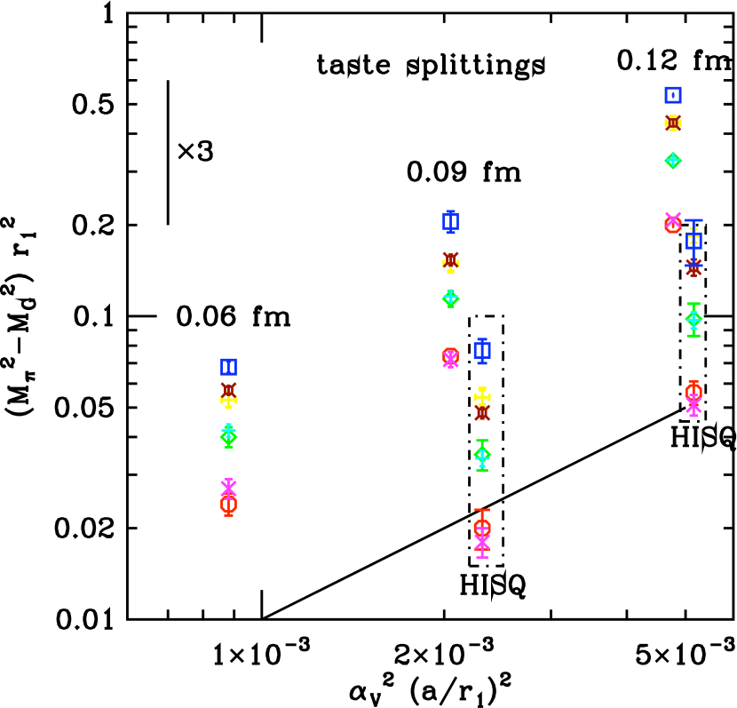
Figure 7: Taste splitting of Asqtad and HISQ action, measured by the difference of squared pseudoscalar meson masses with different tastes[28]. $M_{I}$ and $M_{G}$ is the mass of taste singlet and Goldstone pseudoscalar respectively.

Figure 8: Scaling plot of nucleon mass for Asqtad and HISQ actions[28].

HISQ action [27] is a staggered fermion action, improved further from Asqtad action by introducing additional Fat-7 smearing followed by projection to U(3) using Cayley-Hamilton theorem, used also in [29, 30], before combined in a similar fashion to Asqtad action.

Preliminary studies of dynamical ensembles generated with HISQ action indicates that while it is about 2 times more expensive per MD units compared to those of Asqtad actions at the similar lattice spacing, the mass splitting between pseudoscalar mesons with different tastes are reduced by a factor of $2.5\sim 3$ (Fig. 8).

While the U(3) projection after additional smearing have shown to be effective in suppressing taste symmetry breakings, this also causes the fermion force for MD steps to be large when the smeared link happens to have a small eigenvalue, resulting in low acceptance. These difficulty is avoided by replacing $Q^{-1/2}$ with $(Q+\delta I)^{-1/2}(\delta\sim 5\times 10^{-5})$ during moleculardynamics (MD) steps, where $Q$ is a smeared link to be projected to U(3). While this effectively changes the hamiltonian for MD step, Metropolis step after each trajectory corrects for the discrepancy. Also, dynamical charm quark can be included with $O((am_{c})^{4}))$ errors removed, but the coefficient for a straight 3-link term (Naik term) should be set different for different quarks.

Preliminary studies with HISQ actions for both thermodynamic studies ($N_{f}=2+1$) [31] and zero temperature studies with dynamical charm quark ($N_{f}=2+1+1$)[28] are reported at the conference.

2.5 $\mathcal{O}(a)$ improved Wilson (Clover) action

There are ensemble generation activities by several collaborations using Clover actions: Budapest-Marseilles-Wuppertal(BMW) collaboration, PACS-CS collaboration, QCDSF collaboration and Coordinated Lattice Simulations(CLS) collaboration. All activities are aimed at generating ensembles with the pion mass close or at the physical value. The main features of simulations are summarized in table 2.

Collaboration	BMW	PACS-CS	QCDSF		CLS
$N_{f}$	2+1	2+1	2	2+1(SLiNC)	2
Gauge action	Tree Symanzik	Iwasaki	Wilson	Tree Symanzik	Wilson
$c_{sw}$	Tree level	NP	NP		NP
Smearing	Stout			Stout
Algorithm	(R)HMC	DDHMC	(R)HMC		DDHMC
		+PHMC			+deflation
$a$(fm)	0.065-0.125	0.09	0.072-0.09	$\sim$0.08	0.04-0.08
$m_{\pi}$(Mev)	$>\sim$ 190	156-702	140 - 1010		360 - 520
This conference	[32]	[33]	[34]	[35]	[36]

Table 2: Summary of dynamical Clover ensemble generation activities.

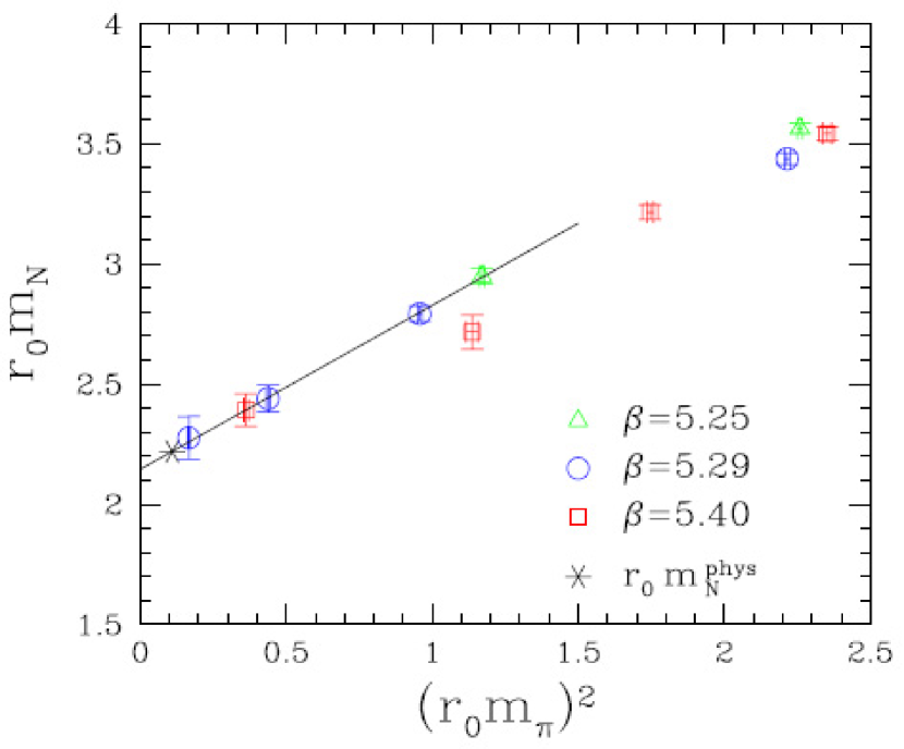
Figure 9: Deviation of hadron masses from physical values, normalized by $m_{\Omega}$, from [33].

Figure 10: Nucleon mass versus $m_{\pi}^{2}$ from QCDSF $N_{F}=2$ ensembles. $M_{N}\sim m_{\pi}^{2}$ behavior is observed. $r_{0}=0.467$ fm is used.

While nonpurtabatively determined $c_{sw}$ is used for most of simulations, ensembles generated by BMW collaboration uses tree level value, but instead rely on up to six levels of stout smearing[29] to suppress lattice discretization errors. The main results from these ensembles were reported in[37, 38, 39] and update of $f_{K}/f_{\pi}$ is given in [32].

PACS-CS[40, 41] has applied mass reweighting technique(section 5.1) to tune both light and strange dynamical masses to reach physical point for figure 10. Currently available configurations have a physical size $L\sim$ 3 fm, $m_{\pi}L\sim 2.2$. Simulation with $L\sim$6 fm is under way.

QCDSF collaboration has generated extensive $N_{f}=2$ ensembles and the results for hadron masses from those configurations are given in [34]. They are also working on $N_{f}=2+1$ ensembles using stout smearing and nonperturbative $c_{sw}$, called SLiNC action. A preliminary study for tuning quark masses to physical point is described in [35]. $r_{0}=0.5$ fm is used to set the scale.

CLS collaboration[42] aims to generate Clover ensembles in a wide range of lattice spacings, quark masses and lattice volumes using deflation accelerated DD-HMC[43]. Preliminary results are reported in [36].

2.6 Twisted mass Wilson(tmWilson)

European Twisted Mass Collaboration(ETMC) has been generating both $N_{f}=2$ and $N_{f}=2+1+1$ dynamical tmWilson ensembles [44, 45] with maximal twist. $N_{f}=2$ ensembles are generated with tree-level Symanzik gauge action, 0.053 fm $<a<0.1$ fm, 280 Mev $<m_{\pi}<$ 650Mev and 2.0 fm$<L<2.5$fm.

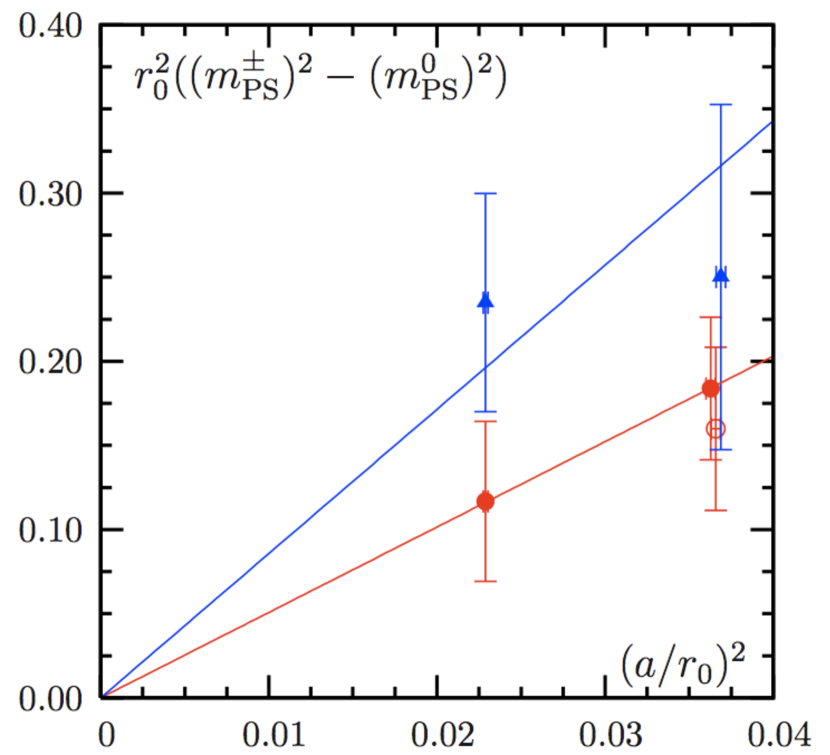
Figure 11: $(m_{\pi}^{\pm})^{2}-(m_{\pi}^{0})^{2}$ vs. $a^{2}$ for tmWilson $N_{f}=2$ ensembles.

Figure 12: $f_{\pi}$ vs $m_{\pi}$ for tmWilson $N_{f}=2$ and 2+1+1 ensembles[46].

A more detailed scaling study on $N_{f}=2$ ensembles shows a good scaling between ensembles with 4 different lattice spacings for many quantities. An exception to this is the mass splitting between charged and neutral pseudoscalar mesons from the breaking of isospin symmetry at nonzero lattice spacing. Figure 12 shows while the behavior is consistent with $O(a^{2})$ effect, it still is significant in the lattice spacings studied. This may be understood via a Symanzik-type analysis[47]. More details of $N_{f}=2$ ensembles is reported in [48].

$N_{f}=2+1+1$ ensembles are generated with Iwasaki gauge action, at $a\sim 0.078,0.086$fm, 280Mev, $<m_{\pi}<$ 500Mev, $L<\sim 2.8$fm. Polynomial HMC(PHMC)[49] is used for the fermion simulation. Twist parameters for heavy quarks, $\mu_{\sigma}$ and $\mu_{\delta}$, are fixed by tuning to physical values of $K$ and $D$ mass while keeping $m_{PCAC,l}$ close to zero. This is done without calculating all the possible excited states such as $K+n\times\pi$ between K and D meson masses by assuming some properties about our trial states and the corresponding correlation matrices. it turned out $\mu_{\delta}$ was slightly underestimated for some of the ensembles. This is planned to be adjusted by reweighting[50]. More details of $N_{f}=2+1+1$ ensembles is reported in [46].

In addition to this, $N_{f}=4$ ensemble is being generated for nonperturbative renormalization with RI-MOM scheme[51].

2.7 Anisotropic Clover

Hadron Spectrum Collaboration(HSC) has been generating $N_{f}=2+1$ anisotropic clover configurations at $a_{s}=0.125~{}\mbox{fm},\xi=a_{s}/a_{t}=3.5,a_{t}\sim 5.6$ Gev, $L=3\sim 4$ fm, $m_{\pi}=$ 230, 360 Mev to study various quantities such as resonance spectroscopy and nuclear forces. Stout smearing is used on spatial links only to suppress discretization errors further while preserving locality of transfer matrix. Strange quark is tuned to keep $s_{\Omega}=9(2m_{K}^{2}-m_{\pi}^{2})/(2m_{\Omega})^{2}$ constant while approaching continuum, as shown in figure 14. More details of algorithm and mass tuning are given in [52, 53]. Results using these ensembles on excited nucleon spectroscopy [54], $\pi\pi$ states using distilled quark propagators [55], multi-hadron systems[56] and cascade baryons[57] are reported at the conference.

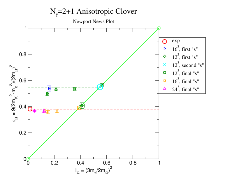
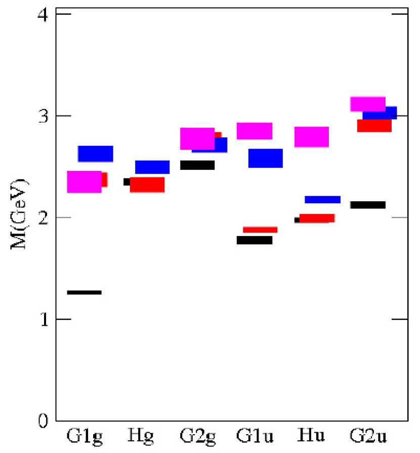
Figure 13: $s_{\Omega}=9(2m_{K}^{2}-m_{\pi}^{2})/(2m_{\Omega})^{2}$ vs. $l_{\Omega}(3m_{\pi}/3m_{\Omega})^{2}$ (Newport News) plot.

Figure 14: Preliminary results for resonance spectrum from $N_{f}=2+1,m_{\pi}=380$ Mev, $16^{3}\times 128$ anisotropic clover ensembles[54].

2.8 Overlap and Optimal DWF

JLQCD and TWQCD collaboration has been generating $N_{f}=2$ [18] and $N_{f}=2+1$ overlap ensembles with $a\sim 0.1-0.12$fm, $L\leq 2$ fm. Recent results are covered separately in [58, 59].

Also, TWQCD collaboration has started generating $n_{f}=$ 2 and 2+1 ensembles using optimal domain wall fermion[60] with $a^{-1}>\sim$ 1.6 Gev, $L=2\sim 3$ fm. These simulations are performed with CUDA-written codes on Nvidia GPGPU (Nvidia Tesla S1070, 46 Nvidia GTX285/280). More details of TWQCD activities can be found in [61].

2.9 Chirally Improved fermion(CI)

Bern-Graz-Regensburg(BGR) collaboration has started generating $N_{f}=2$ configurations using CI action[62], a 4 dimensional action with links of length up to 4, tuned to satisfy Ginsparg-Wilson relation approximately. Stout smearing is used to suppress discretization error further along with Lüscher-Weisz Gauge action. Figure 15 shows collection of links conneced to the point at the center in CI action. Currently generated ensembles have $N_{f}=2,16^{3}\times 32,\sim 2.4$ fm, 318 $<m_{\pi}<526$ Mev, $m_{AWI}=15\sim 42$ Mev. This gives a significantly different action to be used for studies of excited states to anisotropic Clover in section 2.7. Preliminary results for excited hadron spectrum is reported in [63].

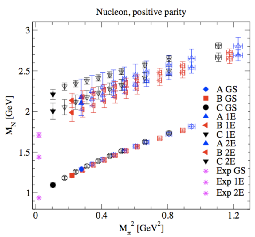
Figure 15: Illustration of paths and Nucleon excited states from CI action, from[63].

3 Simulation cost

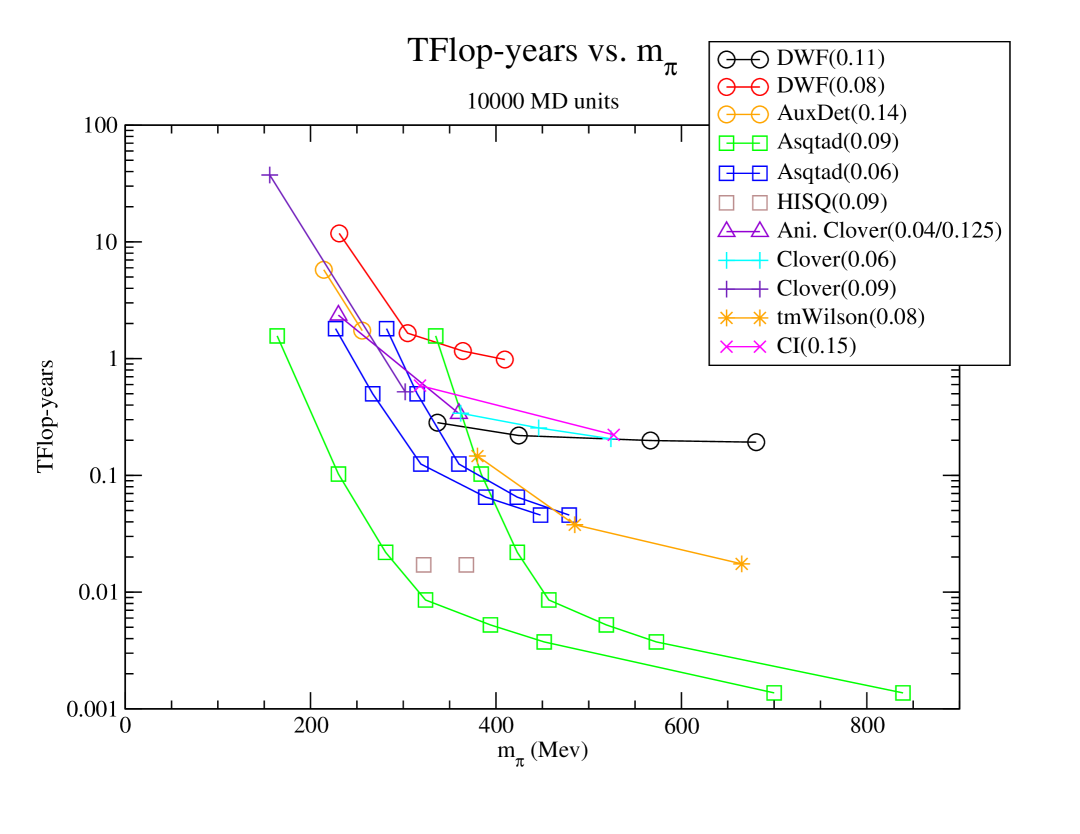
Figure 16: Total number of TFlop-years needed for $10^{4}$ MD units versus $m_{\pi}$(Mev) at physical volume $L^{3}\times T$ satisfying eq. (2), scaled from numbers for existing ensembles by (cost) $\sim V^{5/4}$. 2 separate lines with same colors for Asqtad and HISQ ensembles represent the lightest(Goldstone) and the heaviest(taste singlet) pseudoscalar masses. Numbers for Asqtad and HISQ simulations are calculated from eq. (4). tmWilson(0.08) is from ETMC[64]. Clover(0.09) is from PACS-CS[40]. Clover(0.006) is from CLS[68].

As listed in the section above, there are many ongoing dynamical ensemble generation activities with different discretizations. This is not just because of increasing availabilty of computing resources, but rather the reflection of the fact that different actions have different lattice spacing error for different quantities at same lattice spacings, and the recent progress in ensemble generation algorithms makes ensemble generation relatively cheaper compared to the valence propagator generation, either with the same or different discretization, and relying on one discretization method to get every physical quantities of interest may not turn out to be the most cost-efficient approach. This also suggest a comparison of different actions at the same lattice spacing is not necessarily a fair one.

Having said that, it is still useful to have some idea on how expensive each action is at a given lattice spacing and quark mass. Here such a comparison is made by estimating the number of flops to generate the same number of MD units for each action from available performance data. Recent studies indicate it is necessary to keep physical volumes to be larger than previously deemed sufficient to control finite size effect, so for a given lattice spacing $a$ and pseudoscalar meson mass $m_{\pi}$ for each existing ensembles, the number of flops are scaled to a volume $L^{3}\times T$ which satisfies

$$L=\mbox{Max}(4/m_{\pi},\quad\ 2.5\mbox{fm}),\quad\ T=2L.$$ (2)

First, available cost formulas in TFlop-years to generate 10000 MD units or 100 statistically independent configurations are given below. here $L,T,a$ are in fm and $m_{\pi},m_{K},m_{l},m_{s}$ are in Mev.

$$Cost[DWF]\cite[cite]{[\@@bibref{}{Christ:2006zz}{}{}]}:\sim\left(\frac{L^{3}\times T}{a^{4}}\right)^{5/4}\left(\frac{1}{m_{\pi}a}\right)\left[C_{0}+C_{1}\frac{1}{m_{K}^{2}a}+C_{2}\left(\frac{a}{m_{\pi}}\right)^{2}\right]$$ (3)

$$Cost[Asqtad]\cite[cite]{[\@@bibref{}{MILC_cost}{}{}]}\sim\frac{2.9}{64^{3}\times 144}\left(\frac{L^{3}\times T}{a^{4}}\right)^{5/4}\frac{0.1}{m_{l}/m_{s}}\frac{0.06}{a}\left(0.5+0.5\frac{0.1}{m_{l}/m_{s}}\frac{0.06}{a}\right)$$ (4)

$$Cost[HISQ]\sim 2\times Cost[Asqtad]$$

$$Cost[Clover(DD-HMC)]\cite[cite]{[\@@bibref{}{DelDebbio:2006cn}{}{}]}\sim 0.05\times\left(\frac{20}{\bar{m_{l}}}\right)\left(\frac{L}{3}\right)^{5}\left(\frac{0.1}{a}\right)^{6}$$ (5)

While these formulas show different dependencies in $a$ or $m_{q}(m_{\pi})$, they all have the same dependence in volume, (cost) $\sim V^{5/4}$, which is all we need for the comparison outlined above.

Figure 16 shows the number of total TFlop-years needed to generate 10000 MD units of gauge configurations with the lattice spacings and pseudoscalar masses of existing ensembles, with the volume scaled to satisfy eq.(2). While it should be noted that there are differences in precisely how flops are counted for each ensembles which results in some uncertainties in comparing different ensembles. However, it does appear that the difference in total cost between different actions tends to get smaller as the quark mass approaches the physical point. This is presumably because the low, physical eigenmodes of Dirac operators increasingly dominate the cost near the chiral limit, while simply the number of degrees of freedom per sites counts more for simulations at heavier masses.

Still, the cost is a rapidly changing function of the lattice spacing and any real cost comparison should be done not only with these numbers, but in combination with how small lattice spacing error is required for the quantities one aims to study with each action.

4 Autocorrelation

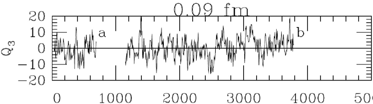
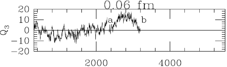
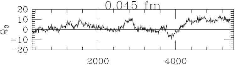
Figure 17: Time history of global topological charge for Asqtad ensembles at $m_{l}/m_{s}=0.2~{}(m_{\pi}\sim$ 320 Mev)[72]. The lattice spacings are indicated above each graph.

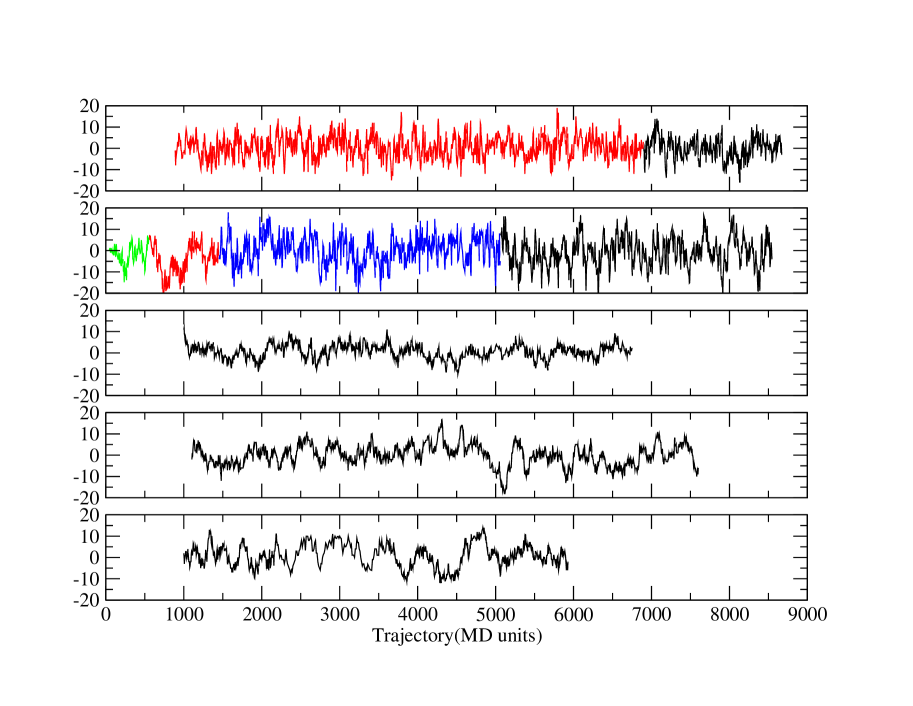
Figure 18: Time history of topological charge for DWF ensembles. The ensembles are as follows from the top: ($a\sim 0.11\mbox{fm}:am_{l}=0.005,0.01),(a\sim 0.08:am_{l}=0.004,0.006,0.008)$.

For obvious reasons, autocorrelations within ensembles is a significant factor in what the real cost of generating a number of independent configurations is. Unfortunately, in practice this is not necessarily something one can measure easily, even after ensemble generation is nominally finished, as it can and does vary greatly between different quantities.

While all the ensembles reported here have reasonable ($<100$ MD units) autocorrelation time for quantities such as plaquette, meson propagators and number of CG iterations, many of them only a few MD units, a significant slowdown of change in global topological charge was observed in ensembles with relatively smaller lattice spacings. Time evolution of topological charge in both asqtad and DWF ensembles are shown in Figures 17 and 18. A similar behavior was also observed in clover action simulations with DD-HMC[69]. While the global topological charge itself may or may not be relevant in physics as long as the physical volume is large enough, it still is a sign of failures of evolution algorithms currently in use to ensure ergodicity of each ensemble.

While these results are still preliminary and requires more careful studies, if not longer ensembles, it would be crucial to check this for any ensembles, especially ensembles with smaller lattice spacings, since these ensembles are designed to have systematic errors small enough for precision studies, and long autocorrelations affect the cost of generating independent configurations to control the statistical errors significantly, or introduce systematic errors from failing to sample all the topological sectors.

This also presents a potential problem in relying on staying on the same lattice discretization and increasingly smaller lattice spacing, made possible by increasing computing resources, to control the discretization error. This might make it preferable to make better use of increasing computing resources by keeping the lattice spacing moderate and try more improved actions with smaller lattice spacing error, instead of continuing more conventional actions at smaller lattice spacing. Unfortunately, currently this approach - comparing different discretizations - is hampered substantially by the lack of a quantity easily measurable with known and accurate physical value to fix the lattice spacing, as shown by different values of $r_{0,1}$’s used or measured for different discretizations in section 2.

This is not to say this problem cannot be circumvented by algorithmic development. The fact that the increase in autocorrelation is largely independent of the quark mass, choice of discretization and simulation algorithms[69] suggests the gauge action is the culprit, and techniques for more aggressive decorrelation while keeping the action the same, such as Noisy Monte Carlo[70], or even drastically different ideas such as [71], could turn out to be effective.

5 Algorithms and techniques

In the last several years, there have been much progress in fermion simulation algorithm. Improvements such as Rational Hybrid Monte Carlo[73], higher order integrators, particularly Omelyan[74, 75], multiscale integrators and mass preconditioning[76] achieved almost ubiquitous usage, similar to what $\Phi$ and R algorithm[77] used to be. While these advances made details of fermion action unique for each simulation and made extensive tuning necessary, they also made, in combination with advances in hardware, the dynamical simulations with pion masses at or close physical value and made the cost of ensemble generation much less dominating compared to valence propagator generation needed for various analyses. This is certainly not to say we have exhausted the possibility of improvement. Algorithmic development such as force gradient integrator and better tuning via shadow hamiltonian[78, 79] suggests further reduction in cost of realistic QCD ensemble generation is possible.

Here some of more recent advances in algorithms are summarized, starting with mass reweighting technique, which has shown to be surprisingly useful.

5.1 Reweighting

The basic Idea of reweighting is well known. There are more than one Hamiltionians used in typical Monte Carlo simulations:

• Guiding Hamiltonian for Molecular Dynamics:
  $dU/dt_{MD}=-iHU,\quad\ d{\cal H}_{1}/dt_{MD}=0$ (As pointed out, for example in [78], MD integrators are not exact. Here ${\cal H}_{1}$ is the hamiltonian used to construct MD integrator, not the one actually being preserved by it .)

• Hamiltonian for Metropolis step :
  Acceptance = Min$\left(1,\exp\left[-({\cal H}_{2}({U}_{i+1})-{\cal H}_{2}({U}_{i}))\right]\right)$

• Hamiltonian for ensemble averaging

  $$<O>_{{\cal H}_{3}}=\frac{\int[dU]O(U)W(U)}{\int[dU]W(U)},\quad\ W(U)=\exp{\left[-({\cal H}_{3}(U)-{\cal H}_{2}(U))\right]}$$ (6)

Typically it is called ”reweighting” when ${\cal H}_{2}$ is intentionally set different from ${\cal H}_{3}$. In principle ${\cal H}_{1},{\cal H}_{2},{\cal H}_{3}$ can be all different and there are working examples, ranging from subtle ones such as using less precision and/or relaxed stopping condition for Hybrid Monte Carlo, to more explicit ones used to avoid singularities in HISQ action(section 2.4) where ${\cal H}_{1}\neq{\cal H}_{2}$, to many thermodynamic studies, to locate the phase transition temperature[80] or circumvent difficulties with finite density[81] where ${\cal H}_{2}\neq{\cal H}_{3}$.

However, ${\cal H}_{1,2,3}$ are extensive quantities (${\cal H}\propto V$) and conventional wisdom has been that it is hard to find ${\cal H}$’s which the acceptance/reweighting factor $e^{-\Delta{\cal H}}$ is close enough to 1 while it is different enough to give significant benefit for simulations with larger volumes. (For example, $32^{3}$ DWF simulations reported in section 2.1 has ${\cal H}$ on the order of $10^{8}$.)

However, recently some more working examples have been reported, such as reweighting of light quark [82, 83] and strang quark [84, 33] toward the physical point. While more aggressive reweighting such as those for light quark have potential to be more beneficial in the long run, the reweighting of strange quark mass in particualr has proved to be a cost effective way of eliminating one of the major sources of systematic error and provide an immediate benefit. A more detailed description of strange quark reweighting is given below.

5.1.1 Reweighting of dynamical strange quark

Due to the nonperturbative nature of QCD, lattice spacing of any lattice QCD simulation, with or without fermions, is not known a priori until it is measured on thermalized configurations.

Somewhat ironically, this has not posed problem for light quarks in practice as much, as typically multiple ensembles of different light quark masses are generated to do extrapolations to the chiral limit anyways, recent simulations near or at physical point notwithstanding. However, it is in principle possible and would be quite beneficial to simulate at the correct physical strange quark. Unfortunately, this is not the case and the dynamical strange quark is often different from physical value by up to 20%. Traditionally one of these approaches has been taken to address this problem:

• Generate multiple ensembles with different dynamical strange quark masses near physical value and use interpolation

• Using SU(3) ChPT to fit up to the strange quark.

• Do multiple parameter tuning runs in smaller volume before larger runs.

• Include the effect of discrepancy as a systematic error.

None of these approaches are particularly attractive and can be time consuming. It can save significant computing (and human) resources if this can be avoided.

It turned out the reweighting factor $W(U)$ (Eq.((6))) is often close to 1 even when strange quark mass is $10\sim 20\%$ different from the dynamical value, which makes the tuning of strange quark to the physical value via reweighting possible. This technique can also be used to calculate derivative with respect to the dynamical quark mass[85].

Reweighting factor for 1 flavor can be calculated as follows:

$$W([U],m_{s},m_{s}^{\prime})=\det\left(\frac{D^{\prime\dagger}D^{\prime}}{D^{\dagger}D}\right)^{1/2}=\mbox{det}(\Omega)^{-1/2},\Omega([U],m_{s},m_{s}^{\prime})=D^{\prime-1}DD^{\dagger}(D^{\prime\dagger})^{-1}$$

$$D=D([U],m_{l},m_{s}),D^{\prime}=([U],m_{l},m_{s}^{\prime})$$

$$W([U],m_{s},m_{s}^{\prime})=\frac{\int d\xi d\xi^{\dagger}e^{-\xi\dagger\sqrt{\Omega([U],m_{s},m_{s}^{\prime})}\xi}}{\int d\xi d\xi^{\dagger}e^{-\xi\dagger\xi}}=\left<e^{-\xi^{\dagger}(\sqrt{\Omega([U],m_{s},m_{s}^{\prime})}-1)\xi}\right>$$ (7)

where $\xi$ is a Gaussian random vector. $\sqrt{\Omega[U]}$ can be calculated using Rational approximation, similar to RHMC. Alternatively, the same reweighting factor can be calculated by

$$W([U],m_{s},m_{s}^{\prime})=\sqrt{\left<e^{-\xi^{\dagger}(\Omega[U]-1)\xi}\right>}$$ (8)

and it could be more efficient, as (8) can be calculated with just one inversion per random number. However, (8) is in principle a biased estimator and more accuracy than (7) is required for reweighting factors for each configurations to ensure the effect from inaccurate reweighting factor is under control, while (7) can be used without such requirement. Another scheme to use Taylor expansion to calculate square root is used in [33].

Due to the nature of (7) where each evaluation using random vector is exponentiated before average, it is essential to ensure $M=\sqrt{\Omega([U],m_{s},m_{s}^{\prime})}$ has only eigenvalues close to 1. In fact, it can be shown that the error in (7) diverges if $M$ has eigenvalues smaller than 1/2. Even when this is not the case, eigenvalues significantly away from 1 can make the reweighting factor converge very slowly with finite statistics. For mass reweighting, determinant breakup by intermediate masses[82]

$$W([U],m_{s},m_{s}^{\prime})=\Pi_{i=0}^{n_{m}-1}\left<e^{-\xi^{\dagger}(\sqrt{\Omega([U],m_{i},m_{i+1})}-1)\xi}\right>,$$

$$m_{s}=m_{0}<m_{1}<\cdots m_{n-1}<m_{n}=m_{s}^{\prime}\mbox{or vice versa}.$$

gives an additional benefit that the reweighting factors for the masses between $m_{s}$ and $m_{s}^{\prime}$ is automatically available. For other reweighting where this is not available, for example [86], Breakup using rational approximation, similar to ”root-N trick” in [73] is applicable.

Now, observables for $m_{s}^{\prime}$ is calculated from ensemble $[U_{i}]$ generated $m_{s}$ by

$$\left<O\right>(m_{s}^{\prime})=\frac{\Sigma_{i}O[U_{i}]W([U_{i}],m_{s},m_{s}^{\prime})}{\Sigma_{i}w[U_{i}]}$$ (9)

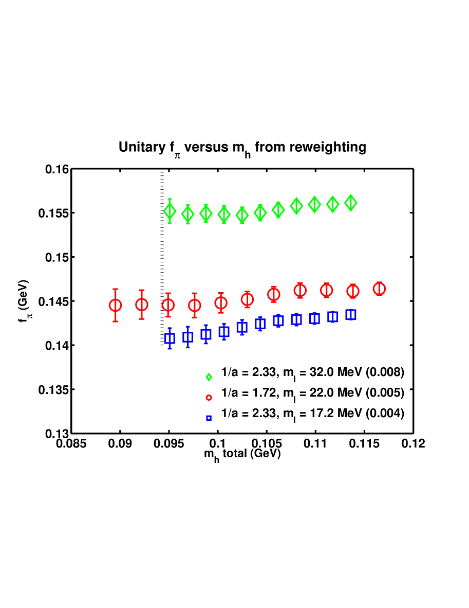
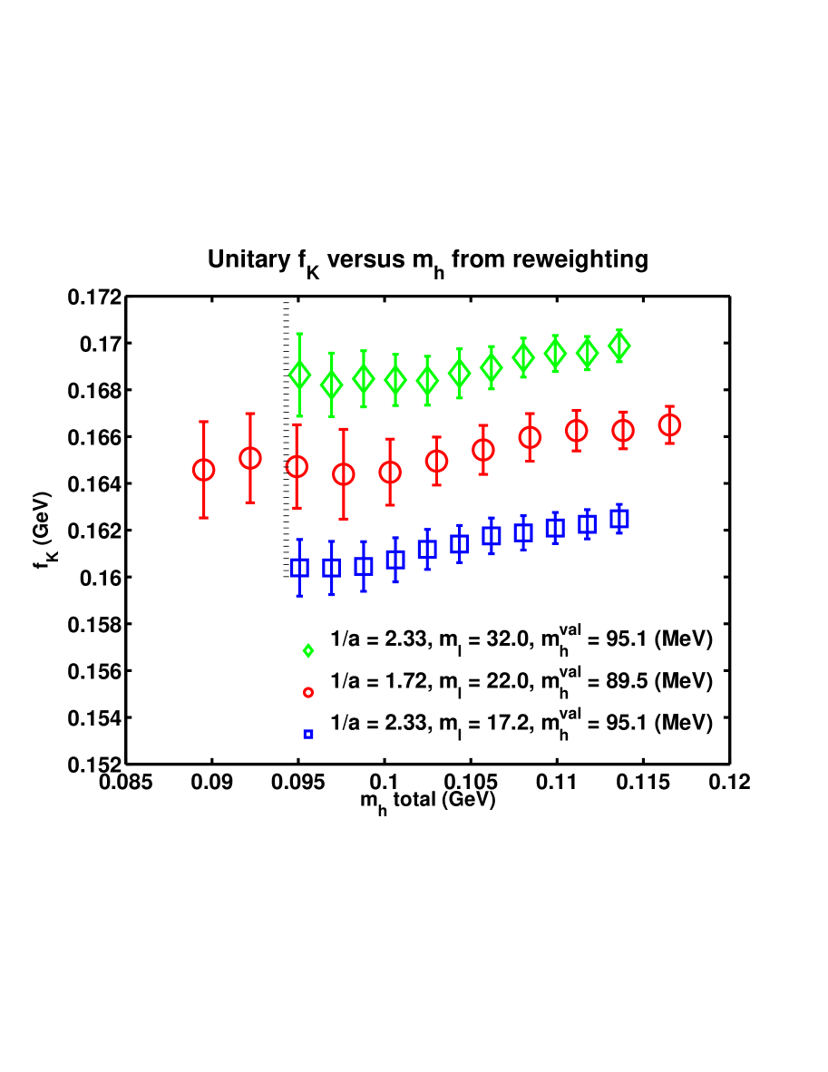
Figure 19: Reweighted $f_{\pi}$ and $f_{K}$ for $N_{f}=2+1$ DWF ensembles, from[16]. Broken vertical lines represent the physical strange quark mass and the rightmost points shows the original sea strange quark mass for each ensemble.

Figure 19 shows reweighted pseudoscalar decay constant of DWF ensemble in section 2.1. Even though only 4 random vectors per mass step is used to calculate reweighting factor for $a^{-1}\sim$ 2.33 Gev, $am_{l}=0.004$ ensemble, the reweighted values at $\sim 20\%$ smaller than $m_{s}$ has only slightly larger error than the error at $m_{s}$. As shown in section 2.5, PACS-CS collaborations has done both strange quark and light quark reweighting to reach physical point[33] and tuning of twist for the strange/charm quarks via reweighting is also being carried out by ETMC collaboration[50].

Given the success of mass reweighting, we can also think of other cases where reweighting can be helpful.

• ${\cal H}_{1}\neq{\cal H}_{2}$:

  • Using a relaxed approximation sign function during MD step of Overlap/Domain wall fermions, to avoid topology tunneling difficulties while preserving good chiral symmetry, this appears to be promising if the phase space where ${\cal H}_{1}\neq{\cal H}_{2}\geq 1$ is limited. One approach using DWF, namely reweighting to larger $L_{s}$ in DWF was explored in [86].

• ${\cal H}_{2}\neq{\cal H}_{3}$:

  • Apply reweighing to part or all of differences in action in mixed action studies. This would effectively trade systematic error with a statistical one.

  • Adding new terms to the action via reweighting, such as adding charm quarks to $N_{f}=2+1$ configurations or adding QED for studies of electromagnetic effects[87].

5.2 Nested/mixed precision solvers

Advent of many multicore chips, available currently or in the near future, present in principle significantly more computing power than currently available. However, this increase in computing power often comes without corresponding increase in bandwidth, both in memory and network. While it is not yet clearly shown that these architecture can achieve scalability suitable for large scale dynamical ensemble generations using conventional algorithms such as (R) HMC, or newer algorithms such as DD-HMC, it still is expected to provide competitive hardware platforms for propagator generation, where “embarrassingly parallel” - the local volume is chosen to be optimal for performance and run multiple jobs concurrently - approach is applicable.

The relative lack of memory bandwidth also pose problems for propagator generation even when it is possible to fit it on one node to circumvent the network bottleneck. One way to lessen the pressure on memory bandwidth is to use less precision arithmetic. While the relative difference in speed between single and double precision is significant for many existing platforms, until recently most frequently used approaches to take advantage of this was somewhat simple-minded, such as first solving in single precision and finish with double(less effective if small residual is required), MD in lower precision, Metropolis in double precision (if $\Delta H$ from precision loss is small, expected to scale poorly for larger volume), or even using single precision MD and skip Metropolis when the step size error is deemed smaller than other systematic errors.

Recently there have been rediscovery of algorithms, such as defect correction(used in [38]) and Reliable updates[88] for effective use of lower precision solvers for double precision inversions. Reliable update technique in particular has shown to be very effective in using single or half(16bit) precision, useful in GPGPU. More detailed description can be found in [90, 91]. In addition to this, there are other nested inversion algorithms such as Generalized Conjugate Residual(GCR), used with Domain decomposition[89] or inexact deflation[92]. A more extensive studies of these algorithms could allow much more effective inversion algorithms on existing and emerging architectures.

6 Conclusions

Recent advances in dynamical fermion simulation algorithms and continuing progress in hardware has enabled multiple collaborations to generate dynamical ensembles with different lattice discretizations, lattice spacings and dynamical quark masses. This is a striking departure from only a few years ago, when Asqtad configurations generated by the MILC collaboration were the only choice for continuum extrapolation with multiple lattice spacings and quark masses. Some of the ensembles are even being generated at or close to the physical pion mass. $N_{f}=2,2+1$ and 2+1+1 dynamical lattice QCD ensembles generation activities of various collaborations are summarized. It is shown that computing resources on the order of 10 to 100 TFlop-years, well within reach with technologies currently available, is enough to generate $N_{f}=2+1$ ensembles with $>100$ independent configurations at $m_{\pi}<200$ Mev and $m_{\pi}L>4$, barring the effect of autocorrelation observed by global topological charge.

A steep dependence of simulation cost on the lattice spacing and different scaling behavior of different actions, as well as the ambiguities in defining the lattice spacing itself, makes superficial comparisons between different actions not necessarily useful. Although it has become possible to use relatively inexpensive actions such as Wilson to generate ensembles very close to or at physical quark mass, the presence of significant autocorrelations observed by topological charge evolution at smaller lattice spacings ($a\leq 0.08$fm) should be better understood and circumvented to ensure usefulness of large scale ensembles. It is possible that multiple, more highly improved actions at a moderate lattice spacing is a better way to ensure that systematic errors are under control for all the quantities we are interested in studying. Presence of many ensemble generation activities is helpful in that respect.

Some of the recent progress in algorithms and techniques were also summarized. The mass reweighting technique, which turned out to be quite effective in eliminating one of the persistent source of systematic error is explained in more detail. Reweighting in general could alleviate the need to generate separate ensembles for slightly different parameters and/or actions, even for relatively large lattices.

Acknowledgments

I would like to thank the colleagues who sent previously unpublished materials before the conference for preparation of the talk, in particular A. Bazavov, T. Blum, T-W. Chiu, C. Detar, S. Gottlieb, G. Herdoiza, R. Horsley, B. Joo, Y. Kuramashi, C. B. Lang, R. D. Mawhinney, D. Palao, S. Reker, G. Schierholz and H. Wittig. I am also indebted to many RBC/UKQCD colleagues for many helpful discussions. The author was supported by the U.S. DOE under contract DE-AC02-98CH10886.

References

- [1] K. Jansen, “Lattice QCD: a critical status report,” PoS LATTICE2008 (2008) , arXiv:0810.5634 [hep-lat].
- [2] E. E. Scholz, “Light Hadron Masses and Decay Constants,” PoS LAT2009 (2009) 005, arXiv:0911.2191 [hep-lat].
- [3] C. Aubin, “Lattice studies of hadrons with heavy flavors,” PoS LAT2009 (2009) 007, arXiv:0909.2686 [hep-lat].
- [4] R. S. Van de Water, “The CKM matrix and flavor physics from lattice QCD,” PoS LAT2009 (2009) 014, arXiv:0911.3127 [hep-lat].
- [5] V. Lubicz, These proceedings, PoS(LAT2009)013.
- [6] M. Laine, “Finite-temperature QCD,” PoS LAT2009 (2009) 006, arXiv:0910.5168 [hep-lat].
- [7] E. Pallante, These proceedings, PoS(LAT2009)015.
- [8] RBC-UKQCD Collaboration, C. Allton et al., “Physical Results from 2+1 Flavor Domain Wall QCD and SU(2) Chiral Perturbation Theory,” Phys. Rev. D78 (2008) 114509, arXiv:0804.0473 [hep-lat].
- [9] RBC and UKQCD Collaboration, C. Allton et al., “2+1 flavor domain wall QCD on a (2 fm)3 lattice: light meson spectroscopy with Ls = 16,” Phys. Rev. D76 (2007) 014504, arXiv:hep-lat/0701013.
- [10] RBC Collaboration, D. J. Antonio et al., “Neutral kaon mixing from 2+1 flavor domain wall QCD,” Phys. Rev. Lett. 100 (2008) 032001, arXiv:hep-ph/0702042.
- [11] V. Furman and Y. Shamir, “Axial symmetries in lattice QCD with Kaplan fermions,” Nucl. Phys. B439 (1995) 54–78, arXiv:hep-lat/9405004.
- [12] Y. Iwasaki, “RENORMALIZATION GROUP ANALYSIS OF LATTICE THEORIES AND IMPROVED LATTICE ACTION. 2. FOUR-DIMENSIONAL NONABELIAN SU(N) GAUGE MODEL,”. UTHEP-118.
- [13] T. Takaishi, “Heavy quark potential and effective actions on blocked configurations,” Phys. Rev. D54 (1996) 1050–1053.
- [14] C. Maynard, These proceedings, PoS(LAT2009)091.
- [15] C. Kelly, P. A. Boyle, and C. T. Sachrajda, “Continuum results for light hadrons from 2+1 flavor DWF ensembles,” PoS LAT2009 (2009) 087, arXiv:0911.1309 [hep-lat].
- [16] R. Mawhinney, f. t. RBC, and U. Collaborations, “NLO and NNLO chiral fits for 2+1 flavor DWF ensembles,” PoS LAT2009 (2009) 081, arXiv:0910.3194 [hep-lat].
- [17] P. M. Vranas, “Gap domain wall fermions,” Phys. Rev. D74 (2006) 034512, arXiv:hep-lat/0606014.
- [18] JLQCD Collaboration, S. Aoki et al., “Two-flavor QCD simulation with exact chiral symmetry,” Phys. Rev. D78 (2008) 014508, arXiv:0803.3197 [hep-lat].
- [19] D. Renfrew, T. Blum, N. Christ, R. Mawhinney, and P. Vranas, “Controlling Residual Chiral Symmetry Breaking in Domain Wall Fermion Simulations,” PoS LATTICE2008 (2009) 048, arXiv:0902.2587 [hep-lat].
- [20] A. Bazavov et al., “Full nonperturbative QCD simulations with 2+1 flavors of improved staggered quarks,” arXiv:0903.3598 [hep-lat].
- [21] The MILC Collaboration, A. Bazavov et al., “Results from the MILC collaboration’s SU(3) chiral perturbation theory analysis,” PoS LAT2009 (2009) 079, arXiv:0910.3618 [hep-lat].
- [22] MILC Collaboration, K. Orginos, D. Toussaint, and R. L. Sugar, “Variants of fattening and flavor symmetry restoration,” Phys. Rev. D60 (1999) 054503, arXiv:hep-lat/9903032.
- [23] C. Aubin and C. Bernard, “Pion and Kaon masses in Staggered Chiral Perturbation Theory,” Phys. Rev. D68 (2003) 034014, arXiv:hep-lat/0304014.
- [24] C. Aubin and C. Bernard, “Pseudoscalar decay constants in staggered chiral perturbation theory,” Phys. Rev. D68 (2003) 074011, arXiv:hep-lat/0306026.
- [25] C. Aubin, J. Laiho, and R. S. Van de Water, “The neutral kaon mixing parameter from unquenched mixed-action lattice QCD,” arXiv:0905.3947 [hep-lat].
- [26] O. Bar, C. Bernard, G. Rupak, and N. Shoresh, “Chiral perturbation theory for staggered sea quarks and Ginsparg-Wilson valence quarks,” Phys. Rev. D72 (2005) 054502, arXiv:hep-lat/0503009.
- [27] HPQCD Collaboration, E. Follana et al., “Highly Improved Staggered Quarks on the Lattice, with Applications to Charm Physics,” Phys. Rev. D75 (2007) 054502, arXiv:hep-lat/0610092.
- [28] MILC Collaboration, . A. Bazavov et al., “Progress on four flavor QCD with the HISQ action,” PoS LAT2009 (2009) 123, arXiv:0911.0869 [hep-lat].
- [29] C. Morningstar and M. J. Peardon, “Analytic smearing of SU(3) link variables in lattice QCD,” Phys. Rev. D69 (2004) 054501, hep-lat/0311018.
- [30] A. Hasenfratz, R. Hoffmann, and S. Schaefer, “Hypercubic Smeared Links for Dynamical Fermions,” JHEP 05 (2007) 029, arXiv:hep-lat/0702028.
- [31] A. Bazavov, These proceedings, PoS(LAT2009)163.
- [32] A. Ramos , These proceedings, PoS(LAT2009)259.
- [33] PACS-CS Collaboration, S. Aoki et al., “Physical Point Simulation in 2+1 Flavor Lattice QCD,” arXiv:0911.2561 [hep-lat].
- [34] G. Schierholz , These proceedings, PoS(LAT2009)168.
- [35] W. Bietenholz et al., “Results from 2+1 flavours of SLiNC fermions,” PoS LAT2009 (2009) 102, arXiv:0910.2963 [hep-lat].
- [36] S. Capitani et al., “Mesonic and baryonic correlation functions at fine lattice spacings,” PoS LAT2009 (2009) 095, arXiv:0910.5578 [hep-lat].
- [37] S. Durr et al., “Ab-Initio Determination of Light Hadron Masses,” Science 322 (2008) 1224–1227, arXiv:0906.3599 [hep-lat].
- [38] S. Durr et al., “Scaling study of dynamical smeared-link clover fermions,” Phys. Rev. D79 (2009) 014501, arXiv:0802.2706 [hep-lat].
- [39] L. Lellouch, “Kaon physics: a lattice perspective,” PoS LATTICE2008 (2009) 015, arXiv:0902.4545 [hep-lat].
- [40] PACS-CS Collaboration, S. Aoki et al., “2+1 Flavor Lattice QCD toward the Physical Point,” Phys. Rev. D79 (2009) 034503, arXiv:0807.1661 [hep-lat].
- [41] PACS-CS Collaboration, K. I. Ishikawa et al., “SU(2) and SU(3) chiral perturbation theory analyses on baryon masses in 2+1 flavor lattice QCD,” Phys. Rev. D80 (2009) 054502, arXiv:0905.0962 [hep-lat].
- [42] https://twiki.cern.ch/twiki/bin/view/CLS/WebHome
- [43] M. Luscher, “Deflation acceleration of lattice QCD simulations,” JHEP 12 (2007) 011, arXiv:0710.5417 [hep-lat].
- [44] ETM Collaboration, P. Boucaud et al., “Dynamical twisted mass fermions with light quarks,” Phys. Lett. B650 (2007) 304–311, arXiv:hep-lat/0701012.
- [45] ETM Collaboration, P. Boucaud et al., “Dynamical Twisted Mass Fermions with Light Quarks: Simulation and Analysis Details,” Comput. Phys. Commun. 179 (2008) 695–715, arXiv:0803.0224 [hep-lat].
- [46] S. Reker et al., These proceedings, PoS(LAT2009)104.
- [47] R. Frezzotti and G. Rossi, “O() cutoff effects in Wilson fermion simulations,” PoS LAT2007 (2007) 277, arXiv:0710.2492 [hep-lat].
- [48] G. Herdoiza et al., These proceedings, PoS(LAT2009)117.
- [49] T. Chiarappa, R. Frezzotti, and C. Urbach, “A (P)HMC algorithm for N(f) = 2+1+1 flavours of twisted mass fermions,” PoS LAT2005 (2006) 103, arXiv:hep-lat/0509154.
- [50] ETM Collaboration, R. Baron et al., “Status of ETMC simulations with twisted mass fermions,” PoS LATTICE2008 (2008) 094, arXiv:0810.3807 [hep-lat].
- [51] J. G. Lopez, These proceedings, PoS(LAT2009)199.
- [52] R. G. Edwards, B. Joo, and H.-W. Lin, “Tuning for Three-flavors of Anisotropic Clover Fermions with Stout-link Smearing,” Phys. Rev. D78 (2008) 054501, arXiv:0803.3960 [hep-lat].
- [53] Hadron Spectrum Collaboration, H.-W. Lin et al., “First results from 2+1 dynamical quark flavors on an anisotropic lattice: light-hadron spectroscopy and setting the strange-quark mass,” Phys. Rev. D79 (2009) 034502, arXiv:0810.3588 [hep-lat].
- [54] S. Cohen et al., “Excited-Nucleon Spectroscopy with 2+1 Fermion Flavors,” PoS LAT2009 (2009) 112, arXiv:0911.3373 [hep-lat].
- [55] J. Bulava, K. J. Juge, C. J. Morningstar, M. J. Peardon, and C. H. Wong, “Two-particle Correlation Functions with Distilled Propagators,” PoS LAT2009 (2009) 097, arXiv:0911.2044 [hep-lat].
- [56] W. Detmold, These proceedings, PoS(LAT2009)008.
- [57] N. Mathur, These proceedings, PoS(LAT2009)100.
- [58] H. Fukaya, These proceedings, PoS(LAT2009)004.
- [59] JLQCD and TWQCD Collaborations, J. Noaki et al., “Chiral properties of light mesons with overlap fermions,” PoS LAT2009 (2009) 096, arXiv:0910.5532 [hep-lat].
- [60] T.-W. Chiu, “Optimal domain-wall fermions,” Phys. Rev. Lett. 90 (2003) 071601, arXiv:hep-lat/0209153.
- [61] T. W. Chiu, These proceedings, PoS(LAT2009)034.
- [62] C. Gattringer et al., “Hadron Spectroscopy with Dynamical Chirally Improved Fermions,” Phys. Rev. D79 (2009) 054501, arXiv:0812.1681 [hep-lat].
- [63] C. B. Lang et al., These proceedings, PoS(LAT2009)088.
- [64] C. Urbach, K. Jansen, A. Shindler, and U. Wenger, “HMC algorithm with multiple time scale integration and mass preconditioning,” Comput. Phys. Commun. 174 (2006) 87–98, arXiv:hep-lat/0506011.
- [65] RBC and UKQCD Collaboration, N. Christ and C. Jung, “Computational requirements of the rational hybrid Monte Carlo algorithm,” PoS LAT2007 (2007) 028.
- [66] R. Sugar, private communications.
- [67] L. Del Debbio, L. Giusti, M. Luscher, R. Petronzio, and N. Tantalo, “QCD with light Wilson quarks on fine lattices (I): first experiences and physics results,” JHEP 02 (2007) 056, arXiv:hep-lat/0610059.
- [68] H. Wittig, Private communications.
- [69] S. Schaefer, R. Sommer, and F. Virotta, “Investigating the critical slowing down of QCD simulations,” PoS LAT2009 (2009) 032, arXiv:0910.1465 [hep-lat].
- [70] T. D. Bakeyev and P. de Forcrand, “Noisy Monte Carlo revisited,” Phys. Rev. D63 (2001) 054505, arXiv:hep-lat/0008006.
- [71] M. Luscher, “Trivializing maps, the Wilson flow and the HMC algorithm,” arXiv:0907.5491 [hep-lat].
- [72] C. Detar, private communications.
- [73] M. A. Clark and A. D. Kennedy, “Accelerating Dynamical Fermion Computations using the Rational Hybrid Monte Carlo (RHMC) Algorithm with Multiple Pseudofermion Fields,” Phys. Rev. Lett. 98 (2007) 051601, arXiv:hep-lat/0608015.
- [74] T. Takaishi and P. de Forcrand, “Testing and tuning new symplectic integrators for hybrid Monte Carlo algorithm in lattice QCD,” Phys. Rev. E73 (2006) 036706, arXiv:hep-lat/0505020.
- [75] I. P. Omelyan, I. M. Mryglod, and R. Folk, Comput. Phys. Commun. 151, 272 (2003). I. P. Omelyan, I. M. Mryglod, and R. Folk, Phys. Rev. E 65, 056706 (2002).
- [76] M. Hasenbusch and K. Jansen, “Speeding up lattice QCD simulations with clover-improved Wilson fermions,” Nucl. Phys. B659 (2003) 299–320, hep-lat/0211042.
- [77] S. A. Gottlieb, W. Liu, D. Toussaint, R. L. Renken, and R. L. Sugar, “HYBRID MOLECULAR DYNAMICS ALGORITHMS FOR THE NUMERICAL SIMULATION OF QUANTUM CHROMODYNAMICS,” Phys. Rev. D35 (1987) 2531–2542.
- [78] A. D. Kennedy, M. A. Clark, and P. J. Silva, “Force Gradient Integrators,” PoS LAT2009 (2009) 021, arXiv:0910.2950 [hep-lat].
- [79] S. A. Chin and D. W. Kidwell, “Higher-order force gradient symplectic algorithms,” Phys. Rev. E62 (2000) 8746–8752.
- [80] M. Cheng et al., “The transition temperature in QCD,” Phys. Rev. D74 (2006) 054507, arXiv:hep-lat/0608013.
- [81] Z. Fodor and S. D. Katz, “Critical point of QCD at finite T and mu, lattice results for physical quark masses,” JHEP 04 (2004) 050, arXiv:hep-lat/0402006.
- [82] A. Hasenfratz, R. Hoffmann, and S. Schaefer, “Reweighting towards the chiral limit,” Phys. Rev. D78 (2008) 014515, arXiv:0805.2369 [hep-lat].
- [83] M. Luscher and F. Palombi, “Fluctuations and reweighting of the quark determinant on large lattices,” PoS LATTICE2008 (2008) , arXiv:0810.0946 [hep-lat].
- [84] C. Jung, CCS Workshop on ”Perspectives on Light Quark Simulations through Machine, Algorithm and ILDG” CCS, University of Tsukuba March 10-12, 2009. http://www.ccs.tsukuba.ac.jp/workshop/EP09/pdf/Jung-Tsukuba09.pdf
- [85] H. Ohki et al., “Nucleon sigma term and strange quark content in 2+1-flavor QCD with dynamical overlap fermions,” PoS LAT2009 (2009) 124, arXiv:0910.3271 [hep-lat].
- [86] T. Ishikawa et al., These proceedings, PoS(LAT2009)035.
- [87] A. Duncan, E. Eichten, and R. Sedgewick, “Computing electromagnetic effects in fully unquenched QCD,” Phys. Rev. D71 (2005) 094509, arXiv:hep-lat/0405014.
- [88] G. L. G. Sleijpen and H. A. van der Vorst, Computing 56, 141-163 (1996)
- [89] M. Luscher, “Solution of the Dirac equation in lattice QCD using a domain decomposition method,” Comput. Phys. Commun. 156 (2004) 209–220, arXiv:hep-lat/0310048.
- [90] M. Clark, These proceedings, PoS(LAT2009)003.
- [91] M. A. Clark, R. Babich, K. Barros, R. C. Brower, and C. Rebbi, “Solving Lattice QCD systems of equations using mixed precision solvers on GPUs,” arXiv:0911.3191 [hep-lat].
- [92] M. Luscher, “Local coherence and deflation of the low quark modes in lattice QCD,” JHEP 07 (2007) 081, arXiv:0706.2298 [hep-lat].