From quantum feedback to probabilistic error correction: Manipulation of quantum beats
in cavity QED.

Abstract

It is shown how to implement quantum feedback and probabilistic error correction in an open quantum system consisting of a single atom, with ground- and excited-state Zeeman structure, in a driven two-mode optical cavity. The ground state superposition is manipulated and controlled through conditional measurements and external fields, which shield the coherence and correct quantum errors. Modeling of an experimentally realistic situation demonstrates the robustness of the proposal for realization in the laboratory.

1 Introduction

The conditional dynamics of quantum systems lie at the heart of quantum feedback [1] and probabilistic error correction [2]. Realizations of the latter in superconductor [3, 4] and photonic [5] qubits combine weak measurements with reversal operations to recover an original quantum state. The experiments of Smith et al. [6, 7], which employ strong quantum feedback, rely on knowledge of the conditional dynamics of the system to capture and subsequently release a quantum state. Dissipation and detection are critical to the implementation of the capture and release.

In this paper we study possible realizations of quantum feedback and probabilistic error correction in an optical cavity QED system, an open quantum system that is an important candidate for realistic implementations of quantum information processing, in particular, the interconversion between stored atomic qubits and “flying” qubits of light [8].

The elements of the system are a single atom (or more generally atoms) which has Zeeman structure in its ground and excited states. The atom interacts with two orthogonal linear polarization modes of a high finesse cavity. One mode excites $\pi$ transitions in the atom, and classical driving of this mode introduces energy into the system. Some of this energy, through excitation and decay of the atom, is transferred to the orthogonal mode. The cavity, drive and $\pi$ transition frequencies are assumed to be the same. With this background, the conditional dynamics of interest work as follows: assuming an atom prepared in the $m=0$ ground state, the detection of a photon in the orthogonal mode sets the atom in a superposition of $m=\pm 1$ ground states, since it is not known whether the photon had $\sigma^{+}$ or $\sigma^{-}$ polarization; the prepared superposition then evolves in a magnetic field, thus acquiring a relative phase, until another $\pi$ excitation transfers the developed ground-state coherence to the excited state; subsequently, detecting a second orthogonal-mode photon projects the atom into its starting state. The sequence overall realizes the elements of a quantum eraser [9].

2 System and its quantum beats

We consider a two-mode driven optical cavity QED system in the regime of intermediate coupling, where the dipole coupling constant is comparable to the cavity and spontaneous emission decay rates. In our model, we limit the atomic basis to the six states of Figure 1, for some transition $F\rightarrow\,F^{\prime}$, where $F\neq F^{\prime}$. This truncated basis yields the simplest model to capture the physics of our proposal. We assume that the ground- and excited-state Zeeman shifts are equal, i.e., $\delta=\delta^{\prime}$, except where otherwise noted. The magnetic field is perpendicular to the cavity axis, in the same direction as the polarization of the driven (V) mode.

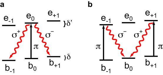
Figure 1: Model six-level atom, with $\pi$ transitions (straight lines) and $\sigma$ transitions (diagonal lines) displayed. The applied magnetic field creates ground- and excited-state frequency detunings, $\delta$ and $\delta^{\prime}$, respectively, between the $m=\pm 1$ and $m=0$ Zeeman sublevels.

Optical pumping prepares the atom in the state $|b_{0}\rangle$, after which, due to its interaction with the driven cavity mode, it is excited to the state $|e_{0}\rangle$. From here it may decay back to the ground state through the emission of a $\pi,\sigma^{+}$, or $\sigma^{-}$ photon. If the emission is of a $\pi$ photon, the emitted photon is added to the driven (V) mode; if, however, it is of a $\sigma^{+}+\sigma^{-}$ photon, it will populate the undriven (H) mode. In the latter case, assuming broadband detectors, when the photon is detected (measured in the H/V basis), the atom arrives in the superposition state

$$|\psi\rangle=(|b_{-1}\rangle+|b_{1}\rangle)/\sqrt{2}\,,$$ (1)

since neither the helicity nor the frequency of the photon is known. The coefficients of the superposition are the same because the probabilty of going from $|e_{0}\rangle$ to $|b_{-1}\rangle$ or $|b_{1}\rangle$ emitting an undriven photon is equal. This is because the ground- and excited-state Zeeman shifts are equal within the bandwidth of the cavity and cavity, drive and $\pi$ transition frequencies are assumed to be the same. Note that with the cavity decay rate comparable to the atom-cavity coupling, it is probable that the photon leaks from the cavity where it is detected before it can be reabsorbed. The atom now undergoes Larmor precession in the applied magnetic field while it continues to interact with the driven cavity mode. In this way the prepared ground state superposition appears in the excited state as the superposition

$$|\psi^{\prime}\rangle=(e^{-i\phi}|e_{-1}\rangle+e^{i\phi}|e_{1}\rangle)/\sqrt{2}\,$$ (2)

with the phase $\phi$ due to Larmor precession. From here the atom can return to its original state, $|b_{0}\rangle$, by emitting a second photon into the undriven (H) mode.

The conditional detection of both undriven-mode photons amounts to measuring the second-order correlation function, $g^{(2)}(\tau)$, of the H-polarized cavity output. Two indistinguishable paths yield “start” and “stop” photons for the measurement: $|b_{0}\rangle\rightarrow|e_{0}\rangle\rightarrow|b_{1}\rangle\rightarrow|e_{1}\rangle\rightarrow|b_{0}\rangle$ and $|b_{0}\rangle\rightarrow|e_{0}\rangle\rightarrow|b_{-1}\rangle\rightarrow|e_{-1}\rangle\rightarrow|b_{0}\rangle$. Since the phase advance along each path is different ($\pm\phi$), and the difference grows in time, interference between the paths yields oscillations, quantum beats, in $g^{(2)}(\tau)$. It is important to note that the quantum beats are not visible in the mean transmitted intensity of the undriven mode; a similar observation appears in Refs. [10, 11, 12] but for slightly different atomic or optical situations. They arise only when one conditions the “stop” photon detection on the preparation of the ground state superposition signaled by the “start” photon detection.

With our restriction to six atomic levels, the Hamiltonian for the atom interacting with the two orthogonally polarized cavity modes, written in a rotating frame, is

$$H=H_{0}+H_{I}+H_{cp}\,,$$ (3)

with

$$H_{0} = \hbar\delta^{\prime}(\sigma_{e_{-1}e_{-1}}-\sigma_{e_{1}e_{1}})+\hbar\delta(\sigma_{b_{-1}b_{-1}}-\sigma_{b_{1}b_{1}})\,,$$ (4)

$$H_{I} = -\hbar g\mkern-2.0mu\left[c_{0}\mkern 3.0mu\sigma_{e_{0}b_{0}}a_{1}+c_{0}^{\prime}\mkern 3.0mu(\sigma_{e_{1}b_{1}}+\sigma_{e_{-1}b_{-1}})a_{1}\right.$$ (5)

$$\left.c_{1}\mkern 3.0mu(\sigma_{e_{0}b_{1}}+\sigma_{e_{0}b_{-1}})a_{2}+c_{1}^{\prime}\mkern 3.0mu(\sigma_{e_{-1}b_{0}}+\sigma_{e_{1}b_{0}})a_{2}\right]+{\rm c.c.}\,,$$

$$H_{cp} = i\hbar\mathcal{E}(a_{1}^{\dagger}-a_{1})+i\hbar\xi_{b}(\hat{a}_{1}^{\dagger}a_{2}-\hat{a}_{2}^{\dagger}a_{1})\,,$$ (6)

where $\sigma_{ij}=|i\rangle\langle j|$ and $\mathcal{E}$ is the external drive of the V-polarized cavity mode. The term proportional to $\xi_{b}$ models cavity birefringence (in such a way that the coupled field amplitudes have the same phase). Operators $a_{1}$ and $a_{2}$ annihilate a photon in the driven and undriven modes, respectively, $g$ is the dipole coupling constant between the atom and the cavity field and the $c$s and $c^{\prime}$s are atom-field coupling coefficients.

Including now spontaneous emission and cavity decay, the master equation in the Lindblad form is

$$\dot{\rho}(t) = (1/i\hbar)[H,\rho]+\kappa L[a_{1}]+\kappa L[a_{2}]$$ (7)

$$+\frac{\gamma}{2}L[c_{0}\mkern 3.0mu\sigma_{b_{0}e_{0}}+c_{0}^{\prime}\mkern 3.0mu(\sigma_{b_{1}e_{1}}+\sigma_{b_{-1}e_{-1}})]$$

$$+\frac{\gamma}{2}L[\,c_{1}\mkern 3.0mu\sigma_{b_{0}e_{-1}}+c_{1}^{\prime}\mkern 3.0mu\sigma_{b_{1}e_{0}}\,]$$

$$+\frac{\gamma}{2}L[\,c_{1}^{\prime}\mkern 3.0mu\sigma_{b_{-1}e_{0}}+c_{1}\mkern 3.0mu\sigma_{b_{0}e_{1}}\,]\,,$$

with

$$L[o]=2o\rho o^{\dagger}-o^{\dagger}o\rho-\rho o^{\dagger}o\,,$$

where $\gamma$ is the spontaneous decay rate to modes other than the cavity modes and $\kappa$ is the cavity field decay rate.

We solve Eq. (7) using a truncated photon basis and use the so-called quantum regression theorem, in order to illustrate the main properties of the correlation function. We should note first that in equilibrium—i.e., considering the steady-state solution to Eq. (7)—the populations in states $|b_{0}\rangle$ and $|b_{i}\rangle$, $i=-1,1$, are all of the same order. In the limit of weak driving, and assuming the atom moves very slowly across the cavity, the system has three distinct, and widely different, time scales. The first, which governs the long-time evolution of the master equation to its steady state, is the time taken for the atomic ground states to reach equilibrium through optical pumping; this time goes to infinity as the drive strength, $\mathcal{E}$, approaches zero. The second is the time for the cavity field to reach a quasi-steady state, in equilibrium with the drive and the still slowly evolving atomic state. This shortest of the three time scales is of order $\kappa^{-1}$. The third, the intermediate time scale, is the time taken for the atom to transit the cavity. Our calculations assume that the first photon is detected after the transient on the shortest time scale has decayed—i.e., after the cavity field reaches its quasi-steady state. Then, while the atom transits the cavity, on the intermediate time scale, it is possible to guarantee that a first H-polarized photon detection leaves the atom in the superposition state of $|\psi\rangle$ of Eq. (1).

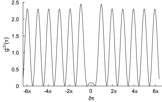
Figure 2: Normalized second-order correlation function of the undriven mode. The atom interacts with a fixed dipole coupling constant, $g$, for $\kappa/\gamma=1/2$, $g/\gamma=1/4$, $\delta/\gamma=1/2$, $\mathcal{E}/\gamma=1/64$, $c_{0}=\sqrt{4/7}$,$c_{0}^{\prime}=\sqrt{15/28}$,$c_{1}=-\sqrt{3/14}$,$c_{1}^{\prime}=-\sqrt{5/14}$.

Figure 2 displays an example of the computed second-order correlation function assuming a constant coupling between the atom and the cavity modes; the correlation function decays to unity on the (longest) optical pumping time scale. The quantum beats due to Larmor precession are prominently displayed, though they are suppressed around $\tau=0$ due to the antibunching of single-atom fluorescence (it is impossible for one atom to emit two photons within a single lifetime). Note that on applying the interaction Hamiltonian, Eq. (5), to the state $|\psi^{\prime}\rangle$, Eq. (2), the coupling between the atom and the undriven cavity mode vanishes for $\phi=(2n+1)\pi/2$, $n$ an integer; thus, an H-polarized photon cannot be emitted at these times, the origin of the interference zeros in Figure 2. For a Zeeman frequency shift $\delta$, the phase gained through Larmor precession in time $\tau$ is $\phi=\delta\tau$; hence the zeros occur for $\delta\tau=(2n+1)\pi/2$ with a frequency $2\delta$. In Fig. 2 the fringe visibility is maximal, as the probabilities for finding the atom in state $|b_{-1}\rangle$ or $|b_{1}\rangle$ are the same within our model. Engineering a different superposition, e.g., $|\psi\rangle=\alpha_{-1}|b_{-1}\rangle+\alpha_{1}|b_{1}\rangle$, with $|\alpha_{-1}|\neq|\alpha_{1}|$, would yield a lower visibility.

Our proposal differs from work done with similar schemes [13, 14, 15]. There are differences in the configuration: we use a CW laser to pump the cavity, which then drives the atom, and a magnetic field perpendicular to the cavity axis so that $\sigma^{+}$ and $\sigma^{-}$ photons cannot be distinguished. There are also qualitative differences. Rather than focusing on the generation of entangled photons and the transfer of information between the atom and light, we focus on atomic state manipulation. For this reason it is crucial to disentangle the atom from the field. The field is used to prepare and read the atomic state. We prepare the state with a measurement: the first photon detection prepares the system in the superposition, Eq. 1. This initialization disentangles the atom from the field and allows us, via feedback, to manipulate the atomic state alone. It shields the atomic state from alteration by a field measurement, making its manipulation less susceptible to errors. Instead of using quantum state tomography to infer the atomic state, we infer it from the phase and visibility of the second-photon fringe.

3 Manipulation of the quantum beats

3.1 Feedback protocol

Detection of the first photon prepares the superposition state which then evolves in the magnetic field. Quantum feedback similar to that of Refs. [6, 7] requires one to stop the Larmor oscillation of the atom in the ground state, and after a predetermined time continue it.

The quantum trajectory formalism [16] allows one to study the dynamics of a dissipative quantum system in real time. We show in this section what happens if, after a pre-set time, another laser beam excites one of the two parts of the superposition to a different state. The excitation interrupts the coherent evolution of the superposition. We envision it executed by a pulse of light which takes the specific ground-state magnetic sublevel to a different ground-state hyperfine (F) sublevel. The exciting pulse arrives from a direction perpendicular to the cavity axis and lasts for the appropriate time. The small detuning given by the magnetic field to the ground-state sublevels is large enough for selective excitation with a narrow laser or a two photon Raman transition. During the state transfer the external drive to the cavity is turned off.

There are two possible approaches to this excitation. One would be to excite to a state that cannot return in any way to the superposition. This simply interrupts the quantum beats so that the autocorrelation of the undriven mode reveals a sudden change in the dynamics—the oscillations cease; the interruption may be made at any time one chooses. A more interesting possibility is to use two Raman pulses to move the superposition in its entirety to another ground state while preserving the relative phase and with no spontaneous emission. A second pair of Raman pulses brings it back to resume the quantum beats. Figure 3 shows the computed correlation function, where the first arrow marks the time of the first state transfer and the second the time when the state is transferred back.

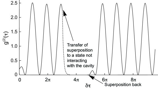
Figure 3: Manipulation of the quantum beats with quantum feedback. The first arrow indicates the time when the atomic state is transferred to a state that does not interact with the cavity modes. The dotted line indicates the decay of the now undriven cavity field. The second arrow indicates the time when the atomic state is brought back, and the quantum beats resume. Parameters as in the previous figure.

3.2 Probabilistic quantum error correction

The previous subsection illustrated the possibilities for quantum feedback on our system: one can interrupt the quantum beats and restart them later. We now go further and look at the possibility of applying the basic protocol to implement probabilistic error correction in Cavity QED. The idea developed derives from recent experiments with superconducting qubits [3, 4]. We first briefly describe how to correct an unwanted weak measurement using the probabilistic quantum error protocol described in Ref. [2] (see Ref. [5] for an optics application). Then we describe its implementation in our Cavity QED system.

Consider a qubit in the superposition $|\psi\rangle=\alpha_{0}|0\rangle+\alpha_{1}|1\rangle$, corresponding to the state of the atom after detecting a first undriven photon. If a weak measurement is performed to detect state $|1\rangle$ (weak in the sense that if the qubit is in $|1\rangle$, the probability $p$ to find the state is much less than unity), the effect of not detecting $|1\rangle$ is to partially collapse the superposition towards $|0\rangle$. In terms of the generalized measurement operators [17]

$$M_{a} = \sqrt{p}\mkern 3.0mu|1\rangle\langle 1|\,,$$ (8)

$$M_{b} = 1-\left(1-\sqrt{1-p}\mkern 3.0mu\right)|1\rangle\langle 1|\,,$$ (9)

the probability of detecting state $|1\rangle$ is $p_{1}=\langle\psi|M_{a}^{\dagger}M_{a}|\psi\rangle=p|\alpha_{1}|^{2}$, while the probability of not detecting it is $p_{0}=\langle\psi|M_{b}^{\dagger}M_{b}|\psi\rangle=1-p|\alpha_{1}|^{2}$. After the measurement, if we detect state $|1\rangle$, $|\psi\rangle$ collapses to $|1\rangle$. If we do not, we cannot deduce that the state of the system is $|0\rangle$; nevertheless, some information has been gained. This is easily seen from the fact that if we measure in a similar way an infinite number of times and never find the state $|1\rangle$, the deduction, then, most surely, is that the state is $|0\rangle$. Thus, after a first measurement, if we fail to find state $|1\rangle$, $|\psi\rangle$ is partially collapsed to

$$|\psi^{\prime}\rangle=\frac{M_{b}|\psi\rangle}{\sqrt{\langle\psi|M_{b}^{\dagger}M_{b}|\psi\rangle}}=\frac{\alpha_{0}|0\rangle+\alpha_{1}\sqrt{1-p}|1\rangle}{\sqrt{1-p|\alpha_{1}|^{2}}}\,.$$ (10)

The aim now is to correct the error introduced by the partial collapse. This may be done by performing the following operations: we swap $|0\rangle$ and $|1\rangle$ in $|\psi^{\prime}\rangle$ and repeat the measurement to detect state $|1\rangle$. The probability of a null result is now $(1-p)/(1-p|\alpha_{1}|^{2})$, and again, given the null result the state partially collapses to $|0\rangle$. Then swapping $|0\rangle$ and $|1\rangle$ for a second time the original state, $|\psi\rangle$, is recovered. The probability of recovery after the two measurements is $(1-p)$.

What if we do not know the outcome of the measurements? In this case the density operator formalism can account for our ignorance. The total Hilbert space is $H_{q}\otimes H_{d}$, where $H_{q}$ is the two dimensional Hilbert space of the qubit and $H_{d}$ is the detector Hilbert space. The initial detector state is $|{\rm no}\rangle$, and if it detects the state $|1\rangle$ it changes to $|{\rm yes}\rangle$. The initial state of the qubit plus detector is $|\psi\rangle|{\rm no}\rangle$. After the first measurement the state of the system is

$$\rho=(1-p|\alpha_{1}|^{2})\left(|\psi^{\prime}\rangle\langle\psi^{\prime}|\right)\left(|{\rm no}\rangle\langle{\rm no}|\right)+p|\alpha_{1}|^{2}\left(|1\rangle\langle 1|\right)\left(|{\rm yes}\rangle\langle{\rm yes}|\right)\,,$$ (11)

and after the second measurement,

$$\rho^{\prime}=(1-p)\left(|\psi\rangle\langle\psi|\right)\left(|{\rm no}\rangle\langle{\rm no}|\right)+p\left(|1\rangle\langle 1|\right)\left(|{\rm yes}\rangle\langle{\rm yes}|\right)\,.$$ (12)

In this case the swapping of $|0\rangle$ and $|1\rangle$ must be carried out independently of the measurement outcomes which are assumed unknown. Still, there is a probability $1-p$ that the detector recorded two negative answers and the system is in state $|\psi\rangle|{\rm no}\rangle$ and a probability $p$ that it recorded a positive answer (at least one) and the system is in state $|1\rangle|{\rm yes}\rangle$.

3.3 Implementation in cavity QED

In order to implement the protocol in cavity QED we define $|b_{1}\rangle$ and $|b_{-1}\rangle$ as the states of the qubit. The measurement of a first undriven mode photon then starts a series of pulses (e.g., inducing Raman transitions between the qubit states) that initializes the state

$$|\psi\rangle=\alpha_{0}|b_{-1}\rangle+\alpha_{1}|b_{1}\rangle\,.$$ (13)

In order to verify the preparation, the qubit state information may be mapped in $H$-polarized photons, with the state of the qubit obtained from the visibility and phase of the autocorrelation function. Using the predictability $\mathcal{P}={\rm mod}(|\langle b_{-1}|\psi\rangle|^{2}-|\langle b_{1}|\psi\rangle|^{2})$ and the visibility $\mathcal{V}$, we have numerically checked for the parameters used in this paper that

$$\mathcal{P}^{2}+\mathcal{V}^{2}\approx 1\,.$$ (14)

This is an analog of the inequality characterizing a two-way interferometer [18], and it allows us to determine the relative probability to occupy the qubit states from the fringe visibility. The relative phase of the state amplitudes is carried by the phase of the quantum beats. The weak measurement might be implemented by a pulse of light, such that if the atom is in state $|b_{1}\rangle$ there is a probability $p\ll 1$ of it being ionized. If the atom is ionized (probability $p|\alpha_{1}|^{2}$), the unitary inverse operation is impossible, i.e., the pulse makes a measurement with outcome “yes”. If we do not know the outcome, the system density operator is

$$\rho=(1-p|\alpha_{1}|^{2})\left(|\psi^{\prime}\rangle\langle\psi^{\prime}|\right)\left(|{\rm no}\rangle\langle{\rm no}|\right)+p|\alpha_{1}|^{2}\left(|{\rm ion}\rangle\langle{\rm ion}|\right)\left(|{\rm yes}\rangle\langle{\rm yes}|\right)\,,$$ (15)

where $|{\rm ion}\rangle$ is the state of the ionized atom. If the atom is ionized, the cavity no longer interacts with the atom and no second photon is emitted. Otherwise, a second photon may be emitted, with the resulting quantum beats having a visibility determined by the state $|\psi^{\prime}\rangle$.

The state $|\psi\rangle$ is recovered in the manner outlined above: after the first weak measurement, we swap states $|b_{1}\rangle$ and $|b_{-1}\rangle$, and then repeat the weak measurement and swap the states again. The final density operator is

$$\rho^{\prime}=(1-p)\left(|\psi\rangle\langle\psi|\right)\left(|{\rm no}\rangle\langle{\rm no}|\right)+p\left(|{\rm ion}\rangle\langle{\rm ion}|\right)\left(|{\rm yes}\rangle\langle{\rm yes}|\right)\,.$$ (16)

Note that with a probability $1-p$ the atom was not ionized and the state of the system is $|\psi\rangle$. If a second photon is detected, the $g^{(2)}(\tau)$ constructed from these events will correspond to the original state $|\psi\rangle$. The visibility will be as if no weak measurements were performed. The modification of the state introduced by the first measurement is corrected by the second. The probability for the scheme to be successful is $1-p$. The visibility diminishes in the case where $|\psi\rangle$ has equal coefficients if the protocol is not implemented after the first weak measurement. The recovery of the initial maximal visibility is a necessary signature that the protocol is working.

The experimental realization of the probabilistic quantum error correction protocol in superconducting phase qubits [4] requires knowing the probability of success of the partial measurement in order to correctly estimate the recovered quantum state. In the presented scheme this is not needed.

4 Experimental proposal and sensitivity analysis for atoms from an atomic beam

This section briefly describes the experimental apparatus where this proposal can be implemented, and analyzes the sensitivity of the measured correlation function to certain experimental realities. Since the correlation function carries all the information required for the proposed quantum feedback and error correction, it is important to compute it for the realistic situation where atoms are provided by an atomic beam. Such atoms are produced with random arrival times, velocities, and directions of motion through the cavity mode function. We also comment on a number of other experimental considerations that might diminish the visibility of the quantum beats, or alter their frequency.

Our experimental apparatus consists of a $2\mkern 2.0mu{\rm mm}$ Fabry-Perot cavity and a source of cold ⁸⁵Rb atoms [19, 20]. The source delivers, on average, less than the equivalent of one maximally coupled atom within the mode volume of the cavity at all times. The cavity supports two degenerate modes of orthogonal linear polarization (H and V). During their transit, the atoms interact with the orthogonally polarized modes for approximately $5\mkern 2.0mu\mu{\rm s}$. (See Refs. [21, 22] for similar systems.) In the presence of a weak magnetic field, and with the appropriate choice of hyperfine levels, the atomic structure of Rb allows for the separation of spontaneous emission events in the cavity. Driving $\pi$ transitions with V polarization means that any light emitted along the cavity axis with H polarization must come from spontaneous decay via a linear superposition of $\sigma^{+}$ and $\sigma^{-}$ light.

We use in the atom-field interaction the Clebsch-Gordon coefficients coupling the central six sublevels of the $D_{2}$ line of ⁸⁵Rb on the $F=3$ to $F=4$ transition, i.e., we impose a truncation of the full atomic raising and lowering operators. The justification for this truncation is as follows. Atoms interact with the cavity field for a finite time in the experiment. Their coupling to the field changes as a function of position as they transit the cavity. This limits the time over which a given atom can emit two photons, imposing a limit on the duration of the observed quantum beats. Due to the weak pump field, the period of a Rabi oscillation between the ground and excited levels is much larger than the time the atom interacts with the cavity. The spreading of the population to states outside the considered manifold, before and after the first photon measurement, is negligible; moreover, the proposed manipulations of the atomic state remains inside the considered manifold.

In the weak limit at most two undriven photons are emitted by each atom inside the cavity. When the second photon is emitted from $\psi^{\prime}$, Eq. (2), the atom can finish in a state different to $b_{0}$, thus reducing the fringe visibility. An estimation of how much the visibility decreases can be obtained from the Clebsch-Gordon coefficient that couples states $e_{\pm 1}$ with states $b_{\pm 2}$. The transition probability from $\psi^{\prime}$ to any of the ground states yields a visibility of $5/8$ instead of $1$. The fact that the fringe does not disappear altogether can be understood in the following way. When the phase of $\psi^{\prime}$ is $\phi=n\pi$, $n$ an integer—i.e. when the probability for a second photon emission is maximum—the photon leaves the truncated six-fold manifold with probability $3/13$; nevertheless, in the majority of the cases (probability $10/13$) it contributes to the quantum beats.

We model the source of atoms as a dilute atomic beam, assuming that the cavity is either empty of atoms or occupied by one atom at the most. The atomic trajectories and interaction volume are defined in an manner similar to that of Ref. [23]. The mean intracavity photon number of the undriven mode in steady state is

$$\overline{\langle a_{2}^{\dagger}a_{2}\rangle}=\overline{(\overline{N}/t_{j})\int_{0}^{t_{j}}\langle a_{2}^{\dagger}a_{2}(t)\rangle dt}\,,$$ (17)

where $\overline{N}$ is the mean number of atoms in the interacting volume (probability to find an atom in the cavity) and the integral performs a time average over the passage of atom $j$ through the cavity mode function, with transit time $t_{j}$ and time-dependent coupling $g_{j}(t)$. The overbar denotes the average over an ensemble of atoms $\{j\}$. Similarly, we calculate the unnormalized correlation function in steady state as

$$\overline{G^{(2)}(\tau)}=\overline{(\overline{N}/t_{j})\int_{0}^{t_{j}}\langle a_{2}^{\dagger}(t)a_{2}^{\dagger}(t+\tau)a_{2}(t+\tau)a_{2}(t)\rangle dt}\,.$$ (18)

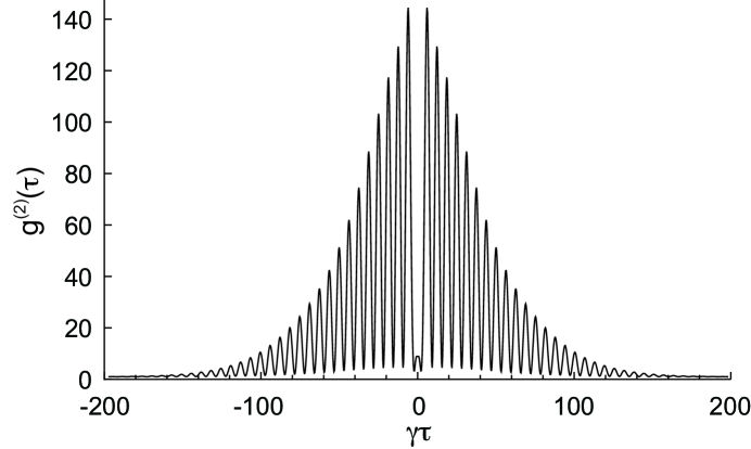
Figure 4: Montecarlo simulation of the undriven normalized second-order correlation function for a cavity with waist $w=56\mu$m and linewidth $\lambda=780$ nm. The Low-Velocity source of atoms has mean velocity $\overline{v}=15$ m/s with deviation $\Delta v=1.1$ m/s. The parallel and transverse (to the cavity axis) divergence angles are $\Delta\theta_{p}=1/40$ and $\Delta\theta_{t}=1/80$ respectively. Other parameters: $\gamma/2\pi=6$ MHz, $\kappa/\gamma=1/2$, $g/\gamma=1/4$, $\delta/\gamma=1/2$, $\overline{N}=0.1$, $\mathcal{E}/\gamma=1/16$, $c_{0}=\sqrt{4/7}$, $c_{0}^{\prime}=\sqrt{15/28}$, $c_{1}=-\sqrt{3/14}$, $c_{1}^{\prime}=-\sqrt{5/14}$.

The transit time imposes a limit on the duration of the observed quantum beats compared with the ongoing beats of Fig. 2. So long as the external drive is weak, the atom transit time is the only source of “decoherence” in the system; the finite lifetime of the atomic excited state and of photons in the cavity does not limit the duration of the quantum beats, nor does any optical pumping under the weak drive limit.

For each trajectory, the atom-cavity coupling—hence $G^{(2)}(\tau)$—goes to zero as $\tau$ goes to infinity. In reality atoms enter and leave the cavity continuously, so different atoms provide “start” and “stop” photons at long delays and the correlation function does not go to zero. Assuming at most one atom in the cavity at a time, and a mean time between atoms much larger than the photon lifetime in the cavity, the normalized autocorrelation function can be written as

$$g^{(2)}(\tau)=1+\overline{G^{(2)}(\tau)}/\left(\overline{\langle a_{2}^{\dagger}a_{2}\rangle}\mkern 3.0mu\right)^{2}\,,$$ (19)

where the background of unity comes from the correlation of photons emitted by different atoms, while the term rising above unity correlates photons from the same atom. Since the restriction to one atom at a time requires $\overline{N}\ll 1$, the so-normalized quantum beat has an amplitude much greater than unity.

Equation 19 calculates the second-order correlation function under the assumption of only one atom in the cavity at any time; it draws upon the one-atom $g^{(2)}(\tau)$ only. There are other cases where an $N$-atom correlation function can be written as a sum of one-atom correlation functions. Specifically, when $N$ independent atoms emit simultaneously, the second-order correlation function of their total emitted field is a sum of terms involving the one-atom $g^{(1)}(\tau)$ as well as the $g^{(2)}(\tau)$ [24, 25]. Since we assume there is never more than one atom in the cavity, and the atoms are separated by $t\gg 1/\kappa$, terms involving $g^{(1)}(\tau)$ do not appear in Eq. 19. We note that Eq. (11) of Ref.[24] yields our result when $\bar{N}\ll 1$.

Figure 4 shows an example of the autocorrelation function obtained from Eq. 19. The beam geometry (1.5 mm hole in the MOT, 4.5 cm distance to the cavity and 2 mm mirror spacing) give parallel and transverse (to the cavity axis) divergence angles of $\Delta\theta_{p}\approx 1/40$ and $\Delta\theta_{t}\approx 1/80$ respectively. The distribution of speeds is assumed to be Gaussian with mean $\overline{v}=15$m/s and width $\Delta v=1.1$m/s. The angle distribution is assumed to be triangular, as is the case for a low-velocity source of atoms from magneto-optical traps (MOT) [26].

If the variation of the cavity-atom coupling is small between adjacent maxima and minima (i.e., $1/t_{j}\ll 2\delta$), then Eq. (14) still holds. For each atomic trajectory, under weak drive and with only one atom in the cavity at a time, one may calculate the visibility over the first two oscillations of $g^{(2)}(\tau)$ before the transit time affects the visibility significantly. Under these conditions, the quantum beats are in phase, regardless of the path and speed of the atom. Averaging trajectories with the same visibility does not change the final result.

The visibility of the quantum beats is maximal and constant for a weak drive. Increasing the drive strength brings a decrease in the visibility and an increased decay rate of the oscillations. Given a photon detection at $\tau=0$, the probability for detecting the very next photon still exhibits quantum beats; however, uncorrelated photons contribute at longer delays. These, for example, might come from the repeated absorption and emission of $V$- and $H$-polarized photons, respectively; such events reinitialize the quantum beat with altered phase; higher drive strength increases their number and decreases the visibility. Also, spontaneous emission into modes other than those of the cavity may cause decay from $|e_{0}\rangle$ to the ground state without providing a heralding photon in the undriven cavity mode. Following such an emission, the atom might be reexcited and returned to $|b_{0}\rangle$, now emitting a photon into the undriven cavity mode. This photon, not being preceded by a correlated “start”, further diminishes the visibility. When the driving is sufficiently weak, the number of uncorrelated detections approaches zero and maximum visibility is obtained.

To ensure that the decay of the quantum beats is due to the transit of the atom across the cavity rather than a strong drive, our model shows, for the parameters used, that the number of photons inside the cavity must be less than approximately four times the saturation photon number.

We have also verified that so long as any detuning between the $\pi$ atomic transition (or the drive) and the cavity frequency is smaller than the cavity width, the frequency of the quantum beats is unaltered. Furthermore, for a weak drive, unequal Zeeman shifts in the ground and excited states ($\delta\neq\delta^{\prime}$) do not significantly alter the quantum beat frequency; it reflects the Larmor frequency of the ground state.

Of more concern from an experimental point of view is the possible presence of birefringence in the cavity. This works as a direct coupling between its two orthogonally polarized modes. We model it by introducing such a coupling term in the system Hamiltonian [Eq. (3)]. The most important differences that this modeling shows are the disappearance of the antibunching around $\tau=0$ and a change of the quantum beat frequency from twice the Larmor frequency to the Larmor frequency itself. The frequency change occurs when the field generated by birefringence is approximately half the undriven field generated by the atom.

A final important issue is the effect of two or more atoms in the cavity at a time. A thorough treatment is reserved for future work. We have, however, obtained some preliminary indications. Restricting the atomic basis to $N$- atom symmetric states, we find, in the limit of weak driving and for the parameters used throughout this paper, that neither the frequency nor duration of the quantum beats depends on $N$. This follows because the underlying beat mechanism is independent of $N$.

5 Conclusions

We have shown in this paper that a cavity QED system comprising two orthogonally polarized modes coupled to an atom with magnetic structure shows robust quantum beats at twice the Larmor frequency of the atomic ground state. The beats are only visible through conditional measurement of the intensity of the undriven mode, i.e., as photon correlations. They allow for control and feedback of ground state superpositions created on the detection of a spontaneously emitted “start” photon. Realistic experiments have been proposed which can be implemented in current realizations of cavity QED in the optical regime. They open a path to new quantum error correction protocols and also a new class of quantum feedback and control.

Work supported by CONACYT, México, NSF of the United States, and the Marsden Fund of RSNZ of New Zealand.

6 References

References

- [1] H M Wiseman and G J Milburn. Quantum Measurement and Control. Cambridge University Press, Cambridge, 2009.
- [2] M Koashi and M Ueda. Reversing measurement and probabilistic quantum error correction. Phys. Rev. Lett., 82:2598, 1999.
- [3] A N Korotkov and A N Jordan. Undoing a weak quantum measurement of a solid-state qubit. Phys. Rev. Lett., 97:166805, 2006.
- [4] N Katz, M Neeley, M Ansmann, M Hofheinz R C Bialczak, E Lucero, A O’Connell, H Wang, A N Cleland, J M Martinis, and A N Korotkov. Reversal of the weak measurement of a quantum state in a superconducting phase qubit. Phys. Rev. Lett., 101:200401, 2008.
- [5] Y-S Kim, Y-W Cho, Y-S Ra, and Y-H Kim. Reversing the weak quantum measurement for a photonic qubit. Opt. Exp., 17(14):11978 – 11985, 2009.
- [6] W P Smith, J E Reiner, L A Orozco, S Kuhr, and H M Wiseman. Capture and release of a conditional state of a cavity QED system by quantum feedback. Phys. Rev. Lett., 89:133601, 2002.
- [7] J E Reiner, W P Smith, L A Orozco, H M Wiseman, and J Gambetta. Quantum feedback in a weakly driven cavity qed system. Phys. Rev. A, 70:0238119, 2004.
- [8] J I Cirac, P Zoller, H J Kimble, and H. Mabuchi. Quantum state transfer and entanglement distribution among distant nodes in a quantum network. Phys. Rev. Lett., 78:3221, 1997.
- [9] M O Scully and K Drühl. Quantum eraser: A proposed photon correlation experiment concerning observation and ‘delayed choice’ in quantum mechanics. Phys. Rev. A, 25:2208, 1982.
- [10] J Javanainen. Effect of state superpositions created by spontaneous emission on laser-driven transitions. Europhys. Lett., 17(5):407–412, 1992.
- [11] G C Hegerfeldt and M B Plenio. Coherence with incoherent light: A new type of quantum beat for a single atom. Phys. Rev. A, 47(3):2186–2190, Mar 1993.
- [12] A K Patnaik and G S Agarwal. Cavity-induced coherence effects in spontaneous emissions from preselection of polarization. Phys. Rev. A, 59:3015 – 3020, 1999.
- [13] T Wilk, S C Webster, H P Specht, G Rempe, and A Kuh. Polarization-controlled single photons. Phys. Rev. Lett., 98:063601, 2007.
- [14] T Wilk, S C Webster, A Kuhn, and G Rempe. Single-atom single-photon quantum interface. Science, 317:488, 2007.
- [15] B Weber, H P Specht, T Müller, J Bochmann, M Mücke, D L Moehring, and G Rempe. Photon-photon entanglement with a single trapped atom. Physical Review Letters, 102(3):030501, 2009.
- [16] H J Carmichael. An Open Systems Approach to Quantum Optics, Lecture Notes in Physics, volume 18. Springer-Verlag, Berlin, 1993.
- [17] M A Nielsen and I L Chuang. Quantum Computation and Quantum Information. Cambridge University Press, Cambridge, 2000.
- [18] B G Englert. Fringe visibility and which-way information: An inequality. Phys. Rev. Lett., 77(11):2154–2157, Sep 1996.
- [19] M L Terraciano, R Olson Knell, D L Freimund, L A Orozco, J P Clemens, and P R Rice. Enhanced spontaneous emission into the mode of a cavity qed system. Opt. Lett., 32:982, 2007.
- [20] M L Terraciano, R Olson Knell, D G Norris, J Jing, A Fernández, and L A Orozco. Photon burst detection of single atoms in an optical cavity. Nat. Phys., 5:480–484, 2009.
- [21] K M Birnbaum, A Boca, R Miller, A D Boozer, T E Northup, and H J Kimble. Photon blockade in an optical cavity with one trapped atom. Nature, 436:87, 2005.
- [22] T Aoki, A S Parkins, D J Alton, C A Regal, B Dayan, E Ostby, K J Vahala, and H J Kimble. Efficient routing of single photons by one atom and a microtoroidal cavity. Phys. Rev. Lett., 102:083601, 2009.
- [23] L Horvath and H J Carmichael. Effect of atomic beam alignment on photon correlation measurements in cavity QED. Phys. Rev. A, 76:043821, 2007.
- [24] H J Carmichael, P Drummond, P Meystre, and D F Walls. Intensity correlations in resonance fluorescence with atomic number fluctuations. J. Phys. A: Math. Gen., 11:L121–L126, 1978.
- [25] M Hennrich, A Kuhn, and G Rempe. Transiton from antibunching to bunching in cavity qed. Phys. Rev. Lett., 94:053604, 2005.
- [26] Z T Lu, K L Corwin, M J Renn, M H Anderson, E A Cornell, and C E Wieman. Low-velocity intense source of atoms from a magneto-optical trap. Phys. Rev. Lett., 77:3331, 1996.