Discrete diffraction and shape-invariant beams in optical waveguide arrays

Abstract

General properties of linear propagation of discretized light in homogeneous and curved waveguide arrays are comprehensively investigated and compared to those of paraxial diffraction in continuous media. In particular, general laws describing beam spreading, beam decay and discrete far-field patterns in homogeneous arrays are derived using the method of moments and the steepest descend method. In curved arrays, the method of moments is extended to describe evolution of global beam parameters. A family of beams which propagate in curved arrays maintaining their functional shape -referred to as discrete Bessel beams- is also introduced. Propagation of discrete Bessel beams in waveguide arrays is simply described by the evolution of a complex $q$ parameter similar to the complex $q$ parameter used for Gaussian beams in continuous lensguide media. A few applications of the $q$ parameter formalism are discussed, including beam collimation and polygonal optical Bloch oscillations.

I Introduction

Linear and nonlinear propagation of ’discretized’ light in arrays of evanescently-coupled optical waveguides has received a great and increasing interest in the past recent years (see, for instance, Christodoulides03 ; Lederer08 and references therein). As compared to diffraction or refraction in continuous (non-structured) media, discrete diffraction and refraction in waveguide arrays show rather uncommon effects which result from the evanescent coupling among adjacent waveguides forming a one-dimensional or a two-dimensional lattice. For instance, linear propagation of light waves in homogeneous arrays may show diffraction reversal and self-collimation effects Eisenberg00 ; Pertsch02 , anomalous refraction Pertsch02 , the discrete Talbot effect Iwanow05 , and quasi-incoherent propagation SzameitAPL07 to name a few. Remarkably, discrete diffraction can be tailored by properly introducing inhomogeneities in the lattice or by varying its topology. In particular, since the first proposals and demonstrations of optical Bloch oscillations Peschel98 ; Morandotti99 ; Lenz99 and ’diffraction management’ in zig-zag arrays Eisenberg00 , the use of waveguide arrays with curved optical axis has been extensively investigated both theoretically and experimentally, with the demonstration of diffraction suppression via Bloch oscillations Christodoulides03 ; Peschel98 ; Morandotti99 ; Lenz99 ; Usievich04 or dynamic localization Lenz03 ; Longhi05 , polychromatic diffraction management Garanovich06 , astigmatic diffraction control Garanovich07 , multicolor Talbot effect Garanovich06 , and discrete soliton management Musslimani01 . Linear and nonlinear light propagation at the surface or at the interface of two waveguide lattices also exhibits a variety of interesting properties which have been investigated in several recent works (see, for instance, Lederer08 ; surf1 ; surf2 ; surf3 and references therein). In spite of such a great amount of works, some facets of discrete diffraction, even in the simplest linear propagation regime, have been overlooked. Though in the linear regime the impulse response (Green function) of the array may be rather generally calculated analytically -either in straight or curved geometries and in presence or not of boundaries- and its knowledge is enough to predict light evolution for any assigned initial excitation condition (see, for instance, Longhi05 ; surf1 ), some general issues of discrete diffraction, which are well known for paraxial propagation of beams in continuous media, have not been comprehensively addressed, including: (i) a description of global beam parameter evolution in a closed analytical form; (ii) far-field discrete diffraction in homogeneous array (the analogue of Fraunhofer diffraction in homogeneous continuous media); (iii) the general scaling law of beam broadening and beam decay, especially close to the self-collimation condition (also referred to as sub-diffraction) which is commonplace to the more general class of photonic crystal structures (see, for instance, Kosaka99 ); (iv) the existence of shape-invariant discretized beams, i.e. special families of field distributions which -like Gaussian beams in continuous lensguide media- do propagate in straight or curved waveguide arrays maintaining their functional shape. It is the aim of this work to shed some light into such issues. In particular, it is shown rather generally that: (i) the scaling law describing broadening of discretized light in homogeneous arrays is the same as that of standard paraxial diffraction theory of homogeneous continuous media (beam size asymptotically grows linearly with propagation distance), independently of the precise array dispersion curve and even along self-collimation directions; (ii) in a homogenous array, the discrete far-field pattern is not the (discrete) Fourier transform of the near-field distribution, and the scaling law of beam decay may depend on the observation angle; (iii) special field distributions, which propagate in straight or curved waveguide arrays maintaining their functional shape and referred to as ’discrete Bessel beams’, can be introduced for simple tight-binding waveguide models; (iv) a discrete Bessel beam is defined by a complex $q$ parameter, analogous to the one used for Gaussian beams in continuous lensguide media, and propagation of the $q$ parameter along the array admits of a simple geometric interpretation.
The paper is organized as follows. In Sec.II general properties of discrete diffraction in homogeneous waveguide arrays are presented, including the derivation of the general scaling laws of beam broadening and beam decay, far-field discrete diffraction, with a a note on self-collimation regimes. In Sec.III, some general rules of beam propagation in curved waveguide arrays are derived within the nearest-neighbor coupling approximation, whereas in Sec.IV the family of shape-invariant discrete Bessel beams is introduced, together with the complex $q$ parameter formalism. Applications to beam collimation and polygonal optical Bloch oscillations are also presented. Finally, in Sec.V the main conclusions are outlined.

II Discrete diffraction in a homogeneous waveguide array

II.1 Continuous model of discrete diffraction

The starting point of our analysis is provided by a rather standard model describing linear propagation of monochromatic light waves along the $z$ direction of a one-dimensional or two-dimensional array of waveguides in the single band and tight-binding approximations. For instance, in a one-dimensional array such conditions are satisfied when the tilt of beams and waveguides at the input facet is less than the Bragg angle, so that the lowest-order band of the array is excited and beam propagation is primarily characterized by coupling between the fundamental modes of the waveguides. For a two-dimensional array, the relevant equations describing discrete diffraction in a single band approximation read

$$i\dot{c}_{n,m}=-\sum_{l,r}\Delta_{n-l,m-r}c_{l,r}$$ (1)

where $c_{n,m}(z)$ is the complex amplitude of the fundamental waveguide mode at the lattice site $\mathbf{r}_{n,m}=n\mathbf{a}+m\mathbf{b}$ identified by the indices $(n,m)$, $\mathbf{a}$ and $\mathbf{b}$ are the lattice vectors of the unit cell, the dot denotes the derivative with respect to $z$, and $\Delta_{n,m}=\Delta_{m,n}^{*}$ are the coupling rates. In order to derive a general rule of beam broadening due to discrete diffraction, it is worth introducing a continuous field envelope $\psi(x,y,z)$ satisfying the scalar Schrödinger-like equation

$$i\partial_{z}\psi(\mathbf{r},z)=H_{0}(\mathbf{p})\psi\mathbf{(r},z),$$ (2)

where $\mathbf{r}=(x,y)$, $\mathbf{p}=-i\nabla_{\mathbf{r}}$,

$$H_{0}(\mathbf{p})\equiv-\sum_{n,m}\Delta_{n,m}\exp\left(-i\mathbf{r}_{n,m}\cdot\mathbf{p}\right),$$ (3)

and $\mathbf{r}_{n,m}=n\mathbf{a}+m\mathbf{b}$. Taking into account that $\exp(-i\mathbf{R}\cdot\mathbf{p})\psi(\mathbf{r},z)=\psi(\mathbf{r+R},z)$, it follows that the solution $c_{n,m}(z)$ to the discrete equation (1) can be identified with $\psi(\mathbf{r}=n\mathbf{a}+m\mathbf{b},z)$. The formulation of the discrete light propagation problem [Eq.(1)] as a continuous problem [Eq.(3)] is a well-established procedure in solid-state physics Ziman which enable the use of certain analytical techniques, such as the method of moments, developed for the continuous Schrödinger equation or for the paraxial wave equation (see, for instance, Krivoshlykov ; Styer90 ). In addition, the continuous model includes, as a particular case, the problem of paraxial diffraction in a homogeneous medium (e.g. in the vacuum), which is attained by simply assuming for the Hamiltonian $H_{0}(\mathbf{p})$, in place of Eq.(3), the (normalized) parabolic form

$$H_{0}(\mathbf{p})=\frac{\mathbf{p}^{2}}{2}.$$ (4)

The normalization conditions $\int d\mathbf{r}|\mathbf{\psi}\mathbf{(r},z)|^{2}=1$ for Eq.(2), and $\sum_{n,m}|c_{n,m}(z)|^{2}=1$ for the discrete problem (1), will be assumed in the following analysis.

II.2 General law for beam spreading: moment analysis

Two global parameters describing beam propagation are the beam center of mass $\langle\mathbf{r}\rangle=\langle x\rangle\mathbf{u}_{x}+\langle y\rangle\mathbf{u}_{y}$ and the transverse beam spot sizes $w_{x}(z)$ and $w_{y}(z)$ defined by

$$\langle\mathbf{r}\rangle=\int d\mathbf{r}\mathbf{r}|\psi(\mathbf{r},z)|^{2},$$ (5)

$$w_{x}(z) = \sqrt{\langle x^{2}\rangle-\langle x\rangle^{2}}$$ (6)

$$w_{y}(z) = \sqrt{\langle y^{2}\rangle-\langle y\rangle^{2}}$$ (7)

where

$$\langle x^{2}\rangle(z)=\int d\mathbf{r}x^{2}|\psi(\mathbf{r},z)|^{2}\;,\;\langle y^{2}\rangle(z)=\int d\mathbf{r}y^{2}|\psi(\mathbf{r},z)|^{2}.$$ (8)

Note that the above definitions hold for both continuous and discrete diffraction models. In the latter case, assuming $\psi(\mathbf{r},z)$ to be a piecewise constant function in each cell of the lattice and taking $|\mathbf{a}\times\mathbf{b}|=1$ for the area of the unit cell, the integral over $\mathbf{r}$ may be replaced by a double sum over the cell indices $n$ and $m$, i.e. in the discrete model one has $\int d\mathbf{r}\rightarrow\sum_{m,n}$.
The evolution equations for $\mathbf{r}$ and $w_{x,y}$ can be readily obtained in a closed form by writing a set of Eherenfest equations for the expectation values of $\mathbf{\mathbf{r}}$, $x^{2}$, $y^{2}$, and of commutator operators that arise in the calculation. The expectation value $\langle A\rangle\equiv\int d\mathbf{r}\psi^{*}(\mathbf{r},z)A(\mathbf{r},\mathbf{p})\psi(\mathbf{r},z)$ of any operator $A(\mathbf{r},\mathbf{p})$ (not necessarily self-adjoint) evolves according to

$$\frac{d\langle A\rangle}{dz}=-i\langle[A,H_{0}]\rangle$$ (9)

and the following commutation relations

$$[\mathbf{r},f(\mathbf{p})]=i\nabla_{\mathbf{p}}f\;,\;[g(\mathbf{r}),\mathbf{p}]=i\nabla_{\mathbf{r}}g$$ (10)

hold for any functions $f(\mathbf{p})$ and $g(\mathbf{r})$. For $A=\mathbf{r}$, one obtains

$$\frac{d\langle\mathbf{r}\rangle}{dz}=\langle\nabla_{\mathbf{p}}H_{0}\rangle,\;\frac{d\langle\nabla_{\mathbf{p}}H_{0}\rangle}{dz}=0,$$ (11)

i.e.

$$\langle\mathbf{r}\rangle(z)=\langle\mathbf{r}\rangle(0)+\langle\nabla_{\mathbf{p}}H_{0}\rangle z$$ (12)

which is the evolution equation of the beam center of mass. Note that the path followed by any beam is always straight, regardless of the specific form of $H_{0}$ or initial field distribution which just determine the transverse drift velocity $\langle\nabla_{\mathbf{p}}H_{0}\rangle$ of the beam. To determine the evolution equation of the beam spot size $w_{x}$, let us assume $A=x^{2}$, so that the following cascade of Eherenfest equations [Eq.(9)] is obtained

$$\frac{d\langle x^{2}\rangle}{dz} = \langle x\frac{\partial H_{0}}{\partial p_{x}}+\frac{\partial H_{0}}{\partial p_{x}}x\rangle$$ (13)

$$\frac{d}{dz}\langle x\frac{\partial H_{0}}{\partial p_{x}}+\frac{\partial H_{0}}{\partial p_{x}}x\rangle = 2\langle\left(\frac{\partial H_{0}}{\partial p_{x}}\right)^{2}\rangle$$ (14)

$$\frac{d}{dz}\langle\left(\frac{\partial H_{0}}{\partial p_{x}}\right)^{2}\rangle = 0.$$ (15)

After integration, one obtains

$$\langle x^{2}\rangle(z)=\langle x^{2}\rangle(0)+\langle x\frac{\partial H_{0}}{\partial p_{x}}+\frac{\partial H_{0}}{\partial p_{x}}x\rangle z+\langle\left(\frac{\partial H_{0}}{\partial p_{x}}\right)^{2}\rangle z^{2},$$ (16)

where the expectation values on the right hand side of Eq.(16) are calculated at $z=0$, i.e. for the initial beam distribution. From Eqs.(6), (12) and (16) the following evolution equation for the beam spot size $w_{x}$ is then obtained

$$w_{x}^{2}(z)=w_{x}^{2}(0)+\alpha_{x}z+\beta_{x}^{2}z^{2},$$ (17)

where we have set

$$\alpha_{x}=\langle(x-\langle x\rangle)\frac{\partial H_{0}}{\partial p_{x}}+\frac{\partial H_{0}}{\partial p_{x}}(x-\langle x\rangle)\rangle,$$ (18)

$$\beta_{x}^{2}=\langle\left(\frac{\partial H_{0}}{\partial p_{x}}\right)^{2}\rangle-\left(\langle\frac{\partial H_{0}}{\partial p_{x}}\rangle\right)^{2}$$ (19)

and the expectation values are calculated at $z=0$. A similar expression for $w_{y}(z)$ can be obtained by replacing $x$ with $y$ in Eqs.(17), (18) and (19). A major result expressed by Eq.(17) is that, regardless of the particular form of $H_{0}$, $w_{x}(z)$ (and similarly $w_{y}(z)$) asymptotically grows with $z$ linearly, with a diffraction length given by $\sim 1/\beta_{x}$. Therefore -and this one of the major result of this section- the broadening law of a spatial beam due to diffraction does not differ for discrete or continuous diffraction. In addition, for a beam carrying a finite power and admitting of finite moments $\langle x^{2}\rangle$ and $\langle y^{2}\rangle$, the coefficient $\beta_{x}^{2}$ given by Eq.(19) is always strictly positive and does not vanish. This can be generally proven by observing that $\beta_{x}^{2}$ is the variance of the operator $(\partial H_{0}/\partial p_{x})$, which is always positive and vanishes solely when the initial field distribution $\psi(x,y,0)$ is an eigenfunction of $(\partial H_{0}/\partial p_{x})$, i.e. of $p_{x}=-i\partial_{x}$. Since such eigenfunctions are delocalized plane waves, it then follows that the variance of $(\partial H_{0}/\partial p_{x})$ is strictly positive for any initial beam distribution carrying a finite power, regardless of the specific form of $H_{0}$.

II.3 Self-collimation regime

Beam self-collimation (also referred to as beam sub-diffraction) is a well known phenomenon occuring in homogeneous arrays and, more generally, in photonic crystal structures with engineered band structure $H_{0}(\mathbf{p})$ showing points of local flatness (see, for instance, Kosaka99 ). The simplest example of sub diffraction is the ’arrest’ of beam spreading in a one-dimensional tight-binding lattice with nearest-neighboring couplings, which was observed in Ref.Pertsch02 using relatively broad Gaussian beams at an incidence angle set in correspondence of an inflexion point of the band dispersion curve. Though it is well understood that in such a regime diffraction is cancelled solely at low orders, it was perhaps overlooked the fact that self-collimation does not modify the beam broadening scaling law [Eq.(17)]. In other words, self-collimation will correspond to a reduction of the coefficient $\beta_{x}^{2}$ for special initial field distributions, but not to a change of the scaling law describing beam broadening. If we consider, for the sake of simplicity, a one-dimensional lattice and assume that the spectrum $F(k)$ of the exciting beam, defined as $F(k)=1/(2\pi)\int dx\psi(x,0)\exp(-ikx)$, is narrow at around its mean $k_{0}$, the value of $\beta_{x}^{2}$, as given by Eq.(19), can be expanded in series of moments $I_{l}=\int dk(k-k_{0})^{l}|F(k)|^{2}$ ($l=2,3,4,...$) as

$$\beta_{x}^{2}=b_{2}^{2}I_{2}+b_{2}b_{3}I_{3}+\frac{1}{12}\left(4b_{2}b_{4}+3b_{3}^{2}\right)I_{4}-\frac{b_{3}^{2}}{4}I_{2}^{2}+...$$ (20)

where $b_{l}$ is the value of the derivative $(\partial^{l}H_{0}/\partial k^{l})$ evaluated at $k=k_{0}$. As $I_{l}$ rapidly goes to zero as the order $l$ increases, Eq.(20) shows that at the points $k_{0}$ of the dispersion curve where $b_{2}$ (and possibly $b_{3}$, $b_{4}$, …) vanishes beam broadening is reduced. We will refer to such points, where the dispersion curve $H_{0}(k)$ is locally flat, to as self-collimation points [note that the condition $H^{\prime}_{0}(k_{0})=0$ is not requested].
As an example, let us consider the simplest one-dimensional waveguide array in the nearest-neighboring approximation, considered in Ref.Pertsch02 to demonstrate self-collimation effects. The Hamiltonian $H_{0}$ has the form $H_{0}=-2\Delta\cos(p)$, and the self-collimation points are located at $p=\pm\pi/2$. From Eq.(19) one obtains

$$\beta_{x}^{2} = 2\Delta^{2}\left[1-{\rm Re}\left(\sum_{n}c_{n}^{*}c_{n+2}\right)\right]+$$ (21)

$$+ \Delta^{2}\left[\sum_{n}c_{n}^{*}\left(c_{n+1}-c_{n-1}\right)\right]^{2}.$$

For a bell-shaped (e.g. Gaussian-shaped) and flat beam incident onto the array at a given tilting angle $\theta$ (normalized to the Bragg angle), we may write $c_{n}=|c_{n}|\exp(-i\pi\theta n)$, and one obtains

$$\beta_{x}^{2}(\theta)=2\Delta^{2}\left[1-\kappa_{1}^{2}+(\kappa_{1}^{2}-\kappa_{2})\cos(2\pi\theta)\right]$$ (22)

where $\kappa_{1}$ and $\kappa_{2}$ are defined by

$$\kappa_{1}=\sum_{n}|c_{n}c_{n+1}|\;,\;\kappa_{2}=\sum_{n}|c_{n}c_{n+2}|.$$ (23)

Generally, it turns out that $\kappa_{1}^{2}>\kappa_{2}$, so that the minimum of $\beta_{x}$ is attained at $\theta=\pm 1/2$, i.e. at the self-collimation points as expected from Eq.(20). Conversely, the maximal diffraction (maximum value of $\beta_{x}$) is attained at normal incidence ( $\theta=0$). The ratio between the minimum and maximum values of $\beta_{x}$, given by

$$\Gamma=\frac{\beta_{x}(\theta=1/2)}{\beta_{x}(\theta=0)}=\sqrt{\frac{1+\kappa_{2}-2\kappa_{1}^{2}}{1-\kappa_{2}}},$$ (24)

may get very small for a broad input beam. To illustrate this point, let us consider as an example the following beam distribution at the input plane : $|c_{n}|=\mathcal{N}\alpha^{|n|}$, where the parameter $\alpha$ ($0<\alpha<1$) determines the spot size of the input beam ($\alpha\rightarrow 0$ for single waveguide excitation, and $\alpha\rightarrow 1$ for a plane wave excitation), and $\mathcal{N}=[(1-\alpha^{2})/(1+\alpha^{2})]^{1/2}$ is a normalization factor. For such a field distribution, the values of coefficients $\kappa_{1}$ and $\kappa_{2}$ can be evaluated in a closed form, and read

$$\kappa_{1}=\frac{2\alpha}{1+\alpha^{2}}\;,\;\kappa_{2}=\frac{\alpha^{2}(3-\alpha^{2})}{1+\alpha^{2}}.$$ (25)

The ratio $\Gamma$ between the diffraction parameters at subdiffractive ($\theta=1/2$) and normal incidence ($\theta=0$) regimes takes then the form [see Eq.(24)] $\Gamma=[(1-\alpha^{2})/(1+\alpha^{2})]^{1/2}$. Note that, for a very broad beam excitation ($\alpha\rightarrow 1$), both $\kappa_{1}$ and $\kappa_{2}$ gets close to 1, $\beta_{x}$ tends to vanish [see Eq.(22)], and the diffraction length $\sim 1/\beta_{x}$ diverges independently of beam tilting angle $\theta$, as expected for a very broad input beam. However, in this case the ratio of diffraction lengths in the normal ($\theta=0$) and subdiffractive ($\theta=1/2$) regimes, which scales as $\sim\Gamma$, tends to vanish as $\Gamma\sim(1-\alpha)^{1/2}$. Conversely, for a very narrow input beam ($\alpha\rightarrow 0$), both $\kappa_{1}$ and $\kappa_{2}$ vanish and the diffraction length $\sim 1/\beta_{x}$ turns out to be independent of tilting angle and given by $\sim 1/(\sqrt{2}\Delta)$ [see Eq.(22)] as expected for single waveguide excitation.

II.4 Discrete far-field pattern and anomalous beam decay

In spite of the fact that the asymptotic law describing beam broadening due to diffraction is the same for discrete and continuous media, a deep difference is found when analyzing the decay behavior of the field intensity versus propagation distance and the far-field diffraction patterns. For the sake of simplicity, we will consider the diffraction problem in one dimension, though the results may be generalized to the two-dimensional diffraction problem. We then rewrite Eq.(2) as

$$i\partial_{z}\psi(x,z)=H_{0}(p)\psi(x,z),$$ (26)

where $p=p_{x}=-i\partial_{x}$. For the usual paraxial one-dimensional diffraction problem in a homogeneous continuous medium, one has $H_{0}(p)=p^{2}/2$, whereas for discrete diffraction in a one-dimensional waveguide array one has $H_{0}(-p)=H_{0}(p)$ ($-\pi\leq p<\pi$) and $H^{\prime}_{0}(p)=0$ at $p=0$ and at the band edges $p=\pm\pi$. The most general solution to Eq.(26) can be written as

$$\psi(x,z)={\int}dkF(k)\exp[ikx-iH_{0}(k)z]$$ (27)

where the spectrum $F(k)$ is determined by the beam distribution at the input plane $\psi(x,0)$

$$F(k)=\frac{1}{2\pi}\int dx\psi(x,0)\exp(-ikx)$$ (28)

($\int dx\rightarrow\sum_{n}$, $x\rightarrow n$ and $\psi(x=n)\rightarrow c_{n}$ in the discrete diffraction problem). Our aim is to calculate the decay behavior of the field amplitude $\psi(x,z)$ as the propagation distance $z$ increases, at either a constant $x$ position (for instance at $x=0$) or along a line $x=\alpha z$, where $\alpha$ is a constant parameter defining the ’observation angle’ of the diffracted pattern. Note that, as the observation angle $\alpha$ is varied, the function $\psi_{0}(\alpha;z)=\psi(x=\alpha z,z)$ corresponds, for large values of $z$, to the far field diffraction pattern. We need thus to calculate the asymptotic behavior of the integral

$$\psi_{0}(\alpha;z)={\int}dkF(k)\exp[izg(k)]$$ (29)

for $z\rightarrow\infty$, where we have set

$$g(k)=\alpha k-H_{0}(k).$$ (30)

For this purpose, we may use the methods of stationary phase or steepest descend (see, for instance, Oliver74 ), which predict that the asymptotic behavior of $\psi_{0}(\alpha;z)$ as $z\rightarrow\infty$ depends on the existence and of the order of stationary points of the phase $g(k)$ inside the integration domain.
Let us first consider the continuous diffraction problem, $H_{0}(p)=p^{2}/2$, and re-derive the well-known result that the amplitude $\psi_{0}(\alpha;z)$ decays as $\sim 1\sqrt{z}$ for any observation angle $\alpha$ and the far-field pattern is proportional to the Fourier spectrum of the input (near-field) distribution. In this case, $g(k)=\alpha k-k^{2}/2$ has a unique saddle point at $k=k_{0}=\alpha$, with $g^{\prime\prime}(k_{0})=-1\neq 0$; therefore, provided that the spectrum $F(k)$ has a nonvanishing component at $k=k_{0}$ and $F(k_{0})$ does not diverge note , according to the method of steepest descend one has

$$\psi_{0}(\alpha;z)\sim F(\alpha)\sqrt{\frac{2\pi}{z}}\exp[iz\alpha^{2}/2-i\pi/4]$$ (31)

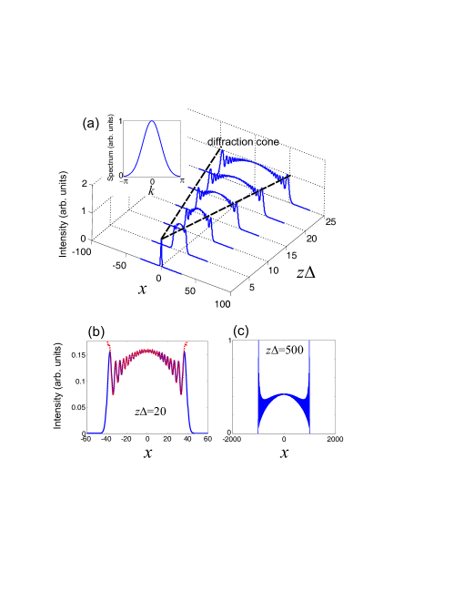
Figure 1: (color online) Beam propagation in a one-dimensional tight binding lattice with nearest neighboring coupling terms, showing far-field properties of discrete diffraction. In (a) the intensity distributions $|\psi(x,z)|^{2}$ are plotted, in arbitrary units, for propagation distances $z=0$, $z=5/\Delta$, $z=10/\Delta$, $z=15/\Delta$, $z=20/\Delta$, and $z=25/\Delta$, where $\Delta$ is the coupling rate between adjacent waveguides. The inset in (a) shows the Gaussian spectrum $F(k)$ of the beam ($w_{k}=1.5$). In (c) the intensity distribution $|\psi(x,z)|^{2}$ is depicted for a propagation distance $z=20/\Delta$ as numerically calculated by Eq.(27) (solid curve) and by the approximate relation (33) (dotted curve, almost overlapped with the solid one). In (c) the beam intensity is plotted at a propagation distance $z=500/\Delta$, clearly showing the dominance of two peaks at the diffraction cone edges (self-collimation directions) and the onset of three different decay laws at $|\alpha|>2\Delta$, $\alpha=\pm 2\Delta$, and $|\alpha|<2\Delta$.

as $z\rightarrow\infty$. From Eq.(31) we obtain the well-known result of paraxial diffraction theory that the amplitude $\psi_{0}(\alpha;z)$ of the beam decays as $\sim 1\sqrt{z}$ for any observation angle $\alpha$ note , and that the far-field diffraction pattern is shaped as the Fourier spectrum $F(\alpha)$ of the near-field distribution. This scaling law may be referred to as the normal scaling law, in the sense that the beam intensity $I\propto|\psi|^{2}$ decays as $\sim 1/z$ whereas the beam spot size $w_{x}$ increases asymptotically as $\sim z$ [see Eq.(17)], the product $Iw_{x}$ being constant according to the power conservation law.
For the discrete diffraction problem, we prove now that the decay law is generally slower than $\sim 1/\sqrt{z}$ at the observation angles corresponding to self-collimation, and that the far-field pattern is peaked at such angles and does not reproduce the spectrum $F$ of the near-field distribution. To this aim, let us observe that, according to the steepest descend method, the slowest decay term in the integral of Eq.(29) comes from the saddle points $g^{\prime}(k_{0})=0$ of largest order. In particular, if $k_{0}$ is a saddle point of order $n\geq 2$, i.e. $g(k)\simeq g(k_{0})+[g^{(n)}(k_{0})/n!](k-k_{0})^{n}$ for $k$ close to $k_{0}$ ($g^{(n)}(k_{0})\neq 0$), the contribution of the saddle point to the integral in Eq.(29) for large values of $z$ is given by Oliver74

$$\psi_{0}(\alpha;z)\sim\frac{F(k_{0})}{|zg^{(n)}(k_{0})|^{1/n}}(n!)^{\frac{1}{n}}\Gamma\left(\frac{1}{n}\right)\exp\left[izg(k_{0})\pm i\frac{\pi}{2n}\right].$$ (32)

Therefore, the decay law for $\psi_{0}(\alpha;z)$ scales as $\sim z^{-1/n}$, where $n$ is the highest order of the saddle points of $g(k)$, provided that $F(k_{0})\neq 0$. In the case of diffraction in a homogeneous continuous medium, the order of saddle point is always $n=2$. To determine $n$ for the discrete diffraction problem, let us note that the dispersion curve $H_{0}(k)$ admits of at least a couple of inflection points, say at $k=\pm k_{0}$, at which $H^{\prime\prime}_{0}(k_{0})=0$. These points correspond to the self-collimation directions introduced in Sec.II.C. Since $g^{\prime}(k)=\alpha-H^{\prime}_{0}(k)$, the inflection points $k=\pm k_{0}$ turn out to be also saddle points when the observation angle $\alpha$ is chosen equal to $H^{\prime}_{0}(\pm k_{0})$. Therefore, for the discrete diffraction problem the largest order $n$ of saddle points is at least $n=3$, and the decay law of $\psi_{0}(\alpha;z)$, at the two observation angles $\alpha=\pm H^{\prime}_{0}(k_{0})$ corresponding to the self-collimation directions $\pm k_{0}$, is slowed down -as compared to continuous diffraction- to (at least) $\sim z^{-1/3}$. More generally, if the dispersion curve $H_{0}(k)$ of the lattice is engineered to achieve a very flat behavior near a self-collimation point $k=k_{0}$, with $g^{\prime\prime}(k_{0})=g^{\prime\prime\prime}(k_{0})=...=g^{(n-1)}(k_{0})=0$ and $g^{(n)}(k_{0})\neq 0$ ($n\geq 3$), the decay law of $\psi_{0}(\alpha;z)$ scales as $\sim z^{-1/n}$ at the observation angle $\alpha=H^{\prime}(k_{0})$. This scaling law of beam decaying in the discrete diffraction problem is therefore anomalous, in the sense that along the self-collimation directions the intensity decays slower that $1/z$, i.e. of the characteristic decay law that one might expect from power conservation arguments. This seemingly paradoxical circumstance may be solved by observing that, for an observation angle $\alpha$ different than any of the self-collimation directions, the decay of $\psi_{0}(\alpha;z)$ may be either normal (i.e. $\sim 1/\sqrt{z}$) or even faster. More precisely, for a fixed value of $\alpha$ in modulus larger than $\alpha_{max}={\rm max}_{k}|H_{0}^{{}^{\prime}}(k)|$, the function $g(k)$ given by Eq.(30) does not have saddle points on the real axis, and $\psi_{0}(\alpha;z)$ decays as $\sim 1/z$. Conversely, for $|\alpha|<\alpha_{max}$ the equation $g^{\prime}(k)=\alpha-H_{0}^{{}^{\prime}}(k)=0$ admits of at least one solution, with $g^{\prime\prime}(k)\neq 0$ for a second-order saddle point. In this case, according to the method of stationary phase the asymptotic behavior of $\psi_{0}(\alpha;z)$ for large values of $z$ follows the normal law $\sim 1/\sqrt{z}$. To summarize, $\psi_{0}(\alpha;z)$ scales: as $\sim F(k_{0})z^{-1/n}$ at a self collimation direction $\alpha$, where $H_{0}^{{}^{\prime}}(k_{0})=\alpha$ and $k_{0}$ is a saddle point of order $n\geq 3$; as $\sim F(k_{0})z^{-1}$ for an observation angle $\alpha$ outside the ’diffraction cone’ $|\alpha|>\alpha_{max}$; as $\sim F(k_{0})z^{-1/2}$ inside the diffraction cone region $|\alpha|<\alpha_{max}$ but far from a self collimation direction. The far-field pattern of discrete diffraction tends therefore to confine light inside the diffraction cone $|\alpha|\leq\alpha_{max}$ with asymptotic peaks at the propagation directions corresponding to the angles of self-collimation.
This very general behavior may be illustrated more in details for the case of a tight-binding lattice in the nearest-neighbor approximation considered in Sec.II.C, for which $H_{0}(k)=-2\Delta\cos k$. In this lattice model one has $g^{\prime}(k)=\alpha-2\Delta\sin k$, $g^{\prime\prime}(k)=-2\Delta\cos k$, so that the angle of diffraction cone is given by $\alpha_{max}=2\Delta$. Two saddle points of second-order are found at $k=k_{0}=\pm\pi/2$ for the observation angles $\alpha=\pm\alpha_{max}$, i.e at the edge of the diffraction cone, at which the far-field discrete diffraction pattern is thus expected to show two peaks. For an observation angle $\alpha$ strictly inside the diffraction cone ($|\alpha|<2\Delta$), the equation $g^{\prime}(k)=0$ has two solutions which are saddle points of first order since $g^{\prime\prime}(k)\neq 0$. The main contribution to the integral on the right hand side of Eq.(29) comes from these two saddle points, and can be calculated by the method of stationary phase, yielding explicitly

$$\psi(\alpha;z) \sim \sqrt{\frac{i\pi}{z\sqrt{\Delta^{2}-(\alpha/2)^{2}}}}\left\{-iF(k_{0})\exp\left[i\alpha k_{0}z+2i\Delta z\cos k_{0}\right]+F(\pi-k_{0})\exp\left[i\alpha z(\pi-k_{0})-2i\Delta z\cos k_{0}\right]\right\}$$

$$(\alpha>0)$$

$$\psi(\alpha;z) \sim \sqrt{\frac{i\pi}{z\sqrt{\Delta^{2}-(\alpha/2)^{2}}}}\left\{-iF(-k_{0})\exp\left[-i\alpha k_{0}z+2i\Delta z\cos k_{0}\right]+F(-\pi+k_{0})\exp\left[i\alpha z(-\pi+k_{0})-2i\Delta z\cos k_{0}\right]\right\}$$ (33)

$$(\alpha<0)$$

where $k_{0}$ is the solution to the equation $\sin k_{0}=|\alpha/2\Delta|$ in the interval $0\leq k_{0}<\pi/2$. It should be noted that the far-field discrete diffraction pattern given by Eq.(33) holds for $|\alpha|<2\Delta$. As $|\alpha|$ approaches $2\Delta$ from below, the two saddle points of second order coalesce into a single saddle point of third order, and this explain the divergence of Eq.(33) as $|\alpha|\rightarrow 2\Delta$, i.e at the self collimation directions, where the decay is slower and scales as $\sim z^{-1/3}$. For $|\alpha|>2\Delta$, i.e. outside the diffraction cone, there are not saddle points on the real axis and the decay is faster and scales as $\sim 1/z$. An example of far-field discrete diffraction for a beam with a Gaussian spectrum $F(k)\sim\exp[-(k/w_{k})^{2}]$ ($-\pi\leq k<\pi$) is shown in Fig.1. In Fig.1(a) the intensity distribution $|\psi(x,z)|^{2}$, as obtained by accurate numerical computation of the integral entering in Eq.(27), is plotted for a few propagation distances $z$. For the sake of readability, at each propagation distance $z$ the field intensity has been normalized to its peak value. The diffraction cone and the emergence of two intensity peaks at the self-collimation directions $\alpha=\pm\alpha_{max}$ are clearly visible just after a propagation distance $z$ of $\sim 10-20$ times the coupling length $1/\Delta$ [Fig.1(a)]. Inside the diffraction cone, the intensity distribution at such propagation distances is very well fitted by the analytical far-field distribution given by Eq.(33), as shown in Fig.1(b). At much longer propagation distances, the self-collimation peaks become dominant, and the appearance of three different scaling laws of beam decay (fast decay outside the diffraction cone $|x|>2\Delta z$; normal decay inside the diffraction cone $|x|<2\Delta z$; slower decay at the self-collimation directions $x=\pm 2\Delta z$) is very clearly visible, as shown in Fig.1(c).

III Beam propagation in curved waveguide arrays

Discrete diffraction of light waves in linear optical waveguide arrays can be controlled by introducing transverse index gradients or local phase slips, which may produce a kind of refocusing or re-imaging of beam distributions along the propagation distances (see, for instance, Lenz99 ; Eisenberg00 ; Lenz03 ; Longhi05 ; SzameitAPL08 ) similarly to what happens to light propagating in continuous lensguide media. In particular, waveguide arrays with a curved axis provide a particularly interesting set up to manage discrete diffraction for both monochromatic and polychromatic light Lenz99 ; Lenz03 ; Longhi05 ; Garanovich06 ; Garanovich07 . It is therefore of major interest to have general laws describing the global behavior of beam propagation in curved waveguide arrays. In addition, it is well known that for the problem of paraxial diffraction in homogeneous continuous media or, more generally, of paraxial propagation in elementary optical systems and lensguides, one can introduce special families of field distributions (such as the Gaussian beams) that propagate maintaining unchanged their functional shape (shape-invariant beams), and that field propagation may be simply described by means of algebraic equations ruling out the evolution of some complex-valued beam parameters (such as the complex $q$-parameter for Gaussian beams; see, for instance, Siegman ). A natural question is whether one can similarly introduce shape-invariant discrete beams, i.e. field distributions that do not change their functional shape when propagating along curved waveguide arrays. As the problem of discrete diffraction in waveguide arrays with curved axis or transverselly-imposed index gradients is analogous to the problem of one-dimensional or two-dimensional Bloch oscillations of electrons in periodic potentials with an applied electric field or of cold atoms in optical lattices, some results are already available in the literature. In particular, in recent works B01 ; B02 ; B03 an algebraic approach has been developed, capable of providing rather general results for wave packet center of mass evolution and wave packet spreading in certain lattice models. In this approach, after the introduction of a dynamical Lie algebra, an explicit form of the evolution operator is first derived, and then the expectation values of operators are calculated in the Heisenberg picture. However, the question of existence of shape-invariant discrete beams and of their propagation in curved waveguide arrays does not seem to have been addressed yet. In this section, we present a generalization of Eqs.(12) and (17) describing the evolution of beam center of mass and beam width in curved waveguide arrays using the method of moments. Though similar results have been previously published in Refs.B01 ; B02 ; B03 using an algebraic operator approach, they are here re-derived for the sake of completeness using the method of moments, which does not require the explicit calculation of the evolution operator and the formulation of the problem in terms of a Lie algebra. In the subsequent section a family of shape-invariant discrete beams will be introduced, proving that their propagation in a generally-curved waveguide array is simply described by the evolution of a complex-$q$ beam parameter, which plays an analogous role of e.g. the complex-$q$ parameter of Gaussian beams propagating in paraxial continuous optical systems.
Let us consider monochromatic light propagation in a two-dimensional waveguide array with a curved axis described by the parametric equations $x=x_{0}(z)$ and $y=y_{0}(z)$; the coupled mode equations describing light transfer among coupled waveguides in the single-band and tight-binding approximations are an extension of Eq.(1) to include fictitious transverse index gradients induced by waveguide curvature and read explicitly

$$i\dot{c}_{n,m}=-\sum_{l,r}\Delta_{n-l,m-r}c_{l,r}-\mathcal{E}(z)\cdot\mathbf{r}_{n,m}$$ (34)

where $\mathcal{E}(t)=\mathcal{E}_{x}(t)\mathbf{u}_{x}+\mathcal{E}_{y}(t)\mathbf{u}_{y}$, $\mathcal{E}_{x}(z)=-(n_{s}/\lambdabar)\ddot{x}_{0}(z)$, $\mathcal{E}_{y}(z)=-(n_{s}/\lambdabar)\ddot{y}_{0}(z)$, $n_{s}$ is the refractive index of the waveguide substrate, and $\lambdabar=\lambda/(2\pi)$ is the reduced wavelength of light. It should be noticed that the transverse index gradient entering in Eq.(34) may be also realized by applying a thermal gradient, or may describe lumped phase gradients SzameitAPL08 or an abrupt tilt of waveguide axis direction Eisenberg00 , in which cases $\mathcal{E}(z)$ shows a delta-like behavior. After introduction of a continuous function $\psi(\mathbf{r},z)$ such that $\psi(\mathbf{r}_{n,m},z)=c_{n,m}(z)$, one can readily check that the discrete diffraction equations (34) are equivalent to the following continuous Hamiltonian problem

$$i\partial_{z}\psi(\mathbf{r},z)=H(\mathbf{r},\mathbf{p})\psi(\mathbf{r},z)$$ (35)

($\mathbf{p}=-i\nabla_{\mathbf{r}}$) with Hamiltonian

$$H=H_{0}(\mathbf{p})-\mathcal{E}(z)\cdot\mathbf{r},$$ (36)

where $H_{0}$ is the Hamiltonian of the homogeneous array defined by Eq.(3). The laws governing the evolution of beam center of mass and beam variance can be obtained by extending the method of moments described in Sec.II.B for the free diffraction problem. In general, the cascade of equations that one obtains by applying the Eherenfest equation (9) to $\langle\mathbf{r}\rangle$, $\langle x^{2}\rangle$, $\langle y^{2}\rangle$ - and to the commutators found throughout the calculations- turns out to be unlimited for a general form of $H_{0}$, and a closed set of equations are found solely for special forms of $H_{0}$. Such a special circumstance is encountered in case of a one-dimensional waveguide array in the nearest-neighboring approximation, and in case of a rectangular-lattice waveguide array neglecting diagonal interactions. The first model corresponds to the Hamiltonian

$$H(x,p)=-2\Delta\cos p-\mathcal{E}_{x}(z)x,$$ (37)

where $\Delta$ is the coupling rate between adjacent waveguides, and $p=p_{x}=-i\partial_{x}$. The second model, which has been for instance considered in the experiment of Ref.Pertsch04 , is described by the Hamiltonian

$$H(\mathbf{r},\mathbf{p})=-2\Delta_{x}\cos(p_{x})-2\Delta_{y}\cos(p_{y})-\mathcal{E}_{x}(t)x-\mathcal{E}_{y}(z)y,$$ (38)

where $\Delta_{x}$ ($\Delta_{y}$) is the coupling rate between adjacent horizontal (vertical) waveguides of the lattice notaS .

III.1 One-dimensional array

Application of the moment method to the one-dimensional Hamiltonian model (37) yields a set of closed coupled equations for the expectation values of operators $x$, $\theta$, and of $x^{2}$, $\rho$ and $\sigma$, where

$$\theta = \exp(ip)$$ (39)

$$\rho = \frac{1}{2}\left\{1-\exp(-2ip)\right\}$$ (40)

$$\sigma = i\left\{x\exp(-ip)+\exp(-ip)x\right\}.$$ (41)

Successive application of the Ehrenfest equation (9) yields the following equations for $\langle x\rangle$ and $\langle\theta\rangle$

$$\frac{d\langle x\rangle}{dz} = 2\Delta{\rm Im}\left(\langle\theta\rangle\right)$$ (42)

$$\frac{d\langle\theta\rangle}{dz} = i\mathcal{E}_{x}(z)\langle\theta\rangle,$$ (43)

and the following coupled equations for $\langle x^{2}\rangle$, $\langle\rho\rangle$ and $\langle\sigma\rangle$

$$\frac{d\langle x^{2}\rangle}{dz} = 2\Delta{\rm Re}\left(\langle\sigma\rangle\right)$$ (44)

$$\frac{d\langle\rho\rangle}{dz} = -2i\mathcal{E}_{x}(z)\langle\rho\rangle+i\mathcal{E}_{x}(z)$$ (45)

$$\frac{d\langle\sigma\rangle}{dz} = 4\Delta\langle\rho\rangle-i\mathcal{E}_{x}(z)\langle\sigma\rangle.$$ (46)

Equation (43) can be readily integrated, yielding the following evolution equation for the beam center of mass

$$\langle x(z)\rangle=\langle x(0)\rangle+2{\rm Im}\left\{q_{0}\Omega^{*}(z)\right\}$$ (47)

where we have set

$$\Omega(z) \equiv \int_{0}^{z}d\xi\Delta\exp[-i\phi(\xi)],$$ (48)

$$\phi(z) \equiv \int_{0}^{z}d\xi\mathcal{E}_{x}(\xi),$$ (49)

$$q_{0} \equiv \sum_{n}c_{n}^{*}(0)c_{n+1}(0).$$ (50)

Similarly, integration of Eqs.(45) and (46) yields

$$\langle\rho(z)\rangle=\exp[-2i\phi(z)]\times$$

$$\times\left\{\langle\rho(0)\rangle+\frac{1}{2}\exp[2i\phi(z)]-\frac{1}{2}\right\}$$ (51)

$$\ \langle\sigma(z)\rangle=\exp[-i\phi(z)]\times$$

$$\times\left\{\langle\sigma(0)\rangle+4\Omega(z)\left[\langle\rho(0)\rangle-\frac{1}{2}\right]+2\Omega^{*}(z)\right\}$$ (52)

Taking into account that $\Delta\exp[-i\phi(z)]=d\Omega/dz$ and that $2{\rm Re}\left\{\int_{0}^{z}d\xi\Omega^{*}(\xi)(d\Omega/d\xi)\right\}=|\Omega(z)|^{2}$, substitution of Eq.(52) into Eq.(44) yields

$$\langle x^{2}(z)\rangle=\langle x^{2}(0)\rangle+2|\Omega(z)|^{2}+2{\rm Re}\left\{q_{1}\Omega(z)-q_{2}\Omega^{2}(z)\right\},$$ (53)

where we have set

$$q_{1} \equiv i\sum_{n}(2n-1)c^{*}_{n}(0)c_{n-1}(0)$$ (54)

$$q_{2} \equiv \sum_{n}c^{*}_{n}(0)c_{n-2}(0).$$ (55)

The beam size $w_{x}$ is then given by

$$w_{x}(z)=\sqrt{\langle x^{2}(z)\rangle-\langle x(z)\rangle^{2}}.$$ (56)

For a given field distribution $c_{n}(0)$ at the input plane, the evolution of the beam center of mass $\langle x(z)\rangle$ and beam size $w_{x}(z)$ are thus ruled by Eqs.(47), (53) and (56). Note that beam evolution depend on the input beam parameters $q_{1}$, $q_{2}$ and $q_{3}$ -defined by Eqs.(50),(54) and (55)- and by the complex amplitude $\Omega(z)$, defined by Eqs.(48-49) and accounting for bending of waveguide axis. Note also that for straight arrays $\Omega(z)=\Delta z$, and one thus retrieves the results of discrete diffraction derived in Sec.II.B, in particular the linear asymptotic increase of $w_{x}$ with $z$. The condition for diffraction suppression, i.e. a non-secular growth of $w_{x}(z)$ with $z$, is that $\Omega(z)$ remains a limited function of $z$ as $z$ increases. This condition is always satisfied for a constant value of $\mathcal{E}_{x}$, which corresponds to circularly-curved waveguides and to the onset of the optical analogue of Bloch oscillations Lenz99 . Similarly, for periodic axis bending with spatial period $\Lambda$, $\mathcal{E}_{x}(z)$ is a periodic function of $z$, and the condition of boundness of $\Omega(z)$ is given by

$$\int_{0}^{\Lambda}d\xi\exp[-i\phi(\xi)]=0,$$ (57)

which is precisely the condition of ’dynamic localization’ previously investigated in Refs.Lenz03 ; Longhi05 .

III.2 Two-dimensional array

For the two-dimensional waveguide array model (38), the moment equations turn out to decouple into two set of equations, similar to Eqs.(42-46), separately acting onto the $x$ and $y$ directions. The evolution equations for the beam center of mass $\langle x\rangle$, $\langle y\rangle$ are then given by

$$\langle x(z)\rangle = \langle x(0)\rangle+2{\rm Im}\left\{q_{0x}\Omega_{x}^{*}(z)\right\}$$ (58)

$$\langle y(z)\rangle = \langle y(0)\rangle+2{\rm Im}\left\{q_{0y}\Omega_{y}^{*}(z)\right\}$$ (59)

where we have set

$$\Omega_{x,y}(z) = \int_{0}^{z}d\xi\Delta_{x,y}\exp[-i\phi_{x,y}(\xi)]$$ (60)

$$\phi_{x,y}(z) = \int_{0}^{z}d\xi\mathcal{E}_{x,y}(\xi)$$ (61)

and

$$q_{0x} = \sum_{n,m}c^{*}_{n,m}(0)c_{n+1,m}(0)$$ (62)

$$q_{0y} = \sum_{n,m}c^{*}_{n,m}(0)c_{n,m+1}(0).$$ (63)

Similarly, the beam sizes $w_{x}$ and $w_{y}$, defined as

$$w_{x}(z) = \sqrt{\langle x^{2}(z)\rangle-\langle x(z)\rangle^{2}}$$ (64)

$$w_{y}(z) = \sqrt{\langle y^{2}(z)\rangle-\langle y(z)\rangle^{2}},$$ (65)

are calculated using Eqs.(58-59) and the following evolution equations for $\langle x^{2}(z)\rangle$ and $\langle y^{2}(z)\rangle$

$$\langle x^{2}(z)\rangle=\langle x^{2}(0)\rangle+2|\Omega_{x}|^{2}+2{\rm Re}\left\{q_{1x}\Omega_{x}-q_{2x}\Omega_{x}^{2}\right\}$$ (66)

$$\langle y^{2}(z)\rangle=\langle y^{2}(0)\rangle+2|\Omega_{y}|^{2}+2{\rm Re}\left\{q_{1y}\Omega_{y}-q_{2y}\Omega_{y}^{2}\right\}$$ (67)

where we have set

$$q_{1x} = i\sum_{n,m}(2n-1)c^{*}_{n,m}(0)c_{n-1,m}(0)$$ (68)

$$q_{2x} = \sum_{n,m}c^{*}_{n,m}(0)c_{n-2,m}(0)$$ (69)

$$q_{1y} = i\sum_{n,m}(2m-1)c^{*}_{n,m}(0)c_{n,m-1}(0)$$ (70)

$$q_{2y} = \sum_{n,m}c^{*}_{n,m}(0)c_{n,m-2}(0).$$ (71)

IV Shape-invariant discrete beams

The existence of shape-invariant beams, i.e. families of field distributions that propagate without changing their functional shape, is well-known for paraxial propagation in Gaussian optics or in continuous lensguide media (see, for instance, Siegman ). Here we address the related problem of investigating the existence of shape-invariant discrete beams, i.e. field distributions that do not change their functional shape when propagating along waveguide arrays with arbitrarily curved optical axis. This is a rather challenging problem because no general method capable of constructing shape-invariant beams seems to be available. However, for the simple waveguide array models considered in the previous section, a family of shape-invariant discrete beams can be introduced in a simple manner. Owing to their functional form, such beams are referred to as discrete Bessel beams.

IV.1 Discrete Bessel beams in one-dimensional arrays

Let us consider a one-dimensional waveguide array with an arbitrarily curved optical axis. In the tight-binding and nearest neighboring coupling approximations, light propagation is described by the following set of coupled-mode equations

$$i\dot{c}_{n}=-\Delta(c_{n+1}+c_{n-1})-nf(z)c_{n}$$ (72)

where $f(z)$ describes the rate of transverse index gradient induced by waveguide bending Longhi05 , lumped waveguide tilting Eisenberg00 or locally imposed phase changes among adjacent waveguides SzameitAPL08 as discussed previously. Let us fist observe that, if $c_{n}(z)$ is a solution to Eq.(72) corresponding to a given initial field distribution $c_{n}(0)$, then for an arbitrary integer $n_{0}$

$$g_{n}(z)=c_{n-n_{0}}(z)\exp\left\{in_{0}\int_{0}^{z}d\xi f(\xi)\right\}$$ (73)

is the solution to Eq.(72) corresponding to the translated initial field distribution $g_{n}(0)=c_{n-n_{0}}(0)$. Therefore, apart from an unimportant phase change, shape-invariant beams remain invariant for an arbitrary transverse translation on the lattice.
Let us tentatively search for a solution to Eq.(72) of the form

$$c_{n}(z)=J_{n}(\alpha)\exp(-i\sigma n)$$ (74)

where $J_{n}$ is the Bessel function of first kind of order $n$, and $\alpha=\alpha(z)$, $\sigma=\sigma(z)$ are unknown functions which depend on propagation distance $z$, but not on lattice site $n$. Note that, as $\sum_{n}n|J_{n}(\alpha)|^{2}=0$ and $[\sum_{n}|J_{n}(\alpha)|^{2}n^{2}]=\alpha^{2}/2$, the parameter $\alpha$ is related to the beam size $w_{x}$ [Eq.(6)] by the simple relation $w_{x}=\alpha/{\sqrt{2}}$, whereas $\sigma$ defines a transverse tilt of the beam ’phase front’. Substitution of Eq.(74) into Eq.(72) and taking into account the identities of Bessel functions $J_{n+1}(\alpha)+J_{n-1}(\alpha)=(2n/\alpha)J_{n}(\alpha)$ and $J_{n-1}(\alpha)-J_{n+1}(\alpha)=2J^{\prime}_{n}(\alpha)$, one obtains that Eq.(74) is indeed a solution to Eq.(72) provided that $\alpha$ and $\sigma$ satisfy the coupled equations

$$\dot{\alpha} = -2\Delta\sin\sigma$$ (75)

$$\dot{\sigma} = -\frac{2\Delta}{\alpha}\cos\sigma-f.$$ (76)

Owing to the functional form of $c_{n}$, we will refer such shape-invariant beams to as discrete Bessel beams. Let us define a complex-$q$ parameter for the discrete Bessel beam (74) according to

$$q(z)=\alpha(z)\exp[i\sigma(z)]$$ (77)

so that the modulus of the complex $q$ parameter gives the beam spot size at propagation distance $z$, whereas its phase corresponds to the phase front gradient. From Eqs.(75) and (76) one readily obtains for the complex $q$ parameter the following simple evolution equation

$$\frac{dq}{dz}=-2i\Delta-if(z)q.$$ (78)

The general solution to Eq.(78), for a given initial value $q(0)$ at the $z=0$ input plane, is given by

$$q(z)=\exp[-i\phi(z)]\left\{q(0)-2i\int_{0}^{z}d\xi\Delta\exp[i\phi(\xi)]\right\}$$ (79)

where

$$\phi(z)=\int_{0}^{z}d\xi f(\xi).$$ (80)

The propagation of a discrete Bessel beam along a curved waveguide array is thus reduced to the propagation of its complex $q$ parameter, which plays an analogous role of the complex-$q$ parameter for Gaussian beams in lensguide media. The propagation law of the $q$ parameter admits of a simple geometrical interpretation in the complex $q$ plane. According to Eq.(78), for an infinitesimal propagation distance $\delta z$ the change of $q(z)$ is given by the superposition of the two paths AB and BC shown in Fig.2(a). The path AB, of length $2\delta z\Delta$, accounts for discrete diffraction and corresponds to a change of $q(z)$ along the imaginary $q$ axis; the path BC is due to the transverse index gradient which produces a clockwise rotation by the angle $\delta\gamma=f(z)\delta z$ around the origin O of the complex plane. It is interesting to note that, since $J_{n}(0)=\delta_{n,0}$, for $q(0)=0$ the discrete Bessel beam (74) reduces to the well-known impulse response of a tight-binding array with nearest neighbor couplings (see, for instance, Dunlap86 ).
To appreciate the usefulness of the $q$-parameter description and some properties of discrete Bessel beams, let us now discuss a few examples and applications.

Figure 2: (a) Geometric construction of the evolution of the complex $q$ parameter for an infinitesimal propagation distance $\delta z$. The length of the segment AB is $2\Delta\delta z$, whereas the rotation angle is $\delta\gamma=f(z)\delta z$. The points $A$ and $C$ correspond to $q(z)$ and $q(z+\delta z)$, respectively. (b) Geometric representation of a self-imaging array: the path followed by the complex parameter $q(z)$, starting from the origin $O$, is closed.

Propagation of discrete Bessel beams in homogeneous arrays.
For a homogeneous array ($f=0$), the propagation law of the complex-$q$ parameter is simply given by

$$q(z)=q(0)-2i\Delta z.$$ (81)

If we assume, for the sake of definiteness, that at the input plane $z=0$ the phase front of the beam is flat, i.e. $q(0)=\alpha(0)=\alpha_{0}$ real valued, the following propagation laws for beam size $\alpha$ and beam phase tilt $\sigma$ are derived

$$\alpha(z) = \alpha_{0}\sqrt{1+\left(\frac{2\Delta z}{\alpha_{0}}\right)^{2}}$$ (82)

$$\sigma(z) = -{\rm arctan}\left(\frac{2\Delta z}{\alpha_{0}}\right).$$ (83)

From Eq.(82) we may introduce, as for Gaussian beams propagating in free space Siegman , the Rayleigh range $z_{R}$ and divergence angle $\theta_{d}$ such that $\alpha(z_{R})=\sqrt{2}\alpha_{0}$ and $\theta_{d}=\lim_{z\rightarrow\infty}\alpha(z)/z$, i.e.

$$z_{R} = \frac{\alpha_{0}}{2\Delta}$$ (84)

$$\theta_{d} = 2\Delta.$$ (85)

It should be noted that, as opposed to the case of Gaussian beams in free space -for which the Rayleigh range $z_{R}$ is proportional to the square of the spot size $\alpha_{0}$ at the beam waist and the diffraction angle $\theta_{d}$ is inversely proportional to $\alpha_{0}$- for discrete Bessel beams the Rayleigh range $z_{R}$ is proportional to the spot size $\alpha_{0}$ at the beam waist whereas the divergence angle is independent of the beam spot size and always equal to the diffraction cone angle introduced in Sec.II.D. This peculiar property is closely related to the very general result, proven in Sec.II.D, that the far field of discrete diffraction in a homogenous waveguide array is peaked at the observation angles corresponding to the flattest points (self-collimation points) of the band dispersion curve.

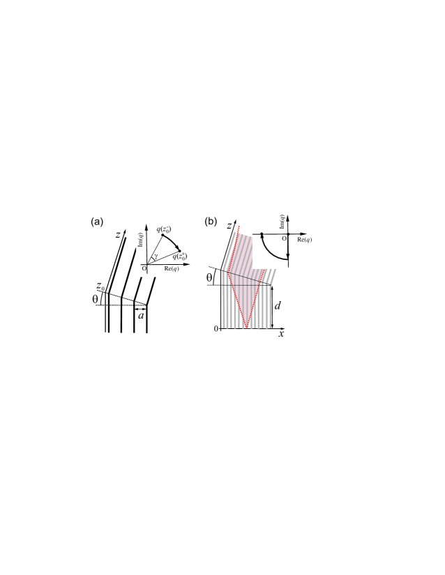
Figure 3: (color online) (a) Schematic of a one-dimensional waveguide array with a tilt of waveguide axis at $z=z_{0}$, and the transformation induced on the complex $q$ parameter by the tilt (inset). (b) Principle of beam collimation via waveguide axis tilt [tilt angle $\theta=\lambda/(4an_{s})$], and path followed by the complex $q$ parameter for single waveguide input excitation from $z=0$ to $z=d^{+}$ (inset).

Transformation of a discrete Bessel beam through a waveguide axis tilt. A tilt of the waveguide axis at $z=z_{0}$ by a (small) angle $\theta$ corresponds to impressing a phase shift

$$\gamma=\frac{2\pi}{\lambda}a\theta n_{s}$$ (86)

between adjacent waveguides, where $a$ is the waveguide spacing and $n_{s}$ the effective index of propagating modes [see Fig.3(a)]. Light propagation across the tilt can be thus modelled by assuming $f(z)=\gamma\delta(z-z_{0})$ in Eq.(72), and its effect on the complex $q$ parameter is to produce a rotation around the origin of the complex plane by an angle $\gamma$ [see the inset of Fig.3(a)].
A tilt of the waveguide axis may be used to ’collimate’ a discrete beam, as schematically shown in Fig.3(b). Here a single waveguide is initially excited at the input plane, and after a propagation distance $d$ the axis of the array is tilted by an angle $\theta=\lambda/(4an_{s})$ such that $\gamma=\pi/2$. The 90^o rotation of the $q$ parameter in the complex plane due to axis bending [see the inset in Fig.3(b)] brings the $q$ parameter on the real axis, with a zero phase gradient $\sigma=0$ and an enlarged beam size $\alpha=2\Delta d$. The axis tilt thus plays a similar role of a collimating lens for a diverging Gaussian beam. Note however that, contrary to a conventional lens, the tilting angle $\theta$ to achieve beam collimation is independent of the distance $d$ between source point (at $z=0$) and the lens plane ($z=d$). Figure 4 shows an example of beam collimation in a 6-cm-long one-dimensional array as obtained by numerical analysis of the scalar wave equation for the electric field envelope $E(x,z)$ propagating in the structure based on a standard beam propagation method. Figure 4(a) shows a pseudocolor map of the intensity beam evolution $|E(x,z)|^{2}$ along the structure when a single waveguide is excited in its fundamental mode at the input plane $z=0$ and the waveguide axis is tilted at a distance $d=2$ cm from the input plane [horizontal dotted curve in Fig.4(a)]. The refractive index profile $n(x)$ used in the simulations is depicted in Fig.4(b), and the values of other parameters are $\lambda=1.55\;\mu$m, $n_{s}=1.52$, and $a=11\;\mu$m, corresponding to a tilting angle $\theta=\lambda/(4an_{s})\simeq 23.2\;{\rm mrad}$. For the sake of readability, the intensity distribution is plotted with the waveguide axis $z$ unfolded along a straight line. Note that the numerical results provide a realistic behavior of beam propagation beyond the couple-mode equation approximation, accounting for radiation losses and coupling to higher-order bands due to axis bending. These latter effects, however, are very small for the parameter values adopted in the simulations, and the coupled-mode equation model works fine.

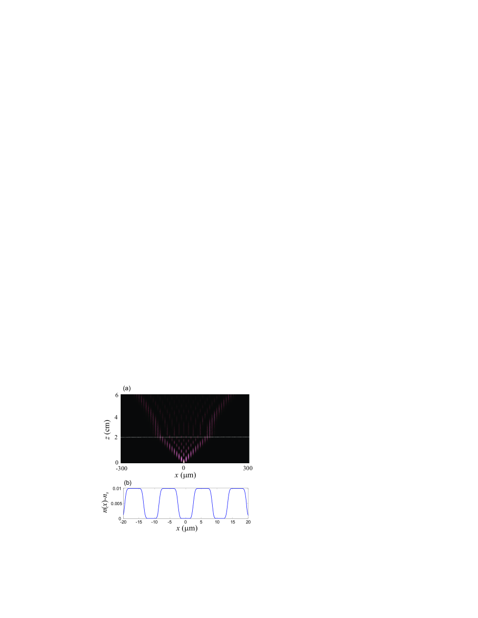
Figure 4: (color online) (a) Pseudocolor map of beam intensity propagation in a waveguide array with one axis tilting as obtained by numerical simulations, showing beam collimation. (b) Refractive index profile of the waveguide array used in the numerical simulations. The values of other parameters are given in the text.

A geometric interpretation of the self-imaging condition and polygonal Bloch oscillations. An array of length $d$ shows a self-imaging property (also referred to as diffraction cancellation or dynamic localization) , whenever $|c_{n}(d)|^{2}=|c_{n}(0)|^{2}$ for any initial field distribution. The dynamic localization condition has a rather simple geometric interpretation in the complex $q$ plane. In fact, if the array is excited in waveguide $n=0$, $q(0)=0$ and to achieve self-imaging after a propagation distance $d$ one has necessarily to have $q(d)=q(0)=0$, i.e the path described by the complex $q$ parameter, starting from the origin O of the complex plane, should be closed [see Fig.2(b)]. Owing to the translational invariance of discrete Bessel beams [Eq.(73)], this condition is also sufficient. From Eq.(79), the closed-path condition $q(d)=q(0)=0$ yields

$$\int_{0}^{d}dz\exp[i\phi(z)]=0$$ (87)

which is precisely the condition for dynamic localization derived originally by Dunlap and Kenkre in Ref.Dunlap86 .
An application of the geometric condition of dynamic localization is that of polygonal Bloch oscillations. Let us consider a waveguide array whose axis forms an (open) polygonal curve of large (mean) radius $R$ made of a sequence of straight segments of same length $b$ and with tilt angle $\theta$, as shown in Fig.5(a). The function $\phi(z)$, defined by Eq.(80), is thus a staircase function, which increases in steps of $\gamma=(2\pi/\lambda)a\theta n_{s}$ [see Eq.(86)] at $z=b,2b,3b,...$ (the coordinate $z$ is measured along the polygonal curve). After a propagation $d=(N+1)b$ from the input $z=0$ plane, where $N$ is an integer number, it then follows that

$$\int_{0}^{d}dz\exp[i\phi(z)]=b\sum_{n=0}^{N}\exp(i\gamma n).$$ (88)

The sum of complex numbers (phasors) on the right hand side of Eq.(88) can be done analytically and has a well-known geometric interpretation; in particular, if $\gamma$ satisfies the condition $\gamma=2\pi/(N+1)$, i.e. if the tilt angle $\theta$ is given by

$$\theta=\frac{\lambda}{an_{s}(N+1)}$$ (89)

the sum on the right hand side of Eq.(88) vanishes, and the condition for self-imaging is attained. An example of the self-imaging property of a polygonal waveguide array is shown in Fig.5(b) for the case $N=5$. The figure depicts a characteristic breathing mode corresponding to a single waveguide excitation at the input plane. The waveguide array parameters are the same as in Fig.4, and a sequence of axis tilts are placed at distances $b=1$ cm one to the next. The tilt angle $\theta$, chosen according to Eq.(89), is $\theta\simeq 15.5\;{\rm mrad}$, yielding a self-imaging plane at $d=(N+1)b=6\;{\rm cm}$, as clearly shown in Fig.5(b). Note that, in the limit $b\rightarrow 0$, $N\rightarrow\infty$ and $b/\theta\rightarrow R$ finite, the polygonal of Fig.5(a) approximates an arc of a circumference of radius $R$, and the condition (89) for self-imaging is satisfied for a propagation distance

$$d=(N+1)b\rightarrow\frac{\lambda R}{n_{s}a}$$ (90)

which is the spatial period of Bloch oscillations on a curved waveguide array (radius of curvature $R$) previously considered in Refs.Lenz99 ; Usievich04 . The usual Bloch oscillations on a curved waveguide array may be therefore viewed as a limiting case of Bloch oscillations on a polygonal array.

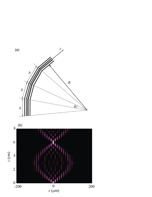
Figure 5: (color online) (a) Schematic of a polygonal waveguide array for the observation of Bloch oscillations. (b) Pseudocolor image of beam intensity propagation in a 8-cm-long polygonal array showing a Bloch oscillation breathing mode. The refractive index profile of the waveguide array used in the numerical simulations is the same as in Fig.4(b). The values of other parameters are given in the text.

IV.2 Discrete Bessel beams in two-dimensional arrays

A simple extension of the analysis of Sec.IV.A can be done for a two-dimensional rectangular-lattice waveguide array with nearest-neighboring coupling when the diagonal coupling is neglected. This model is described by the coupled mode equations

$$i\dot{c}_{n,m} = -\Delta_{x}(c_{n+1,m}+c_{n-1,m})-\Delta_{y}(c_{n,m+1}+c_{n,m-1})$$ (91)

$$- f_{x}(z)nc_{n,m}-f_{y}(z)mc_{n,m}$$

where $f_{x,y}(z)$ describe the rates of transverse index gradients induced by waveguide bending or lumped waveguide axis tilting along the $x$ and $y$ directions. Since Eqs. (91) admit of separable solutions $c_{n,m}(z)=c_{n}(z)c_{m}(z)$, with $c_{n}(z)$ and $c_{m}(z)$ solutions to the one-dimensional problem (72) with $\Delta=\Delta_{x,y}$ and $f(z)=f_{x,y}(z)$, a two-dimensional discrete Bessel beam has the form

$$c_{n,m}(z)=J_{n}(\alpha_{x})J_{m}(\alpha_{y})\exp(-i\sigma_{x}n-\sigma_{y}m).$$ (92)

The complex-$q$ parameters of the beam along the $x$ and $y$ directions are defined by

$$q_{x}(z)=\alpha_{x}(z)\exp[i\sigma_{x}(z)]\;,\;q_{y}(z)=\alpha_{y}(z)\exp[i\sigma_{y}(z)]$$ (93)

and their evolution is ruled out by the equations

$$\dot{q}_{x,y}=-2i\Delta_{x,y}-if_{x,y}(z)$$ (94)

which have a similar geometric interpretation as that discussed in Sec.IV.A. The propagation properties of two-dimensional discrete Bessel beams in homogeneous arrays, across tilted axis regions or polygonal curves are the same as those investigated for one-dimensional beams, and are therefore not further discussed here.

V Conclusions

In this work, a comprehensive study of discrete diffraction and linear propagation of light in homogeneous and curved waveguide arrays has been presented. In particular, general laws describing beam spreading, beam decay and discrete far-field patterns in homogeneous arrays have been derived using the method of moments and the steepest descend method, and some remarks on the well-known self-collimation regime have been pointed out. In curved arrays and within the nearest neighboring coupling approximation, the method of moments has been extended to describe the evolution of global beam parameters. This method provides an alternative means to algebraic operator techniques recently proposed in other physical contexts to study general properties of Bloch oscillations B01 ; B02 ; B03 . Finally, a family of shape-invariant discrete beams -referred to as discrete Bessel beams owing to their functional form- has been introduced. It has been shown that propagation of such beams in curved waveguide arrays is simply described by the evolution of a complex $q$ parameter, which plays a similar role to the complex $q$ parameter used for Gaussian beams in continuous lensguide media. A few applications of the $q$ parameter formalism are discussed, including beam collimation via waveguide axis tilting, a geometric interpretation of the self-imaging effect in waveguide arrays, and optical Bloch oscillations on a polygonal array.

References

- (1) D. N. Christodoulides, F. Lederer, and Y. Silberberg, Nature 424, 817 (2003).
- (2) F. Lederer, G.I. Stegeman, D.N. Christodoulides, G. Assanto, M. Segev, and Y. Silberberg, Phys. Rep. 463, 1 (2008).
- (3) H. S. Eisenberg, Y. Silberberg, R. Morandotti, J. S. Aitchison, Phys. Rev. Lett. 85, 1863 (2000) .
- (4) T. Pertsch, T. Zentgraf, U. Peschel, A. Bräuer, and F. Lederer, Phys. Rev. Lett. 88, 093901 (2002).
- (5) R. Iwanow, D.A. May-Arrioja, D.N. Christodoulides, G.I. Stegeman, Y. Min, and W. Sohler, Phys. Rev. Lett. 95, 053902 (2005).
- (6) A. Szameit, F. Dreisow, H. Hartung, S. Nolte, A. Tünnermann and F. Lederer, Appl. Phys. Lett. 90, 241113 (2007).
- (7) U. Peschel, T. Pertsch, and F. Lederer, Opt. Lett. 23, 1701 (1998).
- (8) R. Morandotti, U. Peschel, J. S. Aitchison, H. S. Eisenberg, and Y. Silberberg, Phys. Rev. Lett. 83, 4756 (1999); T. Pertsch, P. Dannberg, W. Elflein, A. Bräuer, and F. Lederer, Phys. Rev. Lett. 83, 4752 (1999).
- (9) G. Lenz, I. Talanina, and C.M. de Sterke, Phys. Rev. Lett. 83, 963 (1999).
- (10) B.A. Usievich, V.A. Sychugov, J.Kh. Nirligareev, and K.M. Golant, Opt. Spectrosc. 97, 790 (2004); N. Chiodo, G. DellaValle, R. Osellame, S. Longhi, G. Cerullo, R. Ramponi, P. Laporta, and U. Morgner, Opt. Lett. 31, 1651 (2006); H. Trompeter, T. Pertsch, F. Lederer, D. Michaelis, U. Streppel, A. Bräuer, and U. Peschel, Phys. Rev. Lett. 96, 023901 (2006); H. Trompeter, W. Krolikowski, D. N. Neshev, A. S. Desyatnikov, A. A. Sukhorukov, Yu. S. Kivshar, T. Pertsch, U. Peschel, and F. Lederer, Phys. Rev. Lett. 96, 053903 (2006).
- (11) A. Szameit, T. Pertsch, S. Nolte, A. Tünnermann, U. Peschel, and F. Lederer, J. Opt. Soc. Am. B 24, 2632 (2007).
- (12) G. Lenz, R. Parker, M. C. Wanke, and C. M. Sterke, Opt. Commun. 218, 87 (2003); J. Wan, M. Laforest, C. M. de Sterke, and M.M. Dignam, Opt. Commun. 247, 353 (2005).
- (13) S. Longhi, Opt. Lett. 30, 2137 (2005); S. Longhi, M. Marangoni, M. Lobino, R. Ramponi, P. Laporta, E. Cianci, and V. Foglietti, Phys. Rev. Lett. 96, 243901 (2006); S. Longhi, M. Lobino, M. Marangoni, R. Ramponi, P. Laporta, E. Cianci, and V. Foglietti, Phys. Rev. B 74, 155116 (2006); R. Iyer, J. S. Aitchison, J. Wan, M. M. Dignam, and C. M. de Sterke, Opt. Express 15, 3212 (2007); F. Dreisow, M. Heinrich, A. Szameit, S. Döring, S. Nolte, A. Tünnermann, S. Fahr, and F. Lederer, Opt. Express 16, 3474 (2008).
- (14) I.L. Garanovich, A.A. Sukhorukov, and Y.S. Kivshar, Phys. Rev. E 74, 066609 (2006); I. L. Garanovich, A.A. Sukhorukov, and Y.S. Kivshar, Opt. Express 15, 9547 (2007); I.L. Garanovich, Phys. Lett. A 372, 3922 (2008).
- (15) I.L. Garanovich, A. Szameit, A.A. Sukhorukov, T. Pertsch, W. Krolikowski, S. Nolte, D. Neshev, A. Tünnermann, and Y. S. Kivshar, Opt. Express 15, 9737 (2007).
- (16) M.J. Ablowitz and Z.H. Musslimani, Phys. Rev. Lett. 87, 254102 (2001); I.L. Garanovich, A.A. Sukhorukov, and Yu. S. Kivshar, Opt. Express 15, 9547 (2007); A. Szameit, I.L. Garanovich, M. Heinrich, A. Minovich, F. Dreisow, A.A. Sukhorukov, T. Pertsch, D.N. Neshev, S. Nolte, W. Krolikowski, A. Tünnermann, A. Mitchell, and Y.S. Kivshar, Phys. Rev. A 78, 031801(R) (2008).
- (17) K.G. Makris and D.N. Christodoulides, Phys. Rev. E 73, 036616 (2006); S. Longhi, Phys. Rev. E 74, 026602 (2006); A. Szameit, T. Pertsch, F. Dreisow, S. Nolte, A. Tünnermann, U. Peschel, and F. Lederer, Phys. Rev. A 75, 053814 (2007).
- (18) R. Iwanow, R. Schiek, G.I. Stegeman, T. Pertsch, F. Lederer, Y. Min, and W. Sohler, Phys. Rev. Lett. 93, 113902 (2004); S. Suntsov, K.G. Makris, D.N. Christodoulides, G.I. Stegeman, A. Hache, R. Morandotti, H. Yang, G. Salamo, and M. Sorel, Phys. Rev. Lett. 96, 063901 (2006); Y.V. Kartashov, L. Torner, and V.A. Vysloukh, Phys. Rev. Lett. 96, 073901 (2006); M. Molina, Y. Kartashov, L. Torner, and Y. Kivshar, Opt. Lett. 32, 2668 (2007); A. Szameit, Y.V. Kartashov, F. Dreisow, T. Pertsch, S. Nolte, A. Tünnermann, and L. Torner, Phys. Rev. Lett. 98, 173903 (2007); X. Wang, A. Bezryadina, Z. Chen, K.G. Makris, D.N. Christodoulides, and G.I. Stegeman, Phys. Rev. Lett. 98, 123903 (2007).
- (19) I.L. Garanovich, A.A. Sukhorukov, and Y. S. Kivshar, Phys. Rev. Lett. 100, 203904 (2008); A. Szameit, I.L. Garanovich, M. Heinrich, A.A. Sukhorukov, F. Dreisow, T. Pertsch, S. Nolte, A. Tünnermann, and Yu. S. Kivshar, Phys. Rev. Lett. 101, 203902 (2008).
- (20) H. Kosaka, T. Kawashima, A. Tomita, M. Notomi, T. Tamamura, T. Sato, S. Kawakami, Appl. Phys. Lett. 74, 1212 (1999) ; J. Witzens, M. Loncar, A. Scherer, IEEE J. Sel. Topics Quantum Electron. 8, 1246 (2002) ; Z. Lu, S. Shi, J.A. Murakowski, G.J. Schneider, C.A. Schuetz, D.W. Prather, Phys. Rev. Lett. 96, 173902 (2006); P. T. Rakich, M. S. Dahlem, S. Tandon, M. Ibanescu, M. Soljacic, G. S. Petrich, J. D. Joannopoulos, L. A. Kolodziejski, E. P. Ippen, Nat. Mater. bf 5, 93 (2006).
- (21) See, for instance: J. M. Ziman, Principles of the Theory of Solids (second edition, Cambridge University Press, Cambridge, 1979).
- (22) S.G. Krivoshlykov,Quantum-Theoretical Formalism for Inhomogeneous Graded-IndexWaveguides (Akademie-Verlag, Berlin 1994).
- (23) J.R. Klein, Am. J. Phys. 48, 1035 (1080); D.F. Styer, Am. J. Phys. 58, 742 (1990); P.A. Bélanger, Opt. Lett. 16, 196 (1991); V.M. Pérez-Garc a, P. Torres, J.J. Garcia-Ripoll, and H. Michinel, J. Opt. B: Quantum Semiclass. Opt. 2, 353 (2000); S. Longhi, G. Della Valle, and D. Janner, Phys. Rev. E 69, 056608 (2004); A.K. Potemkin and E.A. Khazanov, Quantum Electron. 35, 1042 (2005).
- (24) F. W. J. Olver, Asymptotics and Special Functions (Academic Press, New York and London, 1974).
- (25) It should be noted that for special initial field distributions with low decaying tails, yet carrying a finite power, the spectrum may diverge, and the decay law may be slower than [see: K. Unnikrishnan, Am. J. Phys. 65, 526 (1997); F. Lillo and R. N. Mantegna, Phys. Rev. Lett. 84, 1061 (2000)]. This curious circumstance happens, for instance, for beams with power-law decay tails. However, for such special beams the moment is unbounded. In this work we will limit ourselves to consider beams with a bounded variance, for which the corresponding spectrum is not singular.
- (26) A. Szameit, F. Dreisow, M. Heinrich, T. Pertsch, S. Nolte, A. Tünnermann, E. Suran, F. Louradour, A. Barthélémy, and S. Longhi, Appl. Phys. Lett. 93, 181109 (2008).
- (27) A.E. Siegman, Lasers (University Science, Mill Valley, California, 1986).
- (28) H.L. Haroutyunyan and G. Nienhuis, Phys. Rev. A 64, 033424 (2001).
- (29) H.J. Korsch and S. Mossmann, Phys. Lett. A 317, 54 (2003).
- (30) S. Mossmann, A. Schulze, D. Witthaut and H.J. Korsch, J. Phys. A: Math. Gen. 38 3381 (2005).
- (31) Analytical results can be also provided for a more general two-dimensional lattice model, in which nearest diagonal coupling terms are accounted for in the Hamiltonian (38) (see Ref.B03 ). However, the resulting equations are very cumbersome, and this case will not be considered here.
- (32) T. Pertsch, U. Peschel, F. Lederer, J. Burghoff, M. Will, S. Nolte, and A. Tünnermann, Opt. Lett. 29, 468 (2004).
- (33) D.H. Dunlap, V.M. Kenkre, Phys. Rev. B 34 (1986) 3625.