Spin Nernst effect in the absence of a magnetic field

Abstract

We study the spin Nernst effect of a mesoscopic four-terminal cross-bar device with the Rashba spin-orbit interaction (SOI) in the absence of a magnetic field. The interplay between the spin Nernst effect and the seebeck coefficient is investigated for a wide range of the Rashba SOI. When no peaks appeared in the seebeck coefficient, an oscillatory spin Nernst effect still occurs. In addition, the disorder effect on the spin Nernst effect is also studied. We find that the spin Nernst effect can be enhanced up to three-fold by disorder. Besides, due to the interface effect, the counter-propagating of the charge current to the direction of the temperature gradient is possible for a nonuniform system.

With the development of the micro-fabrication technology and the low-temperature measurement technology, a great amount of efforts have been paid for the research of the thermoelectric properties in the last two decades ref10 ; ref11 . Comparing to the conductance, the thermoelectric coefficients of electronic systems are more sensitive to the details of the density of statesref7 ; ref8 ; ref9 , which is very important for the design of the electronic devices. The thermopower (seebeck coefficient) of the quantum dot was measured in the last few yearsref10 . Recently, the Nernst effect, a Hall-like thermal effect, has been theoretically studied ref14 and had been detected, for example, in bismuthref13 in which, with the existence of a perpendicular magnetic field, a transverse current is induced by the longitudinal thermal gradient.

In the spintronics area, the spin thermal coefficients are also of focus recentlyref7 ; ref8 ; ref9 . In a recent paper, by considering a system with a spin-orbit interaction (SOI), the Nernst effect and a novel thermal effect, the spin Nernst effect, have been fully studied in a two-dimensional electron gasref0 . It is found that, because of a perpendicular magnetic field $B$, the Nernst signal exhibits a series of peaks. When the SOI exists, the peaks split and the spin Nernst effect appears. With a small $B$ or a large SOI, the spin Nernst effect becomes more pronounced. It also shows that the spin Nernst effect is easier to be affected by disorder than the Nernst effect.

There is no doubt that a perpendicular magnetic field $B$ is essential for the existence of the Nernst effect. However, in the spin Hall effect, the transverse spin current is due to a SOI rather than a perpendicular magnetic field. Similarly, for the spin Nernst effect, $B$ may not be needed either. One may suspect that the spin Nernst effect is in fact the combination of the existence of thermopower and a SOI. Thus, the focus of the current work is to study the spin Nernst effect in the absence of a perpendicular magnetic field, and its interplay with the thermopower.

In this paper, the property of spin Nernst effect is developed in a two-dimensional electron gas system with a Rashba SOI but without a perpendicular magnetic field $B$. For this set-up, the Nernst effect disappears thus we focus on the spin Nernst effect – a transverse spin current induced by a longitudinal thermal gradient $\Delta\mathcal{T}$. A traditional way to analyze such a Hall-like system is to add vertical probes to detect the transverse properties. Thus we set a four-terminal cross-bar sample, as shown in Fig.1ref0 . A longitudinal thermal gradient $\Delta\mathcal{T}$ is added between the leads 1 and 3. This thermal gradient induces a transverse spin current $J_{s}$ in the closed boundary condition with a SOI, which can be measured at leads 2 and 4. The seebeck coefficient of such a system can be directly measured at leads 1 and 3.

By using a tight-binding model and the Landauer-Buttiker (LB) formula, the spin Nernst coefficient $N_{s}$ ($N_{s}\equiv J_{s}/\Delta\mathcal{T}$) and the seebeck coefficient $S$ ($S\equiv-\Delta V/\Delta\mathcal{T}$) are calculated. The Rashba SOI used in our calculations covers a wide range with some beyond the accessibility of today’s sample. The seebeck coefficient $S$ shows a few peaks consequently when the fermi energy $E_{F}$ goes through the energy band. Due to the interface of our setting (zero Rashba SOI at lead 2,4), we find a negative $S$. It is confirmed that spin Nernst effect can not be simply thought as the combination of the seebeck coefficient and the Spin hall effectref0 . A big spin Nernst coefficient $N_{s}$ can be found with a zero seebeck coefficient $S$. However, when the peaks of seebeck coefficient occur with a non-zero Rashba SOI, the spin Nernst effect exhibits big amplitude or sometimes also peaks. The Fermi energy $E_{F}$ also affects $N_{s}$. When the Fermi energy $E_{F}$ is close to the bottom of the energy band ($-4t$), the oscillatory amplitude of $N_{s}$ becomes more pronounced. The effect of disorder on $N_{s}$ is also investigated. When $E_{F}=-3.8t$, we can see a large increase of $N_{s}$ with increasing of the strength of disorder. Its value at the peak is about three-fold of that without disorder. In addition, we find that the strength of disorder when $N_{s}$ vanishes, indicating that the system goes into an insulating regime, is independent of the Fermi energy.

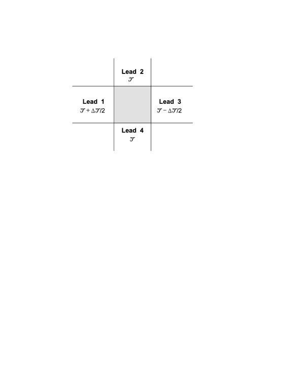
Figure 1: Schematic diagram of the four-terminal cross-bar sample. The area with SOI is marked by gray. A thermal gradient $\Delta\mathcal{T}$ is applied between the longitudinal lead-$1$ and lead-$3$.

In the tight-binding representation, the Hamiltonian with SOI can be written as:ref15 ,

$$H = \sum_{\mathbf{i}\sigma}\varepsilon_{\mathbf{i}}c_{\mathbf{i}\sigma}^{{\dagger}}c_{\mathbf{i}\sigma}+\sum_{\mathbf{i}\sigma\sigma^{\prime}}[c_{\mathbf{i}+\delta y,\sigma}^{{\dagger}}(-t\mathbf{I}-i\sigma_{x}V_{R})_{\sigma\sigma^{\prime}}c_{\mathbf{i}\sigma^{\prime}}$$ (1)

$$+c_{\mathbf{i}+\delta x,\sigma}^{{\dagger}}(-t\mathbf{I}+i\sigma_{y}V_{R})_{\sigma\sigma^{\prime}}c_{\mathbf{i}\sigma^{\prime}}+H.c.]$$

where $c_{\mathbf{i}\sigma}^{{\dagger}}$($c_{\mathbf{i}\sigma}$) is the creation (annihilation) operator of electrons in the site $\mathbf{i}=(n,m)$ with spin $\sigma$, and $\delta x$ and $\delta y$ are the unit vectors along the x and y directions. $\varepsilon_{\mathbf{i}}$ is the on-site energy, which is set to $0$ everywhere for the clean system. When the center region is a disorder system, $\varepsilon_{\mathbf{i}}$ is set by a uniform random distribution [-W/2,W/2]. Here $t=\hbar^{2}/(2m^{\ast}a^{2})$ is the hopping matrix element with the lattice constant $a$, $\mathbf{I}$ is a two-dimensional identity matrix. The strength of Rashba SOI is represents by $V_{R}=\alpha\hbar/2a$, where $\alpha$ is the Rashba spin-orbital coupling. $V_{R}$ is set to zero in the lead-2 and lead-4.

Considering a small temperature gradient $\Delta\mathcal{T}$ on the longitudinal lead-1,3, we can set the temperatures $\mathcal{T}_{1}=\mathcal{T}+\Delta\mathcal{T}/2$, $\mathcal{T}_{3}=\mathcal{T}-\Delta\mathcal{T}/2$, $\mathcal{T}_{2}=\mathcal{T}_{4}=\mathcal{T}$. The charge current in lead-$p$ can be written as $J_{pe}=e(I_{p\uparrow}+I_{p\downarrow})$ and the spin current is $J_{ps}=(\hbar/2)(I_{p\uparrow}-I_{p\downarrow})$. Here $I_{p\sigma}$ is the particle current in lead-$p$ with $\sigma$ equals to $\uparrow$ or $\downarrow$. $I_{p\sigma}$ can be obtained by the LB formula:ref0 ; ref15

$$I_{p\sigma}=\frac{1}{\hbar}\sum_{q\neq p}\int dE~{}T_{p\sigma,q}(E)[f_{p}(E)-f_{q}(E)]$$ (2)

where $T_{p\sigma,q}(E)$ is the transmission coefficient from the lead-$q$ to the lead-$p$ with spin $\sigma$ and $E$ is the energy of the incident electron. $f_{p}(E)$ is the electronic Fermi distribution function of the lead-$p$.

The spin Hall current in lead-2 and lead-4 can be calculated with the closed boundary condition in both lead-1,3 and lead-2,4, i.e. $V_{1}=V_{3}=0$ and $V_{2}=V_{4}=0$. From symmetry of the system, we know that $J_{2s}=-J_{4s}$ref0 . After the Taylor expansion, the spin Nernst coefficient $N_{s}\equiv J_{2s}/{\Delta\mathcal{T}}$ can be reduced to:

$$N_{s}=\frac{1}{4\pi}\int{dE}(\Delta T_{23}-\Delta T_{21})\frac{E-E_{F}}{k_{B}\mathcal{T}^{2}}f(1-f),$$ (3)

here $\Delta T_{2p}=T_{2\uparrow,p}-T_{2\downarrow,p}$, and $f$ is the zero order of Taylor expansion of the Fermi distribution function, it is the same for all four leads, $f(E)=1/\{\mathrm{exp}[(E-E_{F})/k_{B}\mathcal{T}]+1\}$.

Figure 2: $N_{s}$ (red solid) and $S$ (black dotted) vs. Fermi energy $E_{F}$ for different Rashba $V_{R}$. The (scaled) transmission coefficient $T_{1,2}+T_{1,3}$ (thin blue dashed) and spin transmission coefficient $\Delta T_{2,3}$ (thin blue solid) are also shown. The other parameters are $\mathcal{T}=0.01$, and $L=19a$.

For the calculation of the longitudinal seebeck coefficient $S$, we need the open boundary condition at lead-1,3, i.e. $J_{1e}=J_{3e}=0$ to find the difference $\Delta V=V_{1}-V_{3}$. Different from a quasi-one-dimensional 2-leads systemseebeck1 , the extra leads-2,4 also affects the longitudinal seebeck coefficient $S$ of the entire system. For example, with a perpendicular magnetic field $B$, the longitudinal seebeck coefficient $S$ is affected by the bias in leads-2,4, $V_{2}\$and $V_{4}$. However, without $B$, the sample’s symmetry increases from $C_{2}$ symmetry to $D_{2}$ symmetry, i.e., we have $T_{1,2}=T_{1,4}$, Here $T_{1,2}=T_{1\uparrow,2}+$ $T_{1\downarrow,2}$. After the Taylor expansion, we can get the longitudinal seebeck coefficient $S\equiv-\Delta V/\Delta\mathcal{T}$ as:

$$S=\frac{1}{\mathcal{T}}\frac{\int dE~{}\left(T_{1,2}+T_{1,4}+2T_{1,3}\right)(E-E_{F})f\left(1-f\right)}{\int dE\left(T_{1,2}+T_{1,4}+2T_{1,3}\right)f\left(1-f\right)}.$$ (4)

The equation above shows that, even with a higher symmetry, the longitudinal seebeck coefficient $S$ is still affected by the transport properties from lead-2 and lead-4.

With the $D_{2}$ symmetry, the relationship between $S$ and $N_{s}$ can be further derived. In fact, we can rewritten $S=\left(A^{\downarrow}+A^{\uparrow}\right)\left/\left[\int dEF\left(\varepsilon\right)\left(a^{\uparrow}+a^{\downarrow}\right)\right]\right.$. The $D_{2}$ symmetry gives $\Delta T_{23}=-\Delta T_{21}$. Noticing $T_{3\uparrow,1}=T_{3\downarrow,1}$, the spin Nernst coefficient can be simplified as $N_{s}\ =\left.\left(A^{\downarrow}-A^{\uparrow}\right)\right/\left(2\pi k_{B}\mathcal{T}\right)$. Here $\varepsilon=E-E_{F}$ and $F\left(\varepsilon\right)=f\left(1-f\right)$, $a^{\uparrow}$ denotes the spin up term: $a^{\uparrow}=T_{2\uparrow,1}+T_{3\uparrow,1}$, and $a^{\downarrow}$ the spin down term $a^{\downarrow}=T_{2\downarrow,1}+T_{3\downarrow,1}$, we also use the notation of the integral term $A^{\uparrow}=\left.\int dE\varepsilon F\left(\varepsilon\right)a^{\uparrow}\right/\mathcal{T}$ and $A^{\downarrow}=\left.\int dE\varepsilon F\left(\varepsilon\right)a^{\downarrow}\right/\mathcal{T}$. Because of the symmetry, only leads-1,2,3 are used in the simplified expression of $S$ and $N_{s}$, we only need the upper half of the sample for our investigation. In fact, $\ a^{\uparrow}$ ($a^{\downarrow}$) and $A^{\uparrow}$ ($A^{\downarrow}$) reflects transport properties of spin-up (spin-down) electrons in the upper half of the sample. Roughly speaking, $S$ can be seen as the sum of spin-up and spin-down terms, while $N_{s}\$ as the difference of them.

In the numerical calculations, $t=\hbar^{2}/(2m^{\ast}a^{2})$ is set as the energy unit. If taking the effective electron mass $m^{\ast}=0.05m_{e}$ and the lattice constant $a=12.5nm$, $t$ is about $5meV$. Temperature is fixed by $k_{B}\mathcal{T}=0.01t$, which is about $1K$. The size of center region is $L=19a$, about $237nm$. In a reasonable experimental range thus far $V_{R}\in\left[0,0.1\right]$soi . However, in order to thoroughly study the relationship between the spin Nernst coefficient $N_{s}$ and the seebeck coefficient $S$, we extend the range of $V_{R}\$up to $\left[0,1\right]$ in our calculation.

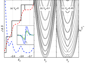
Figure 3: (a) A simple model: Current $J$ because of voltage gradient(red dashed) and thermal power $S$ because of thermal gradient (blue dotted) vs. Fermi energy $E_{F}$ at a two-lead system with Rashba $V_{R}=0$. The (scaled) transmission function $T_{1,3}$ is also shown (black solid). The plot in the small box shows $f_{L}-f_{R}$ with temperature difference. (b) and (c): the eigen energy of the lead $E_{n,k_{y}}$ v.s. longitudinal wave vector $k_{y}$ (units: $1/2a$) for different $V_{R}$

Fig.2 shows the spin Nernst coefficient $N_{s}$ and the seebeck coefficient $S$ versus the Fermi Energy $E_{F}$ in the clean system ($W=0$). It is clearly seen that the seebeck coefficient $S$ peaks at the positions where there are step-changes of transmission function $T_{1,2}+T_{1,4}$. These peaks can be explained by a simple model only with a 2-lead system without the Rashba SOI, shown in Fig.3(a). The transmission coefficient $T_{1,3}$ is a step function (solid-black curve). The reason is as follows. The sample can be considered as a multi-channel system at a low temperature (here $T\sim 1K$). When fermi energy increases, more channels in the lead are used to transport current. Thus, $\Delta V$ of two leads as well as the current increase with increasing of fermi energy (red-dashed curve). However, the $S$ (blue-dotted curve) can not accumulates while $E_{F}$ increases, it only peaks while the channel number changes and $S$ is close to zero with a fixed channel number. This can be seen from the LB formula (2), if lead-p and lead-q have different temperatures, $f_{p}(E,T+\Delta T)-f_{q}(E,T-\Delta T)$ is an antisymmetry function of $E-E_{F}$ (see plot in small box of Fig.3(a)): when $E<E_{F}$, $f_{p}<f_{q}$, current flows from lower temperature lead to higher temperature one; when $E>E_{F}$, current flows in the opposite direction. Only when the two flows are not equal, i.e. $T_{p\sigma,q}$ has an antisymmetry part, we can have a nonzero current. Thus for Fig.3(a), only when $T_{1,3}$ is at the step-change point, it has antisymmetry part and can give a non-zero $S$.

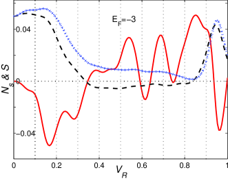
Figure 4: ($N_{s}$ (red solid) and $S$ (black dashed) vs. Rashba SOI $V_{R}$ for fermi energy $E_{F}=-3$. For compare, the blue dotted line shows the seebeck when lead-2,4 have the same $V_{R}$ as lead-1,3. The other parameters are $\mathcal{T}=0.01$, and $L=19a$.

This conclusion can also be used to analyst spin-involved quantities. From Fig.2, we can see that $N_{s}$ (red solid line) shows an oscillatory structure. Besides the peaks at $V_{R}=0$ ($N_{s}$ is zero at this point), the magnitude of $N_{s}$ oscillation is also large at the peaks of $S$; but at the exact maximum point of $S$, where $V_{R}$ is quite small ($V_{R}\lesssim 0.1$), $N_{s}$ is generally close to zero. This is because the spin transmission coefficient $\Delta T_{2,3}$ generally has an extreme value when the transmission coefficient jumps at a step. Around an extreme value, any function is almost symmetry, thus one only can get a low value of $N_{s}$. While at both sides of the extreme value, $\Delta T_{2,3}$ monotonically increases or decreases, we can get a local maximum magnitude of $N_{s}$. Now why $\Delta T_{2,3}$ has an extreme value at a peak of $S$ for a small $V_{R}$. Due to the Rashba SOI, each eigen-energy band splits into two sub-bands with opposite spin directions. These two sub-bands degenerate at $k_{y}=0$, and the lower sub-band has two valleys below this degenerate point. The two sub-bands are very close to each other when $V_{R}$ is small. If the lower sub-band of high level (for example, $E_{1,k_{y}}$) has the similar spin direction with the upper sub-band of low level energy (for example, $E_{0,k_{y}}$), $\Delta T_{2,3}$ continually increases when $E_{F}$ goes from the upper band of $E_{0,k_{y}}$ to the two valleys of lower sub-band of $E_{1,k_{y}}$, and than rapidly decreases when $E_{F}$ goes through the degenerate point ($k_{y}=0$) of $E_{1,k_{y}}$, thus we get a peak in $\Delta T_{2,3}$; otherwise we get a valley in $\Delta T_{2,3}$.

When $V_{R}$ is very big, we can see the external peaks for both $N_{s}$ and $S$. For example $V_{R}=0.45$ in Fig.2(d), close to the $2^{nd}$ and $3^{rd}$ main peaks of $S$, we can see a very sharp sub-peak of $N_{s}$. In fact, these are also the small peaks of $S$, though not very big. This is because for these two band (see Fig.3(c)), the two valleys of the lower sub-band is far from the degenerate point at $k_{y}=0$, the two channel of these two sub-bands is separated. Thus we can see two peaks. At this time, the change of spin transmission coefficients can be roughly thought as the change of transmission coefficients, thus we can see $N_{s}$ peaks at the $S$’s peak.

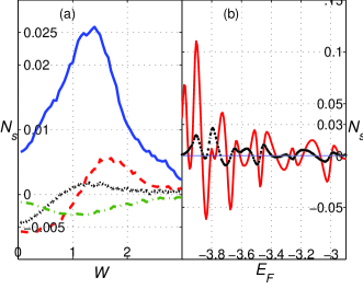
Figure 5: (a). $N_{s}$ vs. the strength of disorder $W$ for different Fermi level $E_{F}=-3.8$(solid blue), $E_{F}=-3.6$(dashed red), $E_{F}=-3.0$(dotted black), $E_{F}=-2.2$(dotted dashed green); (b). $N_{s}$ vs. Fermi energy $E_{F}=-3.8$ for $W=0$ (dashed black) and $W=1.4$ (solid black).Other parameters are $V_{R}=0.05$, $\mathcal{T}=0.01$, and $L=19a$.

In Fig.4, we show the spin Nernst coefficient $N_{s}$ and the seebeck coefficient $S$ versus the Rashba SOI $V_{R}$ in the clean system ($W=0$) for $E_{F}=-3$. The seebeck coefficient $S$ decreases and maintains for a small value for quite a while before shows another peak. This is because increasing $V_{R}$ moves the energy bands and makes them go through the fermi energy. It should be mentioned that we found the negative seebeck coefficient $S$ (Fig. 2d), which means a longitudinal current occurs in the opposite direction of the temperature gradient $\Delta\mathcal{T}$. This is due to the boundary conditions $V_{R}=0$ at leads-2,4. As a compare, we also show $S$ for a uniform system, i.e. leads-2,4 having the same strength of $V_{R}$ as in the sample. For this situation, the seebeck coefficient $S$ is no longer negative. In fact, when the Rashba SOI is absent in the leads-2,4, an interface between $V_{R}=0$ and $V_{R}\neq 0$ ocurrsref0 , this interface causes additional scattering for an incident electron. In some special case like $E_{F}=-3$, this may make the electrons below $E_{F}$ easier to transport than the electrons above $E_{F}$, thus a negative $S$.

Finally we discuss the disorder effect on the spin Nernst effect. Fig.5 shows $N_{s}$ versus disorder strength $W$ for different Fermi energies. The calculations are averaged over $500$ disorder configurations. Around $W<1.7$, $N_{s}$ shows an oscillatory structure. $N_{s}$ changes sign with increasing of the disorder strength (see $E_{F}=-3.6$ and $-3.0$ in Fig.5). It is interesting to see that, comparing to a clean system ($W=0$), $N_{s}$ can be unexpectedly increased by disorder $W$. This is because the disorder changes the oscillating structure of $N_{s}$ (see Fig.5b). As expected, the disorder decreases the strength of oscillating, however, it also shifts the peak positions of $N_{s}$. It is possible to have a peak in $N_{s}$ at finite disorder while it is almost zero initially at clean limit. In Fig.5a, around $W=1\sim 1.5$, for the Fermi level $E_{F}=-3.8$, $-2.2$, we can see that $N_{s}$ is up to about three times of $N_{s}$ at $W=0$. The behavior of $N_{s}$ v.s. $W$ is very apparent when the Fermi level $E_{F}$ is close to the bottom of energy band ($E_{F}=-4$). For $E_{F}=-3.8$, $N_{s}$ is much bigger than those at other Fermi levels, and we can see a very remarkable peak at about $W=1.4$. For $E_{F}=-2.2$, $N_{s}$ begins from $-0.005$, changes its sign at about $W\sim 1.25$ and than increases, again reaches to $0.005$ at about $W\sim 1.75$. With a very big disorder, $N_{s}$ should go to zero as system enters into an insulating regime. We find that the zero of $N_{s}$ occurs at $W=3$ for $V_{R}=0.05.$ This is roughly independent of the locations of the Fermi energy.

In summary, in the absence of a perpendicular magnetic field, the interplay between the spin Nernst effect and the seebeck effect is investigated in a two-dimensional cross-bar with a spin-orbit interaction. The spin Nernst effect exhibits an oscillatory structure for a wide range of the Rashba SOI. With a large Rashba SOI, the $N_{s}$ oscillation has a peak when the seebeck coefficient possesses one. However, the inverse condition is not always satisfied, namely, the seebeck coefficient can be almost zero while $N_{s}$ has a peak. The disorder effect on the spin Nernst effects is also studied. We find that disorder can enhance $N_{s}$ up to three times for some Fermi levels. In addition, the disorder can also change the sign of spin Nernst effect. Moreover, the limit of disorder where $N_{s}$ goes to zero is independent of the Fermi energy.

Acknowledgments: We thank Q.F. Sun and S.G. Cheng for many helpful discussions. We gratefully acknowledge the financial support from US-DOE under DE-FG02-04ER46124 and US-NSF.

References

- (1) Electronic address: xuele@okstate.edu
- (2) A.S. Dzurak, et al., Phys. Rev. B 55, R10197 (1997); R. Scheibner, et al., Phys. Rev. Lett. 95, 176602 (2005); Phys. Rev. B 75, 041301 (2007).
- (3) L.W. Molenkamp, et al., Phys. Rev. Lett. 65, 1052 (1990).
- (4) A.A. Abrikosov, Fundamentals of the theory of metals (NorthHolland Amsterdam, 1988).
- (5) J.M. Iiman, Electrons and phonons (Oxford university Press, Oxford, U.K., 1960).
- (6) C.W.J. Beenakker and A.A.M. Staring, Phys. Rev. B 46, 9667 (1992).
- (7) H. Nakamura, N. Hatano, R. Shirasaki, Solid State Communications 135 (2005); R. Shirasaki, H. Nakamura, N. Hatano, J. Surf. Sci. Nanotech. Vol. 3, 518 (2005).
- (8) K. Behnia, et al., Phys. Rev. Lett. 98, 166602 (2007); Science 317, 1729 (2007).
- (9) Shu-guang Cheng, Yanxia Xing, Qing-feng Sun, and X. C. Xie, Phys. Rev. B 78, 045302 (2008).
- (10) L. Sheng, D. N. Sheng, and C. S. Ting, Phys. Rev. Lett. 94, 016602 (2005); W. Ren, et al., Phys. Rev. Lett. 97, 066603 (2006); Z. Qiao, J. Wang, and H. Guo, Phys. Rev. Lett. 98, 196402 (2007); Y. Xing, Q.-F. Sun, and J. Wang, Phys. Rev. B 75, 075324 (2007).
- (11) M. Cutler and N. F. Mott, Phys. Rev. Lett. 88, 136601 (2002).
- (12) T. P. Pareek, cond-mat/0412115v2; Takaaki Koga, et al., Phys. Rev. Lett. 89, 046801 (2002); G. Engels, et al., Phys. Rev. B 55, R1958 (1997).
- (13) H. Jiang, L. Wang, Q.F. Sun, and X.C. Xie, to appear in Phys. Rev. B (arXiv:0905.4550).